New statistical methodology for second level global sensitivity analysis

Abstract

Global sensitivity analysis (GSA) of numerical simulators aims at studying the global impact of the input uncertainties on the output. To perform the GSA, statistical tools based on inputs/output dependence measures are commonly used. We focus here on dependence measures based on reproducing kernel Hilbert spaces: the Hilbert-Schmidt Independence Criterion denoted HSIC. Sometimes, the probability distributions modeling the uncertainty of inputs may be themselves uncertain and it is important to quantify the global impact of this uncertainty on GSA results. We call it here the second-level global sensitivity analysis (GSA2). However, GSA2, when performed with a double Monte Carlo loop, requires a large number of model evaluations which is intractable with CPU time expensive simulators. To cope with this limitation, we propose a new statistical methodology based on a single Monte Carlo loop with a limited calculation budget. Firstly, we build a unique sample of inputs from a well chosen probability distribution and the associated code outputs are computed. From this inputs/output sample, we perform GSA for various assumed probability distributions of inputs by using weighted HSIC measures estimators. Statistical properties of these weighted estimators are demonstrated. Finally, we define 2${}^{\text{nd}}$-level HSIC-based measures between the probability distributions of inputs and GSA results, which constitute GSA2 indices. The efficiency of our GSA2 methodology is illustrated on an analytical example, thereby comparing several technical options. Finally, an application to a test case simulating a severe accidental scenario on nuclear reactor is provided.

1 Introduction

Numerical simulators (or computer codes) are fundamental tools for understanding, modeling and predicting phenomena. They are widely used nowadays in several fields such as physics, chemistry and biology, but also in economics and social science. These numerical simulators take a large number of input parameters more or less uncertain, characterizing the studied phenomenon. Consequently, the output which is provided by the numerical code is also uncertain. It is therefore important to consider not only the nominal values of inputs, but also the set of all possible values in the range of variation of each uncertain parameter [13, 24]. In the framework of a probabilistic approach, the inputs and the output are considered as random variables and their uncertainties are modeled by probability distributions. The objective is then to evaluate the impact of the input uncertainties on the variability of the output. For this, sensitivity analysis studies can be performed, using statistical methods based on code simulations (also called realizations or observations). To choose these numerical simulations, experimental design techniques can be used (see e.g. [11]).

Generalities on sensitivity analysis. Sensitivity analysis [35] aims at determining how the variability of inputs contributes, qualitatively or quantitatively, to the output variability. Sensitivity analysis can yield a screening of the inputs, which consists in separating the inputs into two subgroups: those that significantly influence the output value (significant inputs) and those whose influence on the output can be neglected. More generally, sensitivity analysis can be divided into two main areas:

• local sensitivity analysis (LSA) which studies the output variability for a small input variation around nominal values (reference values);

• global sensitivity analysis (GSA) which studies the impact of the input uncertainties on the output, considering the whole range of input variation.

We focus here on GSA and we call it in the following, first-level GSA, denoted GSA1.

Use of dependence measures for GSA1. Among GSA1 tools [25], one of the most popular methods used in industrial applications is based on a variance decomposition of the output [38]. The sensitivity indices thus obtained by this decomposition are called Sobol’ indices. These indices have the advantage of being easily interpretable but are in practice very expensive in computing time (several tens of thousands of code simulations required). More recently, tools based on dependence measures have been proposed for GSA1 purpose [10]. These measures aim at quantifying, from a probabilistic point of view, the dependence between the output random variable and the input random variables. Among these measures, we can mention the $f$-divergence of Csiszár which, for a given input, compares the distribution of the output and its distribution when this input is fixed, thanks to a function with specific properties (see [9] for more details). Always on the same principle, the distance correlation is an other dependence measure which compares the characteristic function of a couple of random input/output variables, with the product of the joint characteristic functions of the two variables [42]. Last but not least, the Hilbert-Schmidt independence criterion denoted HSIC [22], generalizes the notion of covariance between two random variables and takes into account a very large spectrum of forms of dependence between variables. Initially developed by statisticians [22] to perform independence tests, these dependence measures offer the advantage of having a low cost of estimation (in practice a few hundred simulations against several tens of thousands for Sobol’ indices) and their estimation for all inputs does not depend on the number of inputs. In addition, recent work proposed by [12] showed the efficiency of these measures to perform a screening of the input variables, from various HSIC-based statistical tests of significance. Finally, HSIC measures can easily be extended to non-vector inputs (functional, categorical, etc.). For all these reasons, we will focus here on HSIC measures for GSA1 of numerical simulators.

Second-level input uncertainties and GSA2. In some cases, the probability distributions characterizing the uncertain inputs may themselves be uncertain. This uncertainty may be related to a divergence of expert opinion on the probability distribution assigned to each input or a lack of information to characterize this distribution. The modeling of this lack of knowledge on input laws can take many forms:

• the type of the input distribution is uncertain (uniform, triangular, normal law, …);

• the distribution is known but its parameters are uncertain (e.g., known normal distribution with unknown mean and variance, eventually estimated on data).

In both cases, the resulting uncertainties on the input laws are referred to here as second-level uncertainties. As part of a probabilistic approach, these uncertainties can be modeled by a probability law on a set of possible probability laws of inputs or by a probability law on the parameters of a given input law (e.g. Gaussian distribution with probability law on mean and/or variance). In any case, these 2${}^{\text{nd}}$-level uncertainties can significantly change the GSA1 results performed by HSIC or any other dependence measure. In this framework, the main purpose of second-level GSA denoted GSA2 is to answer the following questions: «What impact do 2${}^{\text{nd}}$-level uncertainties have on the GSA1 results?» and «What are the most influential ones and those whose influence is negligible?». The GSA2 results and conclusion can then be used to prioritize the characterization efforts on the inputs whose uncertainties on probability laws have the greatest impact on GSA1 results. Note that, we assume here that the inputs are independent and continuous random variables with a probability density function, denoted here pdf.

Practical problems raised by GSA2. In practice, the realization of GSA2 raises several issues and technical locks. First, it is necessary to characterize GSA1 results, i.e. to define a representative quantity of interest in order to compare the results obtained for different uncertain input pdf. Then, the impact of each uncertain input pdf on this quantity of interest has to be evaluated. For this, sensitivity indices measuring the dependence between GSA1 results and each input pdf have to be defined. We propose to call them 2${}^{\text{nd}}$-level GSA indices. In order to estimate these measures, an approach based on a "double Monte Carlo loop" could be considered. In the outer loop, a Monte Carlo sample of input pdfs is sorted, while the inner loop aims at evaluating the GSA1 results associated to each pdf. For each pdf selected in the outer loop, the inner loop consists in generating a Monte Carlo sample of code simulations (set of inputs/output) and to compute GSA1 results. The process is repeated for each input pdf. At the end of the outer loop, the impact of input pdf on the GSA1 results can be observed and quantify by computing 2${}^{\text{nd}}$-level GSA. Unfortunately, this type of double loop approach requires in practice a very large number of simulations which is intractable for time expensive computer codes. Therefore, other less expensive approaches must be developed.
To answer these different issues (choice of the quantity of interest, definition of 2${}^{\text{nd}}$-level sensitivity indices and reduction of the budget of simulations), we propose in this paper a "single loop" Monte Carlo methodology for GSA2 based on both 1${}^{\text{st}}$-level and 2${}^{\text{nd}}$-level HSIC dependence measures.

The paper is organized as follows. In Section 2, we introduce HSIC measures, before presenting the statistical estimators of these measures, as well as the associated characteristics (bias, variance, asymptotic law). Then, we show that these measures can be formulated and estimated with a sample generated from a different distribution than the prior distribution of the inputs. For this, new estimators are proposed and their characteristics are detailed, these new estimators being a key point for the proposed GSA2 methodology. In Section 3, the full methodology for GSA2 is presented: a single inputs/output sample is used, taking advantage of the new HSIC estimators. The GSA2 principle and the related practical issues are first introduced. The general algorithm is then detailed, followed by dedicated sections focusing on major technical elements. In Section 4, the methodology is illustred on an analytical example, thereby comparing different options and technical choices of the methodology. Finally, an application on a test case simulating a severe accidental scenario on a nuclear reactor is proposed.

2 Statistical inference around Hilbert-Schmidt dependence measures (HSIC)

Throughout the rest of this document, the numerical model is represented by the relation:

$$Y=F\left(X_{1},\ldots,X_{d}\right),$$

where $X_{1},\ldots,X_{d}$ and $Y$ are respectively the $d$ uncertain inputs and the uncertain output, evolving in one-dimensional real areas respectively denoted $\mathcal{X}_{1},\ldots,\mathcal{X}_{d}$ and $\mathcal{Y}$. $F$ denotes the numerical simulator. We note $\mathbf{X}=\left(X_{1},\ldots,X_{d}\right)$ the vector of inputs. As part of the probabilistic approach, the $d$ inputs are considered as continuous and independent random variables with known densities. These densities are respectively denoted $f_{1},\ldots,f_{d}$. Finally, $f(x_{1},\ldots,x_{d})=f_{1}(x_{1})\times\ldots\times f_{d}(x_{d})$ denotes the density of the random vector $\mathbf{X}$. As the model $F$ is not known analytically, a direct computation of the output probability density as well as dependence measures between $\mathbf{X}$ and $Y$ is impossible. Only observations (or realisations) of $F$ are available. It is therefore assumed in the following that we have a $n$-sample of inputs and associated outputs $\left(\mathbf{X}^{(i)},Y^{(i)}\right)_{1\leq i\leq n}$, where $Y^{(i)}=F(\mathbf{X}^{(i)})$ for $i=1,\ldots,n$.

2.1 Review on HSIC measures

After introducing their theoretical definition, the estimation of HSIC dependence measures and their use for GSA1 are detailed.

2.1.1 Definition and description

To define the HSIC measure between $X_{k}$ and $Y$ (where $k\in\{1,\ldots,d\}$), [22] associate to $X_{k}$ a reproducing kernel Hilbert space (denoted RKHS, see [3] for more details) $\mathcal{F}_{k}$ composed of functions mapping from $\mathcal{X}_{k}$ to $\mathbb{R}$ and characterized by a kernel $l_{k}$. The same transformation is carried out for $Y,$ considering a RKHS denoted $\mathcal{G}$ and a kernel $l$. The scalar products on $\mathcal{F}_{k}$ and $\mathcal{G}$ are respectively denoted $\langle.,.\rangle_{\mathcal{F}_{k}}$ and $\langle.,.\rangle_{\mathcal{G}}$. Under this RKHS framework, [4] defines the cross-covariance operator $C_{k}$ between $\mathcal{F}_{k}$ and $\mathcal{G}$ as the linear operator from $\mathcal{G}$ to $\mathcal{F}_{k}$ defined for all $f\in\mathcal{F}_{k}$ and all $g\in\mathcal{G}$ by:

$$\langle f,C_{k}g\rangle_{\mathcal{F}_{k}}=\operatorname{Cov}(f(X_{k}),g(Y)).$$

The operator $C_{k}$ generalizes the notion of covariance, taking into account a large spectrum of relationships between $X_{k}$ and $Y$ (not only linear).

Finally, the Hilbert-Schmidt independence criterion (HSIC) is defined by [22] as the Hilbert-Schmidt norm of the operator $C_{k}$:

$$\operatorname{HSIC}(X_{k},Y)_{\mathcal{F}_{k},\mathcal{G}}=\|C_{k}\|_{\operatorname{HS}}^{2}=\displaystyle\sum_{i,j}\,\langle u_{i},C_{k}(v_{j})\rangle_{\mathcal{F}_{k}}^{2},$$ (1)

where $\left(u_{i}\right)_{i\geq 0}$ and $\left(v_{j}\right)_{j\geq 0}$ are respectively orthonormal bases of $\mathcal{F}_{k}$ and $\mathcal{G}$.

Remark 2.1.

In the following, the notation $\operatorname{HSIC}(X_{k},Y)_{\mathcal{F}_{k},\mathcal{G}}$ is replaced by $\operatorname{HSIC}(X_{k},Y)$ in order to lighten the expressions.

Authors of [22] show that the HSIC measure between an input $X_{k}$ and the output $Y$ can be expressed using the kernels $l_{k}$ and $l$ in a more convenient form:

$$\operatorname{HSIC}(X_{k},Y) =\mathbb{E}\left[l_{k}(X_{k},X^{\prime}_{k})l(Y,Y^{\prime})\right]+\mathbb{E}\left[l_{k}\left(X_{k},X^{\prime}_{k}\right)\right]\mathbb{E}\left[l\left(Y,Y^{\prime}\right)\right]$$ (2)

$$-2\mathbb{E}\left[\mathbb{E}\left[l_{k}\left(X_{k},X^{\prime}_{k}\right)\mid X_{k}\right]\mathbb{E}\left[l\left(Y,Y^{\prime}\right)\mid Y\right]\right],$$

where $(X^{\prime}_{1},\ldots,X^{\prime}_{d})$ is an independent and identically distributed copy of $(X_{1},\ldots,X_{d})$ and $Y^{\prime}=F\left(X^{\prime}_{1},\ldots,X^{\prime}_{d}\right)$.

Independence characterization. The nullity of $\operatorname{HSIC}(X_{k},Y)$ is not always equivalent to the independence between $X_{k}$ and $Y$: this characteristic depends on the RKHS associated to $X_{k}$ and $Y$. To ensure equivalence between $\operatorname{HSIC}$ nullity and independence, the kernels $l_{k}$ and $l$ must belong to the specific class of universal kernels [32]. A kernel is said to be universal if the associated RKHS is dense in the space of continuous functions w.r.t the infinity norm. However, the universality is a very strong assumption, especially on non-compact spaces. Let us mention as example the Gaussian kernel (the most commonly used for real variables) which is universal only on compact subsets $\mathcal{Z}$ of $\mathbb{R}^{q}$ [40]. This kernel is defined for a pair of variables $(z,z^{\prime})\in\mathbb{R}^{q}\times\mathbb{R}^{q}$ by:

$$k_{\lambda}(z,z^{\prime})=exp\left(-\lambda\|z-z^{\prime}\|_{2}^{2}\right),$$ (3)

where $\lambda$ is a positive real parameter (fixed) and $\|.\|_{2}$ is the euclidean norm in $\mathbb{R}^{q}$.

First referred to as probability-determining kernels [18], the notion of characteristic kernels [19], which is a weaker assumption than universality, has been lately introduced. It has been proven that this last assumption is sufficient for independence characterization using HSIC. In fact, when the kernels $l$ and $l_{k}$ are characteristic then, $\operatorname{HSIC}(X_{k},Y)=0$ iff $X_{k}$ and $Y$ are independent (see e.g. [41]). In particular, the Gaussian kernel defined in Formula (3) is characteristic on the entire $\mathbb{R}^{q}$ [19].

Remark 2.2.

There is no theoretical result for the optimal choice for the kernel width $\lambda$ in (3). In practice, two main options are adopted for the adjustment of $\lambda$: whether the inverse of empirical variance of $z$, or the inverse of empirical median of $\|z-z^{\prime}\|_{2}^{2}$. In the following, for the computation of $\operatorname{HSIC}(X_{k},Y)$, we choose the first option for both kernels associated to $X_{k}$ and $Y$. We propose to call the $\operatorname{HSIC}$ measures built with these kernels: $\operatorname{HSIC}$ measures with standardized Gaussian kernel.

2.1.2 Statistical estimation

In this paragraph, we present HSIC estimators, as well as their characteristics. As a reminder, we assume that we have a n-sample of independent realizations $\left(\mathbf{X}^{(i)},Y^{(i)}\right)_{1\leq i\leq n}$ of the inputs/output couple $(\mathbf{X},Y)$ where $\mathbf{X}=(X_{1},\ldots,X_{d})$.

Monte Carlo estimation. From Formula (2), authors of [22] propose to estimate each $\operatorname{HSIC}(X_{k},Y)$ by:

$$\widehat{\operatorname{HSIC}}(X_{k},Y)=\displaystyle\frac{1}{n^{2}}\displaystyle\sum_{1\leq i,j\leq n}(L_{k})_{i,j}L_{i,j}+\displaystyle\frac{1}{n^{4}}\displaystyle\sum_{1\leq i,j,q,r\leq n}(L_{k})_{i,j}L_{q,r}-\displaystyle\frac{2}{n^{3}}\displaystyle\sum_{1\leq i,j,r\leq n}(L_{k})_{i,j}L_{j,r},$$ (4)

where $L_{k}$ and $L$ are the matrices defined for all $(i,j)\in\{1,\ldots,n\}$ by $(L_{k})_{i,j}=l_{k}(X_{k}^{(i)},X_{k}^{(j)})$ and $(L)_{i,j}=l\left(Y^{(i)},Y^{(j)}\right)$.

These V-statistic estimators can also be written in the following more compact form (see [22]):

$$\widehat{\operatorname{HSIC}}(X_{k},Y)=\displaystyle\frac{1}{n^{2}}Tr(L_{k}HLH),$$ (5)

where $H$ is the matrix defined by $H=\left(\delta_{i,j}-\displaystyle\frac{1}{n}\right)_{1\leq i,j\leq n}$, with $\delta_{i,j}$ the Kronecker symbol between $i$ and $j$ which is equal to $1$ if $i=j$ and $0$ otherwise.

Remark 2.3.

The estimator of Equation (4) is part of a class of estimators called V-statistics (in the name of Richard Von Mises [33]), which, althought being biased (but asymptotically unbiased), are more easily computable than an unbiased version based on U-statistics.

Characteristics of HSIC estimators. Under the assumption of independence between $X_{k}$ and $Y$ and the assumption $l_{k}(x_{k},x_{k})=l(y,y)=1$ (as in the case of Gaussian kernels), the estimator $\widehat{\operatorname{HSIC}}(X_{k},Y)$ is asymptotically unbiased, its bias converges in $O(\frac{1}{n})$, while its variance converges to $0$ in $O(\frac{1}{n^{2}})$. Moreover, the asymptotic distribution of $n\times\widehat{\operatorname{HSIC}}(X_{k},Y)$ is an infinite sum of independent $\chi^{2}$ random variables, which can be approximated by a Gamma law [36] with shape and scale parameters, respectively denoted $\gamma_{k}$ and $\beta_{k}$:

$$\gamma_{k}\simeq\displaystyle\frac{e^{2}_{k}}{v_{k}}\;,\;\beta_{k}\simeq\displaystyle\frac{n.v_{k}}{e_{k}}$$

where $e_{k}$ and $v_{k}$ respectively are the expectation and the variance of $\widehat{\operatorname{HSIC}}(X_{k},Y)$, i.e. $e_{k}=\mathbb{E}\left[\widehat{\operatorname{HSIC}}(X_{k},Y)\right]$ and $v_{k}=\mathrm{\operatorname{Var}}\left(\widehat{\operatorname{HSIC}}(X_{k},Y)\right)$. The reader can refer to [23] and [12] for more details on $e_{k}$ and $v_{k}$ and their estimation.

2.1.3 Use for first-level GSA

Several methods based on the use of HSIC measures have been developed for GSA1. In this paragraph, we mention three possible approaches: sensitivity indices [10], asymptotic tests [23] and permutation (also referred to as bootstrap) tests [12].

HSIC-based sensitivity indices. These indices directly derived from HSIC measures, classify the input variables $X_{1},..,X_{d}$ by order of influence on the output $Y$. They are defined for all $k\in\{1,\ldots,d\}$ by:

$$\operatorname{R}2^{2}_{\operatorname{HSIC},k}=\displaystyle\frac{\operatorname{HSIC}(X_{k},Y)}{\sqrt{\operatorname{HSIC}(X_{k},X_{k})\operatorname{HSIC}(Y,Y)}}.$$ (6)

The normalization in (6) implies that $\operatorname{R}2^{2}_{\operatorname{HSIC},k}$ is bounded and included in the range $[0,1]$ which makes its interpretation easier. In practice, $\operatorname{R}2^{2}_{\operatorname{HSIC},k}$ can be estimated using a plug-in approach:

$$\widehat{\operatorname{R}2}^{2}_{\operatorname{HSIC},k}=\displaystyle\frac{\widehat{\operatorname{HSIC}}(X_{k},Y)}{\sqrt{\widehat{\operatorname{HSIC}}(X_{k},X_{k})\widehat{\operatorname{HSIC}}(Y,Y)}}.$$ (7)

Asymptotic tests. The independence test between the input $X_{k}$ and the output $Y$ based on HSIC rejects the independence assumption between these two random variables (hypothesis denoted $\mathcal{H}_{0,k}$) when the p-value of the test based on the statistic $n\times\widehat{\operatorname{HSIC}}(X_{k},Y)$ is less than a threshold $\alpha$ (in practice $\alpha$ is set at $5\%$ or $10\%$). Within the asymptotic framework, this p-value denoted $\operatorname{P_{k}}$ is approximated under $\mathcal{H}_{0,k}$ using the Gamma approximation (denoted $\operatorname{G_{k}}$) of $n\times\widehat{\operatorname{HSIC}}(X_{k},Y)$ law:

$$\operatorname{P_{k}}\simeq 1-\operatorname{F}_{\operatorname{G_{k}}}\left(n\times\widehat{\operatorname{HSIC}}(X_{k},Y)_{obs}\right),$$ (8)

where $\operatorname{F}_{\operatorname{G_{k}}}$ is the cumulative distribution function of $\operatorname{G_{k}}$ and $\widehat{\operatorname{HSIC}}(X_{k},Y)_{obs}$ is the observed value of the random variable $\widehat{\operatorname{HSIC}}(X_{k},Y)$.

Permutation tests. Outside the asymptotic framework, independence tests based on permutation technique can be used. For this, the observed n-sample is resampled $B$ independent times considering random permutations denoted $\tau$ on the set $\{1,..,n\}$. For each bootstrap sample, the permutation is applied. This permutation is applied only to the vector $\mathbf{X}$ of inputs. We thus obtain $B$ bootstrap-samples $\left(\mathbf{X}^{\left(\tau^{[b]}(i)\right)},Y^{(i)}\right)_{1\leq i\leq n}$ with $1\leq b\leq B$. The HSIC measures computed on these samples are denoted $\left(\widehat{\operatorname{HSIC}}^{[b]}\right)_{1\leq b\leq B}$. The p-value (denoted $\operatorname{p_{k}}$) of the test is then computed by:

$$\operatorname{p_{k}}=\displaystyle\frac{1}{B}\sum_{b=1}^{B}\mathds{1}_{\widehat{\operatorname{HSIC}}^{[b]}(X_{k},Y)>\widehat{\operatorname{HSIC}}(X_{k},Y)}.$$ (9)

These different approaches can be used to screen the input variables by order of influence and consequently, to characterize, in the following, the GSA1 results.

2.2 Estimation of HSIC with a sample generated from an alternative distribution

In this part, we first demonstrate that HSIC measures presented in Section 2.1.1, can be expressed and then estimated using a sample generated from a probability distribution of inputs which is not their prior distribution. This sampling distribution will be called "alternative law" or "modified law". The characteristics of these new HSIC estimators (bias, variance, asymptotic law) will be presented. These estimators will then be used in the proposed methodology for 2${}^{\text{nd}}$-level global sensitivity analysis in Section 3.

2.2.1 Expression and estimation of HSIC measures under an alternative law

The purpose of this paragraph is to express HSIC measures between the inputs $X_{1},...,X_{d}$ and the output $Y$, using $d$ random variables $\widetilde{X}_{1}$, …, $\widetilde{X}_{d}$ whose laws are different from those of $X_{1}$, …, $X_{d}$. We assume that their densities denoted $\widetilde{f}_{1}$, $\widetilde{f}_{2}$, …, $\widetilde{f}_{d}$ have respectively the same supports as $f_{1}$, …, $f_{d}$. We denote in the following by $\mathbf{\widetilde{X}}$ and $\widetilde{Y}$ respectively the random vector $\mathbf{\widetilde{X}}=(\widetilde{X}_{1},...,\widetilde{X}_{d})$ and the associated output $\widetilde{Y}=F(\mathbf{\widetilde{X}})$. Finally, we designate by $\widetilde{f}(x_{1},..,x_{d})=\widetilde{f}_{1}(x_{1})\times\widetilde{f}_{2}(x_{2})\times...\times\widetilde{f}_{d}(x_{d})$ the density of $\mathbf{\widetilde{X}}$.

Changing the probability laws in HSIC expression is based on a technique commonly used in the context of importance sampling (see e.g. [5]). This technique consists in expressing an expectation $\mathbb{E}\left[g(Z)\right]$, where $Z$ is a random variable with density $f_{Z}$, by using a random variable $\widetilde{Z}$ with density $f_{\widetilde{Z}}$ whose support is the same as that of $f_{Z}$. This gives the following expression for $\mathbb{E}\left[g(Z)\right]$:

$$\mathbb{E}\left[g(Z)\right]=\displaystyle\int_{\operatorname{Supp(Z)}}g(z)\;f_{Z}(z)\;dz=\displaystyle\int_{\operatorname{Supp(Z)}}g(z)\;\displaystyle\frac{f_{Z}(z)}{f_{\widetilde{Z}}(z)}\;f_{\widetilde{Z}}(z)\;dz=\mathbb{E}_{\widetilde{f}}\left[g(\widetilde{Z})\;\displaystyle\frac{f_{Z}(\widetilde{Z})}{f_{\widetilde{Z}}(\widetilde{Z})}\right],$$ (10)

where the notation $\mathbb{E}_{\widetilde{f}}\left[h(Z)\right]$ designates the expectation of $h(Z)$ under the hypothesis $Z\sim\widetilde{f}$ and $\operatorname{Supp(Z)}$ denote the support of $Z$.

The HSIC measures, formulated as a sum of expectations in Equation (2), can then be expressed under the density $f_{\widetilde{Z}}$ by adapting Equation (10) to more general forms of expectations. Hence, we obtain:

$$\operatorname{HSIC}(X_{k},Y)=H^{1}_{k}+H^{2}_{k}H^{3}_{k}-2H^{4}_{k},$$ (11)

where $(H^{l}_{k})_{1\leq l\leq 4}$ are the real numbers defined by:

• $H^{1}_{k}=\mathbb{E}\left[l_{k}(\widetilde{X}_{k},\widetilde{X}^{\prime}_{k})l(\widetilde{Y},\widetilde{Y}^{\prime})\displaystyle w(\widetilde{X})w(\widetilde{X}^{\prime})\right]$;

• $H^{2}_{k}=\mathbb{E}\left[l_{k}\left(\widetilde{X}_{k},\widetilde{X}^{\prime}_{k}\right)w(\widetilde{X})w(\widetilde{X}^{\prime})\right]$;

• $H^{3}_{k}=\mathbb{E}\left[l\left(\widetilde{Y},\widetilde{Y}^{\prime}\right)w(\widetilde{X})w(\widetilde{X}^{\prime})\right]$;

• $H^{4}_{k}=\mathbb{E}\left[\mathbb{E}\left[l_{k}\left(\widetilde{X}_{k},\widetilde{X}^{\prime}_{k}\right)w(\widetilde{X}^{\prime})\mid\widetilde{X}_{k}\right]\mathbb{E}\left[l\left(\widetilde{Y},\widetilde{Y}^{\prime}\right)w(\widetilde{X}^{\prime})\mid\widetilde{Y}\right]\displaystyle w(\widetilde{X})\right]$

where $\mathbf{\widetilde{X}}^{\prime}$ is an independent and identically distributed copy of $\mathbf{\widetilde{X}}$, $\widetilde{Y}^{\prime}=F(\mathbf{\widetilde{X}}^{\prime})$ and $w=\displaystyle\frac{f}{\widetilde{f}}$.

Formula (11) shows that $\operatorname{HSIC}(X_{k},Y)$ with $k=1,...,d$ can then be estimated using a sample generated from $\widetilde{f}$, provided that $\widetilde{f}$ has the same support than the original density $f$. Thus, if we consider a $n$-sample of independent realizations $\left(\mathbf{\widetilde{X}}^{(i)},\widetilde{Y}^{(i)}\right)_{1\leq i\leq n}$, where $\mathbf{\widetilde{X}}$ is generated from $\widetilde{f}$ and $\widetilde{Y}^{(i)}=F(\widetilde{X}^{(i)})$ for $i=1,...,n$, we propose the following V-statistic estimator of $\operatorname{HSIC}(X_{k},Y)$:

$$\widetilde{\operatorname{HSIC}}(X_{k},Y)=\widetilde{H}^{1}_{k}+\widetilde{H}^{2}_{k}\widetilde{H}^{3}_{k}-2\widetilde{H}^{4}_{k},$$ (12)

where $(\widetilde{H}^{l}_{k})_{1\leq l\leq 4}$ are the V-statistics estimators of $(H^{l}_{k})_{1\leq l\leq 4}$.

Proposition 2.1.

Similarly to Equation (5), this estimator can be rewritten as:

$$\widetilde{\operatorname{HSIC}}(X_{k},Y)=\displaystyle\frac{1}{n^{2}}Tr\left(W\widetilde{L}_{k}WH_{1}\widetilde{L}H_{2}\right),$$ (13)

where $W$, $\widetilde{L}_{k}$, $\widetilde{L}$, $H_{1}$ and $H_{2}$ are the matrices defined by:

• $\widetilde{L}_{k}=\left(l_{k}\left(\widetilde{X}_{k}^{(i)},\widetilde{X}_{k}^{(j)}\right)\right)_{1\leq i,j\leq n}$;

• $\widetilde{L}=\left(l\left(\widetilde{Y}^{(i)},\widetilde{Y}^{(j)}\right)\right)_{1\leq i,j\leq n}$;

• $W=Diag\left(w(\widetilde{X}^{(i)})\right)_{1\leq i\leq n}$;

• $H_{1}=I_{n}-\displaystyle\frac{1}{n}\;UW$;

• $H_{2}=I_{n}-\displaystyle\frac{1}{n}\;WU$;

• $I_{n}$ the identity matrix of size $n$;

• $U$ the matrix filled with $1$.

The proof of this proposition is detailed in Appendix B.

Remark 2.4.

Similarly to Equation (7), the sensitivity index $\operatorname{R}2^{2}_{\operatorname{HSIC},k}$ can also be estimated using the sample $\left(\mathbf{\widetilde{X}}^{(i)},\widetilde{Y}^{(i)}\right)_{1\leq i\leq n}$ by:

$$\widetilde{\operatorname{R}2}^{2}_{\operatorname{HSIC},k}=\displaystyle\frac{\widetilde{\operatorname{HSIC}}(X_{k},Y)}{\sqrt{\widetilde{\operatorname{HSIC}}(X_{k},X_{k})\widetilde{\operatorname{HSIC}}(Y,Y)}}.$$ (14)

2.2.2 Statistical properties of HSIC modified estimators

In this section we show that the estimator $\widetilde{\operatorname{HSIC}}(X_{k},Y)$ has asymptotic properties similar to those of the estimator $\widehat{\operatorname{HSIC}}(X_{k},Y)$: same asymptotic behaviors of expectation and variance and same type of asymptotic distribution. The properties presented in the following are proved in Appendix C, D and E.

Proposition 2.2 (Bias).

The estimator $\widetilde{\operatorname{HSIC}}(X_{k},Y)$ is asymptotically unbiased and its bias converges in $O(\frac{1}{n})$. Moreover, under the hypothesis of independence between $X_{k}$ and $Y$ and the assumption $l_{k}(x_{k},x_{k})=l(y,y)=1$, its bias is:

$$\mathbb{E}\left[\widetilde{\operatorname{HSIC}}(X_{k},Y)\right]-\operatorname{HSIC}\left(X_{k},Y\right) =\displaystyle\frac{2}{n}(E_{\omega}^{k}-E_{x_{k},\omega})(E_{\omega}^{-k}-E_{y,\omega})-\displaystyle\frac{1}{n}(E_{\omega}-E_{x_{k}})(E_{\omega}-E_{y})$$

$$+\displaystyle\frac{1}{n}E_{\omega}(E_{\omega}-1)+O(\displaystyle\frac{1}{n^{2}}),$$ (15)

where

$$E_{\omega} {}={} \mathbb{E}\left[\omega^{2}(\widetilde{X})\right], E_{x_{k}} {}={} \mathbb{E}\left[l_{k}\left(\widetilde{X}_{k},\widetilde{X}^{\prime}_{k}\right)\;\omega_{k}(\widetilde{X}_{k})\;\omega_{k}(\widetilde{X}^{\prime}_{k})\right],$$

$$E_{y} {}={} \mathbb{E}\left[l\left(\widetilde{Y},\widetilde{Y}^{\prime}\right)\;\omega_{-k}(\widetilde{X}_{-k})\;\omega_{-k}(\widetilde{X}^{\prime}_{-k})\right],\hskip 14.22636pt E_{x_{k},\omega} {}={} \mathbb{E}\left[l_{k}\left(\widetilde{X}_{k},\widetilde{X}^{\prime}_{k}\right)\;\omega^{2}_{k}(\widetilde{X}_{k})\;\omega_{k}(\widetilde{X}^{\prime}_{k})\right],$$

$$E_{y,\omega} {}={} \mathbb{E}\left[l\left(\widetilde{Y},\widetilde{Y}^{\prime}\right)\;\omega^{2}_{-k}(\widetilde{X}_{-k})\;\omega_{-k}(\widetilde{X}^{\prime}_{-k})\right], E_{\omega}^{k} {}={} \mathbb{E}\left[\omega_{k}^{2}(\widetilde{X}_{k})\right],$$

$$E_{\omega}^{-k} {}={} \mathbb{E}\left[\omega_{-k}^{2}(\widetilde{X}_{-k})\right],$$

$\omega$ and $\omega_{k}$ respectively denote the functions $\displaystyle\frac{f}{\widetilde{f}}$ , $\displaystyle\frac{f_{k}}{\widetilde{f}_{k}}$, $\widetilde{X}_{-k}$ is the random vector extracted from $\mathbf{\widetilde{X}}$ by removing the k-th coordinate, $\widetilde{X}^{\prime}_{-k}$ an independent and identically distributed copy of $\widetilde{X}_{-k}$ and $\omega_{-k}(x_{-k})=\displaystyle\prod_{\underset{r\neq k}{r=1}}^{d}\omega_{r}(x_{r})$ with $x_{-k}$ the vector extracted from the vector $(x_{1},..,x_{d})$ by removing the k-th coordinate.

Under the independence assumption, an asymptotically unbiaised estimator of the bias of $\widetilde{\operatorname{HSIC}}(X_{k},Y)$ can be obtained by replacing each expectation in (15) by its empirical estimator.

Proposition 2.3 (Variance).

Under the independence hypothesis between $X_{k}$ and $Y$, the variance of $\widetilde{\operatorname{HSIC}}(X_{k},Y)$ (denoted here $\vartheta_{k}$) converges to $0$ in $O(\frac{1}{n^{2}})$. More precisely, the variance $\vartheta_{k}$ can be expressed as:

$$\vartheta_{k}=\displaystyle\frac{72(n-4)(n-5)}{n(n-1)(n-2)(n-3)}\;\mathbb{E}_{1,2}\left[\mathbb{E}_{3,4}[\widetilde{h}_{1,2,3,4}]^{2}\right]+O(\frac{1}{n^{3}}),$$ (16)

where $\widetilde{h}_{1,2,3,4}=\displaystyle\frac{1}{4!}\sum_{(t,u,v,s)}^{(1,2,3,4)}\left[(\widetilde{l}_{k})_{t,u}\;\widetilde{l}_{t,u}\;+\;(\widetilde{l}_{k})_{t,u}\;\widetilde{l}_{v,s}-2\;(\widetilde{l}_{k})_{t,u}\;\widetilde{l}_{t,v}\right]$, where the notation corresponds to the sum over all permutations $(t,u,v,s)$ of $(1,2,3,4)$. The notations $(\widetilde{l}_{k})_{p,q}$, $\widetilde{l}_{p,q}$ and $w_{p}$ respectively denote $l_{k}\left(\widetilde{X}^{(p)}_{k},\widetilde{X}^{(q)}_{k}\right)$, $l\left(\widetilde{Y}^{(p)},\widetilde{Y}^{(q)}\right)$ and $\displaystyle\frac{f}{\widetilde{f}}(\mathbf{\widetilde{X}}^{(p)})$. Finally, the notation $\mathbb{E}_{p,q}$ means that the expectation is done by integrating only with respect to the variables indexed by $p$ and $q$.

An estimator $\widetilde{\vartheta}_{k}$ of $\vartheta_{k}$ can be deduced from Equation (16):

$$\widetilde{\vartheta}_{k}=\displaystyle\frac{2(n-4)(n-5)}{n^{3}(n-1)(n-2)(n-3)}\mathbf{1}^{T}(\widetilde{B}\odot\widetilde{B})\mathbf{1},$$ (17)

with $\widetilde{B}=\displaystyle\sum_{r=1}^{4}\widetilde{B}_{r}$, where the matrices $\left(\widetilde{B}_{r}\right)_{1\leq r\leq 4}$ are defined for all $(i,j)\in\{1,\ldots,n\}^{2}$ by:

$$(\widetilde{B}_{1})_{i,j} =(\widetilde{l}_{k})_{i,j}w_{i}w_{j}\left(\widetilde{l}_{i,j}-\widetilde{l}_{i,.}-\widetilde{l}_{j,.}+\widetilde{l}\right), (\widetilde{B}_{2})_{i,j} =-(\widetilde{l}_{k})_{i,.}w_{i}\left(\widetilde{l}_{i,j}w_{j}-\widetilde{l}_{i,.}-\widetilde{l}_{j,.}w_{j}+\widetilde{l}\right),$$

$$(\widetilde{B}_{3})_{i,j} =-(\widetilde{l}_{k})_{.,j}w_{j}\left(\widetilde{l}_{i,j}w_{i}-\widetilde{l}_{i,.}w_{i}-\widetilde{l}_{j,.}+\widetilde{l}\right), (\widetilde{B}_{4})_{i,j} =(\widetilde{l}_{k})\left(\widetilde{l}_{i,j}w_{i}w_{j}-\widetilde{l}_{i,.}w_{i}-\widetilde{l}_{j,.}w_{j}+\widetilde{l}\right),$$

where $w_{i}=W_{i,i}$ and the terms $(\widetilde{l}_{k})_{i,.}$, $(\widetilde{l}_{k})_{.,j}$, $(\widetilde{l}_{k})$, $\widetilde{l}_{i,.}$, $\widetilde{l}_{.,j}$ and $\widetilde{l}$ are the empirical means (denoted with a bar above):

$$(\widetilde{l}_{k})_{i,.} =\overline{L_{k}\left(\widetilde{X}_{k}^{(i)},\widetilde{X}_{k}\right)\omega_{k}(\widetilde{X}_{k})}, \widetilde{l}_{i,.} =\overline{L\left(\widetilde{Y}^{(i)},\widetilde{Y}\right)\omega_{-k}(\widetilde{X}_{-k})},$$

$$(\widetilde{l}_{k}) =\overline{L_{k}\left(\widetilde{X}^{\prime}_{k},\widetilde{X}_{k}\right)\omega_{k}(\widetilde{X}_{k})}, \widetilde{l} =\overline{L\left(\widetilde{Y}^{\prime},\widetilde{Y}\right)\omega_{-k}(\widetilde{X}_{-k})}.$$

Theorem 2.1 (Asymptotic law).

In a similar way as $n\times\widehat{\operatorname{HSIC}}(X_{k},Y)$, one can prove that the asymptotic distribution of $n\times\widetilde{\operatorname{HSIC}}(X_{k},Y)$ can be approximated by a Gamma distribution, whose parameters $\widetilde{\gamma}_{k}$ and $\widetilde{\beta}_{k}$ are given by $\widetilde{\gamma}_{k}=\displaystyle\frac{\varepsilon^{2}_{k}}{\vartheta_{k}}$ and $\widetilde{\beta}_{k}=\displaystyle\frac{n\vartheta_{k}}{\varepsilon_{k}}$, where $\varepsilon_{k}$ and $\vartheta_{k}$ are the expectation and variance of $\widetilde{\operatorname{HSIC}}(X_{k},Y)$, i.e. $\varepsilon_{k}=\mathbb{E}\left[\widetilde{\operatorname{HSIC}}(X_{k},Y)\right]$ and $\vartheta_{k}=\mathrm{\operatorname{Var}}\left(\widetilde{\operatorname{HSIC}}(X_{k},Y)\right)$.

In practice, these parameters are respectively estimated by the empirical estimator for $\varepsilon_{k}$ and the estimator given by Equation (16) for $\vartheta_{k}$.

Remark 2.5.

From a practical point of view, the greater $\operatorname{Var}\left(\omega_{k}(\widetilde{X}_{k})\right)$, the greater the number of simulations required to accurately estimate $\operatorname{HSIC}(X_{k},Y)$. It is therefore highly recommended to check that $\operatorname{Var}\left(\omega_{k}(\widetilde{X}_{k})\right)$ is finite. For instance, in the case of densities with compact supports, it is enough to check that $\omega_{k}$ is finite on its support.

2.2.3 Illustration on an analytical example

In this paragraph, we illustrate via a numerical application the behavior and the convergence of the modified estimators $\widetilde{\operatorname{HSIC}}$, according to the size of the inputs/outputs sample. For that, we consider the analytic model $h$ inspired from Ishigami’s model [26] and defined by:

$$h(X_{1},X_{2},X_{3})=\sin(X_{1})+1.8\;\sin^{2}(X_{2})+0.5\;X_{3}^{4}\;\sin(X_{1}),$$ (18)

where the inputs $X_{1}$, $X_{2}$ et $X_{3}$ are assumed to be independent and follow a triangular distribution on $[0,1]$ with a mode equal to $\displaystyle\frac{1}{2}$. We denote by $Y$ the output variable $Y=h(X)$.

We consider standardized Gaussian kernel HSIC measures (see remark 2.2) between each input $X_{k},\;k=1\ldots 3$ and the output $Y$. The objective is to estimate these measures from samples where the inputs are independent and identically distributed but generated from a uniform distribution on $[0,1]$ (modified law). For this, we consider Monte Carlo samples of size $n=100$ to $n=1500$ and for each sample size, the estimation process is repeated $200$ times, with independent random samples.

Figure (1) presents as a boxplot the convergence graphs of the estimators $\widetilde{\operatorname{HSIC}}(X_{k},Y)$. Results for the estimator $\widehat{\operatorname{HSIC}}(X_{k},Y)$ computed with samples generated from the original law (namely triangular) are also given. Theoretical values of HSIC are represented in red dotted lines. We observe that for small sample sizes ($n<500$), modified estimators $\widetilde{\operatorname{HSIC}}(X_{k},Y)$ have more bias and variance than estimators $\widehat{\operatorname{HSIC}}(X_{k},Y)$. But, from size $n=700$, both estimators have similar behaviors.

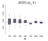
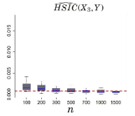
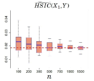
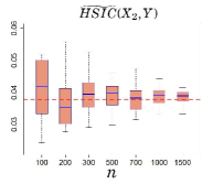
Figure 1: Convergence plots of the estimators $\widehat{\operatorname{HSIC}}(X_{k},Y)$ and $\widetilde{\operatorname{HSIC}}(X_{k},Y)$ for Ishigami function, according to the sample size $n$. Theoretical values are represented in red dashed lines.

On this same example, we are now interested in the classification of input variables by order of influence. For this, the sensitivity index $R^{2}_{\operatorname{HSIC},k}\;(1\leq k\leq d)$ is computed from $\widetilde{\operatorname{HSIC}}(X_{k},Y)$ with Equation (14) and the inputs are ordered by decreasing $\widetilde{R}^{2}_{\operatorname{HSIC},k}$. For each sample size, the rates of good ranking of inputs given by $\widetilde{\operatorname{R}2}^{2}_{\operatorname{HSIC}}$ estimators are also computed. Results are given in Table (1): they illustrate that, even for small sample sizes (e.g $n=200$), modified estimators $\widetilde{\operatorname{R}2}^{2}_{\operatorname{HSIC}}$ have good ranking ability.

$n=100$	$n=200$	$n=300$	$n\geqslant 500$
$88\%$	$93.5\%$	$97\%$	$100\%$

Table 1: Good ranking rates of input variables using modified estimators $\widetilde{\operatorname{R}2}^{2}_{\operatorname{HSIC}}$ for the Ishigami function, for different sample sizes $n$.

3 New methodology for second-level GSA

In this section, we first define the 2${}^{\text{nd}}$-level global sensitivity analysis (GSA2) before listing the issues raised by its implementation. We then present and detail the methodology that we propose, in order to tackle these issues.

3.1 Principle and objective

In this part, we assume that the inputs $X_{1},\ldots,X_{d}$ vary according to unknown probability distributions $\mathbb{P}_{X_{1}},\ldots,\mathbb{P}_{X_{d}}$. This lack of knowledge can take many forms; we mention as examples, the case of parameterized distributions where the parameters are unknown, or the case where the distribution characteristics (e.g. mean, variance, etc.) are known but not the nature of the law (uniform, triangular, normal, etc.). As part of a probabilistic approach, this lack of knowledge is modeled by probability laws (on a set of distributions) denoted $\mathbb{P}_{\mathbb{P}_{X_{1}}},\ldots,\mathbb{P}_{\mathbb{P}_{X_{d}}}$.

Each assumed joint distribution $\mathbb{P}_{X}=\mathbb{P}_{X_{1}}\times\ldots\times\mathbb{P}_{X_{d}}$ of inputs yields potentially different results of 1${}^{\text{st}}$-level global sensitivity analysis (GSA1). It is therefore important to take into account the impact of these uncertainties on GSA1 results. Thus, we will designate by GSA2 the statistical methods whose purpose is to quantify for each input parameter $X_{k}$, the impact of the uncertainty of $\mathbb{P}_{X_{k}}$ on GSA1 results, this uncertainty being modeled by $\mathbb{P}_{\mathbb{P}_{X_{k}}}$. From GSA2 results, the probability distributions of inputs can be separated into two groups: those which significantly modify GSA1 results and those whose influence is negligible. Subsequently, probability distributions with a small impact can be set to a reference law and the efforts of characterization will be focused on the most influential distributions to improve their knowledge (strategy of uncertainty reduction).

3.2 Issues raised by GSA2

We present in what follows the different issues and technical locks raised by the realization of a GSA2.

3.2.1 Characterization of GSA1 results

The realization of GSA2 requires a prior characterization of GSA1 results. This characterization consists in associating to a given input distribution $\mathbb{P}_{X}=\mathbb{P}_{X_{1}}\times\ldots\times\mathbb{P}_{X_{d}}$, a measurable quantity $\operatorname{\mathcal{R}}$ which represents GSA1 results. To choose this quantity of interest, we propose the following options, all based on HSIC (see 2.1.3):

• Vector $\mathbf{\operatorname{R}2^{2}_{\operatorname{HSIC}}}=(\operatorname{R}2^{2}_{\operatorname{HSIC},1},\ldots,\operatorname{R}2^{2}_{\operatorname{HSIC},d})$ of sensitivity indices. The quantity of interest $\operatorname{\mathcal{R}}=\mathbf{\operatorname{R}2^{2}_{\operatorname{HSIC}}}$ is thereby a vector of $d$ real components.

• Ranking of inputs $X_{1},\ldots,X_{d}$ using the indices $\operatorname{R}2^{2}_{\operatorname{HSIC},1},\ldots,\operatorname{R}2^{2}_{\operatorname{HSIC},d}$ . In this case, the quantity of interest $\operatorname{\mathcal{R}}$ is a permutation on the set $\{1,\ldots,d\}$, which verifies that $\operatorname{\mathcal{R}}(k)=j$ if and only if the variable $X_{j}$ is the $k$-th in the ranking.

• Vector $\mathbf{\operatorname{P}}=(\operatorname{P_{1}}1,\ldots,\operatorname{P_{d}})$ of p-values associated with asymptotic independence tests. In this case, the quantity of interest $\operatorname{\mathcal{R}}=\mathbf{\operatorname{P}}$ is a vector of $d$ components in $[0,1]^{d}$.

• Vector $\mathbf{\operatorname{p}}=(\operatorname{p_{1}}1,\ldots,\operatorname{p_{d}})$ of p-values associated with permutation independence tests. The quantity of interest $\operatorname{\mathcal{R}}=\mathbf{\operatorname{p}}$ is a vector of $d$ components in $[0,1]^{d}$.

3.2.2 Definition of 2${}^{\text{nd}}$-level sensitivity indices

By analogy with formulas (2), it is possible to build 2${}^{\text{nd}}$-level HSIC measures between the probability distributions $\mathbb{P}_{X_{1}},\ldots,\mathbb{P}_{X_{d}}$ and the quantity of interest $\operatorname{\mathcal{R}}$. This involves to define RKHS kernels $l_{\operatorname{\mathcal{D}_{1}}1},\ldots,l_{\operatorname{\mathcal{D}_{d}}}$ on input distributions and a RKHS kernel $l_{\operatorname{\mathcal{R}}}$ on the quantity of interest $\operatorname{\mathcal{R}}$. This point will be further detailed in Section 3.4. Thus, assuming all the kernels are defined, we propose the 2${}^{\text{nd}}$-level HSIC measures defined for $k=1..d$ by:

$$\operatorname{HSIC}(\mathbb{P}_{X_{k}},\operatorname{\mathcal{R}}) =\mathbb{E}\left[l_{\operatorname{\mathcal{D}_{k}}}(\mathbb{P}_{X_{k}},\mathbb{P}^{\prime}_{X_{k}})l_{\operatorname{\mathcal{R}}}(\operatorname{\mathcal{R}},\operatorname{\mathcal{R}}^{\prime})\right]+\mathbb{E}\left[l_{\operatorname{\mathcal{D}_{k}}}\left(\mathbb{P}_{X_{k}},\mathbb{P}^{\prime}_{X_{k}}\right)\right]\mathbb{E}\left[l_{\operatorname{\mathcal{R}}}\left(\operatorname{\mathcal{R}},\operatorname{\mathcal{R}}^{\prime}\right)\right]$$

$$-2\mathbb{E}\left[\mathbb{E}\left[l_{\operatorname{\mathcal{D}_{k}}}\left(\mathbb{P}_{X_{k}},\mathbb{P}^{\prime}_{X_{k}}\right)\mid\mathbb{P}_{X_{k}}\right]\mathbb{E}\left[l_{\operatorname{\mathcal{R}}}\left(\operatorname{\mathcal{R}},\operatorname{\mathcal{R}}^{\prime}\right)\mid\operatorname{\mathcal{R}}\right]\right],$$ (19)

where $\mathbb{P}^{\prime}_{X_{k}}$ is an independent and identically distributed copy of $\mathbb{P}_{X_{k}}$ and $\operatorname{\mathcal{R}}^{\prime}$ the GSA1 results associated to $\mathbb{P}^{\prime}_{X_{k}}$.

From 2${}^{\text{nd}}$-level HSIC measures, we can define GSA2 indices by:

$$\operatorname{R}2^{2}_{\operatorname{HSIC}}(\mathbb{P}_{X_{k}},\operatorname{\mathcal{R}})=\displaystyle\frac{\operatorname{HSIC}(\mathbb{P}_{X_{k}},\operatorname{\mathcal{R}})}{\sqrt{\operatorname{HSIC}(\mathbb{P}_{X_{k}},\mathbb{P}_{X_{k}})\operatorname{HSIC}(\operatorname{\mathcal{R}},\operatorname{\mathcal{R}})}},\;\text{for}\;k=1..d.$$ (20)

3.2.3 Monte Carlo estimation

To estimate $\operatorname{R}2^{2}_{\operatorname{HSIC}}(\mathbb{P}_{X_{k}},\operatorname{\mathcal{R}})$, for $k=1..d$, one has to dispose of a $n_{1}$-sized sample $(\mathbb{P}^{(i)}_{\mathbf{X}},\mathcal{R}^{(i)})_{1\leq i\leq n_{1}}$ of $(\mathbb{P}_{\mathbf{X}},\mathcal{R})$. For this, we could consider a double loop Monte Carlo approach. In the outer loop, at each iteration $i$, a distribution $\mathbb{P}^{(i)}_{\mathbf{X}}$ is randomly generated from $\mathbb{P}_{\mathbb{P}_{X}}=\mathbb{P}_{\mathbb{P}_{X_{1}}}\times\ldots\times\mathbb{P}_{\mathbb{P}_{X_{d}}}$. The quantity of interest $\mathcal{R}^{(i)}$ associated to this distribution $\mathbb{P}^{(i)}_{\mathbf{X}}$ is provided by a 2^nd loop. This inner loop consists in generating a $n_{2}$-sized sample $(X_{1}^{(i,j)},\ldots,X_{d}^{(i,j)})_{1\leq j\leq n_{2}}$ where $\mathbf{X}$ follows $\mathbb{P}^{(i)}_{\mathbf{X}}$. The $n_{2}$ corresponding outputs $(Y^{(i,j)})_{1\leq j\leq n_{2}}$ are computed in this inner loop. Once this loop performed, the quantity of interest $\mathcal{R}^{(i)}$ is computed from $\mathcal{E}^{(i)}=(X_{1}^{(i,j)},\ldots,X_{d}^{(i,j)},Y^{(i,j)})_{1\leq j\leq n_{2}}$. This process is repeated for each $\mathbb{P}^{(i)}_{\mathbf{X}}$ of the outer loop. At the end, 2^nd-level HSIC can be estimated from the sample $(\mathbb{P}^{(i)}_{\mathbf{X}},\mathcal{R}^{(i)})_{1\leq i\leq n_{1}}$ by:

$$\widehat{\operatorname{HSIC}}(\mathbb{P}_{X_{k}},\mathcal{R})=\displaystyle\frac{1}{n_{1}^{2}}Tr(L_{\operatorname{\mathcal{D}_{k}}}HL_{\mathcal{R}}H),$$ (21)

where $L_{\operatorname{\mathcal{D}_{k}}}$ and $L_{\mathcal{R}}$ are the matrices defined for all $(i,j)\in\{1,\ldots,n_{1}\}$ by: $(L_{\operatorname{\mathcal{D}_{k}}})_{i,j}=l_{\operatorname{\mathcal{D}_{k}}}(\mathbb{P}^{(i)}_{X_{k}},\mathbb{P}^{(j)}_{X_{k}})$, $(L_{\mathcal{R}})_{i,j}=l_{\mathcal{R}}\left(\mathcal{R}^{(i)},\mathcal{R}^{(j)}\right)$ and $H$ the matrice defined in Formula (5).

From 2${}^{\text{nd}}$-level HSIC estimators, 2${}^{\text{nd}}$-level $\operatorname{R}2^{2}_{\operatorname{HSIC}}$ indices can be estimated using plug-in and Formula (21) by:

$$\widehat{\operatorname{R}2}^{2}_{\operatorname{HSIC}}(\mathbb{P}_{X_{k}},\mathcal{R})=\displaystyle\frac{\widehat{\operatorname{HSIC}}(\mathbb{P}_{X_{k}},\mathcal{R})}{\sqrt{\widehat{\operatorname{HSIC}}(\mathbb{P}_{X_{k}},\mathbb{P}_{X_{k}})\widehat{\operatorname{HSIC}}(\mathcal{R},\mathcal{R})}}.$$ (22)

Consequently, this Monte Carlo double-loop approach requires a total of $n_{1}n_{2}$ code simulations. For example, if $n_{1}=100$ and $n_{2}=1000$, the computation of 2^nd-level sensitivity indices HSIC requires $10^{5}$ code calls. This approach is therefore not tractable for CPU-time expensive simulators.

To overcome this problem and reduce the number of code-calls, we propose a single-loop Monte Carlo approach to obtain the sample $(\mathbb{P}^{(i)}_{\mathbf{X}},\mathcal{R}^{(i)})_{1\leq i\leq n_{1}}$, which requires only $n_{2}$ simulations, and allows to consider a large sample $\mathcal{P}$ of distributions $\mathbb{P}_{\mathbf{X}}$. This new algorithm is detailed in the next section.

3.3 Algorithm for computing 2${}^{\text{nd}}$-level sensitivity indices with a single Monte Carlo loop

In this part, we detail the algorithm to estimate the 2${}^{\text{nd}}$-level HSIC (and $\operatorname{R}2^{2}_{\operatorname{HSIC}}$) from a unique inputs/output sample $\mathcal{E}$. We assume that inputs are generated from a unique and known probability distribution denoted $\overline{\mathbb{P}}_{\mathbf{X}}=\overline{\mathbb{P}}_{X_{1}}\times\ldots\times\overline{\mathbb{P}}_{X_{d}}$ with density denoted $\overline{f}(x_{1},\ldots,x_{d})=\overline{f}_{1}(x_{1})\times\ldots\times\overline{f}_{d}(x_{d})$. The options for choosing $\overline{f}$ will be discussed in Section 3.5. The algorithm consists of 3 steps:

• Step 1. Build a unique $n_{2}$-sized sample $\mathcal{E}$ from $\overline{f}$

  In this step, we first draw a sample $\overline{\mathbf{X}}=\left(\mathbf{X}^{(i)}\right)_{1\leq i\leq n_{2}}$ according to $\overline{f}$, then we compute the associated outputs $\overline{Y}=\left(Y^{(i)}\right)_{1\leq i\leq n_{2}}$, to obtain a sample $\mathcal{E}=(\overline{\mathbf{X}},\overline{Y})$ of inputs/output. Thus, in what follows, all the formulas for modified HSIC will be used with the alternative sample $\mathcal{E}$, $\overline{f}$ being the alternative distribution. Hence, in all the modified HSIC formulas, the alternative sample will be $(\widetilde{\mathbf{X}},\widetilde{Y})=(\overline{\mathbf{X}},\overline{Y})$.

• Step 2. Perform $n_{1}$ GSA1 from $\mathcal{E}$

  First, we generate a $n_{1}$-sized sample of input distributions according to $\mathbb{P}_{\mathbb{P}_{\mathbf{X}}}$. This sample of distributions is denoted $\mathcal{P}=\left(\mathbb{P}_{\mathbf{X}}^{(i)}\right)_{1\leq i\leq n_{1}}$ and the density associated to each distribution $\mathbb{P}_{\mathbf{X}}^{(i)}$ is denoted $f^{(i)}=(f^{(i)}_{1},\ldots,f^{(i)}_{d})$. The objective is then to compute the GSA1 results $\mathcal{R}^{(i)}$ associated to each distribution $\mathbb{P}_{\mathbf{X}}^{(i)}$, using only $\mathcal{E}$. The options proposed for $\mathcal{R}^{(i)}$ in Section 3.2.1 are distinguished:

  • Vector $\mathcal{R}^{(i)}=(\operatorname{R}2^{2,(i)}_{\operatorname{HSIC},1},\ldots,\operatorname{R}2^{2,(i)}_{\operatorname{HSIC},d})$ of sensitivity indices. In this case, each $\operatorname{R}2^{2,(i)}_{\operatorname{HSIC}}$ is estimated by $\widetilde{\operatorname{R}2}^{2}_{\operatorname{HSIC},k}$ given by Equation (14) with $\mathcal{E}=(\overline{\mathbf{X}},\overline{Y})$.

  • Ranking of inputs $X_{1},\ldots,X_{d}$ using the indices $\operatorname{R}2^{2}_{\operatorname{HSIC},1},\ldots,\operatorname{R}2^{2}_{\operatorname{HSIC},d}$ . These rankings are obtained by ordering the coordinates of $\widetilde{\operatorname{R}2}^{2}_{\operatorname{HSIC}}$ vectors; still estimated from $\mathcal{E}$ and Equation (14).

  • Vector $\mathcal{R}^{(i)}=(\operatorname{P}_{1}^{(i)},\ldots,\operatorname{P}_{d}^{(i)})$ of p-values associated with asymptotic independence tests. By analogy with Equation (8), each $\operatorname{P}_{k}^{(i)}$ is estimated thanks to the properties of the modified estimators:

    $$\widetilde{\operatorname{P}}_{k}^{(i)}\simeq 1-\widetilde{\operatorname{F}}_{\operatorname{G_{k}}}\left(n_{2}\times\widetilde{\operatorname{HSIC}}(X_{k}^{(i)},Y)_{obs}\right),\;k=1,\ldots,d$$ (23)

    where $\tilde{\operatorname{F}}_{\operatorname{G_{k}}}$ is the cumulative distribution function of Gamma law approximating the asymptotic law of $n_{2}\times\widetilde{\operatorname{HSIC}}(X_{k}^{(i)},Y)$.

  • Vector $\mathcal{R}^{(i)}=(\operatorname{p}_{1}^{(i)},\ldots,\operatorname{p}_{d}^{(i)})$ of p-values associated with permutation independence tests. Using the same notations as in Formula (9), each $\operatorname{p}_{k}^{(i)}$ is estimated by:

    $$\widetilde{\operatorname{p}}_{k}^{(i)}=\displaystyle\frac{1}{B}\sum_{b=1}^{B}\mathds{1}_{\widetilde{\operatorname{HSIC}}^{[b]}(X_{k}^{(i)},Y)>\widetilde{\operatorname{HSIC}}(X_{k}^{(i)},Y)},\;k=1,\ldots,d.$$ (24)

• Step 3. Estimate 2${}^{\text{nd}}$-level sensitivity indices

  Finally, the 2${}^{\text{nd}}$-level sensitivity indices $\operatorname{R}2^{2}_{\operatorname{HSIC}}(\mathbb{P}_{X_{k}},\operatorname{\mathcal{R}})$ are estimated with the sample $(\mathbb{P}^{(i)}_{\mathbf{X}},\widetilde{\mathcal{R}}^{(i)})_{1\leq i\leq n_{1}}$ using Formulas (21) and (22). The computation of matrices $L_{\operatorname{\mathcal{D}_{k}}},\;k=1,\ldots,d$ and $L_{\mathcal{R}}$ requires the definition of specific RKHS kernels $l_{\operatorname{\mathcal{D}_{k}}},\;k=1,\ldots,d$ and $l_{\mathcal{R}}$. This item is detailed in the next section.

3.4 Choice of characteristic kernels for probability distributions and for quantities of interest

In this part, we present examples of characteristic RKHS kernels for probability distributions and for the different quantities of interest $\mathcal{R}$, these kernels being involved in Formula (21) (and as a result in Equation (22)).

Characteristic RKHS kernel for probability distributions. Before defining a characteristic kernel for distributions, we first introduce the Maximum Mean Discrepancy (MMD) defined in [21]. If we consider two distributions $\mathbb{P}_{1}$ and $\mathbb{P}_{2}$ having the same support and if $K$ denotes a RKHS kernel defined on the commun support of $\mathbb{P}_{1}$ and $\mathbb{P}_{2}$, then the MMD between $\mathbb{P}_{1}$ and $\mathbb{P}_{2}$ induced by $K$ is defined as:

$$\text{MMD}_{K}(\mathbb{P}_{1},\mathbb{P}_{2})=\mathbb{E}[K(Z_{1},Z^{\prime}_{1})]-2\mathbb{E}[K(Z_{1},Z_{2})]+\mathbb{E}[K(Z_{2},Z^{\prime}_{2})],$$ (25)

where $Z_{1}$, $Z_{2}$ are random variables respectively with laws $\mathbb{P}_{1}$, $\mathbb{P}_{2}$ and $Z^{\prime}_{1}$, $Z^{\prime}_{2}$ are independent and identically distributed copies respectively of $Z_{1}$, $Z_{2}$.

Authors of [21] establish that when $K$ is characteristic, the MMD associated to $K$ defines a distance. From MMD distance, [39] defines Gaussian RKHS kernels between probability distributions in a similar way to Formula (3):

$$l_{\mathcal{D}}(\mathbb{P}_{1},\mathbb{P}_{2})=\exp\left(-\lambda\operatorname{MMD}^{2}_{K}(\mathbb{P}_{1},\mathbb{P}_{2})\right),$$ (26)

where $\lambda$ is a positive real parameter.

It has been shown in [7] that when the commun support of distributions is compact, the Gaussian MMD-based kernel is universal (and consequently characteristic). We can then define kernels $l_{\operatorname{\mathcal{D}_{k}}},\;k=1,\ldots,d$ introduced in Formula (19) by:

$$l_{\operatorname{\mathcal{D}_{k}}}(\mathbb{P}_{X_{k}},\mathbb{P}_{X^{\prime}_{k}})=\exp\left(-\lambda_{k}\operatorname{MMD}_{l_{k}}^{2}(\mathbb{P}_{X_{k}},\mathbb{P}_{X^{\prime}_{k}})\right),$$ (27)

where $\lambda_{k},\;k=1,\ldots,d$ are positive real parameters.

From a practical point of view, one can choose $\lambda_{k}$ as the inverse of $s_{k}^{2}$, the empirical variance w.r.t MMD distance (i.e. $\lambda_{k}=1/s_{k}^{2}$):

$$s^{2}_{k}=\displaystyle\frac{1}{n_{1}^{2}}\sum_{i=1}^{n_{1}}\operatorname{MMD}_{l_{k}}^{2}\left(\mathbb{P}^{(i)}_{X_{k}},\overline{\mathbb{P}}_{X_{k}}\right),$$

where the distribution $\overline{\mathbb{P}}_{X_{k}}$ is defined as, $\overline{\mathbb{P}}_{X_{k}}=\displaystyle\frac{1}{n_{1}}\sum_{i=1}^{n_{1}}\mathbb{P}^{(i)}_{X_{k}}$.

Characteristic RKHS kernel for permutations as quantity of interest. When GSA1 results $\mathcal{R}$ is a permutation (see Section 3.2.1), we propose to use Mallows kernel $K_{M}$ [27], the Mallows kernel is universal (and characteristic) [31]. This kernel is given, for two permutations $\sigma$, $\sigma^{\prime}$ by:

$$K_{M}(\sigma,\sigma^{\prime})=\exp\left(-\lambda n_{d}(\sigma,\sigma^{\prime})\right),$$ (28)

where $\lambda$ is a positive real parameter and $n_{d}$ is the number of discordant pairs between $\sigma$ and $\sigma^{\prime}$:

$$n_{d}(\sigma,\sigma^{\prime})=\displaystyle\sum_{1\leq r<s\leq d}\left[\mathds{1}_{\{\sigma(r)<\sigma(s)\}}\mathds{1}_{\{\sigma^{\prime}(r)>\sigma^{\prime}(s)\}}+\mathds{1}_{\{\sigma(r)>\sigma(s)\}}\mathds{1}_{\{\sigma^{\prime}(r)<\sigma^{\prime}(s)\}}\right].$$ (29)

In practice, if a $n_{1}$-sample of $\sigma$ is available, we propose to choose $\lambda$ as the inverse of the empirical mean of $n_{d}(\sigma,\sigma^{\prime})$.

Characteristic RKHS kernel for real vectors as quantities of interest. In cases where $\mathcal{R}$ is a vector of $\mathbb{R}^{d}$, the usual Gaussian kernel defined in Formula (3) can be considered.

3.5 Possibilities for the unique sampling distribution

We propose three different possibilities for the single draw density $\overline{f}(x_{1},\ldots,x_{d})=\overline{f}_{1}(x_{1})\times\ldots\times\overline{f}_{d}(x_{d})$ which is used to generate the unique sample $\mathcal{E}$ in Step 1 of the algorithm (Section 3.3). Note here that the support of each $\overline{f}_{k},\;k=1,\ldots,d$ must be $\mathcal{X}_{k}$ (the variation domain of $X_{k}$, see Section 2). To have a density $\overline{f}_{k}$ close to the set of all possible densities and more particularly to the most likely ones, we propose to use either mixture distribution or two barycenter distributions, namely the Wasserstein barycenter and the symmetric Kullback-Leibler barycenter.

Option 1: mixture distribution. The mixture density $\overline{f}_{M}$ (see e.g. [17, 43]) of a random density probability $f$ is defined by:

$$\overline{f}_{M}=\displaystyle\mathbb{E}_{\mathbb{F}}\left[f\right]=\displaystyle\int_{\mathcal{F}}f\;\mathrm{d}\mathbb{F}(f),$$ (30)

with $f$ lying in $\mathcal{F}$ with probability distribution measure $\mathrm{d}\mathbb{F}$.

If $\mathbb{F}$ is discrete over a finite parametric set $\{f_{\theta_{0}},\ldots,f_{\theta_{m}}\}$, the mixture density is written as

$$\overline{f}_{M}=\displaystyle\sum_{r=0}^{m}f_{\theta_{r}}\;\mathbb{F}(f_{\theta_{r}}).$$ (31)

If the density $f$ depends on a parameter which is generated according to a continuous density $\pi$ over $\Theta$, the mixture density is defined by

$$\overline{f}_{M}=\displaystyle\int_{\Theta}f_{\theta}\;\pi(\theta)\;d\theta.$$ (32)

Option 2: symmetrized Kullback-Leibler barycenter. The symmetric Kullback-Leibler distance [28] is a distance obtained by symmetrizing the Kullback-Leibler divergence. It is defined for two real distributions $\mu$ and $\nu$ by:

$$D^{S}_{K}(\mu,\nu)=\displaystyle\frac{1}{2}\big{(}KL(\mu||\nu)+KL(\nu||\mu)\big{)},$$ (33)

where $KL(Q_{1}||Q_{2})=\displaystyle\int log(\frac{dQ_{1}}{dQ_{2}})dQ_{1}$ is the Kullback-Leibler divergence.

For of a finite set of unidimensional and equiprobable densities $\{f_{1},\ldots,f_{m}\}$, the symmetrized Kullback-Leibler barycenter $\overline{f}_{K}$ can not directly be expressed using densities. However, the distribution $Q_{K}$ of density $\overline{f}_{K}$ defined by:

$$\overline{f}_{K}=\displaystyle\frac{1}{2m}\sum_{r=1}^{m}f_{r}+\displaystyle\frac{\displaystyle\left(\prod_{r=1}^{m}f_{r}\right)^{\frac{1}{m}}}{\displaystyle 2\int\left(\prod_{r=1}^{m}f_{r}\right)^{\frac{1}{m}}},$$ (34)

is a very good approximation of symmetrized Kullback-Leibler barycenter (see [44] for detailed proofs).

To generalize the Formula (34) to a probabilistic set of one-dimensional densities, we propose:

$$\overline{f}_{K}=\displaystyle\frac{1}{2}\mathbb{E}_{\mathbb{F}}\left[f\right]+\displaystyle\frac{\displaystyle e^{\mathbb{E}_{\mathbb{F}}\left[lnf\right]}}{\displaystyle 2\int e^{\mathbb{E}_{\mathbb{F}}\left[lnf\right]}}.$$ (35)

where $\mathbb{E}_{\mathbb{F}}\left[f\right]$ and $\mathbb{E}_{\mathbb{F}}\left[lnf\right]$ are mixture functions of random functions $f$ and $lnf$ (given by Equation (30)).

Option 3: Wasserstein barycenter distribution. The Wasserstein distance (see e.g. [20, 45]) of order $p$ between two real distributions $\mu$ and $\nu$ with the same support $A$ is defined by:

$$W_{p}(\mu,\nu)=\left(\inf\limits_{\gamma\in\Gamma(\mu,\nu)}\int_{A\times A}|x-y|^{p}\,\mathrm{d}\gamma(x,y)\right)^{1/p},$$ (36)

where $\Gamma(\mu,\nu)$ is the set of probability measures on $A\times A$ with marginals $\mu$ and $\nu$.

Note that in the general case, when referring to the Wasserstein distance (without specifying the order) we refer to Wasserstein distance of order 2.

For a finite set $\mathcal{F}$ of unidimensional and equiprobable densities, the Wasserstein barycenter density [1] is the one whose quantile function is the mean of the quantile functions of the elements of the set $\mathcal{F}$:

$$\overline{q}_{W}=\displaystyle\frac{1}{|\mathcal{F}|}\sum_{f\in\mathcal{F}}\;q_{f},$$ (37)

where $\overline{q}_{W}$ denotes the quantile function of Wasserstein barycenter, $|\mathcal{F}|$ the cardinal of the set $\mathcal{F}$ and $q_{f}$ the quantile function associated to $f$.

To generalize Formula (37) to a probabilistic set of one-dimensional densities, we propose to use:

$$\overline{q}_{W}=\mathbb{E}_{\mathbb{F}}[q_{f}],$$ (38)

where $\mathbb{E}_{\mathbb{F}}[q_{f}]$ is the mixture quantile function of the quantile functions $\left(q_{f}\right)_{f\in\mathcal{F}}$.

4 Application of GSA2 methodology

In this part, our proposed methodology is first applied to an analytical model. The three different options proposed in Section 3.5 to genarate the unique sample are studied and compared. Moreover, the benefit of this new methodology comparing to a "double loop" approach is highlighted. Thereafter, the whole methodology is applied to a nuclear study case simulating a severe nuclear reactor accident.

4.1 Analytical example

Our proposed "single loop" methodology for GSA2 is first tested on the analytical model presented in Section 2.2.3. We recall that this model is defined on the set $[0,1]^{3}$ by $h(X_{1},X_{2},X_{3})=\sin(X_{1})+1.5\;\sin^{2}(X_{2})+0.5\;X_{3}^{4}\;\sin(X_{1})$. The inputs $X_{1}$, $X_{2}$ and $X_{3}$ are assumed here to be independent and their probability distributions $\mathbb{P}_{X_{1}}$, $\mathbb{P}_{X_{2}}$ et $\mathbb{P}_{X_{3}}$ can equiprobably be the laws $\mathbb{P}_{U}$, $\mathbb{P}_{T}$ et $\mathbb{P}_{N}$, where

• $\mathbb{P}_{U}$ is the uniform distribution on $[0,1]$,

• $\mathbb{P}_{T}$ is the triangular distribution on $[0,1]$ with mode $0.4$,

• $\mathbb{P}_{N}$ is the truncated normal distribution on $[0,1]$ with mean $0.6$ and standard deviation $0.2$.

We want here to estimate from a single inputs/output sample, the 2${}^{\text{nd}}$-level GSA indices $\operatorname{R}2^{2}_{\operatorname{HSIC}}(\mathbb{P}_{X_{k}},\operatorname{\mathcal{R}})_{k=1\ldots d}$ indices of the model $Y=h(\mathbf{X})$ for different sample sizes. For this, we use HSIC measures for GSA1 (and $\operatorname{R}2^{2}_{\operatorname{HSIC}}(X_{k},Y)_{k=1\ldots d}$ indices) with standardized Gaussian kernel. We characterize GSA1 results by the vector of 1${}^{\text{st}}$-level $\operatorname{R}2^{2}_{\operatorname{HSIC}}$ (option 1 in Section 3.3). To compute the 2${}^{\text{nd}}$-level $\operatorname{R}2^{2}_{\operatorname{HSIC}}$ indices, MMD-based kernels $l_{\operatorname{\mathcal{D}_{k}}}$ (Equation 26) are used for input distributions and the standardized Gaussian kernel (Equation 3) is used for GSA1 results.

Remark 4.1.

The other quantities of interest characterizing GSA1 results could be studied in a similar way.

4.1.1 Computation of theorical values

In order to compute theoretical values of 2${}^{\text{nd}}$-level HSIC and $\operatorname{R}2^{2}_{\operatorname{HSIC}}$ indices, we consider the finite set of the $n_{1}=27$ possible triplet of input probability distributions. The 1${}^{\text{st}}$-level $\operatorname{R}2^{2}_{\operatorname{HSIC}}$ vector associated to each distribution is then computed with a sample of size $n_{2}=1000$ (which ensures the convergence of HSIC estimators). Theorical values of 2${}^{\text{nd}}$-level HSIC are estimated with Formula (21):

• $\operatorname{HSIC}(\mathbb{P}_{X_{1}},\mathcal{R})=0.0414$,

• $\operatorname{HSIC}(\mathbb{P}_{X_{2}},\mathcal{R})=0.0261$,

• $\operatorname{HSIC}(\mathbb{P}_{X_{3}},\mathcal{R})=0.0009$.

The theorical values of 2${}^{\text{nd}}$-level $\operatorname{R}2^{2}_{\operatorname{HSIC}}(\mathbb{P}_{X_{k}},\operatorname{\mathcal{R}})$ indices can also be computed:

• $\operatorname{R}2^{2}_{\operatorname{HSIC}}(\mathbb{P}_{X_{1}},\mathcal{R})=0.4152$,

• $\operatorname{R}2^{2}_{\operatorname{HSIC}}(\mathbb{P}_{X_{2}},\mathcal{R})=0.2516$,

• $\operatorname{R}2^{2}_{\operatorname{HSIC}}(\mathbb{P}_{X_{3}},\mathcal{R})=0.0086$.

We observe that $\operatorname{R}2^{2}_{\operatorname{HSIC}}(\mathbb{P}_{X_{1}},\mathcal{R})$ is considerably larger than $\operatorname{R}2^{2}_{\operatorname{HSIC}}(\mathbb{P}_{X_{2}},\mathcal{R})$, while $\operatorname{R}2^{2}_{\operatorname{HSIC}}(\mathbb{P}_{X_{3}},\mathcal{R})$ is negligible compared to the other two. In this example, the lack of knowledge on $\mathbb{P}_{X_{3}}$ has therefore no influence on 1${}^{\text{st}}$-level $\operatorname{R}2^{2}_{\operatorname{HSIC}}$. Furthermore, the uncertainty on $\mathbb{P}_{X_{1}}$ has a much higher impact than the one of $\mathbb{P}_{X_{2}}$, which remains non-negligible. Consequently, characterization efforts must be targeted in priority on $\mathbb{P}_{X_{1}}$, followed-up by $\mathbb{P}_{X_{2}}$.

4.1.2 GSA2 with our single loop approach

In the following, $\widetilde{\operatorname{HSIC}}_{M}(\mathbb{P}_{X_{k}},\mathcal{R})$, $\widetilde{\operatorname{HSIC}}_{W}(\mathbb{P}_{X_{k}},\mathcal{R})$ and $\widetilde{\operatorname{HSIC}}_{K}(\mathbb{P}_{X_{k}},\mathcal{R})$, $k=1,\ldots,3$ denote the 2${}^{\text{nd}}$-level HSIC measures respectively associated to mixture law, Wasserstein barycenter law and symmetrized Kullback-Leibler barycenter law. Similarly, $\widetilde{\operatorname{R}2}^{2}_{\operatorname{HSIC},\operatorname{M}}(\mathbb{P}_{X_{k}},\mathcal{R})$, $\widetilde{\operatorname{R}2}^{2}_{\operatorname{HSIC},\operatorname{W}}(\mathbb{P}_{X_{k}},\mathcal{R})$ and $\widetilde{\operatorname{R}2}^{2}_{\operatorname{HSIC},\operatorname{K}}(\mathbb{P}_{X_{k}},\mathcal{R}),k=1,\ldots,3$ are the derived 2${}^{\text{nd}}$-level $\operatorname{R}2^{2}_{\operatorname{HSIC}}$ indices.

In this section, we apply the methodology proposed in Section 3.3 to estimate GSA2 HSIC-based indices. For this, we consider Monte Carlo samples of sizes $n_{2}=100$ to $n_{2}=1500$. The estimations are repeated independently 200 times from independent samples. The results obtained with the three modified laws are given by Figure 2. The theoretical values of $\operatorname{R}2^{2}_{\operatorname{HSIC}}(\mathbb{P}_{X_{k}},\mathcal{R})$ are represented in dotted lines. In this case, the estimators $\widetilde{\operatorname{R}2}^{2}_{\operatorname{HSIC},\operatorname{M}}(\mathbb{P}_{X_{k}},\mathcal{R})$ and $\widetilde{\operatorname{R}2}^{2}_{\operatorname{HSIC},\operatorname{K}}(\mathbb{P}_{X_{k}},\mathcal{R})$ seem to have similar behaviors for both small and higher sample sizes. The dispersion of these two estimators remains high for small sizes (especially for $n_{2}\leq 200$) and becomes satisfying from $n_{2}=700$. The estimators $\widetilde{\operatorname{R}2}^{2}_{\operatorname{HSIC},\operatorname{W}}(\mathbb{P}_{X_{k}},\mathcal{R})$ have a higher variance than the two previous estimators, particularly for small and medium sample sizes ($300\leq n_{2}\leq 700$).

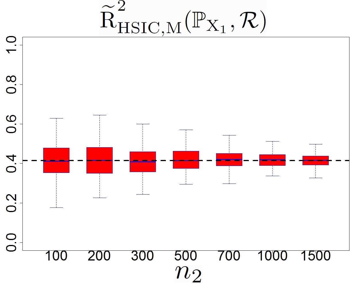
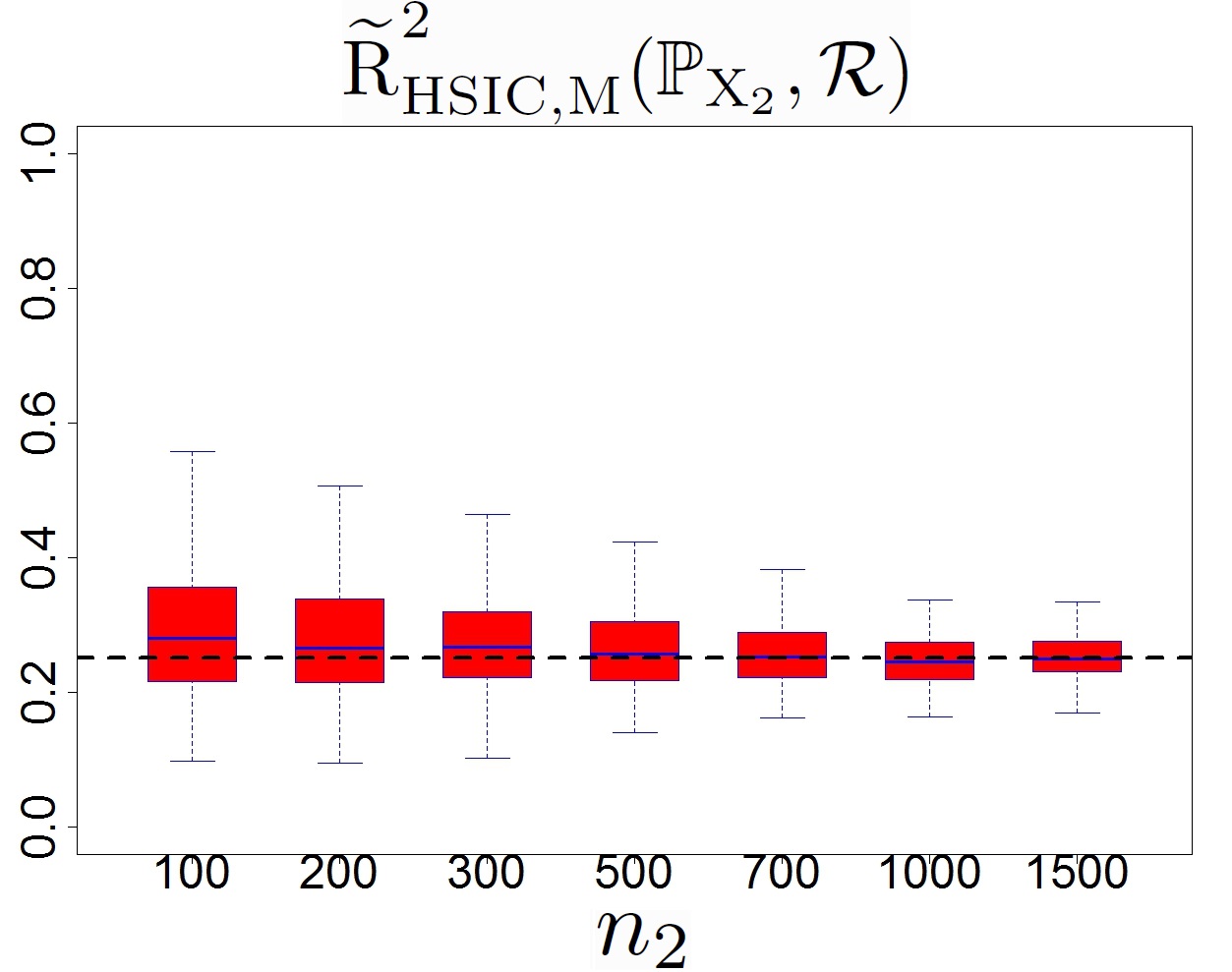
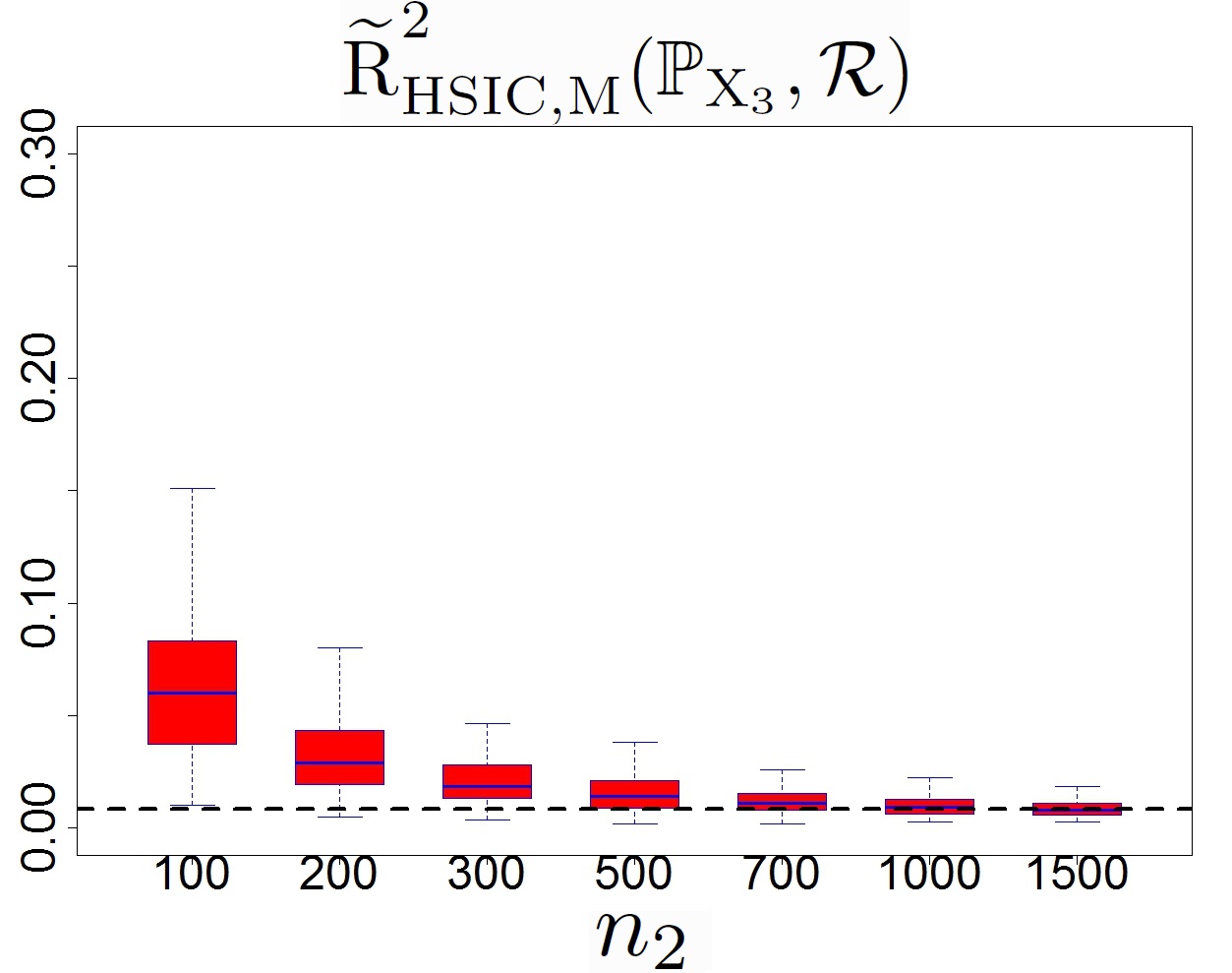
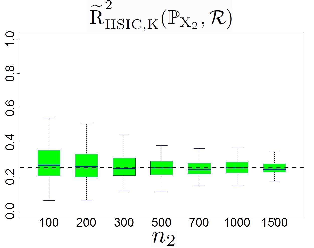
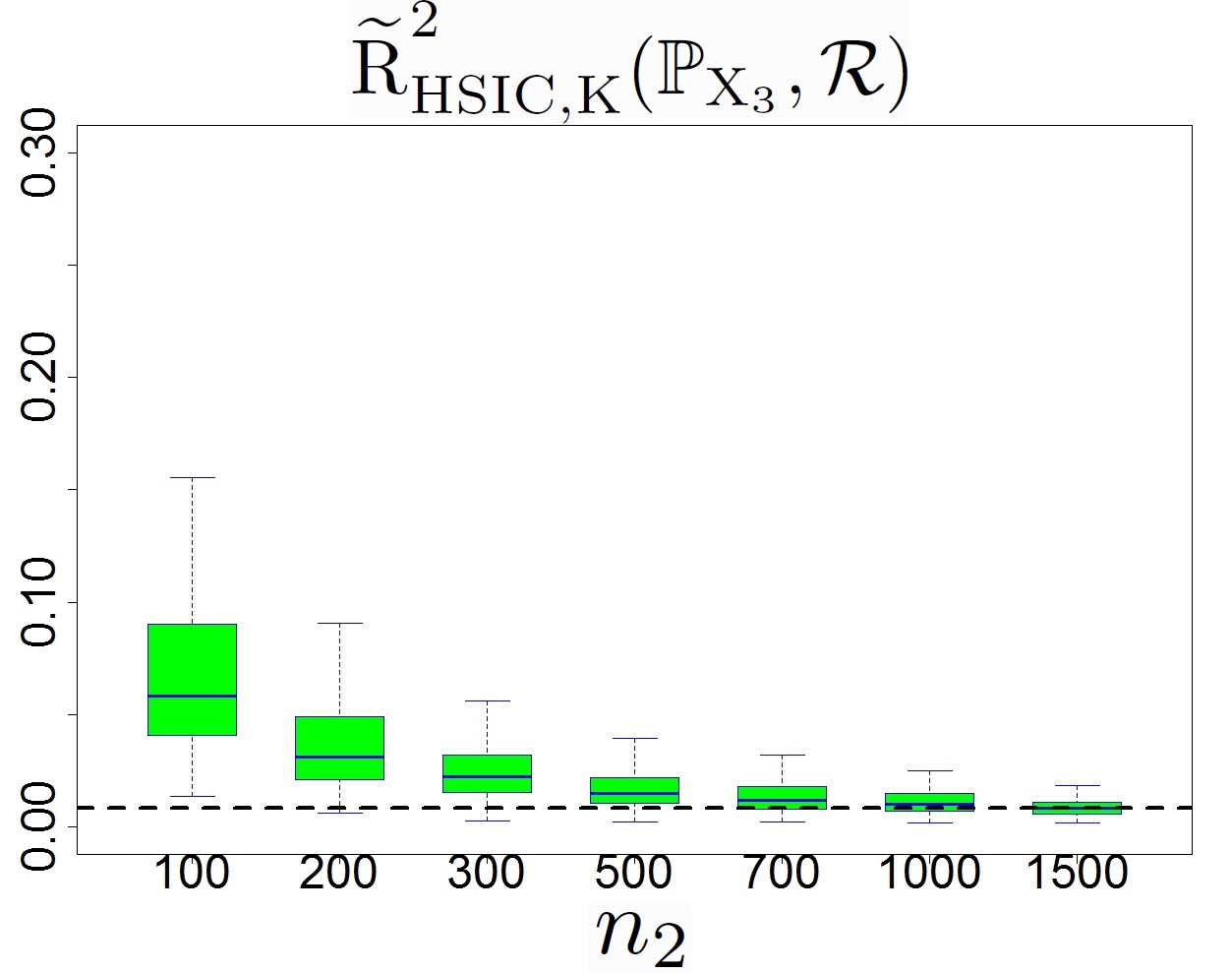
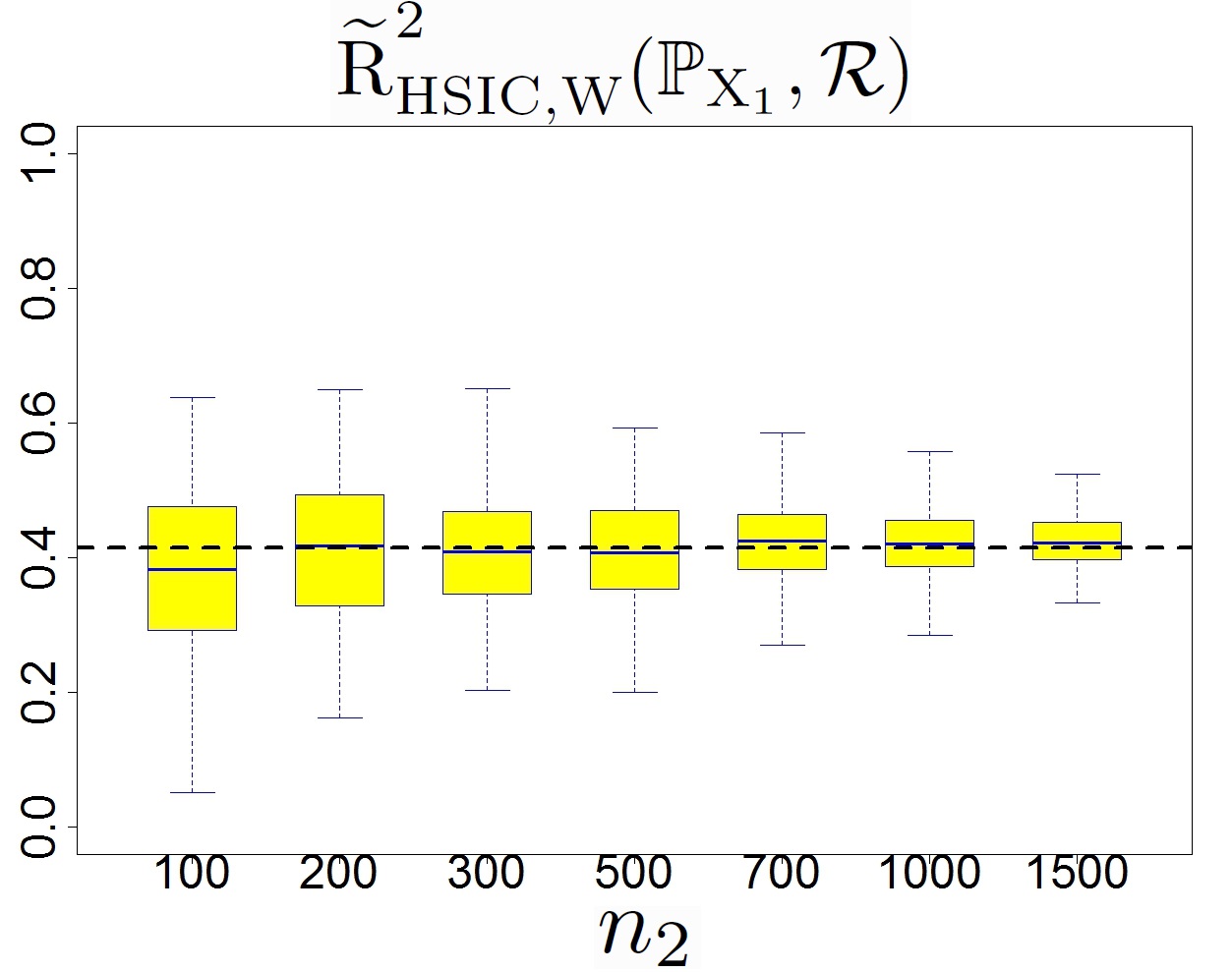
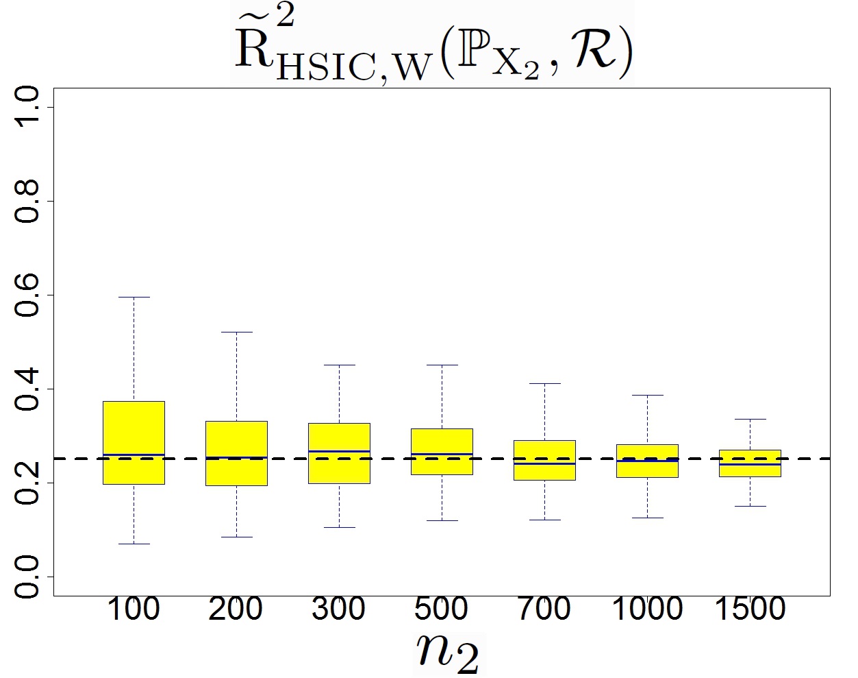
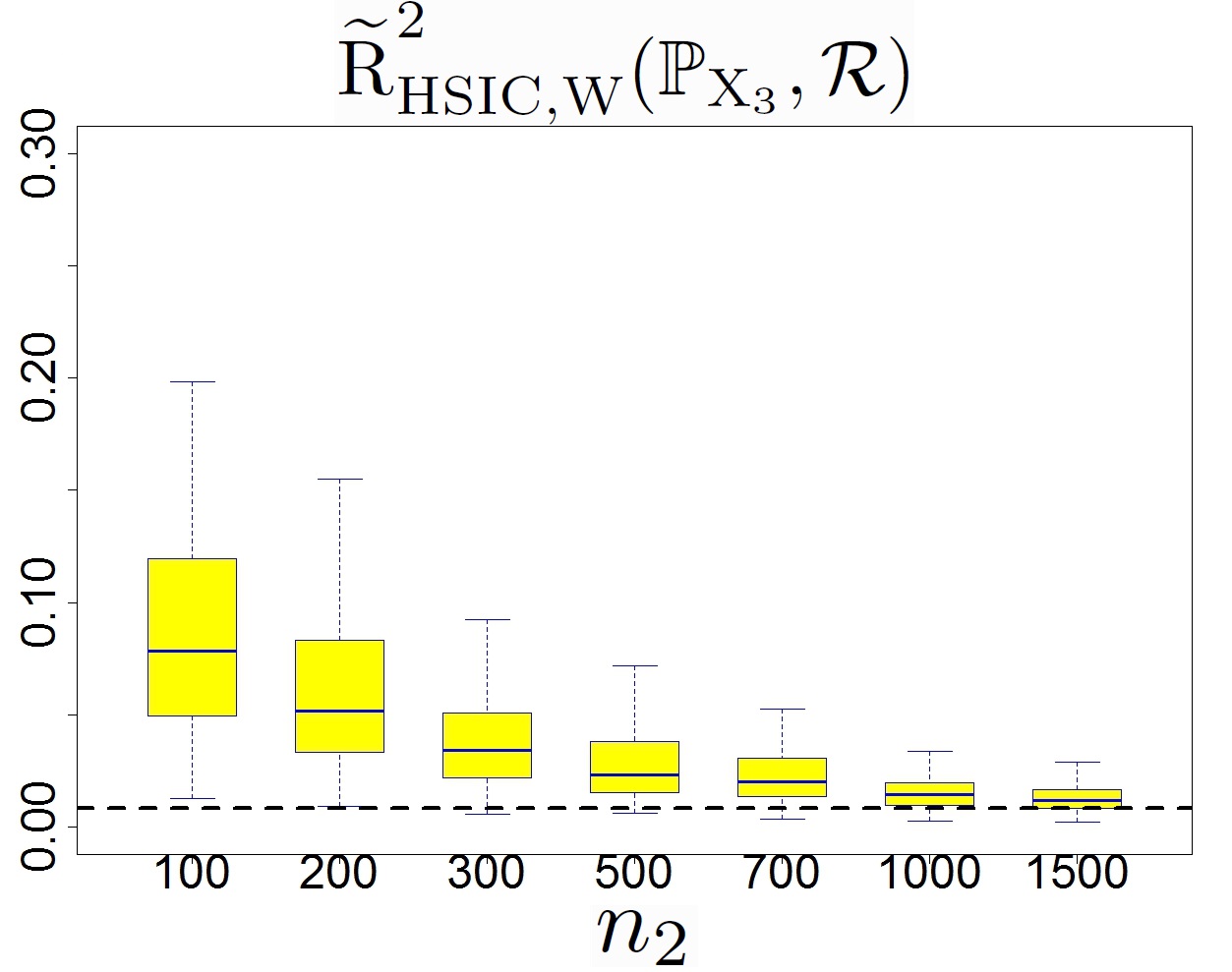
Figure 2: Convergence plots of the estimators $\widetilde{\operatorname{R}2}^{2}_{\operatorname{HSIC},\operatorname{M}}(\mathbb{P}_{X_{k}},\mathcal{R})$, $\widetilde{\operatorname{R}2}^{2}_{\operatorname{HSIC},\operatorname{W}}(\mathbb{P}_{X_{k}},\mathcal{R})$ and $\widetilde{\operatorname{R}2}^{2}_{\operatorname{HSIC},\operatorname{K}}(\mathbb{P}_{X_{k}},\mathcal{R}),k=1,\ldots,3$, for the model $h$ and w.r.t the size $n_{2}$ of samples. Theorical values are represented in dotted lines.

In addition, we compare the ability of the three estimators to correctly order $\mathbb{P}_{X_{k}},k=1\ldots 3$ by order of influence. For this, we compute for each sample size, the ratio of times when they give the good theorical ranking. Table (2) gives the good ranking rates of 2${}^{\text{nd}}$-level $\operatorname{R}2^{2}_{\operatorname{HSIC}}$ estimators w.r.t the sample size. These results confirm that the estimators based on mixture and Kullback-Leibler barycenter laws outperform those based on Wasserstein barycenter law. Both $\widetilde{\operatorname{R}2}^{2}_{\operatorname{HSIC},\operatorname{M}}(\mathbb{P}_{X_{k}},\mathcal{R})$ and $\widetilde{\operatorname{R}2}^{2}_{\operatorname{HSIC},\operatorname{K}}(\mathbb{P}_{X_{k}},\mathcal{R})$ yield highly accurate ranking from $n_{2}=500$ against $n_{2}=700$ for $\widetilde{\operatorname{R}2}^{2}_{\operatorname{HSIC},\operatorname{W}}(\mathbb{P}_{X_{k}},\mathcal{R})$. Furthermore, the Kullback-Leibler barycenter seems to give slightly better results for small samples $n_{2}\leq 300$, this being reversed from $n_{2}=500$. The lower performance of Wasserstein barycenter law could be explained by the fact that the ratio $\displaystyle\frac{f}{f_{W}}$ becomes very high in the neighborhood of 0.

$n_{2}$	$100$	$200$	$300$	$500$	$700$	$1000$	$1500$
$\widetilde{\operatorname{R}2}^{2}_{\operatorname{HSIC},\operatorname{M}}(\mathbb{P}_{X_{k}},\mathcal{R})$	$74\%$	$79\%$	$84\%$	$94.5\%$	$97\%$	$100\%$	$100\%$
$\widetilde{\operatorname{R}2}^{2}_{\operatorname{HSIC},\operatorname{K}}(\mathbb{P}_{X_{k}},\mathcal{R})$	$75.5\%$	$79\%$	$87\%$	$92\%$	$97\%$	$99.5\%$	$99.5\%$
$\widetilde{\operatorname{R}2}^{2}_{\operatorname{HSIC},\operatorname{W}}(\mathbb{P}_{X_{k}},\mathcal{R})$	$57.5\%$	$71\%$	$77\%$	$82\%$	$91\%$	$93.5\%$	$98\%$

Table 2: Good ranking rates of $\left(\mathbb{P}_{X_{i}}\right)_{i=1..3}$ given by the estimators $\widetilde{\operatorname{R}2}^{2}_{\operatorname{HSIC},\operatorname{M}}(\mathbb{P}_{X_{k}},\mathcal{R})$, $\widetilde{\operatorname{R}2}^{2}_{\operatorname{HSIC},\operatorname{K}}(\mathbb{P}_{X_{k}},\mathcal{R})$ and $\widetilde{\operatorname{R}2}^{2}_{\operatorname{HSIC},\operatorname{W}}(\mathbb{P}_{X_{k}},\mathcal{R})$ for the model $h$, w.r.t the size $n_{2}$ of samples.

4.1.3 Comparison with Monte Carlo "double loop" approach

In this part, we compare the "single loop" estimation of 2${}^{\text{nd}}$-level HSIC measures with the "double loop" estimation. For this, we consider a total budget $n=1026$ simulations for both methods and propose the following test:

• For the "double loop" approach, a sample of size $n_{2}=38$ is generated for each triplet of input distributions ($n=n_{1}\times n_{2}=1026$ simulations). The computed "double loop" estimators are denoted $\widehat{\operatorname{R}2}^{2}_{\operatorname{HSIC}}(\mathbb{P}_{X_{k}},\mathcal{R}),k=1\ldots 3$.

• For the "single loop" approach, we apply the proposed methodology with $n_{2}=1026$ to compute the "single loop" estimators $\widetilde{\operatorname{R}2}^{2}_{\operatorname{HSIC},\operatorname{M}}(\mathbb{P}_{X_{k}},\mathcal{R})$ and $\widetilde{\operatorname{R}2}^{2}_{\operatorname{HSIC},\operatorname{K}}(\mathbb{P}_{X_{k}},\mathcal{R})$, $k=1\ldots 3$.

This numerical test is repeated 200 times with independent Monte Carlo samples. Figure 3 shows the dispersion of the obtained estimators. Theoretical values are shown in dotted lines. We observe that the "double loop" estimators have much more variability than "single loop" ones (especially for the distribution $\mathbb{P}_{X_{3}}$). We even observe a much larger bias (especially for $\mathbb{P}_{X_{3}}$) for the "double loop" approach. Good ranking rates are given by Table 3 and confirm that our proposed "single loop" approach significantly outperforms the "double loop" approach.

This example illustrates the interest of the "simple loop" approach which allows a much more accurate estimation of 2${}^{\text{nd}}$-level HSIC measures. Indeed, for a given total budget of $n$ simulations, 1${}^{\text{st}}$-level HSIC are computed via modified HSIC from $n_{2}=n$ simulations in our "single loop" approach against $n_{2}=n/n_{1}$ in the "double loop" one. Even if classical estimators converge faster than modified ones, the number of simulations available for their estimation is drastically reduced with the double loop approach.

On this same analytical function, other numerical tests with different hypothesis on the input distributions (more different from each other) have been performed and yield similar results and conclusions.

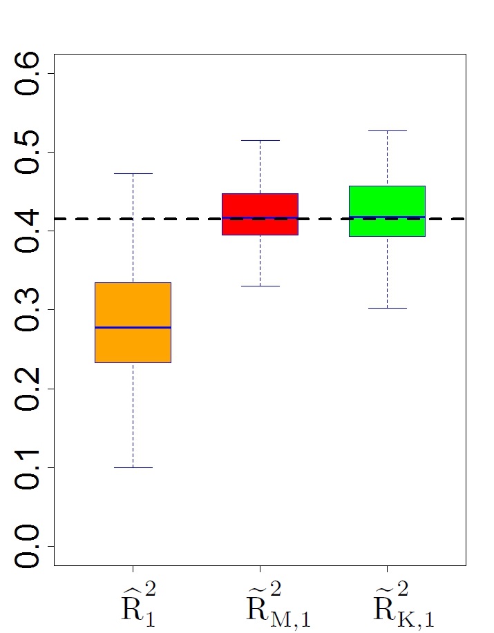
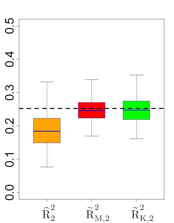
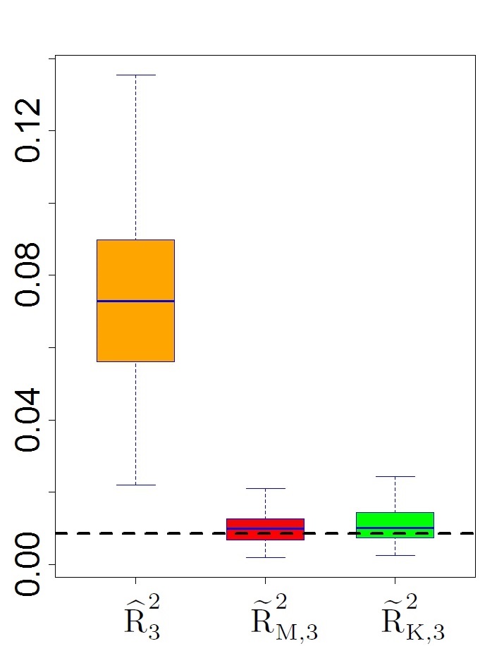
Figure 3: Comparison of convergence plots of 2${}^{\text{nd}}$-level GSA indices by "double loop" approach ($\widehat{\operatorname{R}2}^{2}_{k}=\widehat{\operatorname{R}2}^{2}_{\operatorname{HSIC}}(\mathbb{P}_{X_{k}},\mathcal{R})$) and by "single loop" approach ($\widetilde{\operatorname{R}2}^{2}_{\operatorname{M},k}=\widetilde{\operatorname{R}2}^{2}_{\operatorname{HSIC},\operatorname{M}}(\mathbb{P}_{X_{k}},\mathcal{R})$ and $\widetilde{\operatorname{R}2}^{2}_{\operatorname{K},k}=\widetilde{\operatorname{R}2}^{2}_{\operatorname{HSIC},\operatorname{K}}(\mathbb{P}_{X_{k}},\mathcal{R})$) for the model $h$ and $n=1026$. Theorical values are represented in dotted lines.

Double loop	Single loop
$\widehat{\operatorname{R}2}^{2}_{\operatorname{HSIC}}(\mathbb{P}_{X_{k}},\mathcal{R})$	$\widetilde{\operatorname{R}2}^{2}_{\operatorname{HSIC},\operatorname{M}}(\mathbb{P}_{X_{k}},\mathcal{R})$	$\widetilde{\operatorname{R}2}^{2}_{\operatorname{HSIC},\operatorname{K}}(\mathbb{P}_{X_{k}},\mathcal{R})$
$67.5\%$	$100\%$	$99\%$

Table 3: Comparison of good ranking rates of "double loop" and "simple loop" estimators, for model $h$ and $n=1026$.

4.2 Nuclear safety application

Within the framework of 4${}^{\text{th}}$-generation sodium-cooled fast reactor ASTRID: Advanced Sodium Technological Reactor for Industrial Demonstration (see Figure 4), the CEA (French Commissariat à l’Énergie atomique et aux Énergies alternatives) provides numerical tools in order to assess the safety in case of several accidents. For this, various physical modelling tools have been developed to study different severe accidental scenarios. Among these physical modelling tools, a numerical tool called MACARENa (French: Modélisation de l’ACcident d’Arrêt des pompes d’un REacteur refroidi au sodium) developped by [15] simulates a primary phase of an Unprotected Loss Of Flow (ULOF) accident. During this type of accident, the power loss of primary pumps and the dysfunction of shutdown systems cause a gradual decrease of the sodium flow in the primary circuit, which subsequently may increase the temperature of sodium until it boils. This temperature increase can lead to a degradation of several components and structures of the reactor core.

Previous GSA studies were performed on MACARENa simulator with several tens of uncertain parameters whose pdf were assumed to be known and set at a reference pdf (see [14] for more details). These studies showed the predominant influence of only 3 parameters on the accident transient predicted by MACARENa:

• $X_{1}$: error of measurement on external pressure loss,

• $X_{2}$: primary half-flow time,

• $X_{3}$: Lockart-Martinelli correction value.

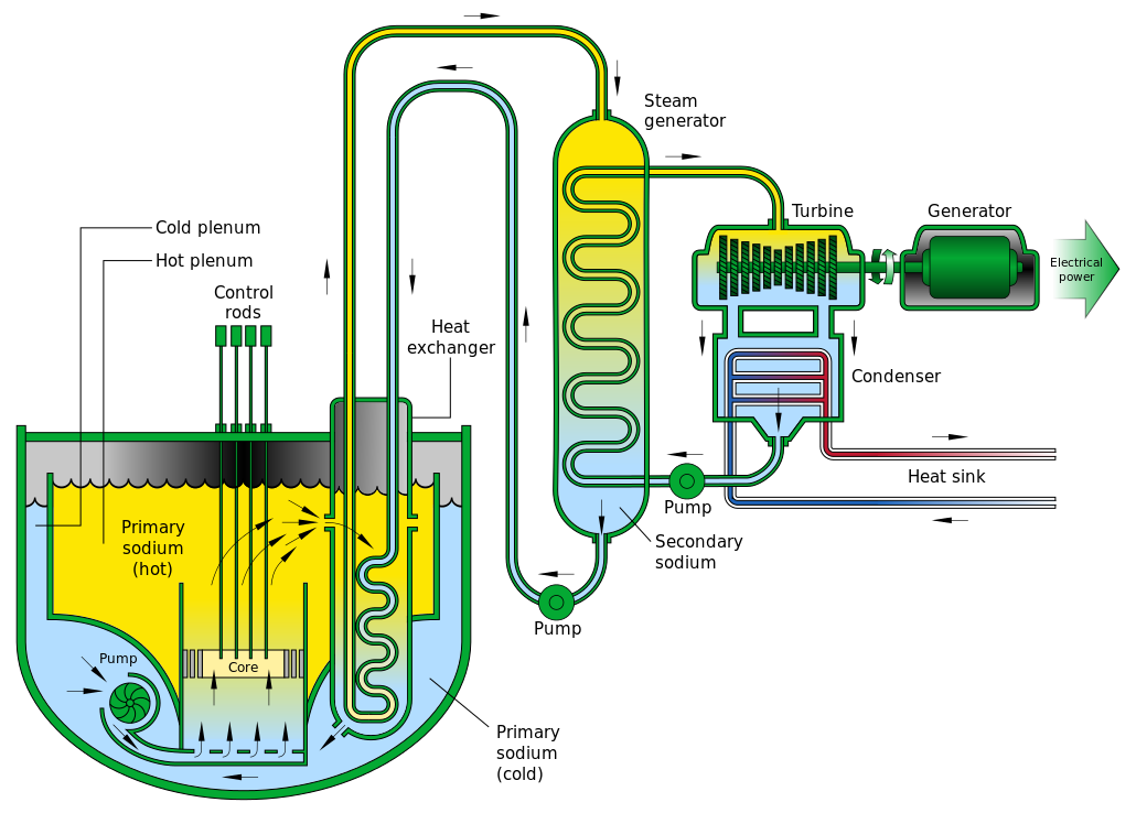
Figure 4: Basic architecture of a Sodium-cooled Fast Reactor

However, due to lack of data and knowledge, uncertainty remains on the distributions $\mathbb{P}_{X_{1}}$, $\mathbb{P}_{X_{2}}$ and $\mathbb{P}_{X_{3}}$ respectively of $X_{1}$, $X_{2}$ and $X_{3}$. To take into account this uncertainty, for each input, the type of law is assumed to be known but one of its parameters is uncertain, as described in Table (4). The notations $\mathcal{N}_{t}(a,b,m,\sigma)$, $\operatorname{T}(a,b,c)$ and $\mathcal{U}(a,b)$ are respectively, the truncated normal law of mean $m$ and standard deviation $\sigma$ on $[a,b]$, the triangular law on $[a,b]$ with mode $c$ and the uniform law on $[a,b]$.

Law of input	Nature	Uncertain parameter
$\mathbb{P}_{X_{1}}$	$\mathcal{N}_{t}(-0.1,0.1,0,\sigma)$	$\sigma\sim\mathcal{U}(0.03,0.05)$
$\mathbb{P}_{X_{2}}$	$\operatorname{T}(0,20,c)$	$c\sim\mathcal{U}(8,15)$
$\mathbb{P}_{X_{3}}$	$\operatorname{T}(0.8,2,m)$	$m\sim\mathcal{U}(1,1.5)$

Table 4: Uncertainties on the laws $\mathbb{P}_{X_{1}}$,$\mathbb{P}_{X_{2}}$ and $\mathbb{P}_{X_{3}}$.

Among the outputs computed by MACARENa simulator to describe the ULOF accident, we focus on the first instant of sodium boiling denoted $Y$. The objective is then to assess how each uncertainty on input pdf can impact the results of sensitivity analysis of $Y$.

Methodological choices. In order to perform GSA2, we apply our proposed algorithm with the following methodological choices (see Section 3.3):

• the unique sample for each input is generated according to the mixture law,

• the quantity of interest characterizing GSA1 results is the vector $\mathbf{\operatorname{R}2^{2}_{\operatorname{HSIC}}}$,

• the RKHS kernel based on the MMD distance is used for input distributions and the standardized Gaussian kernel is used for GSA1 results.

Choices of sample sizes $n_{1}$ and $n_{2}$. We consider a Monte Carlo sample of size $n_{2}=1000$ for the unique sample. This choice is motivated by two main reasons, firstly the calculation time of one simulation of MACARENa (between 2 and 3 hours on average) which limits the total number of simulations and secondly the analytical three-dimensional example of Section (4.1) for which a budget of 1000 simulations gave good results. Furthermore, for the sample of distributions, we consider a Monte Carlo sample of $n_{1}=200$ triplets of pdf. These two choices for $n_{1}$ and $n_{2}$ will then be justified later in this section, by checking the convergence of estimators.

By applying our 2${}^{\text{nd}}$ GSA methodology, with all these choices, we obtain the following 2${}^{\text{nd}}$-level sensitivity indices values:

• $\widetilde{\operatorname{R}2}^{2}_{\operatorname{HSIC},\operatorname{M}}(\mathbb{P}_{X_{1}},\mathcal{R})=0.5341$,

• $\widetilde{\operatorname{R}2}^{2}_{\operatorname{HSIC},\operatorname{M}}(\mathbb{P}_{X_{2}},\mathcal{R})=0.3317$,

• $\widetilde{\operatorname{R}2}^{2}_{\operatorname{HSIC},\operatorname{M}}(\mathbb{P}_{X_{3}},\mathcal{R})=0.0753$.

Consequently, uncertainty on $\mathbb{P}_{X_{1}}$ mainly impacts GSA1 results, followed by $\mathbb{P}_{X_{2}}$, while $\mathbb{P}_{X_{3}}$ has a negligible impact. Therefore, the efforts of characterization must be targeted on $\mathbb{P}_{X_{1}}$ to improve the confidence in GSA1 results. Note that, similar results and conclusions are obtained considering for $\mathcal{R}$ the ranking of $X_{1}$, $X_{2}$ and $X_{3}$ using 1${}^{\text{st}}$-level $\operatorname{R}2^{2}_{\operatorname{HSIC}}$.

Remark 4.2.

A deeper analysis of the 200 GSA1 results shows that $X_{2}$ is almost all the time the predominant input ($99\%$ of cases). On the other hand, the rank of $X_{3}$ or $X_{1}$ varies: $X_{3}$ is the least influential input in $63\%$ of cases, against $37\%$ for $X_{1}$.

In the light of GSA2 results, this alternation between the rank of $X_{3}$ and $X_{1}$ is therefore mainly driven by the uncertainty on $\mathbb{P}_{X_{1}}$, to a lesser extend by $\mathbb{P}_{X_{2}}$, while $\mathbb{P}_{X_{3}}$ has no impact. Moreover, $X_{2}$ whose distribution is not the most influential on GSA1 result, is surprisingly, the most influential inputs on $Y$. This example illustrates, if necessary, that GSA2 aims to capture an information that is different but complementary to that of GSA1.

In order to assess the accuracy of 2${}^{\text{nd}}$-level $\operatorname{R}2^{2}_{\operatorname{HSIC}}$ estimation, we use a non-asymptotic bootstrapping approach (see e.g. [16]). For this, we first generate Monte Carlo subsamples with replacement from the initial sample (of 1000 simulations), then we re-estimate 2${}^{\text{nd}}$-level $\operatorname{R}2^{2}_{\operatorname{HSIC}}$ using these samples. We consider in particular subsamples of sizes $n_{2}=100$ to $n_{2}=800$. For each size, the estimation is repeated independently $B=20$ times. Furthermore, to reduce computational efforts, we consider a sample of distributions of reduced size $n_{1}=30$ and generated with a space-filling approach. More precisely, the vector $(\sigma,c,m)$ is sampled with a Maximum Projection Latin Hypercube Design [29] of size $n_{1}=30$ and defined on the cubic domain $[0.03,0.05]\times[8,15]\times[1,1.5]$.

Figure (5) presents as a boxplot the mismatch between the value estimated from the initial sample and the values estimated from subsamples. We first observe a robustness of estimation: the means of estimators seem to match the value given by the initial sample. We notice also high dispersions for small and medium sizes ($n_{2}\leq 400$) and small dispersions for medium and big sizes ($n_{2}\geq 500$). Therefore, it can be deduced that the estimations of GSA2 indices with the sample of $n_{2}=1000$ simulations have converged, the stabilization of the estimations being satisfactory from $n_{2}=700$.

We also test the robustness of the estimation in terms of ranking of input distributions. Table (5) gives for each subsample size, the rate of times that the ranking matches with the ranking obtained on the initial sample. The results given by Table (5) validate the conclusions drawn from convergence plots (5).

$n_{2}=100$	$n_{2}=200$	$n_{2}=300$	$n_{2}=400$	$n_{2}=500$	$n_{2}=600$	$n_{2}\geq 700$
$45\%$	$55\%$	$70\%$	$75\%$	$95\%$	$95\%$	$100\%$

Table 5: Good ranking rates given by the estimators $\widetilde{\operatorname{R}2}^{2}_{\operatorname{HSIC},\operatorname{M}}(\mathbb{P}_{X_{k}},\mathcal{R})$ for MACARENa w.r.t the size $n_{2}$ of the unique sample.

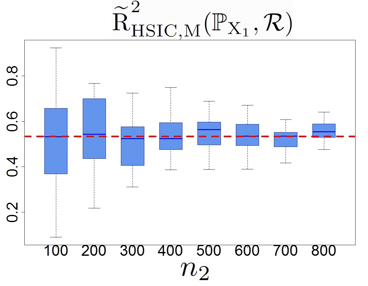
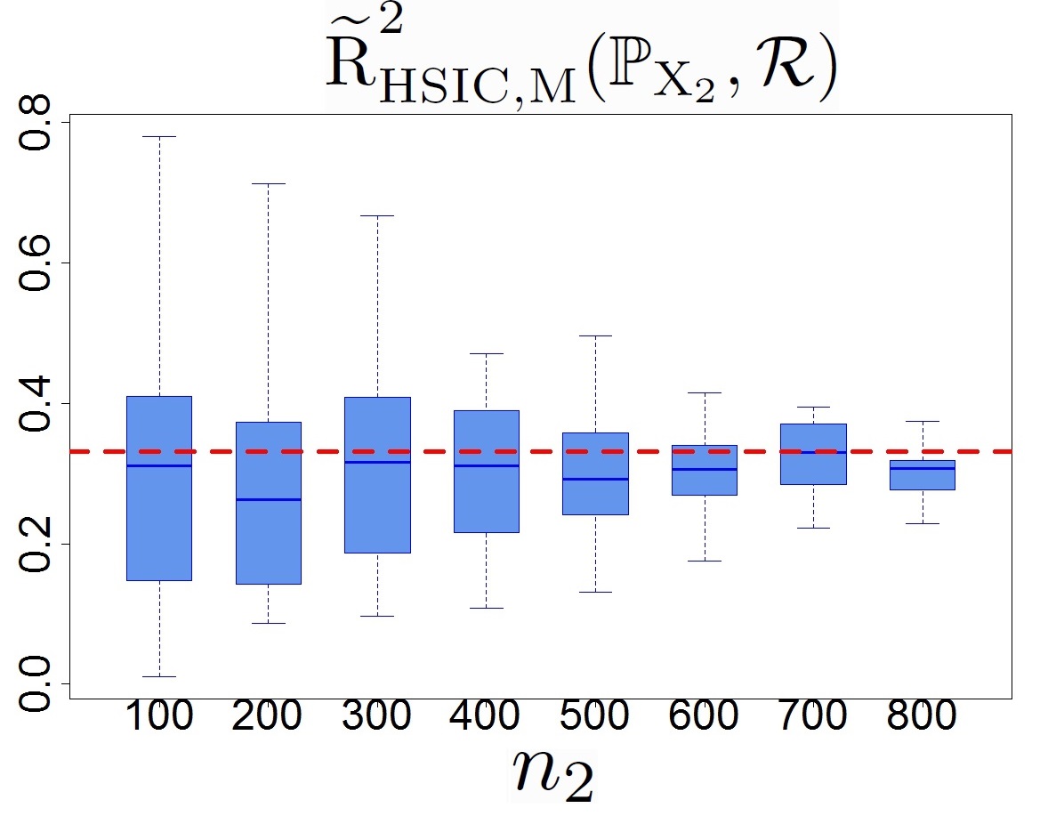
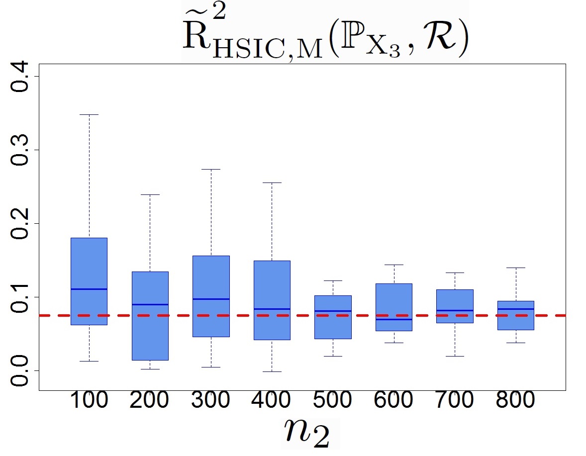
Figure 5: Convergence plots of the estimators $\widetilde{\operatorname{R}2}^{2}_{\operatorname{HSIC},\operatorname{M}}(\mathbb{P}_{X_{k}},\mathcal{R})$ for MACARENa, according to the sample size $n_{2}$. Theoretical values are represented in red dashed lines.

5 Conclusion and Prospect

In this article, we proposed a new methodology for second-level Global Sensitivity Analysis (GSA2) based on Hilbert-Schmidt Independence Criterion (HSIC). For this, we first proposed new weighted estimators for HSIC, using an alternative sample generated according to a probability distribution which is not the prior distribution of the inputs. We also demonstrated the properties of these new estimators (bias, variance and asymptotic law), which are similar to those of classical estimators. Moreover, their convergence has been illustrated on an analytical example which has also highlighted their ability to correctly rank variables (even for small and medium sample sizes). Subsequently, 2${}^{\text{nd}}$-level GSA based on HSIC measures is discussed. When input distributions are uncertain, GSA2 purpose is to assess the impact of these uncertainties on GSA results. In order to perform GSA2, we presented a new "single loop" Monte Carlo methodology to address problems raised by GSA2: characterization of GSA results, definition of 2${}^{\text{nd}}$-level HSIC measures and limitation of the calculation budget. This methodology is based on a single sample generated according to a "reference distribution" (related to the set of all possible distributions). Three options have been proposed for this distribution: mixture law and barycentric laws w.r.t symmetrized Kullback-Leibler distance or Wasserstein distance. The estimation of 2${}^{\text{nd}}$-level HSIC seems to be more accurate using the two first options rather than the Wasserstein barycenter. We also illustrated the great interest of the "single loop" approach compared to the "double loop" approach. Finally, the whole methodology has been applied to a nuclear test case simulating a severe reactor accident and has shown how GSA2 can provide additional information to classical GSA.

Several points of the methodology could be more investigated in future research. First, we could focus on comparing Space Filling Design (see e.g. [34], [8], [46]) techniques and Monte Carlo methods for the sampling of input distribution in the case of probabilistic densities (pdf) with uncertain parameters. Indeed, sampling the uncertain parameters of pdf following a space-filling design could improve the accuracy of the estimators of GSA2 indices. Another interesting perspective would be to build independence tests based on 2${}^{\text{nd}}$-level HSIC measures estimators. This could be achieved by identifying the asymptotic distributions of these estimators under the assumption of independence between distributions and GSA1 results.

Furthermore, this new approach for GSA2 could also be compared to the classical approach of epistemic GSA in the framework of Dempster-Shafer theory (see [37], [2]). Indeed, Dempster-Shafer theory gives a description of random variables with epistemic uncertainty, which is to associate with an epistemic variable $Z$ on a set $A$, a mass function representing a probability measure on the set $\mathcal{P}(A)$ of all $A$-subsets. This lack of knowledge is reflected in Dempster-Shafer theory by an upper and lower bound of the cumulative distribution function and can be viewed as 2${}^{\text{nd}}$-level of uncertainty.

An other potential prospect could be to make the connection between our approach and Perturbed-Law based Indices (PLI) [30]. These indices are used to quantify the impact of a perturbation of an input density on the failure probability (probability that a model output exceeds a given threshold). To compare our GSA2 indices with PLI, the probability of failure could be considered as the quantity of interest characterizing GSA results in our methodology. Last but not least, GSA2 method can be compared to the approach proposed in [6] which models 2${}^{\text{nd}}$-level uncertainties as a uni-level uncertainty on the vector $(\Theta,X)$, where $\Theta$ is the vector of uncertain parameters.

Proofs

B Proof of Proposition 1

In this annex, we prove that:

$$\widetilde{\operatorname{HSIC}}(X_{k},Y)=\displaystyle\frac{1}{n^{2}}\operatorname{Tr}\left(\operatorname{W}\operatorname{\widetilde{L}}_{k}\operatorname{W}H_{1}\operatorname{\widetilde{L}}\operatorname{H_{2}}\right).$$

Firstly, we evaluate the matrix $\operatorname{W}\operatorname{\widetilde{L}}_{k}\operatorname{W}H_{1}\operatorname{\widetilde{L}}\operatorname{H_{2}}$ coefficients before computing its trace. The matrix $\operatorname{W}$ being diagonal, we write for $i,j\in\{1,\ldots,n\}$:

$$(\operatorname{W}\operatorname{\widetilde{L}}_{k}\operatorname{W})_{i,j}=(\operatorname{\widetilde{L}}_{k})_{i,j}\operatorname{W}_{i,i}\operatorname{W}_{j,j}.$$

The coefficient of the matrix $\operatorname{W}\operatorname{\widetilde{L}}_{k}\operatorname{W}H_{1}$ indexed by $i$ and $j$ can therefore be computed:

$$(\operatorname{W}\operatorname{\widetilde{L}}_{k}\operatorname{W}H_{1})_{i,j} =\displaystyle\sum_{r=1}^{n}(\operatorname{\widetilde{L}}_{k})_{i,r}\operatorname{W}_{i,i}\operatorname{W}_{r,r}(H_{1})_{r,j}$$

$$=\displaystyle\sum_{r=1}^{n}(\operatorname{\widetilde{L}}_{k})_{i,r}\operatorname{W}_{i,i}\operatorname{W}_{r,r}(\delta_{r,j}-\displaystyle\frac{1}{n}\operatorname{W}_{j,j})$$

$$=(\operatorname{\widetilde{L}}_{k})_{i,j}\operatorname{W}_{i,i}\operatorname{W}_{j,j}-\displaystyle\frac{1}{n}\sum_{r=1}^{n}(\operatorname{\widetilde{L}}_{k})_{i,r}\operatorname{W}_{i,i}\operatorname{W}_{r,r}\operatorname{W}_{j,j}.$$

Subsequently, the matrix $\operatorname{W}\operatorname{\widetilde{L}}_{k}\operatorname{W}H_{1}\operatorname{\widetilde{L}}$ coefficients are obtained:

$$(\operatorname{W}\operatorname{\widetilde{L}}_{k}\operatorname{W}H_{1}\operatorname{\widetilde{L}})_{i,j} =\displaystyle\sum_{r=1}^{n}(\operatorname{W}\operatorname{\widetilde{L}}_{k}\operatorname{W}H_{1})_{i,r}\operatorname{\widetilde{L}}_{r,j}$$

$$=\displaystyle\sum_{r=1}^{n}\left((\operatorname{\widetilde{L}}_{k})_{i,r}\operatorname{W}_{i,i}\operatorname{W}_{r,r}-\displaystyle\frac{1}{n}\sum_{s=1}^{n}(\operatorname{\widetilde{L}}_{k})_{i,s}\operatorname{W}_{i,i}\operatorname{W}_{s,s}\operatorname{W}_{r,r}\right)\operatorname{\widetilde{L}}_{r,j}$$

$$=\displaystyle\sum_{r=1}^{n}(\operatorname{\widetilde{L}}_{k})_{i,r}\operatorname{\widetilde{L}}_{r,j}\operatorname{W}_{i,i}\operatorname{W}_{r,r}-\displaystyle\frac{1}{n}\sum_{s=1}^{n}(\operatorname{\widetilde{L}}_{k})_{i,s}\operatorname{W}_{i,i}\operatorname{W}_{s,s}\sum_{r=1}^{n}\operatorname{\widetilde{L}}_{r,j}\operatorname{W}_{r,r}.$$

Finally,

$$(\operatorname{W}\operatorname{\widetilde{L}}_{k}\operatorname{W}H_{1}\operatorname{\widetilde{L}}\operatorname{H_{2}})_{i,j} =\displaystyle\sum_{r=1}^{n}(\operatorname{W}\operatorname{\widetilde{L}}_{k}\operatorname{W}H_{1}\operatorname{\widetilde{L}})_{i,r}(\operatorname{H_{2}})_{r,j}$$

$$=\displaystyle\sum_{r=1}^{n}(\operatorname{W}\operatorname{\widetilde{L}}_{k}\operatorname{W}H_{1}\operatorname{\widetilde{L}})_{i,r}(\delta_{r,j}-\displaystyle\frac{1}{n}\operatorname{W}_{r,r})$$

$$=(\operatorname{W}\operatorname{\widetilde{L}}_{k}\operatorname{W}H_{1}\operatorname{\widetilde{L}})_{i,j}-\displaystyle\frac{1}{n}\displaystyle\sum_{r=1}^{n}(\operatorname{W}\operatorname{\widetilde{L}}_{k}\operatorname{W}H_{1}\operatorname{\widetilde{L}})_{i,r}\operatorname{W}_{r,r}$$

$$=\displaystyle\sum_{r=1}^{n}(\operatorname{\widetilde{L}}_{k})_{i,r}\operatorname{\widetilde{L}}_{r,j}\operatorname{W}_{i,i}\operatorname{W}_{r,r}-\displaystyle\frac{1}{n}\sum_{1\leq r,s\leq n}(\operatorname{\widetilde{L}}_{k})_{i,s}\operatorname{\widetilde{L}}_{r,j}\operatorname{W}_{i,i}\operatorname{W}_{s,s}\operatorname{W}_{r,r}$$

$$-\displaystyle\frac{1}{n}\sum_{r=1}^{n}\left(\displaystyle\sum_{s=1}^{n}(\operatorname{\widetilde{L}}_{k})_{i,s}\operatorname{\widetilde{L}}_{s,r}\operatorname{W}_{i,i}\operatorname{W}_{s,s}-\displaystyle\frac{1}{n}\sum_{1\leq p,q\leq n}(\operatorname{\widetilde{L}}_{k})_{i,q}\operatorname{\widetilde{L}}_{p,r}\operatorname{W}_{i,i}\operatorname{W}_{q,q}\operatorname{W}_{p,p}\right)\operatorname{W}_{r,r}$$

$$=\displaystyle\sum_{r=1}^{n}(\operatorname{\widetilde{L}}_{k})_{i,r}\operatorname{\widetilde{L}}_{r,j}\operatorname{W}_{i,i}\operatorname{W}_{r,r}-\displaystyle\frac{1}{n}\sum_{1\leq r,s\leq n}(\operatorname{\widetilde{L}}_{k})_{i,s}\operatorname{\widetilde{L}}_{r,j}\operatorname{W}_{i,i}\operatorname{W}_{s,s}\operatorname{W}_{r,r}$$

$$-\displaystyle\frac{1}{n}\sum_{1\leq r,s\leq n}(\operatorname{\widetilde{L}}_{k})_{i,s}\operatorname{\widetilde{L}}_{s,r}\operatorname{W}_{i,i}\operatorname{W}_{s,s}\operatorname{W}_{r,r}+\displaystyle\frac{1}{n^{2}}\sum_{1\leq r,p,q\leq n}(\operatorname{\widetilde{L}}_{k})_{i,q}\operatorname{\widetilde{L}}_{p,r}\operatorname{W}_{i,i}\operatorname{W}_{q,q}\operatorname{W}_{p,p}\operatorname{W}_{r,r}.$$

Summing up the matrix $\operatorname{W}\operatorname{\widetilde{L}}_{k}\operatorname{W}H_{1}\operatorname{\widetilde{L}}\operatorname{H_{2}}$ diagonal terms, then dividing by $n^{2}$ gives:

$$\displaystyle\frac{1}{n^{2}}\operatorname{Tr}\left(\operatorname{W}\operatorname{\widetilde{L}}_{k}\operatorname{W}H_{1}\operatorname{\widetilde{L}}\operatorname{H_{2}}\right) =\displaystyle\frac{1}{n^{2}}\sum_{1\leq i,r\leq n}(\operatorname{\widetilde{L}}_{k})_{i,r}\operatorname{\widetilde{L}}_{i,r}\operatorname{W}_{i,i}\operatorname{W}_{r,r}+\displaystyle\frac{1}{n^{4}}\sum_{1\leq i,q\leq n}(\operatorname{\widetilde{L}}_{k})_{i,q}\operatorname{W}_{i,i}\operatorname{W}_{q,q}\sum_{1\leq p,r\leq n}\operatorname{\widetilde{L}}_{p,r}\operatorname{W}_{p,p}\operatorname{W}_{r,r}$$

$$-\displaystyle\frac{2}{n^{3}}\sum_{1\leq i,r,s\leq n}(\operatorname{\widetilde{L}}_{k})_{i,s}\operatorname{\widetilde{L}}_{i,r}\operatorname{W}_{i,i}\operatorname{W}_{s,s}\operatorname{W}_{r,r}.$$

By definition of $\operatorname{\widetilde{L}}_{k}$, $\operatorname{\widetilde{L}}$ and $\operatorname{W}$, the three terms of the last equation are respectively the estimators defined in Formula (12).

C Proof of Proposition 2

Throughout the rest of the document, to lighten formulas, we denote $(l_{k})_{i,j}=(\operatorname{\widetilde{L}}_{k})_{i,j}$ , $l_{i,j}=\operatorname{\widetilde{L}}_{i,j}$ and $\operatorname{w}_{i}=\operatorname{W}_{i,i}$. We also denote $\operatorname{\widetilde{HSIC}_{U}}(X_{k},Y)$ the U-statistic associated to the estimator $\widetilde{\operatorname{HSIC}}(X_{k},Y)$.

Under the null hypothesis $\mathcal{H}_{0,k}$, the estimator $\operatorname{\widetilde{HSIC}_{U}}(X_{k},Y)$ is unbiased. The estimator $\widetilde{\operatorname{HSIC}}(X_{k},Y)$ bias, is then equal to that of $\widetilde{\operatorname{HSIC}}(X_{k},Y)-\operatorname{\widetilde{HSIC}_{U}}(X_{k},Y)$ under this same assumption. We first compute the expression of $\widetilde{\operatorname{HSIC}}(X_{k},Y)-\operatorname{\widetilde{HSIC}_{U}}(X_{k},Y)$, before computing its expectation. We recall that,

$$\widetilde{\operatorname{HSIC}}(X_{k},Y) ={} \displaystyle\frac{1}{n^{2}}\sum_{1\leq i,j\leq n}(l_{k})_{i,j}l_{i,j}\operatorname{w}_{i}\operatorname{w}_{j}+\displaystyle\frac{1}{n^{4}}\sum_{1\leq i,j,p,q\leq n}(l_{k})_{i,j}l_{p,q}\operatorname{w}_{i}\operatorname{w}_{j}\operatorname{w}_{p}\operatorname{w}_{q}$$

$$-{} \displaystyle\frac{2}{n^{3}}\sum_{1\leq i,j,r\leq n}(l_{k})_{i,j}l_{i,r}\operatorname{w}_{i}\operatorname{w}_{j}\operatorname{w}_{r}$$

$$:= \operatorname{\widetilde{H}^{1}_{k}}1k+\operatorname{\widetilde{H}^{2}_{k}}-2\operatorname{\widetilde{H}^{3}_{k}},$$

$$\operatorname{\widetilde{HSIC}_{U}}(X_{k},Y) ={} \displaystyle\frac{1}{(n)_{2}}\sum_{(i,j)\in i^{n}_{2}}(l_{k})_{i,j}l_{i,j}\operatorname{w}_{i}\operatorname{w}_{j}+\displaystyle\frac{1}{(n)_{4}}\sum_{(i,j,p,q)\in i^{n}_{4}}(l_{k})_{i,j}l_{p,q}\operatorname{w}_{i}\operatorname{w}_{j}\operatorname{w}_{p}\operatorname{w}_{q}$$

$$-{} \displaystyle\frac{2}{(n)_{3}}\sum_{(i,j,r)\in i^{n}_{3}}(l_{k})_{i,j}l_{i,r}\operatorname{w}_{i}\operatorname{w}_{j}\operatorname{w}_{r}$$

$$:={} \operatorname{\widetilde{H}^{1,U}_{k}}1k+\operatorname{\widetilde{H}^{2,U}_{k}}-2\operatorname{\widetilde{H}^{3,U}_{k}},$$

where $(n)_{s}=\displaystyle\frac{n!}{(n-s)!}$ and $i^{n}_{s}$ is the set of all s-tuples drawn without replacement from the set $\{1,\ldots,n\}$.

Let us compute $\widetilde{\operatorname{HSIC}}(X_{k},Y)-\operatorname{\widetilde{HSIC}_{U}}(X_{k},Y)$ term by term:

$$\operatorname{\widetilde{H}^{1}_{k}}1k-\operatorname{\widetilde{H}^{1,U}_{k}}1k ={} \displaystyle\frac{1}{n^{2}}\displaystyle\sum_{i=1}^{n}(l_{k})_{i,i}l_{i,i}\operatorname{w}_{i}^{2}-\displaystyle\frac{1}{n^{2}(n-1)}\displaystyle\sum_{1\leq i\neq j\leq n}(l_{k})_{i,j}l_{i,j}\operatorname{w}_{i}\operatorname{w}_{j},$$

$$\operatorname{\widetilde{H}^{2}_{k}}-\operatorname{\widetilde{H}^{2,U}_{k}} ={} \displaystyle\frac{1}{n^{4}}\sum_{(i,j,q)\in i_{3}^{n}}\left[(l_{k})_{i,i}l_{j,q}\operatorname{w}_{i}^{2}\operatorname{w}_{j}\operatorname{w}_{q}+4(l_{k})_{i,j}l_{i,q}\operatorname{w}_{i}^{2}\operatorname{w}_{j}\operatorname{w}_{q}+(l_{k})_{i,j}l_{q,q}\operatorname{w}_{i}\operatorname{w}_{j}\operatorname{w}_{q}^{2}\right]$$

$$-{} \displaystyle\frac{6}{n(n)_{4}}\sum_{(i,j,p,q)\in i_{4}^{n}}(l_{k})_{i,j}l_{p,q}\operatorname{w}_{i}\operatorname{w}_{j}\operatorname{w}_{p}\operatorname{w}_{q}+O(\frac{1}{n^{2}}),$$

$$\operatorname{\widetilde{H}^{3}_{k}}-\operatorname{\widetilde{H}^{3,U}_{k}} ={} \displaystyle\frac{1}{n^{3}}\sum_{1\leq i\neq j\leq n}\left[(l_{k})_{i,i}l_{i,j}\operatorname{w}_{i}^{2}\operatorname{w}_{j}+(l_{k})_{i,j}l_{i,i}\operatorname{w}_{i}^{2}\operatorname{w}_{j}+(l_{k})_{i,j}l_{i,j}\operatorname{w}_{i}\operatorname{w}_{j}^{2}\right]$$

$$-{} \displaystyle\frac{3}{n(n)_{3}}\displaystyle\sum_{(i,j,r)\in i_{3}^{n}}(l_{k})_{i,j}l_{i,r}\operatorname{w}_{i}\operatorname{w}_{j}\operatorname{w}_{r}+O(\frac{1}{n^{2}}).$$

These expressions can be simplified by replacing $(l_{k})_{i,i}=l_{i,i}=1$:

$$\operatorname{\widetilde{H}^{1}_{k}}1k-\operatorname{\widetilde{H}^{1,U}_{k}}1k =\displaystyle\frac{1}{n^{2}}\displaystyle\sum_{i=1}^{n}\operatorname{w}_{i}^{2}-\displaystyle\frac{1}{n^{2}(n-1)}\displaystyle\sum_{1\leq i\neq j\leq n}(l_{k})_{i,j}l_{i,j}\operatorname{w}_{i}\operatorname{w}_{j},$$

$$\operatorname{\widetilde{H}^{2}_{k}}-\operatorname{\widetilde{H}^{2,U}_{k}} =\displaystyle\frac{1}{n^{4}}\sum_{(i,j,q)\in i_{3}^{n}}\left[l_{j,q}\operatorname{w}_{i}^{2}\operatorname{w}_{j}\operatorname{w}_{q}+4(l_{k})_{i,j}l_{i,q}\operatorname{w}_{i}^{2}\operatorname{w}_{j}\operatorname{w}_{q}+(l_{k})_{i,j}\operatorname{w}_{i}\operatorname{w}_{j}\operatorname{w}_{q}^{2}\right]$$

$$-\displaystyle\frac{6}{n(n)_{4}}\sum_{(i,j,p,q)\in i_{4}^{n}}(l_{k})_{i,j}l_{p,q}\operatorname{w}_{i}\operatorname{w}_{j}\operatorname{w}_{p}\operatorname{w}_{q}+O(\frac{1}{n^{2}}),$$

$$\operatorname{\widetilde{H}^{3}_{k}}-\operatorname{\widetilde{H}^{3,U}_{k}} =\displaystyle\frac{1}{n^{3}}\sum_{1\leq i\neq j\leq n}\left[l_{i,j}\operatorname{w}_{i}^{2}\operatorname{w}_{j}+(l_{k})_{i,j}\operatorname{w}_{i}^{2}\operatorname{w}_{j}+(l_{k})_{i,j}l_{i,j}\operatorname{w}_{i}\operatorname{w}_{j}^{2}\right]$$

$$-\displaystyle\frac{3}{n(n)_{3}}\displaystyle\sum_{(i,j,r)\in i_{3}^{n}}(l_{k})_{i,j}l_{i,r}\operatorname{w}_{i}\operatorname{w}_{j}\operatorname{w}_{r}+O(\frac{1}{n^{2}}).$$

By computing the expectation of these three estimators under $\mathcal{H}_{0,k}$, we have:

$$\mathbb{E}\left[\operatorname{\widetilde{H}^{1}_{k}}1k-\operatorname{\widetilde{H}^{1,U}_{k}}1k\right] =\displaystyle\frac{1}{n}\left(\operatorname{E}_{\omega}-\operatorname{E}_{x_{k}}\operatorname{E}_{y}\right),$$

$$\mathbb{E}\left[\operatorname{\widetilde{H}^{2}_{k}}-\operatorname{\widetilde{H}^{2,U}_{k}}\right] =\displaystyle\frac{1}{n}\left(\operatorname{E}_{\omega}\operatorname{E}_{y}+4\operatorname{E}_{x_{k},\omega}\operatorname{E}_{y,\omega}+\operatorname{E}_{\omega}\operatorname{E}_{x_{k}}\right)-\displaystyle\frac{6}{n}\;\operatorname{E}_{x_{k}}\operatorname{E}_{y}+O(\frac{1}{n^{2}}),$$

$$\mathbb{E}\left[\operatorname{\widetilde{H}^{3}_{k}}-\operatorname{\widetilde{H}^{3,U}_{k}}\right] =\displaystyle\frac{1}{n}\left(\operatorname{E}_{\omega}^{k}\operatorname{E}_{y,\omega}+\operatorname{E}_{\omega}^{-k}\operatorname{E}_{x_{k},\omega}+\operatorname{E}_{x_{k},\omega}\operatorname{E}_{y,\omega}\right)-\displaystyle\frac{3}{n}\operatorname{E}_{x_{k}}\operatorname{E}_{y}+O(\frac{1}{n^{2}}).$$

From these last equations, we obtain:

$$\mathbb{E}\left[\widetilde{\operatorname{HSIC}}(X_{k},Y)-\operatorname{\widetilde{HSIC}_{U}}(X_{k},Y)\right] =\displaystyle\frac{2}{n}(\operatorname{E}_{\omega}^{k}-\operatorname{E}_{x_{k},\omega})(\operatorname{E}_{\omega}^{-k}-\operatorname{E}_{y,\omega})-\displaystyle\frac{1}{n}(\operatorname{E}_{\omega}-\operatorname{E}_{x_{k}})(\operatorname{E}_{\omega}-\operatorname{E}_{y})$$

$$+\displaystyle\frac{1}{n}\operatorname{E}_{\omega}(\operatorname{E}_{\omega}-1)+O(\displaystyle\frac{1}{n^{2}}).$$

Finally, The bias of $\widetilde{\operatorname{HSIC}}(X_{k},Y)$ under $\mathcal{H}_{0,k}$ is written:

$$\mathbb{E}[\widetilde{\operatorname{HSIC}}(X_{k},Y)]-\operatorname{HSIC}(X_{k},Y) =\displaystyle\frac{2}{n}(\operatorname{E}_{\omega}^{k}-\operatorname{E}_{x_{k},\omega})(\operatorname{E}_{\omega}^{-k}-\operatorname{E}_{y,\omega})-\displaystyle\frac{1}{n}(\operatorname{E}_{\omega}-\operatorname{E}_{x_{k}})(\operatorname{E}_{\omega}-\operatorname{E}_{y})$$

$$+\displaystyle\frac{1}{n}\operatorname{E}_{\omega}(\operatorname{E}_{\omega}-1)+O(\displaystyle\frac{1}{n^{2}}).$$

D Proof of Proposition 3

In order to compute the variance of $\widetilde{\operatorname{HSIC}}(X_{k},Y)$ and to determine its asymptotic law under $\mathcal{H}_{0,k}$, general theorems on V-statistics must be used. For this, we write this last estimator as a single V-statistic. By analogy with theorem 1 of [23], we have:

$$\widetilde{\operatorname{HSIC}}(X_{k},Y)=\displaystyle\frac{1}{n^{4}}\sum_{1\leq i,j,q,r\leq n}\widetilde{\operatorname{h}}_{ijqr},$$

where

$$\widetilde{\operatorname{h}}_{i,j,q,r}=\displaystyle\frac{1}{4!}\sum_{(t,u,v,s)}^{(i,j,q,r)}(l_{k})_{t,u}l_{t,u}\operatorname{w}_{t}\operatorname{w}_{u}+(l_{k})_{t,u}l_{v,s}\operatorname{w}_{t}\operatorname{w}_{u}\operatorname{w}_{v}\operatorname{w}_{s}-2(l_{k})_{t,u}l_{t,v}\operatorname{w}_{t}\operatorname{w}_{u}\operatorname{w}_{v},$$

the sum represents all ordered quadruples $(t,u,v,s)$ drawn without replacement from $(i,j,q,r)$.

This equality is easily obtained by decomposing the last sum into three sums, then by writing that:

$$\begin{array}[]{ll}\displaystyle\frac{1}{n^{4}}\sum_{1\leq i,j,q,r\leq n}\frac{1}{4!}\sum_{(t,u,v,s)}^{(i,j,q,r)}(l_{k})_{t,u}l_{t,u}\operatorname{w}_{t}\operatorname{w}_{u}&=\displaystyle\frac{1}{n^{2}}\sum_{1\leq i,j\leq n}(l_{k})_{i,j}l_{i,j}\operatorname{w}_{i}\operatorname{w}_{j},\\ \\ \displaystyle\frac{1}{n^{4}}\sum_{1\leq i,j,q,r\leq n}\frac{1}{4!}\sum_{(t,u,v,s)}^{(i,j,q,r)}(l_{k})_{t,u}l_{v,s}\operatorname{w}_{t}\operatorname{w}_{u}\operatorname{w}_{v}\operatorname{w}_{s}&=\displaystyle\frac{1}{n^{4}}\sum_{1\leq i,j,q,r\leq n}(l_{k})_{i,j}l_{q,r}\operatorname{w}_{i}\operatorname{w}_{j}\operatorname{w}_{q}\operatorname{w}_{r},\\ \\ \displaystyle\frac{1}{n^{4}}\sum_{1\leq i,j,q,r\leq n}\frac{1}{4!}\sum_{(t,u,v,s)}^{(i,j,q,r)}(l_{k})_{t,u}l_{t,v}\operatorname{w}_{t}\operatorname{w}_{u}\operatorname{w}_{v}&=\displaystyle\frac{1}{n^{3}}\sum_{1\leq i,j,r\leq n}(l_{k})_{i,j}l_{i,r}\operatorname{w}_{i}\operatorname{w}_{j}\operatorname{w}_{r}.\end{array}$$

The result is then obtained by combining the last three equalities.

Remark .1.

The U-statistic associated to the estimator $\widetilde{\operatorname{HSIC}}(X_{k},Y)$ is written:

$$\operatorname{\widetilde{HSIC}_{U}}(X_{k},Y)=\displaystyle\frac{1}{(n)_{4}}\sum_{(i,j,q,r)\in i_{4}^{n}}\widetilde{\operatorname{h}}_{ijqr}.$$

Under $\mathcal{H}_{0,k}$, the estimators $n\times\widetilde{\operatorname{HSIC}}(X_{k},Y)$ et $n\times\operatorname{\widetilde{HSIC}_{U}}(X_{k},Y)$ have the same asymptotic behavior (see e.g. [36]). Moreover, Hoeffding variance decomposition of $\operatorname{\widetilde{HSIC}_{U}}(X_{k},Y)$ is written:

$$\operatorname{Var}\left(\operatorname{\widetilde{HSIC}_{U}}(X_{k},Y)\right)={n\choose 4}^{-1}\displaystyle\sum_{r=1}^{4}{r\choose 4}{n-4\choose 4-r}\zeta_{r},$$

where $\zeta_{r}=\operatorname{Var}\left(\mathbb{E}[\widetilde{h}_{i,j,p,q}\mid X_{1},\ldots,X_{r}]\right),r=1,\ldots,4$.

Moreover, under $\mathcal{H}_{0,k}$, the variance of $\operatorname{\widetilde{HSIC}_{U}}(X_{k},Y)$ converges to $0$ in $\displaystyle O(\frac{1}{n^{2}})$:

$$\operatorname{Var}(\operatorname{\widetilde{HSIC}_{U}}(X_{k},Y))=\displaystyle\frac{72(n-4)(n-5)}{n(n-1)(n-2)(n-3)}\zeta_{2}+O(\frac{1}{n^{3}}).$$

Under $\mathcal{H}_{0,k}$, $\zeta_{2}=\mathbb{E}_{i,j}\left[\mathbb{E}_{q,r}[\widetilde{h}_{i,j,p,q}]^{2}\right]$, where the notation $\mathbb{E}_{r,s}$ designates the expectation by integrating only w.r.t variables $X_{r}$ and $X_{s}$.

Moreover, by detailing the different terms of $\widetilde{h}_{i,j,p,q}$, we easily show that:

$$6\widetilde{h}_{ijqr} =(l_{k})_{i,j}\operatorname{w}_{i}\operatorname{w}_{j}\left(l_{i,j}+l_{q,r}\operatorname{w}_{q}\operatorname{w}_{r}\right)+(l_{k})_{i,q}\operatorname{w}_{i}\operatorname{w}_{q}\left(l_{i,q}+l_{j,r}\operatorname{w}_{j}\operatorname{w}_{r}\right)+(l_{k})_{i,r}\operatorname{w}_{i}\operatorname{w}_{r}\left(l_{i,r}+l_{j,q}\operatorname{w}_{j}\operatorname{w}_{q}\right)$$

$$+(l_{k})_{j,q}\operatorname{w}_{j}\operatorname{w}_{q}\left(l_{j,q}+l_{i,r}\operatorname{w}_{i}\operatorname{w}_{r}\right)+(l_{k})_{j,r}\operatorname{w}_{j}\operatorname{w}_{r}\left(l_{j,r}+l_{q,i}\operatorname{w}_{q}\operatorname{w}_{i}\right)+(l_{k})_{q,r}\operatorname{w}_{q}\operatorname{w}_{r}\left(l_{q,r}+l_{i,j}\operatorname{w}_{i}\operatorname{w}_{j}\right)$$

$$-\displaystyle\frac{1}{2}\sum_{(t,u,v)}^{(i,j,q,r)}(l_{k})_{t,u}\operatorname{w}_{t}\operatorname{w}_{u}\left(l_{t,v}\operatorname{w}_{v}+l_{u,v}\operatorname{w}_{v}\right)$$

where

$$(l_{k})_{i,.} =\widetilde{\mathbb{E}}\left[\operatorname{\widetilde{L}}_{k}\left(X_{k}^{(i)},X_{k}\right)\omega_{k}(X_{k})\right], l_{i,.} =\widetilde{\mathbb{E}}\left[\operatorname{\widetilde{L}}\left(Y^{(i)},Y\right)\omega_{-k}(X_{-k})\right],$$

$$(l_{k})_{.,j} =\widetilde{\mathbb{E}}\left[\operatorname{\widetilde{L}}_{k}\left(X_{k}^{(j)},X_{k}\right)\omega_{k}(X_{k})\right], l_{j,.} =\widetilde{\mathbb{E}}\left[\operatorname{\widetilde{L}}\left(Y^{(j)},Y\right)\omega_{-k}(X_{-k})\right],$$

$$(l_{k}) =\widetilde{\mathbb{E}}\left[\operatorname{\widetilde{L}}_{k}\left(X^{\prime}_{k},X_{k}\right)\omega_{k}(X_{k})\right], l =\widetilde{\mathbb{E}}\left[\operatorname{\widetilde{L}}\left(Y^{\prime},Y\right)\omega_{-k}(X_{-k})\right].$$

We therefore write under $\mathcal{H}_{0,k}$:

$$6E_{q,r}\left[\widetilde{h}_{ijqr}\right] =(\widetilde{l}_{k})_{i,j}\operatorname{w}_{i}\operatorname{w}_{j}\left(\widetilde{l}_{i,j}-\widetilde{l}_{i,.}-\widetilde{l}_{j,.}+\widetilde{l}\right)-(\widetilde{l}_{k})_{i,.}\operatorname{w}_{i}\left(l_{i,j}\operatorname{w}_{j}-l_{i,.}-l_{j,.}\operatorname{w}_{j}+l\right)$$

$$-(l_{k})_{.,j}\operatorname{w}_{j}\left(l_{i,j}\operatorname{w}_{i}-l_{i,.}\operatorname{w}_{i}-l_{j,.}+l\right)-(l_{k})\left(l_{i,j}\operatorname{w}_{i}\operatorname{w}_{j}-l_{i,.}\operatorname{w}_{i}-l_{j,.}\operatorname{w}_{j}+l\right).$$

$E_{q,r}\left[\widetilde{h}_{ijqr}\right]$ can be estimated empirically by $\displaystyle\frac{1}{6}(\widetilde{B})_{i,j}$, where $\widetilde{B}$ is the matrice defined in Formula (16). The variance $\zeta_{2}$ can be estimated by: $\widehat{\zeta_{2}}=\displaystyle\frac{1}{36n^{2}}\mathbf{1}^{T}(\widetilde{B}\odot\widetilde{B})\mathbf{1}$. Formula (16) is then obtained by replacing the expression of $\widehat{\zeta_{2}}$, in Hoeffding’s decomposition.

E Proof of Theorem 1

The asymptotic law of the V-statistic $n\times\widetilde{\operatorname{HSIC}}(X_{k},Y)$ (as well as the U-statistic $n\times\operatorname{\widetilde{HSIC}_{U}}(X_{k},Y)$) is given by Theorem 5.5.2, page 194 of [36], which gives a formulation of the asymptotic laws of degenerate V-statistics (and U-statistics). Indeed, under $\mathcal{H}_{0,k}$ the statistic $\widetilde{\operatorname{HSIC}}(X_{k},Y)$ is degenerate, that is: $\forall(i,j,q,r)\in\{1,..,n\}:\mathbb{E}\left[\widetilde{h}_{ijqr}\right]=0$.

Theorem.

Under $\mathcal{H}_{0,k}$ we have the following two law convergence theorems:

$$n\times\widetilde{\operatorname{HSIC}}^{V}(\widetilde{X}_{k},\widetilde{Y})\; \overset{\mathcal{L}}{\longrightarrow}\displaystyle\sum_{l=1}^{+\infty}\;\lambda_{l}\widetilde{z}_{l}^{2},$$

$$n\times\widetilde{\operatorname{HSIC}}^{U}(\widetilde{X}_{k},\widetilde{Y})\; \overset{\mathcal{L}}{\longrightarrow}\displaystyle\sum_{l=1}^{+\infty}\;\lambda_{l}\left(\widetilde{z}_{l}^{2}-1\right)$$

where $\left(\widetilde{z}_{l}\right)_{l\geq 1}$ are independent and identically distributed random variables of law $\mathcal{N}(0,1)$ and $\left(\lambda_{l}\right)_{l\geq 1}$ are the eigenvalues of the following operator:

$$A(g):z\mapsto\displaystyle\int\widetilde{h}_{ijqr}(\widetilde{z},\widetilde{z}_{j},\widetilde{z}_{q},\widetilde{z}_{r})\;g(\widetilde{z}_{j})\;dF_{jqr}$$

where $dF_{jqr}$ denotes random variables $\widetilde{z}_{j}$, $\widetilde{z}_{q}$ and $\widetilde{z}_{r}$.

To conclude, the distribution $\displaystyle\sum_{l=1}^{+\infty}\;\lambda_{l}\widetilde{z}_{l}^{2}$ can be approximated by a Gamma law according to [23]. In fact, it is an infinite sum of random variables independent of law $\chi^{2}$ (Chi two). The asymptotic law of the V-statistic $n\times\widetilde{\operatorname{HSIC}}(X_{k},Y)$ under $\mathcal{H}_{0,k}$ is a Gamma law, whose parameters can be estimated based on the empirical expectation and variance of $n\times\widetilde{\operatorname{HSIC}}(X_{k},Y)$ (see section 2.2.2).

References

• [1] Martial Agueh and Guillaume Carlier. Barycenters in the wasserstein space. SIAM Journal on Mathematical Analysis, 43(2):904–924, 2011.
• [2] Diego A Alvarez. Reduction of uncertainty using sensitivity analysis methods for infinite random sets of indexable type. International journal of approximate reasoning, 50(5):750–762, 2009.
• [3] Nachman Aronszajn. Theory of reproducing kernels. Matematika, 7(2):67–130, 1963.
• [4] Charles R Baker. Joint measures and cross-covariance operators. Transactions of the American Mathematical Society, 186:273–289, 1973.
• [5] Claire Cannaméla. Apport des méthodes probabilistes dans la simulation du comportement sous irradiation du combustible à particules. PhD thesis, Paris 7, 2007.
• [6] Vincent Chabridon, Mathieu Balesdent, Jean-Marc Bourinet, Jérôme Morio, and Nicolas Gayton. Evaluation of failure probability under parameter epistemic uncertainty: application to aerospace system reliability assessment. Aerospace Science and Technology, 69:526–537, 2017.
• [7] Andreas Christmann and Ingo Steinwart. Universal kernels on non-standard input spaces. In Advances in neural information processing systems, pages 406–414, 2010.
• [8] Thomas M Cioppa. Efficient nearly orthogonal and space-filling experimental designs for high-dimensional complex models. PhD thesis, 2002.
• [9] Imre Csiszár. A class of measures of informativity of observation channels. Periodica Mathematica Hungarica, 2(1-4):191–213, 1972.
• [10] Sebastien Da Veiga. Global sensitivity analysis with dependence measures. Journal of Statistical Computation and Simulation, 85(7):1283–1305, 2015.
• [11] Guillaume Damblin, Mathieu Couplet, and Bertrand Iooss. Numerical studies of space-filling designs: optimization of latin hypercube samples and subprojection properties. Journal of Simulation, 7(4):276–289, 2013.
• [12] Matthias De Lozzo and Amandine Marrel. New improvements in the use of dependence measures for sensitivity analysis and screening. Journal of Statistical Computation and Simulation, 86(15):3038–3058, 2016.
• [13] Etienne De Rocquigny, Nicolas Devictor, and Stefano Tarantola. Uncertainty in industrial practice. Wiley, 2008.
• [14] Jean-Baptiste Droin. Modélisation d’un transitoire de perte de débit primaire non protégé dans un RNR-Na. PhD thesis, Université Grenoble Alpes, 2016.
• [15] Jean-Baptiste Droin, Nathalie Marie, Andrea Bachrata, Frederic Bertrand, Elsa Merle, and Jean-Marie Seiler. Physical tool for unprotected loss of flow transient simulations in a sodium fast reactor. Annals of nuclear energy, 106:195–210, 2017.
• [16] Bradley Efron and Robert J Tibshirani. An introduction to the bootstrap. CRC press, 1994.
• [17] B. Everitt and D.J. Hand. Finite Mixture Distributions. Monographs on applied probability and statistics. Chapman and Hall, 1981.
• [18] Kenji Fukumizu, Francis R Bach, and Michael I Jordan. Dimensionality reduction for supervised learning with reproducing kernel hilbert spaces. Journal of Machine Learning Research, 5(Jan):73–99, 2004.
• [19] Kenji Fukumizu, Arthur Gretton, Xiaohai Sun, and Bernhard Schölkopf. Kernel measures of conditional dependence. In Advances in neural information processing systems, pages 489–496, 2008.
• [20] Clark R Givens, Rae Michael Shortt, et al. A class of wasserstein metrics for probability distributions. The Michigan Mathematical Journal, 31(2):231–240, 1984.
• [21] Arthur Gretton, Karsten M Borgwardt, Malte J Rasch, Bernhard Schölkopf, and Alexander Smola. A kernel two-sample test. Journal of Machine Learning Research, 13:723–773, 2012.
• [22] Arthur Gretton, Olivier Bousquet, Alex Smola, and Bernhard Scholkopf. Measuring statistical dependence with hilbert-schmidt norms. In International conference on algorithmic learning theory, volume 16, pages 63–78. Springer, 2005.
• [23] Arthur Gretton, Kenji Fukumizu, Choon H Teo, Le Song, Bernhard Schölkopf, and Alex J Smola. A kernel statistical test of independence. In Advances in neural information processing systems, pages 585–592, 2008.
• [24] J.C. Helton, J.D. Johnson, C.J. Sallaberry, and C.B. Storlie. Survey of sampling-based methods for uncertainty and sensitivity analysis. Reliability Engineering & System Safety, 91(10-11):1175 – 1209, 2006.
• [25] Bertrand Iooss and Paul Lemaître. A review on global sensitivity analysis methods. In Uncertainty management in simulation-optimization of complex systems, pages 101–122. Springer, 2015.
• [26] T Ishigami and Toshimitsu Homma. An importance quantification technique in uncertainty analysis for computer models. In Uncertainty Modeling and Analysis, 1990. Proceedings., First International Symposium on, pages 398–403. IEEE, 1990.
• [27] Yunlong Jiao and Jean-Philippe Vert. The kendall and mallows kernels for permutations. IEEE transactions on pattern analysis and machine intelligence, 40(7):1755–1769, 2018.
• [28] Don Johnson and Sinan Sinanovic. Symmetrizing the kullback-leibler distance. IEEE Transactions on Information Theory, 2001.
• [29] V Roshan Joseph, Evren Gul, and Shan Ba. Maximum projection designs for computer experiments. Biometrika, 102(2):371–380, 2015.
• [30] Paul Lemaître, Ekatarina Sergienko, Aurélie Arnaud, Nicolas Bousquet, Fabrice Gamboa, and Bertrand Iooss. Density modification-based reliability sensitivity analysis. Journal of Statistical Computation and Simulation, 85(6):1200–1223, 2015.
• [31] Horia Mania, Aaditya Ramdas, Martin J Wainwright, Michael I Jordan, Benjamin Recht, et al. On kernel methods for covariates that are rankings. Electronic Journal of Statistics, 12(2):2537–2577, 2018.
• [32] Charles A Micchelli, Yuesheng Xu, and Haizhang Zhang. Universal kernels. Journal of Machine Learning Research, 7(Dec):2651–2667, 2006.
• [33] R v Mises. On the asymptotic distribution of differentiable statistical functions. The annals of mathematical statistics, 18(3):309–348, 1947.
• [34] Luc Pronzato and Werner G Müller. Design of computer experiments: space filling and beyond. Statistics and Computing, 22(3):681–701, 2012.
• [35] Andrea Saltelli, Marco Ratto, Terry Andres, Francesca Campolongo, Jessica Cariboni, Debora Gatelli, Michaela Saisana, and Stefano Tarantola. Global sensitivity analysis: the primer. John Wiley & Sons, 2008.
• [36] Robert J Serfling. Approximation theorems of mathematical statistics, volume 162. John Wiley & Sons, 2009.
• [37] Philippe Smets. What is dempster-shafer’s model. Advances in the Dempster-Shafer theory of evidence, pages 5–34, 1994.
• [38] Ilya M Sobol. Sensitivity estimates for nonlinear mathematical models. Mathematical Modelling and Computational Experiments, 1(4):407–414, 1993.
• [39] Bharath K Sriperumbudur, Arthur Gretton, Kenji Fukumizu, Bernhard Schölkopf, and Gert RG Lanckriet. Hilbert space embeddings and metrics on probability measures. Journal of Machine Learning Research, 11:1517–1561, 2010.
• [40] Ingo Steinwart. On the influence of the kernel on the consistency of support vector machines. Journal of machine learning research, 2(Nov):67–93, 2001.
• [41] Zoltán Szabó and Bharath K Sriperumbudur. Characteristic and universal tensor product kernels. Journal of Machine Learning Research, 18(233):1–29, 2018.
• [42] Gábor J Székely, Maria L Rizzo, Nail K Bakirov, et al. Measuring and testing dependence by correlation of distances. The annals of statistics, 35(6):2769–2794, 2007.
• [43] D Michael Titterington, Adrian FM Smith, and Udi E Makov. Statistical analysis of finite mixture distributions. Wiley,, 1985.
• [44] Raymond Veldhuis. The centroid of the symmetrical kullback-leibler distance. IEEE signal processing letters, 9(3):96–99, 2002.
• [45] Cédric Villani. Topics in optimal transportation. Number 58. American Mathematical Soc., 2003.
• [46] G Gary Wang and Songqing Shan. Review of metamodeling techniques in support of engineering design optimization. Journal of Mechanical design, 129(4):370–380, 2007.