Machine Learning Non-Markovian Quantum Dynamics

Abstract

Machine learning methods have proved to be useful for the recognition of patterns in statistical data. The measurement outcomes are intrinsically random in quantum physics, however, they do have a pattern when the measurements are performed successively on an open quantum system. This pattern is due to the system-environment interaction and contains information about the relaxation rates as well as non-Markovian memory effects. Here we develop a method to extract the information about the unknown environment from a series of projective single-shot measurements on the system (without resorting to the process tomography). The method is based on embedding the non-Markovian system dynamics into a Markovian dynamics of the system and the effective reservoir of finite dimension. The generator of Markovian embedding is learned by the maximum likelihood estimation. We verify the method by comparing its prediction with an exactly solvable non-Markovian dynamics. The developed algorithm to learn unknown quantum environments enables one to efficiently control and manipulate quantum systems.

Introduction.—

Quantum systems are never perfectly isolated which makes the study of open quantum dynamics important for various disciplines including solid-state physics takahashi-2008 , quantum chemistry valkunas-2013 , quantum sensing degen-2017 , quantum information transmission wilde-2017 , and quantum computing nielsen-2000 . Open quantum dynamics is a result of interaction between the system of interest and its environment. It is usually assumed that the environment is an infinitely large reservoir in statistical equilibrium, which has a well-defined interaction with the system schoeller-2018 . However, the environments of many physical systems are rather complex and structured piilo-2011 ; cirac-2011 ; ma-2012 ; hoope-2012 ; yang-2013 ; hughes-2015 ; eisert-2015 ; cirac-2017 ; wittemer-2018 ; wang-2018 ; peng-2018 ; haase-2018 ; mascherpa-2019 . A model of the system-environment interaction is often heuristic and oversimplified (e.g., a harmonic environment), but even in this case the analysis is rater complicated and requires some elaborated analytical and numerical methods strathearn-2018 ; pollock-2019 ; altaisky-2017 . A theoretical model may also neglect some additional sources of decoherence and relaxation. The experimental analysis of the environmental degrees of freedom is difficult because of their inaccessibility in practice. In fact, one can only get some information about the actual environment by probing the system paris-2018 ; bennink-2019 . Therefore, one faces an important problem to learn the unknown environment and its interaction with the quantum system by probing and affecting the system only.

This problem can be partly solved within the assumption of fast bath relaxation, when the system density operator $\varrho_{S}$ experiences the semigroup dynamics $\varrho_{S}(t)=e^{{\cal L}_{S}t}\varrho_{S}(0)$ with the Gorini-Kossakowski-Sudarshan-Lindblad (GKSL) generator ${\cal L}_{S}$ gks-1976 ; lindblad-1976 . In this case, the generator is reconstructed by performing a process tomography of the channel $\Phi_{S}(t_{1})=e^{{\cal L}_{S}t_{1}}$ for a fixed time $t_{1}>0$ Tomography ; howard-2006 . The actual dynamics does not usually reduce to a semigroup though de-vega-2017 ; li-2018 ; fc-2018 . The problem of learning the environment is mostly attributed to memory effects accompanying the non-Markovian dynamics. In this case, one can still resort to the process tomography of channels $\Phi_{S}(t_{1})$, $\Phi_{S}(t_{2})$, $\ldots$, $\Phi_{S}(t_{K})$ by preparing various initial system states $\varrho_{S}(0)$ and performing different measurements on the system at time moments $t_{1}<t_{2}<\ldots<t_{K}$. This procedure is time consuming because one has to gather enough statistics for all time moments (the total number of required measurements is $Kd_{S}^{8}/\epsilon^{2}$ for a $d_{S}$-dimensional quantum system and the accuracy $\epsilon$ of statistical reconstruction bogdanov-2013 ; haah-2017 ). Moreover, the tomographic reconstruction of each channel $\Phi_{S}(t_{i})$ implies resetting the environment in the same initial state after each measurement, which is difficult to control in the experiment especially for a strong coupling between the system and environment.

Recently proposed methods exploit the transfer tensor techniques Cerrilo-2014 ; TTM ; TTMTomography to learn the Nakajima-Zwanzig equation nakajima-1958 ; zwanzig-1960 $\frac{d}{dt}\varrho_{S}(t)=\int_{0}^{t}{\cal K}(t-t^{\prime})\varrho_{S}(t^{\prime})dt^{\prime}$ and the recurrent neural networks RNN for defining Lindblad operators and learning the convolutionless master equation $\frac{d}{dt}\varrho_{S}(t)={\cal L}_{S}(t)\varrho_{S}(t)$. An implementation of the latter approach in practice encounters the same difficulties related with the necessity to perform state tomography at different time steps.

In this Letter, we develop a method to learn the effective Markovian embedding MarkovEmb ; xue-2015 ; xue-2017 ; campbell-2018 ; bennink-2019 ; luchnikov-2019 for non-Markovian processes instead of learning the master equation for the system ($S$). Within such an approach, the environment is effectively divided into two parts: the first one carries memory of the system and is responsible for non-Markovian dynamics [effective reservoir ($ER$)]; the second one is memoryless and causes Markovian decoherence and dissipation of $S+ER$. The system evolution reads

$$\varrho_{S}(t) = {\rm tr}_{ER}[\varrho_{S+ER}(t)],$$ (1)

$$\frac{d\varrho_{S+ER}(t)}{dt} = {\cal L}_{S+ER}[\varrho_{S+ER}(t)],$$ (2)

where the generator ${\cal L}_{S+ER}$ governs dissipative and decoherence processes on the system and the effective reservoir.

A division of the environment into two parts is similar to the pseudomode method imamoglu-1994 ; garraway-1997 ; mazzola-2009 , the reaction coordinate model iles-smith-2014 ; iles-smith-2016 , and the non-Markovian core model tamascelli-2018 , where one derives a Markovian master equation in the GKSL form for the extended system comprising the system and a finite number of auxiliary modes. In spin-bosonic models, the Markovian embedding is justified if the bath correlation function has exponentially damped correlations mascherpa-2019 . However, for power-law bath correlation functions with long-range tails polyakov-2019 the number of auxiliary modes diverges, which limits applicability of the Markovian embedding at a long timescale.

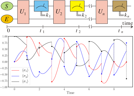
Figure 1: (Top) Interventions into the open dynamics of the system $S$ by projective measurements. Blocks $\{U_{i}\}$ depict the interaction between $S$ and the actual environment ($E$) in between the measurements. (Bottom) Example of the Bloch vector evolution for a qubit system subjected to measurements in random bases at time moments $t_{i}=i$. Circles correspond to the wave function collapse.

The density operator $\varrho_{S}(t)$ is unaccessible in a single measurement though, so any relevant information about the system is only gained in a series of measurements. On the other hand, measurement interventions into the system evolution complicate the analysis due to the no-information-without-disturbance principle. Consider a series of projective measurements performed on the system at different times $t_{1}<t_{2}<\ldots<t_{n}$, with the measurement basis being chosen randomly, see Fig. 1. The measurement outcomes seem to be completely uninformative due to the intrinsic probabilistic nature of quantum mechanics and the wave function collapse at each measurement as an example in Fig. 1 suggests. However, such a series of measurement outcomes does contain some information because the outcomes at each time moment are not equiprobable but appear in accordance with the Born rule. In this Letter, we demonstrate that a sufficiently long series of measurement results has a pattern that can be recognized by a machine carleo-2019 . This is a sharp distinction from conventional tomographic approaches based on numerous repetitions of identical experiments to gather enough statistics.

Our algorithm maximizes the likelihood of observed measurement outcomes and provides the generator ${\cal L}_{S+ER}$ for any fixed dimension of the effective reservoir $d_{ER}$, which is a hyperparameter. Computationally, the optimal $d_{ER}$ corresponds to the maximal likelihood on the validation set, which prevents overfitting supplemental . Physically, the sufficient value of $d_{ER}$ can be estimated through a reduced set of parameters: the system-environment coupling strength, the reservoir correlation time, the cutoff frequency of the spectral function, and the system’s number of degrees of freedom interacting with the environment luchnikov-2019 ; supplemental . Alternatively, $d_{ER}$ can also be estimated via the ensemble learning method shrapnel-2018 .

If the system evolution is Markovian ($d_{ER}=1$), then the result of measurement at time $t_{k}$ depends on the measurement outcome at time $t_{k-1}$ only and does not depend on results of earlier measurements at times $t_{k-2},t_{k-3},\ldots$ lindblad-1979 . Instead, the non-Markovian dynamics is accompanied by correlations in the measurement outcomes lindblad-1979 ; pollock-2018 ; modi-2018 ; budini-2018 ; taranto-2019 , which can be analyzed via the process matrix costa-2016 and the process tensor milz-2017 . The process tensor is a particular form of a quantum network chiribella-2009 , which is defined through the generator ${\cal L}_{S+ER}$ in our model, see Fig. 2. The reconstruction of a general process tensor requires exponentially many projective measurements milz-2018 . However, the process tensor has a peculiar form in our model and depends on the generator ${\cal L}_{S+ER}$ only, so it can be reconstructed by maximizing the likelihood of getting the observed outcomes for a single series of measurements without resorting to the full quantum tomography.

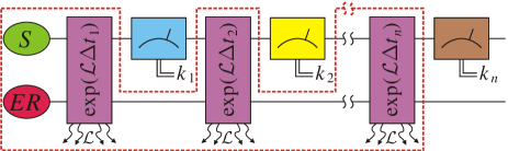
Figure 2: Markovian embedding of the open dynamics: $S$ and effective reservoir $ER$ experience semigroup dynamics with the generator ${\cal L}$; $\Delta t_{i}=t_{i}-t_{i-1}$. The process tensor is depicted by the dotted line.

Likelihood function and its gradient.—

Suppose the experimental setup allows for projective measurements of the system at times $t_{i}=i\tau$, $i=1,\ldots,n$, with the measurement basis $\{|\varphi_{k}^{(i)}\rangle\}_{k=1}^{d_{S}}$ being randomly chosen at each time moment $t_{i}$. Observation of the particular measurement outcome $k_{i}$ transforms the system state into $|\varphi_{k_{i}}^{(i)}\rangle\langle\varphi_{k_{i}}^{(i)}|$. Denote $E_{i}=|\varphi_{k_{i}}^{(i)}\rangle\langle\varphi_{k_{i}}^{(i)}|\otimes I_{ER}$ the projector acting on the system and effective reservoir. The collection of projectors $\{E_{i}\}_{i=1}^{n}$ is the training dataset that feeds the learning algorithm.

A superoperator $\Phi=\exp\left(\tau{\cal L}_{S+ER}\right)$ governs the system and the effective reservoir evolution in between two sequential measurements. The probability to get the particular sequence of measurement outcomes $\{k_{i}\}_{i=1}^{n}$ (the data $\{E_{i}\}_{i=1}^{n}$) equals luchnikov-2017

$$p={\rm tr}\left\{E_{n}\ldots\Phi\big{[}E_{1}\Phi[\varrho_{S+ER}(0)]E_{1}\big{]}\ldots E_{n}\right\}.$$ (3)

The likelihood (3) admits alternative useful forms. Let $\Phi^{{\dagger}}$ be dual to $\Phi$ comment , then one can split Eq. (3) after $m$th measurement and get $p={\rm tr}\big{[}\widetilde{\varrho}_{S+ER}(t_{m}){\cal E}_{S+ER}(t_{m})\big{]}$, where the recurrence relation $\widetilde{\varrho}_{S+ER}(t_{i+1})=E_{i}\Phi[\widetilde{\varrho}_{S+ER}(t_{i})]E_{i}$ with $\widetilde{\varrho}_{S+ER}(0)=\varrho_{S+ER}(0)$ defines the forward propagation of the subnormalized density operator along the tensor network in Fig. 3(a) and the recurrence relation ${\cal E}_{S+ER}(t_{i-1})=\Phi^{{\dagger}}[E_{i}{\cal E}_{S+ER}(t_{i})E_{i}]$ with ${\cal E}_{S+ER}(t_{n})=I_{S+ER}$ defines the backward propagation molmer-2013 of effects in the Heisenberg picture along the tensor network in Fig. 3(b). This leads to a “sandwich” formula

$$p={\rm tr}\big{\{}\Phi[\widetilde{\varrho}_{S+ER}(t_{m-1})]E_{m}{\cal E}_{S+ER}(t_{m})E_{m}\big{\}},$$ (4)

which is valid for all $m=1,\ldots,n$, see Fig. 3(c).

Figure 3: (a) Forward propagation for subnormalized density operators $\widetilde{\varrho}_{S+ER}(t_{i})$. (b) Backward propagation for effects ${\cal E}_{S+ER}(t_{i})$. (c) Likelihood functional in Eq. (4) and the Stinespring dilation (5) for $\Phi$ (dotted line).

The likelihood function is to be maximized over parameters of the generator ${\cal L}_{S+ER}$ defining $\Phi=\exp(\tau{\cal L}_{S+ER})$. Such a maximization is the most common approach in supervised machine learning Bishop . The problem is that not every generator ${\cal L}_{S+ER}$ defines a legitimate (completely positive and trace preserving) map $\Phi$. To overcome this obstacle and simplify the implementation of the gradient ascent method CVX , we use the Stinespring dilation for the channel $\Phi$ [see, e.g., Holevo and Fig. 3(c)]:

$$\Phi[\varrho_{S+ER}]={\rm tr}_{A}\left[U(H)\,\varrho_{S+ER}\otimes\varrho_{A}\,U^{{\dagger}}(H)\right],$$ (5)

where $\varrho_{A}$ is a fixed pure state of the $d_{A}$-dimensional ancilla ($A$), $d_{A}=(d_{S}d_{ER})^{2}$, $U(H)=\exp(-iH\tau)$ is a unitary evolution operator, and $H$ is the effective Hamiltonian of $S+ER+A$. Eq. (5) guarantees $\Phi$ is completely positive and trace preserving provided $H$ is Hermitian. The ancillary operator $\varrho_{A}$ plays the role of a renewable subenvironment in quantum collision models rau-1963 ; scarani-2002 ; filippov-2017 and memoryless (Markovian) part of the environment shrapnel-2018 .

Because of the Stinespring dilation, the likelihood function is now to be maximized over parameters of the effective Hamiltonian, i.e., matrix elements $H_{\mu\nu}=\langle\mu|H|\nu\rangle$ of $H$ in some computational basis $\{|\mu\rangle\}_{\mu=1}^{d_{S}d_{ER}d_{A}}$. This means that parameters $H_{\mu\nu}$ are iteratively adjusted in the direction of the gradient of the logarithmic likelihood $g_{\mu\nu}=\frac{\partial\log p}{\partial H_{\mu\nu}}$. Since the likelihood function is the $n$-degree monomial with respect to both operators $U(H)$ and $U^{{\dagger}}(H)$, we readily get supplemental

$$\!\!\!\!\!\!\!\!\!\!g_{\mu\nu}=\frac{1}{p}\sum_{m=1}^{n}{\rm tr}\bigg{\{}[E_{m}\,{\cal E}_{S+ER}(t_{m})\,E_{m}]\otimes I_{A}$$

$$\!\!\!\!\!\!\!\!\!\!\times\bigg{[}\frac{\partial U(H)}{\partial H_{\mu\nu}}\,\,\widetilde{\varrho}_{S+ER}(t_{m-1})\otimes\varrho_{A}\,\,U^{{\dagger}}(H)+{\rm H.c.}\bigg{]}\bigg{\}},\quad$$ (6)

where the derivative $\frac{\partial U(H)}{\partial H_{\mu\nu}}$ is expressed through the spectral decomposition $H=\sum_{k}\lambda_{k}|\psi_{k}\rangle\langle\psi_{k}|$ as supplemental

$$\frac{\partial U(H)}{\partial H_{\mu\nu}}=\sum_{k,l}\frac{e^{-i\lambda_{k}\tau}-e^{-i\lambda_{l}\tau}}{\lambda_{k}-\lambda_{l}}\langle\psi_{k}|\mu\rangle\langle\nu|\psi_{l}\rangle\,|\psi_{k}\rangle\langle\psi_{l}|.$$ (7)

Keeping in a computer memory the operators $\widetilde{\varrho}_{S+ER}(t_{i})$ and ${\cal E}_{S+ER}(t_{i})$ for forward and backward propagations, respectively, we efficiently calculate the gradient in $O(n)$ steps. Since $\log p$ is a highly nonlinear and nonconvex function with respect to parameters $H_{\mu\nu}$, its optimization is accompanied with overcoming the convergence to local extremums and the slow convergence rate. In what follows, we use techniques that were shown to perform well in such nonconvex optimization problems as neural network learning jain-2017 .

Learning algorithm.—

The learning algorithm, which estimates the generator ${\cal L}_{S+ER}$ based on the training dataset $\{E_{i}\}_{i=1}^{n}$, is as follows grigoriev_github :

1. Fix the hyperparameter $d_{ER}$. Initialize the model by randomly choosing the factorized state $\varrho_{S+ER}(0)=\varrho_{S}(0)\otimes\varrho_{ER}(0)$ and the factorized Hamiltonian $H=H_{S+ER}\otimes I_{A}$.

2. Calculate the forward-propagation operators $\{\widetilde{\varrho}_{S+ER}(t_{i})\}_{i=1}^{n}$ and the backward-propagation operators $\{{\cal E}_{S+ER}(t_{i})\}_{i=0}^{n-1}$.

3. Calculate the likelihood (4).

4. Find the spectral decomposition of the $d_{S}d_{ER}d_{A}$-dimensional operator $H$ and calculate $\frac{\partial U(H)}{\partial H_{\mu\nu}}$ via (7).

5. Estimate the gradient (Likelihood function and its gradient.—) via a batch of summands and results of items 2, 3, 4.

6. Feed the estimated gradient to an advanced optimization method [e.g., the adaptive moment estimation (Adam) algorithm Adam ] and get the increment $\Delta H$.

7. Update the Hamiltonian $H\rightarrow H+\Delta H$ and repeat items 2–6 until the likelihood converges.

8. Make use of the final update of $H$ to find the channel $\Phi$ and the generator ${\cal L}_{S+ER}=\frac{1}{\tau}\ln\Phi$.

Synthetic data generation.—

We apply the learning algorithm above to the in silico training set $\{E_{i}\}_{i=1}^{n}$ generated in a non-Markovian composite bipartite collision model lorenzo-2017 . We consider a bipartite system $S+S_{1}$ composed of the very open qubit system under study $S$ and one auxiliary qubit system $S_{1}$. The bipartite system successively interacts with identical subenvironments during some collision time supplemental . Such a model is quite rich and describes, e.g., a qubit subject to random telegraph noise. The benefit of this model is that the measurement interventions into the system evolution are explicitly taken into account supplemental .

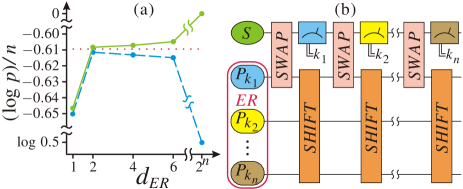
Figure 4: (a) Logarithmic likelihood per measurement vs dimension of the effective reservoir for the training set $\{E_{i}\}_{i=1}^{n}$ (solid line) and the validation set $\{E_{i}\}_{i=n+1}^{2n}$ (dashed line). Theoretical prediction for the generated data is depicted by a dotted line. (b) Ultimate overfitting with the exponentially big effective reservoir composed of the projectors observed, swap gates, and the shift operator $i\rightarrow i-1,1\rightarrow n$ for subenvironments.

Validation.—

We run the learning algorithm for various values of the hyperparameter $d_{ER}=1,2,4,6$ on the generated training set $\{E_{i}\}_{i=1}^{n}$, $n=10^{5}$ supplemental . The value $d_{ER}=1$ corresponds to the best Markovian approximation for the dynamics that is most compatible with the observed measurement outcomes. However, the likelihood for $d_{ER}=1$ is less than that for non-Markovian models with $d_{ER}\geq 2$, see Fig. 4(a). The greater $d_{ER}$, the wider the complexity class of possible dynamics luchnikov-2019 . If $d_{ER}=d_{S}^{n}$, then any series of projectors $\{E_{i}\}_{i=1}^{n}$ can be perfectly reconstructed with the likelihood $p(\{E_{i}\}_{i=1}^{n})=1$, which is an ultimate case of overfitting supplemental , see Fig. 4(b). The maximally achieved values of the logarithmic likelihood $\log p(\{E_{i}\}_{i=1}^{n})$ on the training set monotonically increase with the increase of $d_{ER}$. To avoid overfitting, we calculate the likelihood (3) on a separate validation set of projectors $\{E_{i}\}_{i=n+1}^{2n}$. Fig. 4(a) shows that, for the data analyzed, the logarithmic likelihood $\log p(\{E_{i}\}_{i=n+1}^{2n})$ on the validation set increases up to $d_{ER}=2$ and then diminishes. The Markovian embedding with $d_{ER}=2$ is the simplest model that is the most compatible with the observed series of measurement outcomes. This is an expected result because we used the synthetic data generated within a collision model with qubits, $d_{S_{1}}=2$. For real experimental data, the hyperparameter $d_{ER}$ is tuned in such a way that the likelihood on the validation set achieves its maximum. Tuning is reasonable to perform in the vicinity of the physical estimate for $d_{ER}$ derived in Ref. luchnikov-2019 .

Results.—

With the estimated generator ${\cal L}_{S+ER}$ at hand, we predict the open system dynamics $\varrho_{S}(t)$ by Eqs. (1) and (2) and compare it with the exact theoretical model (with no measurement interventions). The missing initial state of the effective reservoir is chosen to be the equilibrium state ${\rm tr}_{S}[\varrho_{S+ER}^{\infty}]$ such that ${\cal L}_{S+ER}[\varrho_{S+ER}^{\infty}]=0$. The results are depicted in Fig. 5. Good agreement between the estimated dynamics and the exact one demonstrates that the presented learning algorithm actually extracts useful information from the correlation pattern in a sequence of measurements on the open quantum system.

The quality of the estimated dynamics is assessed in two ways. (i) If the exact dynamics $\Phi_{S}(t)$ is known, we calculate the distinguishability between the estimated dynamics and the exact one, then average over time moments within the interval $[0,T]$. The result is $\varepsilon=0.03$ for $T=50$ supplemental . (ii) If the exact solution is not known, the quality of the estimated dynamics is assessed within the variational Bayesian inference approach. This approach yields $\varepsilon=0.05$ for $T=50$ and the standard deviation 0.025 for matrix elements of the estimated density operator $\varrho_{S}(T)$ supplemental .

The average error in estimating the discretized process $\{\Phi_{S}(t_{i})\}_{i=1}^{K}$ scales as $1/\sqrt{n}$ and is essentially independent of $K$ in the proposed algorithm supplemental because all the channels $\{\exp({\cal L}_{E+ER}\Delta t_{i})\}_{i=1}^{K}$ in the process tensor in Fig. 1 are defined by a single generator ${\cal L}_{S+ER}$ independent of time moments $\{t_{i}\}_{i=1}^{K}$ (parameter sharing). On the other hand, the full process tomography yields the error scaling as $\sqrt{K/n}$ with the same total number of measurements $n$ supplemental . Therefore, the proposed method is $\sqrt{K}$ times more efficient as compared to the full process tomography for large $K$.

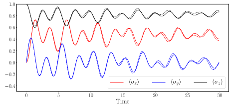
Figure 5: Bloch vector components $\langle\sigma_{i}(t)\rangle={\rm tr}[\varrho_{S}(t)\sigma_{i}]$ vs dimensionless time for the exact dynamics (solid line) and the learning-based prediction (dotted line).

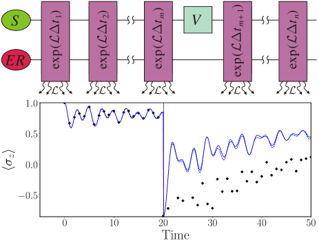
Figure 6: Compatibility of the process tensor formalism with a coherent control gate $V$ applied to the system (top). Example of non-Markovian qubit dynamics with a quick control gate $V=\sigma_{x}$ applied at $t^{\prime}=20$ (bottom): exact solution (solid line), estimated solution within the Markovian embedding approach (dotted line), solution within the full process tomography approach (dots).

Importantly, the formalism of Markovian embedding is compatible with a control operation on system $S$, say, a quick unitary transformation $\varrho_{S}(t^{\prime})\rightarrow V\varrho_{S}(t^{\prime})V^{{\dagger}}$ at time moment $t^{\prime}$. After the operation, $\varrho_{S}(t)={\rm tr}_{ER}\big{\{}\exp[(t-t^{\prime}){\cal L}_{S+ER}]\varrho_{S+ER}(t^{\prime})\big{\}}$. The result is in good agreement with the exact dynamics (Fig. 6), thus opening an avenue toward efficient control and manipulation of non-Markovian quantum systems. In contrast, the conventional process tomography cannot take such a control operation into account: its prediction $\Phi_{S}(t)\Phi_{S}(t^{\prime})^{-1}[V\varrho_{S}(t^{\prime})V^{{\dagger}}]$ differs from $\varrho_{S}(t)$ because of the system-environment correlations supplemental ; gessner-2011 ; rivas-2014 ; milz-2019 , see Fig. 6.

Conclusions.—

We proposed a method to learn the Markovian embedding for non-Markovian quantum evolution. The primary information needed is the outcomes of successive projective measurements on the system. Correlations in the measurements at different times indicate non-Markovianity and allow for the reconstruction of memory effects. The decay of correlations between spaced-in-time measurements enables the reconstruction of relaxation effects. Both memory and relaxation phenomena are taken into account by the generator ${\cal L}_{S+ER}$ acting on the system and the effective reservoir of finite dimension. Our algorithm estimates ${\cal L}_{S+ER}$ and does not exploit the full tomography of either states or processes. Learnability of the algorithm is tested on a dataset for the non-Markovian qubit dynamics. The presented approach enables to take control on the system into consideration, which is impossible with conventional tomographic techniques.

SUPPLEMENTAL MATERIAL

.1 Derivation of the likelihood function gradient

The likelihood function $p({E_{i}}_{i=1}^{n})$ can be rewritten in many alternative ways with the help of the forward propagation operators $\widetilde{\varrho}_{S+ER}(t_{i})$ and the backward propagation operators ${\cal E}_{S+ER}(t_{i})$. In fact, $\widetilde{\varrho}_{S+ER}(t_{i})$ is the subnormalized state of $S+ER$ at time moment $t_{i}$ such that ${\rm tr}[\widetilde{\varrho}_{S+ER}(t_{m})]=p(\{E_{i}\}_{i=1}^{m})$. The total likelihood for $n$ outcomes equals $p(\{E_{i}\}_{i=1}^{n})={\rm tr}[\widetilde{\varrho}_{S+ER}(t_{n})]={\rm tr}[\widetilde{\varrho}_{S+ER}(t_{n})I_{S+ER}]={\rm tr}[\widetilde{\varrho}_{S+ER}(t_{n}){\cal E}_{S+ER}(t_{n})]$, where we have introduced the “initial” condition for backward propagation ${\cal E}_{S+ER}(t_{n})=I_{S+ER}$.

Forward propagation is given by the recurrence relation

$$\widetilde{\varrho}_{S+ER}(t_{i+1})=E_{i}\Phi[\widetilde{\varrho}_{S+ER}(t_{i})]E_{i}={\rm tr}_{A}\big{[}E_{i}\otimes I_{A}\,U(H)\,\widetilde{\varrho}_{S+ER}(t_{i})\otimes\varrho_{A}U^{{\dagger}}(H)\,E_{i}\otimes I_{A}\big{]}$$ (8)

with $\widetilde{\varrho}_{S+ER}(0)=\varrho_{S+ER}(0)$. The last equality in (8) is due to the Stinespring dilation for the channel $\Phi$ exploiting an ancilla $A$ of dimension $d_{A}=(d_{S}d_{ER})^{2}$ (the maximum Kraus rank for the channel $\Phi$ Holevo ). Tensor diagram for Eq. (8) is depicted in Fig. 7. Ancillary systems $A$ play the role of particles colliding with $S+ER$ (see, e.g., fsp-2020 ).

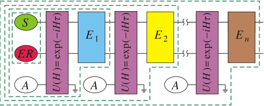
Figure 7: Extended tensor network for the forward propagation.

Similarly, the operator ${\cal E}_{S+ER}(t_{m})$ propagates backward, i.e., in the Heisenberg picture, and is given by the recurrence relation

$${\cal E}_{S+ER}(t_{i-1})=\Phi^{{\dagger}}[E_{i}{\cal E}_{S+ER}(t_{i})E_{i}]={\rm tr}_{A}\big{[}U^{{\dagger}}(H)\,(E_{i}{\cal E}_{S+ER}(t_{i})E_{i}\otimes I_{A})U(H)\,(I_{S+ER}\otimes\varrho_{A})\big{]}$$ (9)

with ${\cal E}_{S+ER}(t_{n})=I_{S+ER}$. The last equality in (9) explicitly uses the Stinesping dilation for the dual channel $\Phi^{{\dagger}}$. Tensor diagram for Eq. (9) is depicted in Fig. 8.

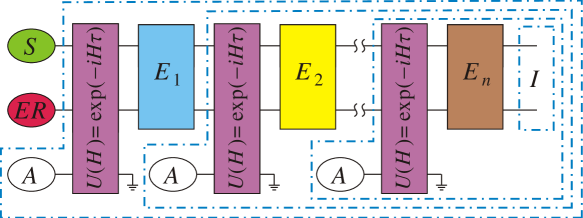
Figure 8: Extended tensor network for the backward propagation.

Merging the forward and backward propagations at a fixed time $t_{m}$, we express the likelihood function in many various though equivalent forms, namely,

$$p(\{E_{i}\}_{i=1}^{n}|H) = {\rm tr}\left[\widetilde{\varrho}_{S+ER}(t_{m}){\cal E}_{S+ER}(t_{m})\right]\quad\forall m=0,\ldots,n,\ t_{0}=0$$ (10)

$$= {\rm tr}\big{[}U(H)\,\widetilde{\varrho}_{S+ER}(t_{m-1})\otimes\varrho_{A}\,U^{{\dagger}}(H)\,\,E_{m}\,{\cal E}_{S+ER}(t_{m})\,E_{m}\otimes I_{A}\big{]}\quad\forall m=1,\ldots,n.$$

The latter expression (10) is a “sandwich” composed of the forward propogation till time $t_{m-1}$ [the state $\widetilde{\varrho}_{S+ER}(t_{m-1})$], the backward propagation till time $t_{m}$ [the operator ${\cal E}_{S+ER}(t_{m})$], and the unitary transformation $U(H)\,\cdot\,U^{{\dagger}}(H)$ followed by the $m$th measurement in between. Since the likelihood function is the $n$-degree monomial with respect to both operators $U(H)$ and $U^{{\dagger}}(H)$, we readily express its gradient operator as follows:

$$\frac{\partial p(\{E_{i}\}_{i=1}^{n}|H)}{\partial H_{\mu\nu}}=\sum_{m=1}^{n}{\rm tr}\bigg{\{}E_{m}{\cal E}_{S+ER}(t_{m})E_{m}\otimes I_{A}\bigg{[}\frac{\partial U(H)}{\partial H_{\mu\nu}}\,\widetilde{\varrho}_{S+ER}(t_{m-1})\otimes\varrho_{A}U^{{\dagger}}(H)+U(H)\widetilde{\varrho}_{S+ER}(t_{m-1})\otimes\varrho_{A}\frac{\partial U^{{\dagger}}(H)}{\partial H_{\mu\nu}}\bigg{]}\bigg{\}}.$$ (11)

The operator $\frac{\partial p(\{E_{i}\}_{i=1}^{n}|H)}{\partial H}$ is Hermitian provided the Hamiltonian $H$ is Hermitian. The derivative $\frac{\partial U(H)}{\partial H}=\left.\frac{\partial U(H+V)}{\partial V}\right|_{V=0}$. We use the perturbation expansion $\exp[-i(H+V)\tau]=\exp(-iH\tau)T_{\leftarrow}\exp\left[-i\int_{0}^{\tau}\exp(iHt^{\prime})V\exp(-iHt^{\prime})dt^{\prime}\right]=\exp(-iH\tau)-i\exp(-iH\tau)\int_{0}^{\tau}\exp(iHt^{\prime})V\exp(-iHt^{\prime})dt^{\prime}+o(V)$ and the spectral decomposition $H=\sum_{k}\lambda_{k}|\psi_{k}\rangle\langle\psi_{k}|$ to get

$$\frac{\partial U(H)}{\partial H_{\mu\nu}}=\left(\frac{\partial U^{{\dagger}}(H)}{\partial H_{\mu\nu}}\right)^{{\dagger}}=\sum_{k,l}\frac{e^{-i\lambda_{k}\tau}-e^{-i\lambda_{l}\tau}}{\lambda_{k}-\lambda_{l}}\langle\psi_{k}|\mu\rangle\langle\nu|\psi_{l}\rangle\,|\psi_{k}\rangle\langle\psi_{l}|.$$ (12)

Finally, we find the gradient of the logarithmic likelihood $\log p({E_{i}}_{i=1}^{n}|H)$ with respect to the unknown parameters $H_{\mu\nu}$:

$$\frac{\partial\log p(\{E_{i}\}_{i=1}^{n}|H)}{\partial H_{\mu\nu}}=\frac{1}{p(\{E_{i}\}_{i=1}^{n}|H)}\,\frac{\partial p(\{E_{i}\}_{i=1}^{n}|H)}{\partial H_{\mu\nu}}.$$ (13)

Note that (13) is insensitive to the normalization of $p(\{E_{i}\}_{i=1}^{n}|H)$, which significantly simplifies the calculation.

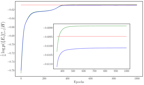
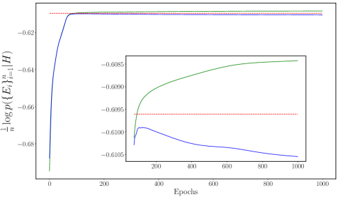
Figure 9: Learning curves: The regularized logarithmic likelihood for the training set (green, upper curve) and the regularized logarithmic likelihood for the validation set (blue, lower curve) vs. number of epochs in Adam algorithm Adam . The dimension of the effective reservoir $d_{ER}=2$ (left) and $d_{ER}=6$ (right). Horizontal line is the theoretical value for the data generated.

.2 Details on the learning algorithm

At item 1 of the algorithm, we initialize the model by randomly choosing the factorized state $\varrho_{S+ER}(0)=\varrho_{S}(0)\otimes\varrho_{ER}(0)$ and the factorized Hamiltonian $H=H_{S+ER}\otimes I_{A}$. Starting with a Hamiltonian, which is factorized with respect to $S+ER$ and $A$, fastens the learning process of memory effects. Otherwise, the correlations between $S+ER$ and $A$ induce irreducible decoherence and dissipation on $S+ER$ that smear out the memory effects.

Typical learning curves in Fig. 9 show how the logarithmic likelihood for the training set increases during the learning process and approaches the theoretical prediction, whereas the likelihood for the validation set starts to decrease after some point in the case of overfitting ($d_{ER}=6$). We test multiple variations of the batch size and the Adam optimizer parameters Adam (used at step 6 of the learning algorithm) to determine the fastest algorithm convergence. The tuned parameters are $\beta_{1}=0.9$, $\beta_{2}=0.95$, $\epsilon=10^{-4}$, the learning rate is $10^{-3}$, the batch size is $10^{3}$.

.3 Details on overfitting

The greater the dimension of the effective reservoir $d_{ER}$, the greater the likelihood for the training set [see Fig. 4(a) in the main text]. However, this leads to overfitting because the likelihood for the validation set starts decreasing with the growth of $d_{ER}$ above the optimal value. A discrepancy between the likelihood for the training set and that for the validation set is a direct indication of the bias-variance tradeoff in machine learning Bishop . Fig. 10 demonstrates the effect of overfitting on the quality of the estimated open dynamics for the example studied. Non-optimal hyperparameter $d_{ER}=6$ leads to redundant oscillations in the predicted dynamics (as opposed to the optimal value $d_{ER}=2$).

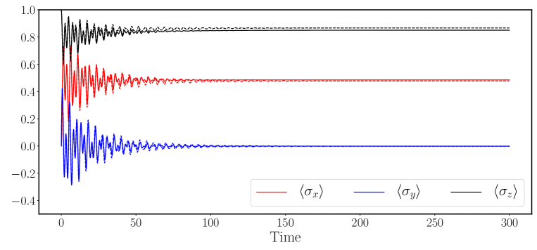
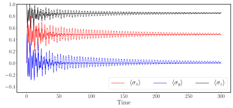
Figure 10: Components $\langle\sigma_{i}(t)\rangle={\rm tr}[\varrho(t)\sigma_{i}]$, $i=x,y,z$, of the system Bloch vector vs. dimensionless time for the exact open dynamics at a long time scale (solid line) and the corresponding learning-based prediction (dotted line) for $d_{ER}=2$ (optimal, top panel) and $d_{ER}=6$ (not optimal, bottom panel).

Fig. 4(b) in the main text illustrates the perfect overfitting of the learning algorithm if the dimension of the effective reservoir $d_{ER}=d_{S}^{n}$, where $n$ is the number of projectors in the data set $\{E_{i}\}_{i=1}^{n}$. Recall that $E_{i}=P_{i}\otimes I_{ER}$, with $P_{i}=\ket{\varphi_{k_{i}}^{(i)}}\bra{\varphi_{k_{i}}^{(i)}}$ being a pure state of $S$. Consider the $n$-partite environment of the form

$$\varrho_{E}=P_{1}\otimes P_{2}\otimes\ldots\otimes P_{n}$$ (14)

and the time-independent unitary transformation for $S+E$

$$W=\exp(-iH\tau)={\sf SHIFT}\cdot{\sf SWAP},$$ (15)

$${\sf SWAP}=\sum{i,j=1}^{d_{S}}\ket{i}_{S}\!\bra{j}\otimes\ket{j}\bra{i}\otimes I_{2\ldots n},$$ (16)

$${\sf SHIFT}=I_{S}\otimes\sum_{i_{1},\ldots,i_{n}=1}^{d_{S}}\ket{i_{2}}\bra{i_{1}}\otimes\ket{i_{1}}\bra{i_{2}}\otimes\ket{i_{2}}\bra{i_{3}}\otimes\ldots\otimes\ket{i_{1}}\bra{i_{n}}.$$ (17)

Note that $\varrho_{S}(\tau)={\rm tr}_{E}(W\varrho_{S}(0)\otimes\varrho_{E}W^{{\dagger}})=P_{1}$ so the first projective measurement on the system in the basis $\ket{\varphi_{k_{1}}^{(1)}}$ would produce the specific outcome ($P_{1}$) with certainty, i.e., with probability 1. The state of environment after the first measurement on the system is

$$\varrho_{E}(\tau)=P_{2}\otimes P_{3}\otimes\ldots\otimes P_{n}\otimes\varrho_{S}(0).$$ (18)

Therefore, $\varrho_{S}(2\tau)={\rm tr}_{E}(W\varrho_{S}(\tau)\otimes\varrho_{E}(\tau)W^{{\dagger}})=P_{2}$, i.e., the outcome for effect $P_{2}$ will be observed with certainty. The state of environment after the first measurement on the system is

$$\varrho_{E}(2\tau)=P_{3}\otimes\ldots\otimes P_{n}\otimes\varrho_{S}(0)\otimes P_{1}.$$ (19)

One can continue the same line of reasoning until all $n$ measurements are performed. As a result we get

$$p(\{E_{i}\}_{i=1}^{n})=\prod_{i=1}^{n}{\rm tr}[\varrho_{S}(i\tau)P_{i}]=1$$ (20)

and the final state of the environment is

$$\varrho_{E}(n\tau)=\varrho_{S}(0)\otimes P_{1}\ldots\otimes P_{n-1}.$$ (21)

This scenario corresponds to the perfect overfitting and yields the logarithmic likelihood $\log p(\{E_{i}\}_{i=1}^{n})=0$ [depicted in the top right corner of Fig. 4(a) in the main text].

However, if more than $n$ measurements in random bases are performed, then the proposed effective reservoir of dimension $d_{S}^{n}$ fails in reproducing the results perfectly. In fact, continue the process above with an extended series of measurements $\{E_{i}\}_{i=n+1}^{2n}$, then

$$p(\{E_{i}\}_{i=n+1}^{2n})={\rm tr}[\varrho_{S}(0)P_{n+1}]\prod_{i=1}^{n-1}{\rm tr}[P_{i}P_{n+i+1}].$$ (22)

If the measurement bases are chosen randomly (Haar measure), then the average $\braket{{\rm tr}[P_{i}P_{n+i+1}]}=\frac{1}{d_{S}}$. Concavity of the logarithm implies

$$\lim_{n\rightarrow\infty}\frac{1}{n}\log p(\{E_{i}\}_{i=n+1}^{2n})\leq\log\left[\lim_{n\rightarrow\infty}\frac{1}{n}\left({\rm tr}[\varrho_{S}(0)P_{n+1}]+\sum_{i=1}^{n-1}{\rm tr}[P_{i}P_{n+i+1}]\right)\right]=\log\frac{1}{d_{S}}.$$ (23)

In other words, the regularized logarithmic likelihood on the validation set $\{E_{i}\}_{i=n+1}^{2n}$ tends to a value not exceeding $\log\frac{1}{d_{S}}$, which is approximately $-0.69$ for $d_{S}=2$ [see the bottom right corner of Fig. 4(a) in the main text].

.4 Details on the hyperparameter $d_{ER}$

In general, the hyperparameter $d_{ER}$ is tuned in such a way that the likelihood on the validation set achieves its maximum. Tuning is reasonable to perform in the vicinity of the physical estimate luchnikov-2019

$$d_{ER}(\epsilon)=\min_{0<\alpha<1}\frac{\sqrt{1-\alpha}}{\epsilon^{\alpha/2(1-\alpha)}}\exp\left[n\gamma T\,\frac{(\gamma\tau)^{\alpha-1}-\alpha}{1-\alpha}\right],$$ (24)

where $\epsilon$ is the desired accuracy of open dynamics, $n$ is the effective subsystem’s number of degrees of freedom interacting with the reservoir ($n\leq d_{S}^{2}$), $\gamma$ is the coupling strength (between the open system and the reservoir), $T$ is the reservoir correlation time, and $\tau$ is the minimal timescale for the open system dynamics (the inverse of the cutoff frequency for the reservoir spectral function).

For some physical systems $d_{ER}$ is defined by the very reservoir structure. For instance, the nuclear spin $I=1$ in nitrogen ${}^{14}N$ is as an effective reservoir for the electronic spin qubit in a nitrogen-vacancy center in diamond haase-2018 , which implies $d_{ER}=2I+1=3$.

.5 Details on the data generation

The synthetic training set $\{E_{i}\}_{i=1}^{n}$ is generated in a non-Markovian composite bipartite collision model lorenzo-2017 . We consider a bipartite system that successively interacts with qubit subenvironments $R$ during collision time $\Delta t$, with the bipartite system being composed of the very open qubit system under study $S$ and one auxiliary qubit system $S_{1}$, see Fig. 11. The composite bipartite collision model lorenzo-2017 allows to find the system evolution $\varrho_{S}(t)={\rm tr}_{S_{1}}[\varrho_{S+S_{1}}(t)]$ intervened by measurements on the system.

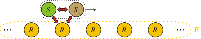
Figure 11: Composite bipartite collision model used in data generation. The infinite environment $E$ is composed of identical qubit subenvironments $R$ each with a density matrix $\varrho_{R}=\frac{1}{2}(I+\sigma_{z})$. Three thick red arrows denote the interaction with Hamiltonian (25) for a period $\Delta t$.

We fix the (dimensionless) interaction Hamiltonian between $S$, $S_{1}$, and $R$ in the form

$$H_{S+S_{1}+R}=\sigma_{z}\otimes I\otimes I+\sigma_{x}\otimes I\otimes I+I\otimes\sigma_{z}\otimes I+I\otimes\sigma_{x}\otimes I+\sigma_{z}\otimes\sigma_{z}\otimes I+0.3\,I\otimes\sigma_{z}\otimes\sigma_{z}+0.3\,I\otimes\sigma_{y}\otimes\sigma_{y}+0.3\,I\otimes\sigma_{x}\otimes\sigma_{x}.$$ (25)

The coefficients in the interaction Hamiltonian correspond to the case when strong memory effects are present in the evolution whereas the relaxation time is much longer than the recurrence time of memory effects — the hardest open dynamics to reconstruct. Each collision results in the transformation $\varrho_{S+S_{1}}(t+\Delta t)={\rm tr}_{R}\big{[}\exp(-iH_{S+S_{1}+R}\Delta t)\varrho_{S+S_{1}}(t)\otimes\varrho_{R}\exp(iH_{S+S_{1}+R}\Delta t)\big{]}$.

To simulate projective measurements in random bases we proceed as follows. Suppose the qubit system is in the state $\varrho_{S}(t_{i})$ at time $t_{i}=i\tau$. We randomly choose a direction ${\bf r}^{(i)}\in\mathbb{R}^{3}$, $|{\bf r}^{(i)}|=1$, on a Bloch ball and calculate eigenvectors $|\varphi_{+}^{(i)}\rangle$ and $|\varphi_{-}^{(i)}\rangle$ of the polarization operator $r_{x}^{(i)}\sigma_{x}+r_{y}^{(i)}\sigma_{y}+r_{z}^{(i)}\sigma_{z}$, where $(\sigma_{x},\sigma_{y},\sigma_{z})$ is the conventional set of Pauli operators. The transformation $\{\pm\}\rightarrow|\varphi_{\pm}^{(i)}\rangle\langle\varphi_{\pm}^{(i)}|$ is an observable at time $t_{i}=i\tau$. One of the two measurement outcomes $\{\pm\}$ is accepted, with the probability to accept the result $+$ being $\langle\varphi_{+}^{(i)}|\varrho_{S}(t)|\varphi_{+}^{(i)}\rangle$. As a result, one of the operators $|\varphi_{\pm}^{(i)}\rangle\langle\varphi_{\pm}^{(i)}|\otimes I_{ER}$ is accepted as $E_{i}$. Observation of the outcome $\pm$ in the $i$th measurement of the system results in the transformation $\varrho_{S+S_{1}}\rightarrow|\varphi_{\pm}^{(i)}\rangle\langle\varphi_{\pm}^{(i)}|\otimes\varrho_{S_{1}}^{\pm}/{\rm tr}[\varrho_{S_{1}}^{\pm}]$, where $\varrho_{S_{1}}^{\pm}=(\langle\varphi_{\pm}^{(i)}|\otimes I_{S_{1}})\varrho_{S+S_{1}}(t)(|\varphi_{\pm}^{(i)}\rangle\otimes I_{S_{1}})$. The measurement is followed by another collision described above, which in turn is followed by a measurement, and so on until the set $\{E_{i}\}_{i=1}^{n}$ is completed.

.6 Variational Bayesian inference approach

In the presented learning algorithm, we maximize the likelihood function and find parameters $H_{\mu\nu}$ encoding the desired generator ${\cal L}_{S+ER}$ for the Markovian embedding. However, the algorithm itself does not provide the error (variance) of parameters $H_{\mu\nu}$. This error can, however, be estimated via the variational Bayesian method as follows. Let $p(H)$ be an a priori distribution for Hamiltonian $H$, say, a uniform distribution on ${\rm Re}H_{\mu\nu}$ and ${\rm Im}H_{\mu\nu}$ within a wide range. For an observed sequence of operators $\{E_{i}\}_{i=1}^{n}$ we get the a posteriori distribution

$$p(H|\{E_{i}\}_{i=1}^{n})=\frac{p(\{E_{i}\}_{i=1}^{n}|H)p(H)}{\int p(\{E_{i}\}_{i=1}^{n}|H)p(H)dH}=\frac{1}{Z}p(\{E_{i}\}_{i=1}^{n}|H)$$ (26)

with some constant $Z$. Although $p(H|\{E_{i}\}_{i=1}^{n})$ is not known precisely, we expect that for sufficiently big data set this distribution can be approximated by a factorized Gaussian distribution

$$Q_{\{\kappa_{\mu\nu},\sigma_{\mu\nu},\varkappa_{\mu\nu},\varsigma_{\mu\nu}\}}(H)=\prod_{\mu,\nu}\left[\frac{1}{\sqrt{2\pi}\,\sigma_{\mu\nu}}\exp\left(-\frac{({\rm Re}H_{\mu\nu}-\kappa_{\mu\nu})^{2}}{2\sigma_{\mu\nu}^{2}}\right)\right]\prod_{\mu,\nu}\left[\frac{1}{\sqrt{2\pi}\,\varsigma_{\mu\nu}}\exp\left(-\frac{({\rm Im}H_{\mu\nu}-\varkappa_{\mu\nu})^{2}}{2\varsigma_{\mu\nu}^{2}}\right)\right],$$ (27)

where the parameters $\kappa_{\mu\nu}+i\varkappa_{\mu\nu}$ define the optimal values $H_{\mu\nu}$ maximizing the likelihood, and the standard deviations $\sigma_{\mu\nu}$ and $\varsigma_{\mu\nu}$ define the accuracy of parameter estimation for the real and imaginary part of $H_{\mu\nu}$, respectively. If the number of measurements $n\rightarrow\infty$, then $\sigma_{\mu\nu}\rightarrow 0$ and $\varsigma_{\mu\nu}\rightarrow 0$. Our goal is to find $\sigma_{\mu\nu}$ and $\varsigma_{\mu\nu}$ for a finite $n$. To do so we minimize the Kullback–Leibler divergence $D_{\rm KL}$ of $p(H|\{E_{i}\}_{i=1}^{n})$ from $Q_{\{\kappa_{\mu\nu},\sigma_{\mu\nu},\varkappa_{\mu\nu},\varsigma_{\mu\nu}\}}(H)$, where $D_{\rm KL}(q(x)\,||\,p(x))=\int dx\,q(x)[\log q(x)-\log p(x)]$. One can readily see that

$$D_{\rm KL}\left(Q_{\{\kappa_{\mu\nu},\sigma_{\mu\nu},\varkappa_{\mu\nu},\varsigma_{\mu\nu}\}}(H)\,||\,p(H|\{E_{i}\}_{i=1}^{n})\right)=D_{\rm KL}\left(Q_{\{\kappa_{\mu\nu},\sigma_{\mu\nu},\varkappa_{\mu\nu},\varsigma_{\mu\nu}\}}(H)\,||\,p(\{E_{i}\}_{i=1}^{n}|H)\right)+\log Z.$$ (28)

Since $Z$ is independent of $H$ or either of $\kappa_{\mu\nu},\sigma_{\mu\nu},\varkappa_{\mu\nu},\varsigma_{\mu\nu}$, the minimization of (28) reduces to the minimization of $D_{\rm KL}\left(Q_{\{\kappa_{\mu\nu},\sigma_{\mu\nu},\varkappa_{\mu\nu},\varsigma_{\mu\nu}\}}(H)\,||\,p(\{E_{i}\}_{i=1}^{n}|H)\right)$. Using the explicit form of the Gaussian distribution, we come the so-called reparameterization trick molchanov-2017 ; kingma-2013 : the minimization of $D_{\rm KL}\left(Q_{\{\kappa_{\mu\nu},\sigma_{\mu\nu},\varkappa_{\mu\nu},\varsigma_{\mu\nu}\}}(H)\,||\,p(\{E_{i}\}_{i=1}^{n}|H)\right)$ is equivalent to the minimization of the functional

$$F(\kappa_{\mu\nu},\sigma_{\mu\nu},\varkappa_{\mu\nu},\varsigma_{\mu\nu})=-\sum_{\mu\nu}\log\sigma_{\mu\nu}-\sum_{\mu\nu}\log\varsigma_{\mu\nu}-\mathbb{E}_{\scriptsize\begin{array}[]{c}\xi_{\mu\nu}\sim{\cal N}(0,1)\\ \zeta_{\mu\nu}\sim{\cal N}(0,1)\\ \end{array}}\left[p\Big{(}\{E_{i}\}_{i=1}^{n}\Big{|}\{\kappa_{\mu\nu}+\xi_{\mu\nu}\sigma_{\mu\nu}+i(\varkappa_{\mu\nu}+\zeta_{\mu\nu}\varsigma_{\mu\nu})\}_{\mu,\nu}\Big{)}\right],$$ (29)

where ${\cal N}(0,1)$ is the standard normal distribution. The expectation value in the right hand side of Eq. (29) is readily estimated by sampling from the standard normal distribution, i.e., $\mathbb{E}_{\xi\sim{\cal N}(0,1)}f(\xi)\approx\frac{1}{M}\sum_{j=1}^{M}f(\xi^{(j)})$, where $\xi^{(j)}$ is a sample from ${\cal N}(0,1)$. With such an estimation at hand, the minimization of (29) is readily performed numerically, which yields the optimal approximation $Q_{\{\kappa_{\mu\nu}^{\rm opt},\sigma_{\mu\nu}^{\rm opt},\varkappa_{\mu\nu}^{\rm opt},\varsigma_{\mu\nu}^{\rm opt}\}}(H)$.

A posteriori distribution of the system density operator $\varrho_{S}(t)$ at time $t$ is

$$p\big{(}\varrho_{S}(t)\big{|}\{E_{i}\}_{i=1}^{n}\big{)} = \int\delta\left\{\varrho_{S}(t)-{\rm tr}_{ER}\left[\exp\big{(}t{\cal L}_{S+ER}(H)\big{)}\varrho_{S+ER}(0)\right]\right\}p(H|\{E_{i}\}_{i=1}^{n})\,dH$$ (30)

$$\approx \int\delta\left\{\varrho_{S}(t)-{\rm tr}_{ER}\left[\exp\big{(}t{\cal L}_{S+ER}(H)\big{)}\varrho_{S+ER}(0)\right]\right\}Q_{\{\kappa_{\mu\nu}^{\rm opt},\sigma_{\mu\nu}^{\rm opt},\varkappa_{\mu\nu}^{\rm opt},\varsigma_{\mu\nu}^{\rm opt}\}}(H)\,dH.$$

Sampling from the distribution (30) for a given time $t$, we get the standard deviation for matrix elements of the system density operator $\varrho_{S}(t)$. The results are depicted in Fig. 12 for short and long timescales. The maximum standard deviation for matrix elements of the estimated density operator equals 0.025 at time moments $t=50$.

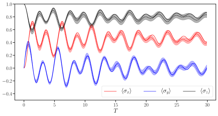
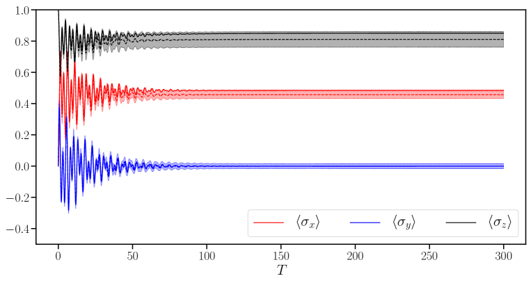
Figure 12: Exact solution (solid line) and the Bayesian inference (dotted line, $d_{ER}=2$) for the open qubit dynamics in terms of the Bloch vector at a short timescale (top panel) and a long time scale (bottom panel). Shaded area depicts the standard deviation for the Bloch vector components.

.7 Error estimation

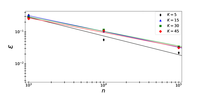
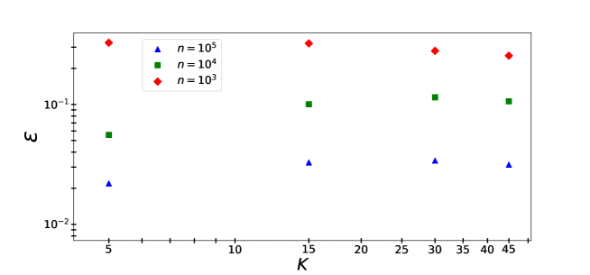
Figure 13: Average error (34) for the estimated quantum dynamical map $\Phi_{S}(t)$ with $d_{ER}=2$ vs. the number of projective measurements used (top panel), vs. the number $K$ of time moments analyzed, $t_{i}=i$, $i=1,\ldots,K$ (bottom panel).

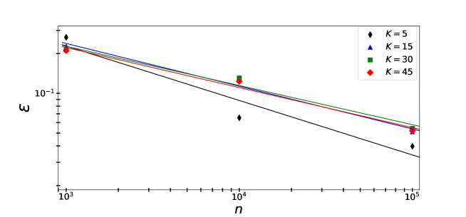
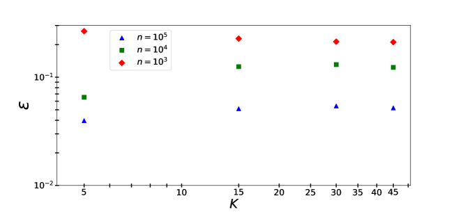
Figure 14: Average error (36) for the Bayesian inference for the quantum dynamical map $\Phi_{S}(t)$ with $d_{ER}=2$ vs. the number of projective measurements used (top panel), vs. the number $K$ of time moments analyzed, $t_{i}=i$, $i=1,\ldots,K$ (bottom panel).

The presented learning algorithm uses $n$ projective measurements on the system to estimate the Markovian embedding for the non-Markovian system dynamics. This reconstruction results in the process tensor depicted in Fig. 2 in the main text. As a result, we can infer a desired number of channels $\Phi_{S}(t_{i})$, $i=1,\ldots,K$, for the system dynamics from time $0$ to time $t_{i}$ by formula

$$\Phi_{S}(t)[\varrho_{S}(0)]={\rm tr}_{ER}\left[\exp(t{\cal L}_{S+ER})[\varrho_{S}(0)\otimes\varrho_{ER}(0)]\right].$$ (31)

By the Choi–Jamiołkowski isomorphism, all the information about the channel $\Phi_{S}(t)$ is contained in the matrix $\Omega_{\Phi_{S}(t)}$ defined through (see, e.g., Holevo ; filippov-jms-2019 )

$$\Omega_{\Phi_{S}(t)}=(\Phi_{S}(t)\otimes{\rm Id}_{S})[\ket{\psi_{+}}\bra{\psi_{+}}],$$ (32)

where $\ket{\psi_{+}}=\frac{1}{\sqrt{d_{S}}}\sum_{i=1}^{d_{S}}\ket{i}\otimes\ket{i}$ is the maximally entangled state.

Provided the exact dynamical map $\Phi_{S}^{\rm exact}(t)$ is known, the error in estimating the channel $\Phi_{S}(t)$ can therefore be expressed as

$$\epsilon\big{(}\Phi_{S}(t)\big{)}=\frac{1}{2}\|\Omega_{\Phi_{S}(t)}-\Omega_{\Phi_{S}^{\rm exact}(t)}\|_{1},$$ (33)

where $\|A\|_{1}={\rm tr}\sqrt{A^{{\dagger}}A}$. The average error in estimating a set of channels $\{\Phi_{S}(t_{i})\}_{i=1}^{K}$ equals

$$\varepsilon(\{\Phi_{S}(t_{i})\}_{i=1}^{K})=\frac{1}{K}\sum_{i=1}^{K}\epsilon(\Phi_{S}(t_{i}))=\frac{1}{2K}\sum_{i=1}^{K}\|\Omega_{\Phi_{S}(t_{i})}-\Omega_{\Phi_{S}^{\rm exact}(t_{i})}\|_{1}.$$ (34)

Fig. 13 shows the error $\varepsilon(\{\Phi_{S}(t_{i})\}_{i=1}^{K})$ scales with $n$ as $\frac{1}{\sqrt{n}}$ and is almost independent of $K$.

If the exact quantum dynamical map $\Phi_{S}(t)$ is not known (as it takes place for experimental data), the error is estimated via the variational Bayesian inference approach. In full analogy with the previous section, we get the posterior distribution of channels $\Phi_{S}(t)$ and the corresponding Choi operators, namely,

$$p(\Omega_{\Phi_{S}(t)}|\{E_{i}\}_{i=1}^{n})\approx\int\delta\left\{\Omega_{\Phi_{S}(t)}-\frac{1}{d_{S}}\sum_{i,j=1}^{d_{S}}{\rm tr}_{ER}\left[\exp(t{\cal L}_{S+ER})[\ket{i}\bra{j}\otimes\varrho_{ER}(0)]\right]\otimes\ket{i}\bra{j}\right\}Q_{\{\kappa_{\mu\nu}^{\rm opt},\sigma_{\mu\nu}^{\rm opt},\varkappa_{\mu\nu}^{\rm opt},\varsigma_{\mu\nu}^{\rm opt}\}}(H)\,dH.$$ (35)

By sampling from the latter distribution, we calculate the average error for the proposed learning algorithm

$$\varepsilon(\{\Phi_{S}(t_{i})\}_{i=1}^{K})=\frac{1}{2K}\sum_{i=1}^{K}\mathbb{E}\left[\|\Omega_{\Phi_{S}(t_{i})}-\Omega_{\mathbb{E}\Phi_{S}(t_{i})}\|_{1}\right],$$ (36)

where $\mathbb{E}\Phi_{S}(t_{i})$ is the mean Bayesian inference (obtained via averaging over samples). Fig. 14 shows that, in this case, the error $\varepsilon(\{\Phi_{S}(t_{i})\}_{i=1}^{K})$ scales with $n$ as $\frac{1}{\sqrt{n}}$ and is almost independent of $K$.

.8 Comparison with the full process tomography

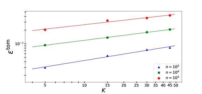
Figure 15: Average error (37) for the tomographic inference of the quantum dynamical map $\Phi_{S}(t)$ vs. the total number of projective measurements used (top panel), vs. the number $K$ of time moments analyzed, $t_{i}=i$ (bottom panel).

The standard quantum-process tomography exploits an ensemble of identically prepared quantum systems corresponding to a given experimental setting (see, e.g., the review knee-2018 ). Suppose the total number of available projective measurements is $n$. As we are interested in reconstructing $K$ channels $\{\Phi_{S}(t_{i})\}_{i=1}^{K}$ with the minimal possible average error, the number of projective measurements per each channel equals $\frac{n}{K}$. The theory of process tomography bogdanov-2013 ; haah-2017 predicts the reconstruction error $\epsilon\sim\frac{d_{S}^{4}}{\sqrt{n/K}}$ in this case. In what follows, we confirm this prediction numerically.

Ref. knee-2018 proposes an algorithm that maximizes the likelihood for the observed measurement outcomes and provides a legitimate (trace preserving and completely positive) estimate for $\Phi_{S}^{\rm tom}(t_{i})$. Dealing with a qubit dynamical map ($d_{S}=2$), one needs to prepare the system in one of four pure initial states $\{\varrho_{S}^{(j)}(0)\}_{j=1}^{4}$, where $\varrho_{S}^{(1)}(0)=\ket{0}\bra{0}$, $\varrho_{S}^{(2)}(0)=\ket{1}\bra{1}$, $\varrho_{S}^{(3)}(0)=\frac{1}{2}(\ket{0}+\ket{1})(\bra{0}+\bra{1})$, $\varrho_{S}^{(4)}(0)=\frac{1}{2}(\ket{0}+i\ket{1})(\bra{0}-i\bra{1})$. Then the randomly chosen state $\varrho_{S}^{(j)}(0)$ is evolved through the channel $\Phi_{S}^{\rm tom}(t_{i})$ and is measured with the help of an 8-outcome positive operator-valued measure (POVM) with effects $\{F_{k}\}_{k=1}^{8}$, where $F_{2m-1}=\frac{1}{4}\varrho_{S}^{(m)}(0)$ and $F_{2m}=\frac{1}{4}[I-\varrho_{S}^{(m)}(0)]$, $m=1,\ldots,4$. After the measurement outcome is read out, the environment should be reset to the initial (thermal equilibrium) state and the system should be again prepared in one of the states $\{\varrho_{S}^{(j)}(0)\}_{j=1}^{4}$. This is a challenge in real experimental setup (especially in the case of strong coupling between the system and environment) and a disadvantage as compared to our proposed scheme of sequential measurements with no environment resets. Suppose, however, that the experiment is repeated $n/K$ times. This results in integers $\{n_{jk}\}_{j=1,\ldots,4,\ k=1,\ldots,8}$, which quantify how many times the outcome $k$ is observed provided the system is prepared in the state $\varrho_{S}^{(j)}(0)$. Clearly, the relative frequencies $\frac{4Kn_{jk}}{n}$ tend to probabilities $p_{jk}={\rm tr}\Big{[}\Phi_{S}^{\rm tom}(t_{i})[\varrho_{S}^{(j)}(0)]F_{k}\Big{]}$ if $n\rightarrow\infty$. The authors of Ref. knee-2018 maximize the likelihood $\prod_{jk}p_{jk}^{n_{jk}}$ with respect to $\Phi_{S}(t_{i})$ and find the best estimate $\Phi_{S}^{\rm tom}(t_{i})$ for the quantum channel. We use the solver in Ref. knee-2018 to find $\Phi_{S}^{\rm tom}(t_{i})$ for a given number of measurements $n/K$.

Suppose the exact dynamical map $\Phi_{S}(t)$ is known, then the average reconstruction error equals

$$\varepsilon^{\rm tom}(\{\Phi_{S}(t_{i})\}_{i=1}^{K})=\frac{1}{2K}\sum_{i=1}^{K}\|\Omega_{\Phi_{S}^{\rm tom}(t_{i})}-\Omega_{\Phi_{S}^{\rm exact}(t_{i})}\|_{1}.$$ (37)

Fig. 15 shows the error $\varepsilon^{\rm tom}(\{\Phi_{S}(t_{i})\}_{i=1}^{K})$ scales as $\sqrt{K/n}$, which is in strong contrast to Fig. 13.

.9 Details on the coherent control

Within the process tensor formalism for Markovian embedding, we are able to describe the action of coherent control pulses on the system experiencing a non-Markovian dynamics. Suppose the system is subjected to a quick unitary transformation $\varrho_{S}(t^{\prime})\rightarrow V\varrho_{S}(t^{\prime})V^{{\dagger}}$ at time moment $t^{\prime}$. The corresponding tensor diagram is depicted in Fig. 16.

The estimated system dynamics after the operation is given by the equation $\varrho_{S}(t)={\rm tr}_{ER}\big{\{}\exp[(t-t^{\prime}){\cal L}_{S+ER}]\varrho_{S+ER}(t^{\prime})\big{\}}$. Fig. 17 illustrates the qubit evolution for $V=\sigma_{x}$ and $t^{\prime}=20$. The exact dynamics and the estimated dynamics are in good agreement with each other.

Suppose the full process tomography is performed for time moments $t_{1},t_{2},\ldots,t_{K}$ and the maps $\Phi_{S}(t_{1}),\Phi_{S}(t_{2}),\ldots,\Phi_{S}(t_{K})$ are reconstructed precisely. The dynamics within the time interval $[t_{i},t_{i+1}]$ is given by the intermediate map $\Lambda(t_{i+1},t_{i})=\Phi_{S}(t_{i+1})\Phi_{S}^{-1}(t_{i})$. Denoting $t_{0}=0$, we note that $\Phi_{S}(t_{j})=\Lambda(t_{j},t_{j-1})\cdots\Lambda(t_{2},t_{1})\Lambda(t_{1},t_{0})=:\bigcirc_{i=0}^{j-1}\Lambda(t_{i+1},t_{i})$, i.e., the dynamics is described by concatenation of intermediate maps. If a coherent control gate $V$ is applied at time moment $t_{m}$, then the concatenation approach yields

$$\varrho_{S}(t_{l})=\left\{\begin{array}[]{ll}\bigcirc_{i=0}^{l-1}\Lambda(t_{i+1},t_{i})[\varrho_{S}(0)]=\Phi_{S}(t_{l})[\varrho_{S}(0)]&\text{if~{}~{}}l<m,\\ \bigcirc_{i=m}^{l-1}\Lambda(t_{i+1},t_{i})\Big{[}V\left(\bigcirc_{j=0}^{m-1}\Lambda(t_{j+1},t_{j})[\varrho_{S}(0)]\right)V^{{\dagger}}\Big{]}=\Phi_{S}(t_{l})\Phi_{S}^{-1}(t_{m})\Big{[}V\Phi_{S}(t_{m})[\varrho_{S}(0)]V^{{\dagger}}\Big{]}&\text{if~{}~{}}l\geq m.\\ \end{array}\right.$$ (38)

This approach results in the dynamics depicted in Fig. 17 by dots. Clearly, Eq. (38) is not able to reproduce the system dynamics after the control gate is applied because $\Phi_{S}(t)\Phi_{S}(t^{\prime})^{-1}[V\varrho_{S}(t^{\prime})V^{{\dagger}}]\neq\varrho_{S}(t)$ for $t>t^{\prime}$ due to the system-environment correlations gessner-2011 ; rivas-2014 ; milz-2019 .

Non-monotonicity of the trace distance $\frac{1}{2}\|\varrho_{S}^{\prime}(t)-\varrho_{S}^{\prime\prime}(t)\|_{1}$ for some initial states $\varrho_{S}^{\prime}(0)$ and $\varrho_{S}^{\prime\prime}(0)$ is a clear indication of non-Markovianity BLP , and the learned Markovian embedding reproduces such a non-monotonic behavior quite well lvgf-2019 .

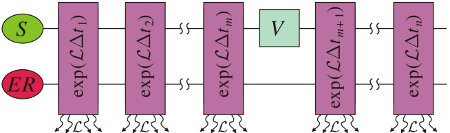
Figure 16: Process tensor formalism is compatible with a coherent control gate $V$ applied to the system at time $t^{\prime}=t_{m}$.

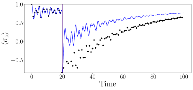
Figure 17: Non-Markovian qubit dynamics with a quick control gate $V=\sigma_{x}$ applied at $t^{\prime}=20$: exact solution (solid line), estimated solution within the Markovian embedding approach (dotted line), solution (38) within the full process tomography approach (dots).