Wave breaking and formation of dispersive shock waves in a defocusing nonlinear optical material

Abstract

We theoretically describe the quasi one-dimensional transverse spreading of a light beam propagating in a nonlinear optical material in the presence of a uniform background light intensity. For short propagation distances the pulse can be described within a nondispersive (geometric optics) approximation by means of Riemann’s approach. For larger distances, wave breaking occurs, leading to the formation of dispersive shocks at both edges of the beam. We describe this phenomenon within Whitham modulation theory, which yields an excellent agreement with numerical simulations. Our analytic approach makes it possible to extract the leading asymptotic behavior of the parameters of the shock, setting up the basis for a theory of non-dissipative weak shocks.

I Introduction

It has long been realized that light propagating in a nonlinear medium was amenable to a hydrodynamic treatment, see e.g., Refs. Tal65 ; ASK66 ; ASK67 . In the case of a defocusing nonlinearity, this rich analogy has not only triggered experimental research, but also made it possible to get an intuitive understanding of observations such as the formation of rings in the far field beyond a nonlinear slab Akh67 ; Har97 , of dark solitons Emp87 ; Kro88 ; Wei88 , vortices Are91 ; Vau96 ; Voc18 , wave breaking Rot89 ; Gho07 and dispersive shock waves Cou04 ; wkf-07 ; Bar07 ; Fat14 ; Xu16 ; Xu17 , of spontaneously self-accelerated Airy beams Kar15 , of optical event horizon Ela12 , ergo-regions Voc17 and stimulated Hawking radiation Dro18 , of sonic-like dispersion relation Voc15 ; Fon18 and superfluid motion Mic18 . Very similar phenomena have also been observed in the neighboring fields of cavity polaritons and of Bose-Einstein condensation of atomic vapors. They all result from the interplay between nonlinearity and dispersion, whose effects become prominent near a gradient catastrophe region.

In this work we present a theoretical treatment of a model configuration which has been realized experimentally in a one-dimensional situation in Refs. wkf-07 ; Xu16 : the nonlinear spreading of a region of increased light intensity in the presence of a uniform constant background. In the absence of background, and for a smooth initial intensity pattern, the spreading is mainly driven by the nonlinear defocusing and can be treated analytically in some simple cases Tal65 . The situation is more interesting in the presence of a constant background: the pulse splits in two parts, each eventually experiencing nonlinear wave breaking, leading to the formation of a dispersive shock wave (DSW) which cannot be described within the framework of perturbation theory, even if the region of increased intensity corresponds to a weak perturbation of the flat pedestal. This scenario indeed fits with the hydrodynamic approach of nonlinear light propagation, and is nicely confirmed by the experimental observations of Refs. wkf-07 ; Xu16 . Although the numerical treatment of the problem is relatively simple kgk-04 ; El07 ; Conf12 , a theoretical approach to both the initial splitting of the pulse and the subsequent shock formation requires a careful analysis. The goal of this article is to present such an analysis. A most significant outcome of our detailed treatment is a simple asymptotic description of some important shock parameters. This provides a non-dissipative counterpart of the usual weak viscous shock theory (see, e.g., Ref. whitham-74 ) and paves the way for a quantitative experimental test of our predictions.

The paper is organized as follows: In Sec. II we present the model and the set-up we aim at studying. After a brief discussion of shortcomings of the linearized approach, the spreading and splitting stage of evolution is accounted for in Sec. III within a dispersionless approximation which holds when the pulse region initially presents no large intensity gradient. It is well known that in such a situation the light flow can be described by hydrodynamic-like equations which can be cast into a diagonal form for two new position and time-dependent variables — the so called Riemann invariants. The difficulty here lies in the fact that the splitting involves simultaneous variations of both of them: one does not have an initial simple wave within which one of the Riemann invariants remains constant, as occurs for instance in a similar uni-directional propagation case modeled by the Korteweg-de Vries equation (see, e.g., Ref. Iso18 ). We treat the problem in Secs. III.1 and III.2 using an extension of the Riemann method due to Ludford Lud52 (also used in Ref. For2009 ) and compare the results with numerical simulations in Sec. III.3. During the spreading of the pulse, nonlinear effects induce wave steepening which results in a gradient catastrophe and wave breaking. After the wave breaking time, dispersive effects can no longer be omitted, a shock is formed, and in this case we resort to Whitham modulation theory whitham-74 to describe the time evolution of the pulse. Such a treatment was initiated long ago by Gurevich and Pitaevskii gp-73 , and since that time it has developed into a powerful method with numerous applications (see, e.g., the review article eh-16 ). Here there is an additional complexity which lies—as for the initial non-dispersive stage of evolution—in the fact that two of the (now four) Riemann invariants which describe the modulated nonlinear oscillations vary in the shock region. Such a wave has been termed as “quasi-simple” in Ref. gkm-89 , and a thorough treatment within Whitham theory has been achieved in the Korteweg-de Vries case in Refs. Gur91 ; Gur92 ; Kry92 ; ek-93 . We generalize in Sec. IV this approach to the nonlinear Schrodinger equation (NLS) which describes light propagation in the nonlinear Kerr medium (see also Ref. El2009 ). An interesting outcome of our theoretical treatment is the asymptotic determination of experimentally relevant parameters of the dispersive shock, see Sec. V. In Sec. VI we present the full Whitham treatment of the after-shock evolution and compare the theoretical results with numerical simulations. We present in Sec. VII a panorama the different regimes we have identified, and discuss how our approach can be used to get a simple estimate of the contrast of the fringes of the DSW. This should be helpful for determining the best experimental configuration for studying the wave breaking phenomenon and the subsequent dispersive shock. Our conclusions are presented in Sec. VIII.

II The model and the linear approximation

In the paraxial approximation, the stationary propagation of the complex amplitude $A(\vec{r}\,)$ of the electric field of a monochromatic beam is described by the equation (see, e.g., Ref. LL8 )

$${\rm i}\partial_{z}A=-\frac{1}{2n_{0}k_{0}}\vec{\nabla}^{2}_{\!\perp}A-k_{0}\delta n\,A\;.$$ (1)

In this equation, $n_{0}$ is the linear refractive index, $k_{0}=2\pi/\lambda_{0}$ is the carrier wave vector, $z$ is the coordinate along the beam, $\vec{\nabla}^{2}_{\perp}$ the transverse Laplacian and $\delta n$ is a nonlinear contribution to the index. In a non absorbing defocusing Kerr nonlinear medium one can write $\delta n=-n_{2}|A|^{2}$, with $n_{2}>0$.

We define dimensionless units by choosing a reference intensity $I_{\rm ref}$ and introducing the nonlinear length $z_{\rm\scriptscriptstyle NL}=(k_{0}n_{2}I_{\rm ref})^{-1}$ and the transverse healing length $\xi_{\perp}=(z_{\rm\scriptscriptstyle NL}/n_{0}k_{0})^{1/2}$. We consider a geometry where the transverse profile is translationally invariant and depends on a single Cartesian coordinate. One thus writes $\vec{\nabla}^{2}_{\!\perp}=\xi_{\perp}^{-2}\partial_{x}^{2}$ where $x$ is the dimensionless transverse coordinate and we define an effective “time” $t=z/z_{\rm\scriptscriptstyle NL}$. The quantity $\psi(x,t)=A/\sqrt{I_{\rm ref}}$ is then a solution of the dimensionless NLS equation

$${\rm i}\,\psi_{t}=-\tfrac{1}{2}\psi_{xx}+|\psi|^{2}\psi\;.$$ (2)

In the following we consider a system with a uniform background light intensity, on top of which an initial pulse is added at the entrance of the nonlinear cell. The initial $\psi(x,t=0)$ is real (i.e., no transverse velocity or, in optical context, no focusing of the light beam at the input plane), with a dimensionless intensity $\rho(x,t)=|\psi|^{2}$ which departs from the constant background value (which we denote as $\rho_{0}$) only in the region near the origin where it forms a bump. To be specific, we consider the typical case where

$$\rho(x,0)=\begin{cases}\rho_{0}+\rho_{1}(1-x^{2}/x_{0}^{2})&\mbox{if}\quad|x|<x_{0},\\ \rho_{0}&\mbox{if}\quad|x|\geq x_{0}.\end{cases}$$ (3)

We will denote as $\rho_{m}=\rho_{0}+\rho_{1}$ the maximal density of the initial profile. It would be natural to choose the reference light intensity $I_{\rm ref}$ to be equal to the background one, in this case one would have $\rho_{0}=1$. However, we prefer to be more general and to allow for values of $\rho_{0}$ different from unity.

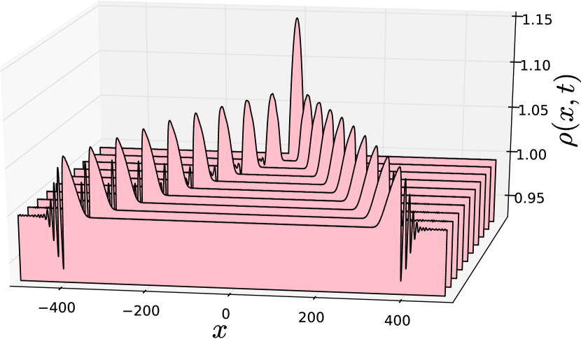
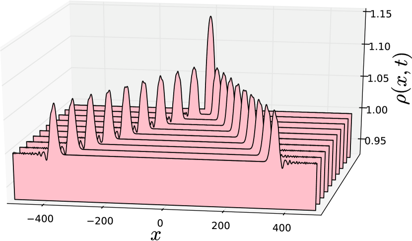
Figure 1: Density profiles $\rho(x,t)$ for an initial condition $u(x,0)=0$ and $\rho(x,0)$ given by (3) with $\rho_{0}=1$, $\rho_{1}=0.15$ and $x_{0}=20$. The upper part of the figure represents the results of the numerical solution of Eq. (2), while the lower part corresponds to the linearized version (4). The profiles are plotted from time $t=0$ to $t=360$ with a time step equal to 40.

We stress here the paramount importance of nonlinear effects at large “time” (i.e., for large propagation distance in the nonlinear medium). Even for a bump which weakly departs from the background density, a perturbative approach fails after the wave breaking time. This is illustrated in Fig. 1 which compare numerical simulations of the full equation (2) with its linearized version. The linearized treatment is obtained by writing $\psi(x,t)=\exp(-{\rm i}\rho_{0}t)(\sqrt{\rho_{0}}+\delta\psi(x,t))$ and assuming that $|\delta\psi|^{2}\ll\rho_{0}$ which yields the following evolution equation

$${\rm i}\,\partial_{t}\delta\psi=-\tfrac{1}{2}\partial_{x}^{2}\delta\psi+\rho_{0}(\delta\psi+\delta\psi^{*})\;,$$ (4)

and then $\rho(x,t)\simeq\rho_{0}+\sqrt{\rho_{0}}(\delta\psi+\delta\psi^{*})$. In the case illustrated in Fig. 1, the initial profile has, at its maximum, a weak 15% density increase with respect to the background. The initial splitting of the bump if correctly described by the linearized approach, but after the wave breaking time the linearized evolution goes on predicting a roughly global displacement of the two humps at constant velocity (with additional small dispersive corrections) and clearly fails to reproduce both the formation of DSWs and the stretching of the dispersionless part of the profile (which reaches a quasi-triangular shape).

III The dispersionless stage of evolution

In view of the shortcomings of the linearized approximation illustrated in Fig. 1, we include nonlinear effects at all stages of the dynamical study of the model. By means of the Madelung substitution

$$\psi(x,t)=\sqrt{\rho(x,t)}\exp\left({\rm i}\int^{x}u(x^{\prime},t)\,dx^{\prime}\right)$$ (5)

the NLS equation (2) can be cast into a hydrodynamic-like form for the density $\rho(x,t)$ and the flow velocity $u(x,t)$:

$$\begin{split}\rho_{t}+(\rho u)_{x}=0\;,\\ u_{t}+uu_{x}+\rho_{x}+\left(\frac{\rho_{x}^{2}}{8\rho^{2}}-\frac{\rho_{xx}}{4\rho}\right)_{x}=0\;.\end{split}$$ (6)

These equations are to be solved with the initial conditions (3) and $u(x,0)=0$.

The last term of the left hand-side of the second of Eqs. (6) accounts for the dispersive character of the fluid of light. In the first stage of spreading of the bump, if the density gradients of the initial density are weak (i.e., if $x_{0}\gg\mathrm{max}\{\rho_{0}^{-1/2},\rho_{1}^{-1/2}\}$), the effects of dispersion can be neglected, and the system (6) then simplifies to

$$\rho_{t}+(\rho u)_{x}=0\;,\quad u_{t}+uu_{x}+\rho_{x}=0\;.$$ (7)

These equations can be written in a more symmetric form by introducing the Riemann invariants

$$\lambda^{\pm}(x,t)=\frac{u(x,t)}{2}\pm\sqrt{\rho(x,t)}\;,$$ (8)

which evolve according to the system [equivalent to (7)]:

$$\partial_{t}\lambda^{\pm}+v_{\pm}(\lambda^{-},\lambda^{+})\,\partial_{x}\lambda^{\pm}=0\;,$$ (9)

with

$$v_{\pm}(\lambda^{-},\lambda^{+})=\tfrac{1}{2}(3\lambda^{\pm}+\lambda^{\mp})=u\pm\sqrt{\rho}\;.$$ (10)

The Riemann velocities (10) have a simple physical interpretation for a smooth velocity and density distribution: $v_{+}$ ($v_{-}$) corresponds to a signal which propagates downstream (upstream) at the local velocity of sound $c=\sqrt{\rho}$ and which is dragged by the background flow $u$.

The system (9) can be linearized by means of the hodograph transform (see, e.g., Ref. kamch-2000 ) which consists in considering $x$ and $t$ as functions of $\lambda^{+}$ and $\lambda^{-}$. One readily obtains

$$\partial_{\pm}x-v_{\mp}\partial_{\pm}t=0,$$ (11)

where $\partial_{\pm}\equiv\partial/\partial\lambda^{\pm}$. One introduces two auxiliary (yet unknown) functions $W_{\pm}(\lambda^{+},\lambda^{-})$ such that

$$x-v_{\pm}(\lambda^{-},\lambda^{+})\,t=W_{\pm}(\lambda^{-},\lambda^{+}).$$ (12)

Inserting the above expressions in (11) shows that the $W^{\pm}$’s are solution of Tsarev equations Tsa91

$$\begin{split}&\frac{\partial_{-}W_{+}}{W_{+}-W_{-}}=\frac{\partial_{-}v_{+}}{v_{+}-v_{-}},\\ &\frac{\partial_{+}W_{-}}{W_{+}-W_{-}}=\frac{\partial_{+}v_{-}}{v_{+}-v_{-}}.\end{split}$$ (13)

From Eqs. (10) and (13) one can verify that $\partial_{-}W_{+}=\partial_{+}W_{-}$, which shows that $W_{+}$ and $W_{-}$ can be sought in the form

$$W_{\pm}=\partial_{\pm}\chi,$$ (14)

where $\chi(\lambda^{-},\lambda^{+})$ plays the role of a potential. Substituting expressions (14) in one of the Tsarev equations shows that $\chi$ is a solution of the Euler-Poisson equation

$$\frac{\partial^{2}\chi}{\partial\lambda^{+}\partial\lambda^{-}}-\frac{1}{2\,(\lambda^{+}-\lambda^{-})}\left(\frac{\partial\chi}{\partial\lambda^{+}}-\frac{\partial\chi}{\partial\lambda^{-}}\right)=0,$$ (15)

which can be written under the standard form

$$\frac{\partial^{2}\chi}{\partial\lambda^{+}\partial\lambda^{-}}+a(\lambda^{-},\lambda^{+})\frac{\partial\chi}{\partial\lambda^{+}}+b(\lambda^{-},\lambda^{+})\frac{\partial\chi}{\partial\lambda^{-}}=0,$$ (16)

with

$$a(\lambda^{-},\lambda^{+})=-b(\lambda^{-},\lambda^{+})=-\frac{1}{2\,(\lambda^{+}-\lambda^{-})}.$$ (17)

III.1 Solution of the Euler-Poisson equation

One can use Riemann’s method to solve Eq. (16) in the ($\lambda^{+}$, $\lambda^{-}$)–plane which we denote below as the “characteristic plane”. We follow here the procedure exposed in Refs. Lud52 ; For2009 which applies to non-monotonous initial distributions, such as the one corresponding to Eq. (3).

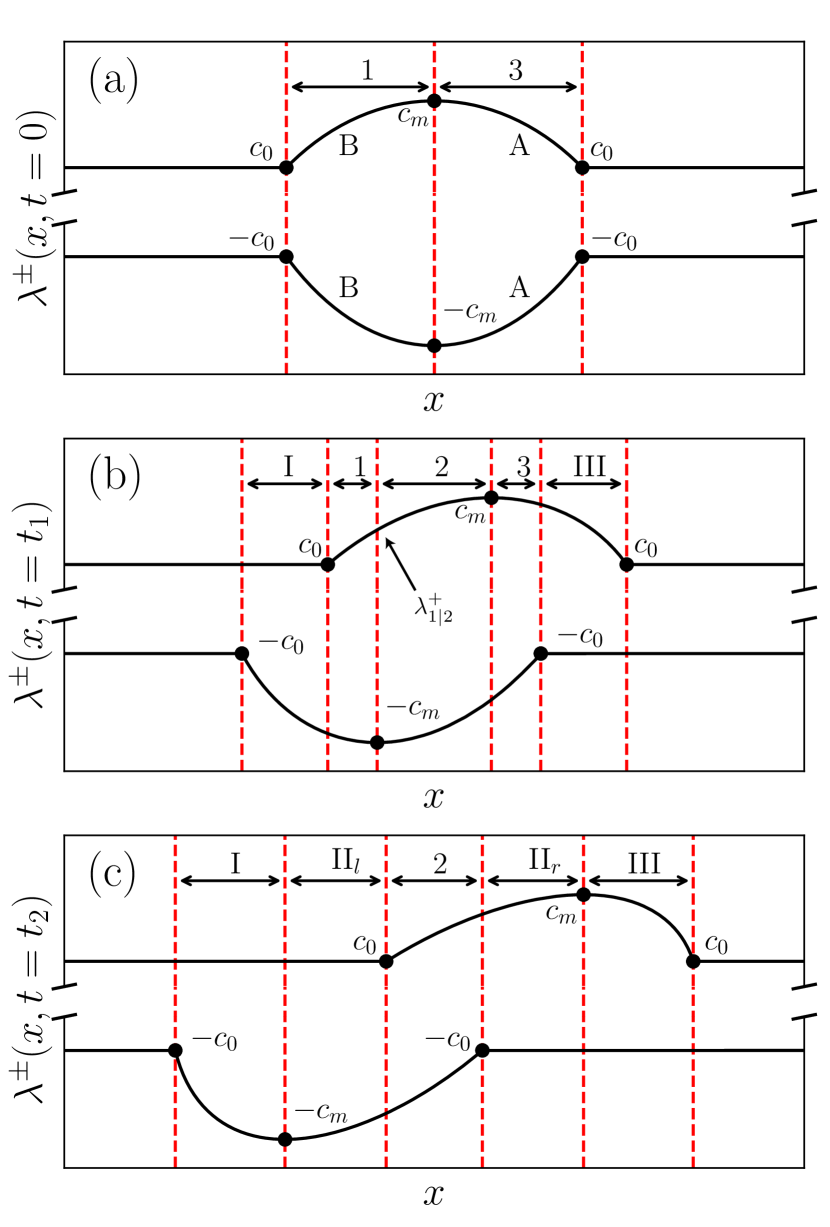
Figure 2: Sketch of the distributions $\lambda^{\pm}(x,t)$ at several times. In each panel the upper solid curve represent $\lambda^{+}$ (always larger than $c_{0}$), and the lower one $\lambda^{-}$ (always lower than $-c_{0}$), both plotted as functions of $x$. Panel (a) corresponds to the initial distribution, in which part B corresponds to region 1 and part A to region 3 (see the text). Two subsequent relevant stages of evolution are represented in panels (b) and (c). They correspond to times $t_{1}<t_{\rm\scriptscriptstyle SW}(c_{m})<t_{2}$, where $t_{\rm\scriptscriptstyle SW}(c_{m})$ is defined in Sec. III.2 (see also Fig. 4). For $t>0$, $\lambda^{+}$ ($\lambda^{-}$) moves to the right (to the left) and part B of $\lambda^{+}$ starts to overlap with part A of $\lambda^{-}$. This behavior initially leads to the configuration represented in panel (b) where a new region (labeled region 2) has appeared. For later convenience, we spot in this panel the value $\lambda^{+}_{1|2}(t_{1})$ of the Riemann invariant $\lambda^{+}$ at the boundary between regions 1 and 2 (see the discussion in Sec. III.3). For longer time (panel (c)), region 2 remains while regions 1 and 3 vanish and new simple wave regions II_l and II_r appear. At even larger times (not represented), region 2 also vanishes and only simple-wave regions remain: the initial pulse has split in two simple-wave pulses propagating in opposite directions.

We first schematically depict in Fig. 2 the initial spatial distributions $\lambda^{\pm}(x,0)$ of the Riemann invariants (upper panel), and their later typical time evolution (lower panels). We introduce notations for some special initial values of the Riemann invariants: $\lambda^{\pm}(-x_{0},0)=\lambda^{\pm}(x_{0},0)=\pm\sqrt{\rho_{0}}=\pm c_{0}$ and $\lambda^{\pm}(0,0)=\pm\sqrt{\rho_{m}}=\pm c_{m}$. We also define as part A (part B) the branch of the distribution of the $\lambda^{\pm}$’s which is at the right (at the left) of the extremum. All these notations are summarized in Fig. 2(a).

At a given time, the $x$ axis can be considered as divided in five domains, each requiring a specific treatment. Each region is characterized by the behavior of the Riemann invariant and is identified in the two lower panels of Fig. 2. The domains in which both Riemann invariants depend on position are labeled by arabic numbers, the ones in which only one Riemann invariant depends on $x$ are labeled by capital roman numbers. For instance, in region III, $\lambda^{+}$ is a decreasing function of $x$ while $\lambda^{-}=-c_{0}$ is a constant; in region 3, $\lambda^{+}$ is decreasing while $\lambda^{-}$ is increasing; in region 2 both are increasing, etc.

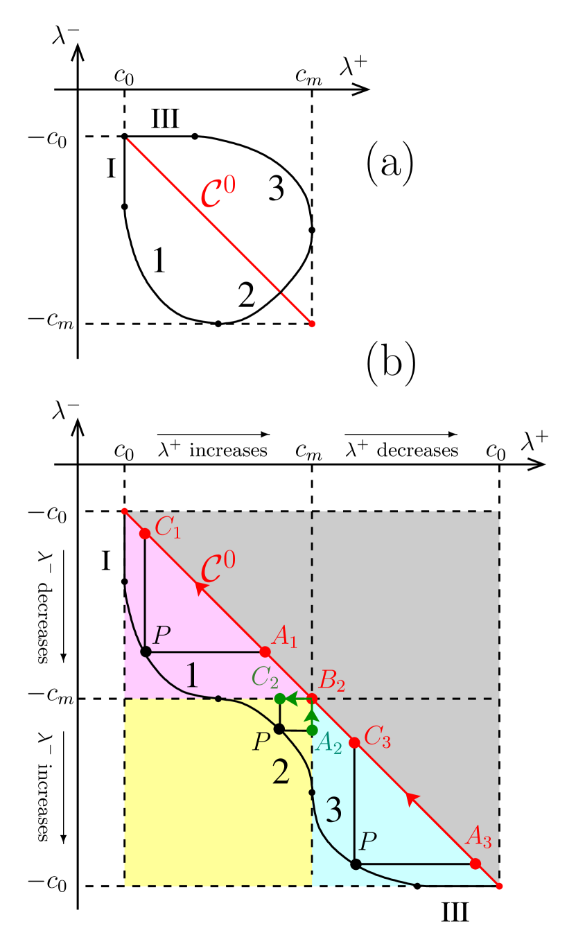
Figure 3: (a) Behavior of the Riemann invariants in the characteristic plane at a given time $t$. (b) The same curve on the four-sheeted unfolded surface. The red curve $\mathcal{C}^{\,0}$ corresponds to the initial condition [$\lambda^{-}(x,0)=-\lambda^{+}(x,0)$]. At later time, the relation between $\lambda^{+}(x,t)$ and $\lambda^{-}(x,t)$ is given by the black solid curve which is denoted as $\mathcal{C}^{\,t}$ in the main text. A generic point $P$ of $\mathcal{C}^{\,t}$ has coordinates ($\lambda^{+}$, $\lambda^{-}$) and points $C_{1},A_{1},B_{2},C_{3},A_{3}$ lie on the initial curve $\mathcal{C}^{\,0}$. Points $A_{2}$ and $C_{2}$ lie on a boundary between two regions. The arrows indicate the direction of integration in Eq. (21) and (28). In our problem, the whole gray shaded domain above ${\cal C}^{0}$ is unreachable.

The values of the Riemann invariants at time corresponding to the central panel of Fig. (2) are represented in the characteristic plane in Fig. 3(a). In this plot the straight solid lines correspond to the simple wave regions (I and III) while the curvy lines corresponds to regions where both Riemann invariants depend on position: the domains 1, 2 and 3. In each of these three domains the solution $\chi$ of the Euler-Poisson equation has a different expression. In order to describe these three branches, following Ludford Lud52 , we introduce several sheets in the characteristic plane by unfolding the domain $[c_{0},c_{m}]\times[-c_{m},-c_{0}]$ into a four times larger region as illustrated in Fig. 3(b). The potential $\chi(\lambda^{-},\lambda^{+})$ can now take a different form in each of the regions labeled 1, 2 and 3 in Fig. 3(b) and still be considered as single-valued.

We consider a flow where initially $u(x,0)=0$, this implies that $\lambda^{+}(x,0)=-\lambda^{-}(x,0)$. This condition defines the curve of initial conditions of our problem in the characteristic plane. It is represented by a red solid line denoted as $\mathcal{C}^{\,0}$ in Fig. 3. We remark here that the whole region above $\mathcal{C}^{\,0}$ — shaded in Fig. 3(b) — is unreachable for the initial distribution we consider: for instance the upper shaded triangle in region 1 would correspond to a configuration in which $\lambda^{+}_{{\rm region}1}(x,t)>|\lambda^{-}_{{\rm region}1}(x,t)|$, which does not occur in our case, see Fig. 2(b).

Before establishing the expression for $\chi$ is the three relevant regions of Fig. 3 it is convenient to define the inverse functions of the initial $\lambda$ profiles in both parts A and B of Fig. 2(a). The symmetry of the initial conditions makes it possible to use the same functions for $\lambda^{+}\in[c_{0},c_{m}\,]$ and for $\lambda^{-}\in[-c_{m},-c_{0}\,]$:

$$\begin{cases}x=w^{\scriptscriptstyle\rm A}(\lambda^{\pm})=x_{0}\sqrt{1-\frac{\displaystyle(\lambda^{\pm})^{2}-\rho_{0}}{\displaystyle\rho_{m}-\rho_{0}}}\quad\text{if}\;\;x>0,\\[5.69054pt] x=w^{\scriptscriptstyle\rm B}(\lambda^{\pm})=-x_{0}\sqrt{1-\frac{\displaystyle(\lambda^{\pm})^{2}-\rho_{0}}{\displaystyle\rho_{m}-\rho_{0}}}\quad\text{if}\;\;x<0.\end{cases}$$ (18)

For $t=0$, using Eqs. (12) and (14), the boundary conditions read

$$\left.\frac{\partial\chi}{\partial\lambda^{\pm}}\right|_{\lambda^{\pm}(x,t=0)}=x=w^{{\rm\scriptscriptstyle A}/{\rm\scriptscriptstyle B}}(\lambda^{\pm}),$$ (19)

where the superscript B holds in region 1 (when $x<0$) and A holds in region 3 ($x>0$). Formula (19) requires some explanation: its left-hand side is a function of two variables $\lambda^{+}$ and $\lambda^{-}$ which is evaluated for $\lambda^{-}=-\lambda^{+}$; its right-hand side is expressed by the same function in terms of $\lambda^{+}$ or $\lambda^{-}$ since the function $w^{{\rm\scriptscriptstyle A}}$ and $w^{{\rm\scriptscriptstyle B}}$ depend only on the square of their argument. The boundary conditions (19) corresponds to a potential $\chi$ which takes the following form along ${\cal C}^{\,0}$:

$$\begin{split}\chi^{(n)}(\lambda^{-}=-\lambda^{+},\lambda^{+})=&\int_{c_{0}}^{\lambda^{+}}\!\!\!\!w^{{\rm\scriptscriptstyle A}/{\rm\scriptscriptstyle B}}(r)\,dr\\ &+\int_{-c_{0}}^{\lambda^{-}}\!\!\!\!w^{{\rm\scriptscriptstyle A}/{\rm\scriptscriptstyle B}}(r)\,dr,\end{split}$$ (20)

where $n=1$ or 3 and, in the right hand side, and the superscript A (B) holds when $n=3$ ($n=1$). For the specific initial condition we consider ($u(x,0)\equiv 0$ and $\rho(x,0)$ an even function of $x$), $w^{{\rm\scriptscriptstyle A}}$ and $w^{{\rm\scriptscriptstyle B}}$ are even functions and thus our choice of integration constants yields $\chi=0$ along ${\cal C}^{\,0}$.

Let us now consider a point $P$, lying either in region 1 or 3 (the case of region 2 is considered later), with coordinates $(\lambda^{+},\lambda^{-})$ in the characteristic plane. We introduce points $A_{1}$, $A_{3}$, $C_{1}$ and $C_{3}$ which are located on the curve $\mathcal{C}^{\,0}$, with geometrical definitions obvious from Fig. 3(b). Note the different subscripts for $C$ and $A$: subscript 1 (3) is to be used if $P$ is in region 1 (3). One can obtain the value of $\chi$ at the point $P$ from Riemann’s method (see, e.g. Ref. Som64 ), the general solution reads

$$\begin{split}\chi^{(n)}(P)=&\frac{1}{2}\chi(C_{n})R(C_{n})+\frac{1}{2}\chi(A_{n})R(A_{n})\\ &-\int_{A_{n}}^{C_{n}}V\,dr+U\,ds,\end{split}$$ (21)

with

$$\begin{split}&U(s,r)=\frac{1}{2}\left(R\,\frac{\partial\chi}{\partial s}-\chi\,\frac{\partial R}{\partial s}\right)+aR\,\chi,\\ &V(s,r)=\frac{1}{2}\left(\chi\,\frac{\partial R}{\partial r}-R\,\frac{\partial\chi}{\partial r}\right)-bR\,\chi,\end{split}$$ (22)

where

$$R(s,r)=\frac{2}{\pi}\sqrt{\frac{r-s}{\lambda^{+}-\lambda^{-}}}\,\mathrm{K}[m(s,r)],$$ (23)

$\mathrm{K}$ being the complete elliptic integral of the first kind and

$$m(s,r)=\frac{(\lambda^{+}-r)\,(\lambda^{-}-s)}{(r-s)\,(\lambda^{+}-\lambda^{-})}.$$ (24)

is the associated parameter (we follow here the convention of Ref. AS ). In our case, the symmetries of the initial profile lead to many simplifications in the above formulas (21) and (22). Along the curve $\mathcal{C}^{\,0}$ one has $\chi=0$. This implies that $\chi^{(n)}(A_{n})=\chi^{(n)}(C_{n})=0$, and along the integration path going from $A_{n}$ to $C_{n}$ one has

$$U=\tfrac{1}{2}\,w^{{\rm\scriptscriptstyle A}/{\rm\scriptscriptstyle B}}(r)\,R(s=-r,r)=-V\;,$$ (25)

where the superscript A (B) holds when $P$ is in region 3 (region 1). Explicit evaluation of expression (21) then yields

$$\chi^{(n)}(P)=\frac{2\,\sqrt{2}}{\pi\,\sqrt{\lambda^{+}-\lambda^{-}}}\int_{-\lambda^{-}}^{\lambda^{+}}\!\!\!\!\sqrt{r}\,\mathrm{K}[m(r)]\,w^{{\rm\scriptscriptstyle A}/{\rm\scriptscriptstyle B}}(r)\,dr,$$ (26)

where

$$m(r)\equiv m(-r,r)=\frac{(\lambda^{+}-r)\,(\lambda^{-}+r)}{2\,r\,(\lambda^{+}-\lambda^{-})}\;.$$ (27)

To calculate $\chi(P)$ in region 2 we define three points: $A_{2}$, $B_{2}$ and $C_{2}$, see Fig. 3(b). Point $B_{2}$ is on the curve $\mathcal{C}^{\,0}$, at the junction between regions 1, 2 and 3. Point $A_{2}$ lies on the characteristic curve $\lambda^{+}=c_{m}$, on the boundary between regions 2 and 3, whereas point $C_{2}$ lies on the characteristic $\lambda^{-}=-c_{m}$, on the boundary between regions 1 and 2. Then, from Eqs. (21) to (24), one can easily find that in region 2

$$\begin{split}\chi^{(2)}(P)&=\chi(B_{2})\,R(B_{2})+\int_{B_{2}}^{C_{2}}\left(\frac{\partial\chi}{\partial r}+b\chi\right)\,R_{1}(r)\,dr\\ &-\int_{A_{2}}^{B_{2}}\left(\frac{\partial\chi}{\partial s}+a\chi\right)\,R_{2}(s)\,ds,\end{split}$$ (28)

where

$$\begin{cases}&R_{1}(r)\equiv\frac{\displaystyle 2}{\displaystyle\pi}\sqrt{\displaystyle\frac{r+c_{m}}{\lambda^{+}-\lambda^{-}}}\,\mathrm{K}[m_{1}(r)],\\[5.69054pt] &m_{1}(r)=\frac{\displaystyle(r-\lambda^{+})\,(c_{m}+\lambda^{-})}{\displaystyle(r-\lambda^{-})\,(\lambda^{+}+c_{m})},\end{cases}$$ (29)

and

$$\begin{cases}&R_{2}(s)=\frac{\displaystyle 2}{\displaystyle\pi}\sqrt{\displaystyle\frac{c_{m}-s}{\lambda^{+}-\lambda^{-}}}\mathrm{K}[m_{2}(s)],\\[5.69054pt] &m_{2}(s)=\frac{\displaystyle(c_{m}-\lambda^{+})\,(\lambda^{-}-s)}{\displaystyle(c_{m}-\lambda^{-})\,(\lambda^{+}-s)}.\end{cases}$$ (30)

Note that in formula (28) one has $\chi(B_{2})=0$ and the value of $\chi$ along the integration lines $B_{2}C_{2}$ and $A_{2}B_{2}$ is known from the previous result (26). After some computation we eventually get the following expression for $\chi(P)$ in region 2:

$$\begin{split}\chi^{(2)}(P)&=\frac{2\,\sqrt{2}}{\pi\,\sqrt{\lambda^{+}-\lambda^{-}}}\left[\int_{c_{m}}^{\lambda^{+}}\!\!\!\!\!\sqrt{r}\,\mathrm{K}[m_{0}(r\,;\lambda^{+})]\,w^{\rm\scriptscriptstyle B}(r)\,dr\right.\\ &\left.+\int_{-\lambda^{-}}^{c_{m}}\sqrt{r}\,\mathrm{K}[m_{0}(r\,;-\lambda^{-})]\,w^{\rm\scriptscriptstyle A}(r)\,dr\right]\\ &+\frac{4\,\sqrt{2}}{\pi^{2}\,\sqrt{\lambda^{+}-\lambda^{-}}}\left[\int_{c_{m}}^{\lambda^{+}}\sqrt{r}\,w^{\rm\scriptscriptstyle B}(r)\,f_{1}(r)\,dr\right.\\ &\left.+\int_{-\lambda^{-}}^{c_{m}}\sqrt{r}\,w^{\rm\scriptscriptstyle A}(r)\,f_{2}(r)\,dr\right],\end{split}$$ (31)

where we have introduced the notations

$$\begin{split}f_{1}(r)&=\int_{\lambda^{+}}^{r}\mathrm{K}[m_{0}(r\,;u)]\,\frac{\partial\mathrm{K}[m_{1}(u)]}{\partial u}\,du\;,\\ f_{2}(r)&=\int_{-\lambda^{-}}^{r}\mathrm{K}[m_{0}(r\,;u)]\,\frac{\partial\mathrm{K}[m_{2}(-u)]}{\partial u}\,du\;,\end{split}$$ (32)

with

$$m_{0}(r;u)=\frac{(r-u)(c_{m}-r)}{2r(u+c_{m})}\;.$$ (33)

In many instances one can actually simplify the above expressions (26) and (31): for reasonable values of $c_{m}$ (chosen to be of same order as $c_{0}$ in our simulations) the elliptic integral $\mathrm{K}(m)$ turns out to be approximately equal to $\pi/2$ for all points $P$ in the three regions. In this case, the exact expressions (26) and (31) can be replaced by a simple approximation $\chi(P)\simeq{\chi}_{\rm app}(P)$ which reads, when $P$ is in region $n=1$ or $3$:

$$\chi^{(n)}_{\rm app}(\lambda_{-},\lambda_{+})=\frac{\sqrt{2}}{\sqrt{\lambda^{+}-\lambda^{-}}}\int_{-\lambda^{-}}^{\lambda^{+}}\!\!\!\!\sqrt{r}\,\,w^{{\rm\scriptscriptstyle A}/{\rm\scriptscriptstyle B}}(r)\,dr,$$ (34)

where the superscript A (B) holds when $n=3$ ($n=1$). When $P$ is in region $2$ one gets:

$$\begin{split}{\chi}^{(2)}_{\rm app}(\lambda_{-},\lambda_{+})&=\frac{\sqrt{2}}{\sqrt{\lambda^{+}-\lambda^{-}}}\int_{c_{m}}^{\lambda^{+}}\sqrt{r}\,w^{\rm\scriptscriptstyle B}(r)\,dr\\ &+\frac{\sqrt{2}}{\sqrt{\lambda^{+}-\lambda^{-}}}\int_{-\lambda^{-}}^{c_{m}}\sqrt{r}\,w^{\rm\scriptscriptstyle A}(r)\,dr.\end{split}$$ (35)

This approximation greatly simplifies the numerical determination of the integrals involved in the solution of the problem. We have checked that it is very accurate in all the configurations we study in the present work. The reason for its validity is easy to understand in regions 1 and 3: the argument of the elliptic integral K in Eq. (26) is zero at the two boundaries of the integration domain ($r=-\lambda^{-}$ and $r=\lambda^{+}$) and reaches a maximum when $r=\sqrt{-\lambda^{-}\lambda^{+}}$, taking the value

$$0\leq m_{\rm max}=\frac{1}{2}\left(1-\frac{2\,\sqrt{-\lambda^{-}\lambda^{+}}}{\lambda^{+}-\lambda^{-}}\right)\leq\frac{1}{2}\;.$$ (36)

As time varies, the largest value of of $m_{\rm max}$ is reached at the point where region 3 disappears, when $\lambda^{+}=c_{m}$ and $\lambda^{-}=-c_{0}$. For $c_{m}/c_{0}\sim 1$ this value is typically much lower than the upper bound $1/2$ of Eq. (36). For instance, in the numerical simulations below, we take $\rho_{0}=0.5$ and $\rho_{m}=2$ one gets accordingly $c_{0}=\sqrt{0.5}$ and $c_{m}=\sqrt{2}$ and the corresponding largest value of $m_{\rm max}$ is about $\simeq 2.9\times 10^{-2}$.

III.2 Simple wave regions

Once $\chi$ has been computed in the domains 1, 2 and 3 where two Riemann invariants depend on position, it remains to determine the value of $\lambda^{+}$ and $\lambda^{-}$ in the simple wave regions. Let us for instance focus on region III, in which $\lambda^{-}=-c_{0}$ and $\lambda^{+}$ depends on $x$ and $t$. The behavior of the characteristics in the $(x,t)$ plane is sketched in Fig. 4.

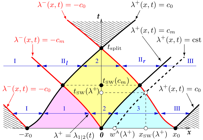
Figure 4: Sketch of the characteristics in the $(x,t)$ plane. The black (red) solid lines are specific characteristics for $\lambda^{+}$ ($\lambda^{-}$) stemming from the edges of the hump and from its maximum. The thick dashed line is a generic characteristics for $\lambda^{+}$. In the hatched regions both Riemann invariants are constant ($\lambda^{\pm}(x,t)=\pm c_{0}$) and the profile is flat. In the colored regions both Riemann invariants depend on position (the color code is the same as in Fig. 3: region 1 is pink, region 2 is yellow, and region 3 is cyan). In the white regions only one Riemann invariant depends on position: one has a simple wave. The different notations are explained in the main text.

One sees in this figure that the characteristic of a given value of $\lambda^{+}$ enters the simple wave region III at a given time which we denote as $t_{\rm\scriptscriptstyle SW}(\lambda^{+})$ and a given position $x_{\rm\scriptscriptstyle SW}(\lambda^{+})$. Beyond this point the characteristic becomes a straight line and the general solution of Eq. (9) for $\lambda^{+}$ is known to be of the form

$$x-v_{+}(-c_{0},\lambda^{+})t=h(\lambda^{+})\;,$$ (37)

where the unknown function $h$ is determined by boundary conditions. From Eq. (12) one sees that just at the boundary between regions 3 and III one has

$$x_{\rm\scriptscriptstyle SW}(\lambda^{+})-v_{+}(-c_{0},\lambda^{+})t_{\rm\scriptscriptstyle SW}(\lambda^{+})=W_{+}^{(3)}(-c_{0},\lambda^{+})\;,$$ (38)

where $W_{+}^{(3)}=\partial_{+}\chi^{(3)}$. This shows that in Eq. (37) the unknown function $h(\lambda^{+})$ is equal to $W_{+}^{(3)}(-c_{0},\lambda^{+})$. The equation of the characteristic in region III thus reads

$$x-v_{+}(-c_{0},\lambda^{+})t=W_{+}^{(3)}(-c_{0},\lambda^{+})\;.$$ (39)

A similar reasoning shows that in region I one has

$$x-v_{-}(\lambda^{-},c_{0})t=W_{-}^{(1)}(\lambda^{-},c_{0})\;.$$ (40)

For time larger than $t_{\rm\scriptscriptstyle SW}(c_{m})$, the regions 1 and 3 disappear and two new simple wave regions appear which we denote as II_l and II_r, see Fig. 4 and also the lower panel of Fig. 2. The same reasoning as above shows that in these regions the characteristics are determined by

$$x-v_{+}(-c_{0},\lambda^{+})t=W_{+}^{(2)}(-c_{0},\lambda^{+})\;,\quad\mbox{in II${}_{r}$,}$$ (41)

and

$$x-v_{-}(\lambda^{-},c_{0})t=W_{-}^{(2)}(\lambda^{-},c_{0})\;,\quad\mbox{in II${}_{l}$.}$$ (42)

III.3 Solution of the dispersionless problem and comparison with numerical simulations

The problem is now solved: having determined $\chi$ in regions 1, 2 and 3 (see Sec. III.1), we obtain $W_{\pm}$ in these regions from Eqs. (14).

$\bullet$ It is then particularly easy to find the values of $\lambda^{+}$ and $\lambda^{-}$ in the simple wave regions. For instance, in region III, one has $\lambda_{-}=-c_{0}$, and for given $x$ and $t$, $\lambda^{+}$ is obtained from Eq. (39). The same procedure is to be employed in the simple wave regions I, II_r and II_l where the relevant equations are then Eqs. (40), (41), (42) respectively.

$\bullet$ To determine the values of $\lambda^{+}$ and $\lambda^{-}$ as functions of $x$ and $t$ in regions 1, 2 and 3 one follows a different procedure which is detailed below, but which essentially consists in the following: for a given time $t$ and a given region $n$ ($n=1$, 2 or 3) one picks one of the possible values of $\lambda^{+}$. From Eqs. (12) $\lambda^{-}$ is then solution of

$$\frac{W_{+}^{(n)}(\lambda^{-},\lambda^{+})-W_{-}^{(n)}(\lambda^{-},\lambda^{+})}{v_{+}(\lambda^{-},\lambda^{+})-v_{-}(\lambda^{-},\lambda^{+})}+t=0\;,$$ (43)

and $x$ is determined by either one of Eqs. (12). So, for given $t$ and $\lambda^{+}$ in region $n$, one has determined the values of $\lambda^{-}$ and $x$. In practice, this makes it possible to associate a couple $(\lambda^{-},\lambda^{+})$ in region $n$ to each $(x,t)$.

The procedure for determining the profile in regions 1, 2, and 3 which has just been explained has to be implemented with care, because the relevant regions to be considered and their boundaries change with time; for instance regions 1 and 3 disappear when $t>t_{\scriptscriptstyle\rm SW}(c_{m})$. It would be tedious to list here all the possible cases and we rather explain the specifics of the procedure by means of an example: the determination of $\lambda^{+}$ and $\lambda^{-}$ in region 1 when $t<t_{\scriptscriptstyle\rm SW}(c_{m})$.

One starts by determining the value of $\lambda^{+}$ along the characteristic $\lambda^{-}=-c_{m}$ at time $t$ (see Fig. 4). This value of $\lambda^{+}$ defines the boundary between regions 1 and 2 and we accordingly denote it as $\lambda^{+}_{1|2}(t)$, it is represented in Fig. 2(b). From Eqs. (12) it is a solution of

$$\frac{W_{+}^{(1)}(-c_{m},\lambda^{+}_{1|2})-W_{-}^{(1)}(-c_{m},\lambda^{+}_{1|2})}{v_{+}(-c_{m},\lambda^{+}_{1|2})-v_{-}(-c_{m},\lambda^{+}_{1|2})}+t=0\;.$$ (44)

We then know that, in region 1, at time $t$, $\lambda^{+}$ takes all possible values between $c_{0}$ and $\lambda^{+}_{1|2}(t)$. Having determined the precise range of variation of $\lambda^{+}$ we can now, for each possible $\lambda^{+}$, determine $\lambda^{-}$ from Eq. (43) (with $n=1$) and follow the above explained procedure.

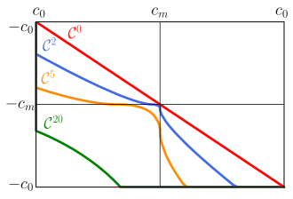
Figure 5: Theoretical curves $\mathcal{C}^{\,t}$ representing $\lambda^{-}$ as a function of $\lambda^{+}$ at a given time in the characteristic plane. The curves are plotted for $t=0$ ($\mathcal{C}^{\,0}$, in red), $t=2$ (blue), $t=5$ (orange) and $t=20>t_{\rm\scriptscriptstyle SW}(c_{m})$ (green). The corresponding initial distribution $\lambda^{\pm}(x,0)$ is schematically represented in the upper part of Fig. 2. We take here $c_{0}=1/\sqrt{2}$ and $c_{m}=\sqrt{2}$.

$\bullet$ The approach described in the present section makes it possible to determine the curve ${\cal C}^{\,t}$ representing, at time $t$, the profile in the unfolded characteristic plane. A sketch of ${\cal C}^{\,t}$ was given in Fig. 3(b), it is now precisely represented in Fig. (5) for several values of $t$, with also the initial curve ${\cal C}^{0}$.

Once $\lambda^{+}$ and $\lambda^{-}$ have been determined as functions of $x$ and $t$, the density and velocity profiles are obtained through Eqs. (8). One obtains an excellent description of the initial dispersionless stage of evolution of the pulse, as demonstrated by the very good agreement between theory and numerical simulations illustrated in Figs. 6 and 7. These figures, together with Fig. 8, compare at different times the theoretical density profile $\rho(x,t)$ with the one obtained by numerical integration of Eq. (2), taking the initial condition $u(x,0)=0$ and $\rho(x,0)$ given by (3) with $\rho_{0}=0.5$, $\rho_{m}=2$ and $x_{0}=20$.

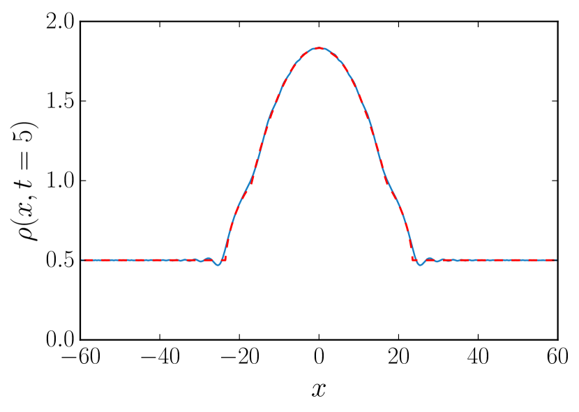
Figure 6: Comparison between theory and simulations for $t=5$. The red dashed line is extracted from the exact solution of the dispersionless system (9) (see the text), while the blue curve displays the numerical solution of Eq. (2) with the initial conditions $u(x,0)=0$ and $\rho(x,0)$ given by Eq. (3) taking $\rho_{0}=0.5$, $\rho_{1}=1.5$ (i.e., $\rho_{m}=2$) and $x_{0}=20$. The corresponding initial distributions $\lambda^{\pm}(x,0)$ are drawn schematically in Fig. 2(a) with here $c_{0}=\sqrt{\rho_{0}}=\sqrt{0.5}$ and $c_{m}=\sqrt{\rho_{m}}=\sqrt{2}$.

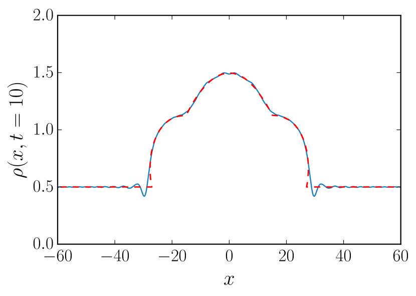
Figure 7: Same as Fig. 6 with here $t=10$. Notice that the dispersionless treatment leads to small regions of multivalued profile at both edges of the pulse.

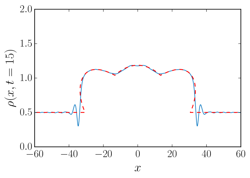
Figure 8: Same as Figs. 6 and 7 with here $t=15$. The multivaluedness of the theoretical profile is here obvious. It is associated to the formation of dispersive shocks at both edges of the pulse.

A similar agreement is obtained for the velocity profile $u(x,t)$. Note that for time $t=5$, some small diffractive contributions at the left and right boundary of the pulse are not accounted for by our dispersionless treatment (see Fig. 6). At larger time, the density profile at both ends of the pulse steepens and the amplitude of these oscillations accordingly increases. There exists a certain time, the wave breaking time $t_{\scriptscriptstyle\rm WB}$, at which nonlinear spreading leads to a gradient catastrophe; the dispersionless approximation subsequently predicts a nonphysical multivalued profile, as can be already seen in Fig. 7 and more clearly in Fig. 8. The time $t_{\scriptscriptstyle\rm WB}$ can be easily computed if the wave breaking occurs at the simple-wave edges of the pulse (see, e.g., LL-6 ) as it happens in our case, when the simple waves I and III break. These edges propagate with the “sound” velocity $c_{0}$ over a flat background and, at the wave breaking moment, the profile of $\lambda^{+}$ in region III (or $\lambda^{-}$ in region I) has a vertical tangent line in the limit $\lambda^{+}\to c_{0}$ ($\lambda^{-}\to-c_{0}$), that is $\partial x/\partial\lambda^{\pm}\to 0$ as $\lambda^{\pm}\to\pm c_{0}$. Then differentiation of the simple-wave solutions (39) or (40) gives at once

$$t_{\scriptscriptstyle\rm WB}=\frac{2}{3}\left|\frac{dW^{(3)}_{+}(-c_{0},\lambda^{+})}{d\lambda^{+}}\right|_{\lambda^{+}=c_{0}}$$ (45)

(for definiteness we consider the simple wave in the region III). Substitution of the expression for $W^{(3)}_{+}(-c_{0},\lambda^{+})$ in the above relation yields after simple calculations foot1

$$t_{\scriptscriptstyle\rm WB}=\frac{2}{3}\left|\frac{dw^{{\rm\scriptscriptstyle A}}}{d\lambda^{+}}\right|_{\lambda^{+}=c_{0}}.$$ (46)

The numerical value of $t_{\scriptscriptstyle\rm WB}$ is equal to $\simeq 6.3$ for our choice of initial condition, in excellent agreement with the onset of double valuedness of the solution of the Euler-Poisson. In dispersive nonlinear systems the wave breaking is regularized by formation of regions with large oscillations of density and flow velocity, whose extend increases with time. This situation is typical for the formation of dispersive shock waves, and requires a nonlinear treatment able to account for dispersive effects. Such an approach is introduced in the next section, but before turning to this aspect, we now compute an important characteristics time: the time $t_{\rm split}$ at which the initial bump has exactly split in two separated parts. For $t>t_{\rm split}$ a plateau of constant density $\rho_{0}$ develops between the two separated humps, as illustrated for instance in Fig. 1. One can see from Fig. 4 that $t_{\rm split}=t_{\rm\scriptscriptstyle SW}(c_{0})$ and can thus be computed from Eqs. (12) as

$$t_{\rm split}=\frac{W_{-}^{(2)}(-c_{0},c_{0})-W_{+}^{(2)}(-c_{0},c_{0})}{v_{+}(-c_{0},c_{0})-v_{-}(-c_{0},c_{0})}\;.$$ (47)

In the right hand side of the above equation one has $W_{\pm}^{(2)}=\partial_{\pm}\chi^{(2)}$ where it is legitimate to use the expression (35) since one is in the limiting case where $\lambda^{+}=-\lambda^{-}$. This yields at once

$$t_{\rm split}=\frac{x_{0}}{c_{0}}+\frac{1}{4\,c_{0}^{5/2}}\int_{c_{0}}^{c_{m}}\!\!\!\sqrt{r}\left(w^{\rm\scriptscriptstyle A}(r)-w^{\rm\scriptscriptstyle B}(r)\right)dr\;.$$ (48)

In the limit of a very small initial bump, $c_{m}$ is very close to $c_{0}$, and the second term of the right hand side of Eq. (48) is negligible. In this case a linear approach is valid: the two sub-parts of the bump move, one to the right, the other to the left, at velocities $\pm c_{0}$ and a time $t_{\rm split}\simeq x_{0}/c_{0}$ is needed for their complete separation. The second term of the right hand side of Eq. (48) describes the nonlinear correction to this result. For the initial profile (3) the expressions of $w^{\scriptscriptstyle\rm A}$ and $w^{\scriptscriptstyle\rm B}$ are given in Eq. (18) and one directly obtains from Eq. (48):

$$t_{\rm split}=\frac{x_{0}}{c_{0}}\Big{(}1+G(\rho_{1}/\rho_{0})\Big{)}\;,$$ (49)

where

$$G(X)=\frac{X}{4}\int_{0}^{1}\frac{\sqrt{1-u}}{(1+Xu)^{1/4}}du\;.$$ (50)

In the simulations, we took $x_{0}=20$, $c_{0}=\sqrt{0.5}$, $\rho_{1}/\rho_{0}=3$ and formula (49) then yields $t_{\rm split}\simeq 40.1$. Note that in this case the simple linear estimate would be $x_{0}/c_{0}\simeq 28.3$. The accuracy of the result (49) can be checked against numerical simulations, by plotting the numerically determined central density of the hump $\rho(x=0,t)$ as a function of time and checking that it just reaches the background value at $t=t_{\rm split}$. This is indeed the case: for the case we consider here $\rho(x=0,t=40.1)$ departs from $\rho_{0}$ by only 3 %.

For a small bump with $\rho_{1}\ll\rho_{0}$, the weak nonlinear correction to the linear result is obtained by evaluating the small $X$ behavior of the function $G$ in (50). This yields

$$t_{\rm split}\simeq\frac{x_{0}}{c_{0}}\left(1+\frac{1}{6}\,\frac{\rho_{1}}{\rho_{0}}-\frac{1}{60}\,\left(\frac{\rho_{1}}{\rho_{0}}\right)^{2}+\cdots\right)\;.$$ (51)

For the numerical values for which we performed the simulations, stopping expansion (51) at first order in $\rho_{1}/\rho_{0}$ yields $t_{\rm split}\simeq 42.4$. At next order one gets $t_{\rm split}\simeq 38.2$. These values are reasonable upper and lower bounds for the exact result. Of course, the expansion is more efficient for lower values of $\rho_{1}/\rho_{0}$: even for the relatively large value $\rho_{1}/\rho_{0}=1$, expansion (51) gives an estimate which is off the exact result (49) by only 0.3 %.

IV Whitham theory and the generalized hodograph method

In this section we first give a general presentation of Whitham modulational theory (Sec. IV.1) and then discuss specific features of its implementation for the case in which we are interested (Sec. IV.2).

IV.1 Periodic solutions and their modulations

The NLS equation (2) is equivalent to the system (6) which admits nonlinear periodic solutions that can be written in terms of four parameters $\lambda_{1}\leq\lambda_{2}\leq\lambda_{3}\leq\lambda_{4}$ in the form (see, e.g., Ref. kamch-2000 )

$$\begin{split}\rho(x,t)=&\tfrac{1}{4}(\lambda_{4}-\lambda_{3}-\lambda_{2}+\lambda_{1})^{2}+\\ &(\lambda_{4}-\lambda_{3})(\lambda_{2}-\lambda_{1})\times\\ &\mathrm{sn}^{2}\left(\sqrt{(\lambda_{4}-\lambda_{2})(\lambda_{3}-\lambda_{1})}\,(x-Vt),m\right)\;,\\ u(x,t)=&V-\frac{C}{\rho(x,t)}\;,\end{split}$$ (52)

where $\mathrm{sn}$ is the Jacobi elliptic sine function (see. e.g., Ref. AS ),

$$\begin{split}&V=\tfrac{1}{2}\sum_{i=1}^{4}\lambda_{i}\;,\quad m=\frac{(\lambda_{2}-\lambda_{1})(\lambda_{4}-\lambda_{3})}{(\lambda_{4}-\lambda_{2})(\lambda_{3}-\lambda_{1})}\;,\end{split}$$ (53)

and

$$\begin{split}C=&\tfrac{1}{8}(-\lambda_{1}-\lambda_{2}+\lambda_{3}+\lambda_{4})\times\\ &(-\lambda_{1}+\lambda_{2}-\lambda_{3}+\lambda_{4})\times(\lambda_{1}-\lambda_{2}-\lambda_{3}+\lambda_{4})\;.\end{split}$$ (54)

For constant $\lambda_{i}$’s, expressions (52), (53) and (54) correspond to an exact (single phase) solution of the NLS equation, periodic in time and space, where oscillations have the amplitude

$$a=(\lambda_{2}-\lambda_{1})(\lambda_{4}-\lambda_{3})\;,$$ (55)

and the spatial wavelength

$$L=\frac{2\,\mathrm{K}(m)}{\sqrt{(\lambda_{4}-\lambda_{2})(\lambda_{3}-\lambda_{1})}}\;.$$ (56)

In the limit $m\to 0$ ($\lambda_{1}=\lambda_{2}$ or $\lambda_{3}=\lambda_{4}$), $\mathrm{sn}(x,m)\to\sin(x)$ Eq. (52) describes a small amplitude sinusoidal wave oscillating around a constant background. In the other limiting case $m\to 1$ ($\lambda_{2}=\lambda_{3}$), $\mathrm{sn}(x,m)\to\tanh(x)$ and Eq. (52) describes a dark soliton (for which $L\to\infty$).

The great insight of Gurevich and Pitaevskii gp-73 has been to describe a dispersive shock wave as a slowly modulated nonlinear wave, of type (52), for which the $\lambda_{i}$’s are functions of $x$ and $t$ which vary weakly over one wavelength and one period. Their slow evolution is governed by the Whitham equations whitham-74 ; kamch-2000

$$\partial_{t}\lambda_{i}+v_{i}(\lambda_{1},\lambda_{2},\lambda_{3},\lambda_{4})\,\partial_{x}\lambda_{i}=0,\quad i=1,2,3,4.$$ (57)

Comparing with Eqs. (9) one sees that the $\lambda_{i}$’s are the Riemann invariants of the Whitham equations first found in Refs. fl86 ; pavlov87 . The $v_{i}$’s are the associated characteristic velocities; their explicit expressions can be obtained from the relation Gur92 ; kamch-2000

$$v_{i}=V-\frac{1}{2}\frac{L}{\partial_{i}L},\quad i=1,2,3,4\;,$$ (58)

where $\partial_{i}=\partial/\partial\lambda_{i}$. This yields

$$\begin{array}[]{l}\displaystyle{v_{1}=V-\frac{(\lambda_{4}-\lambda_{1})(\lambda_{2}-\lambda_{1})\mathrm{K}(m)}{(\lambda_{4}-\lambda_{1})\mathrm{K}(m)-(\lambda_{4}-\lambda_{2})\mathrm{E}(m)},}\\[14.22636pt] \displaystyle{v_{2}=V+\frac{(\lambda_{3}-\lambda_{2})(\lambda_{2}-\lambda_{1})\mathrm{K}(m)}{(\lambda_{3}-\lambda_{2})\mathrm{K}(m)-(\lambda_{3}-\lambda_{1})\mathrm{E}(m)},}\\[14.22636pt] \displaystyle{v_{3}=V-\frac{(\lambda_{4}-\lambda_{3})(\lambda_{3}-\lambda_{2})\mathrm{K}(m)}{(\lambda_{3}-\lambda_{2})\mathrm{K}(m)-(\lambda_{4}-\lambda_{2})\mathrm{E}(m)},}\\[14.22636pt] \displaystyle{v_{4}=V+\frac{(\lambda_{4}-\lambda_{3})(\lambda_{4}-\lambda_{1})\mathrm{K}(m)}{(\lambda_{4}-\lambda_{1})\mathrm{K}(m)-(\lambda_{3}-\lambda_{1})\mathrm{E}(m)},}\end{array}$$ (59)

where $m$ is given by Eq. (53) and $\mathrm{E}(m)$ is the complete elliptic integrals of the second kind.

In the soliton limit $m\to 1$ (i.e., $\lambda_{3}\to\lambda_{2}$), the Whitham velocities reduce to

$$\begin{split}&v_{1}=\tfrac{1}{2}(3\lambda_{1}+\lambda_{4}),\quad v_{2}=v_{3}=\tfrac{1}{2}(\lambda_{1}+2\lambda_{2}+\lambda_{4}),\\ &v_{4}=\tfrac{1}{2}(\lambda_{1}+3\lambda_{4}).\end{split}$$ (60)

In a similar way, in the small amplitude limit $m\to 0$ (i.e., $\lambda_{2}\to\lambda_{1}$), we obtain

$$\begin{split}&v_{1}=v_{2}=2\lambda_{1}+\frac{(\lambda_{4}-\lambda_{3})^{2}}{2(\lambda_{3}+\lambda_{4}-2\lambda_{1})},\\ &v_{3}=\tfrac{1}{2}(3\lambda_{3}+\lambda_{4}),\quad v_{4}=\tfrac{1}{2}(\lambda_{3}+3\lambda_{4}),\end{split}$$ (61)

and in another small amplitude limit ($m\to 0$ when $\lambda_{3}\to\lambda_{4}$), we have

$$\begin{split}&v_{1}=\tfrac{1}{2}(3\lambda_{1}+\lambda_{2}),\quad v_{2}=\tfrac{1}{2}(\lambda_{1}+3\lambda_{2}),\\ &v_{3}=v_{4}=2\lambda_{4}+\frac{(\lambda_{2}-\lambda_{1})^{2}}{2(\lambda_{1}+\lambda_{2}-2\lambda_{4})}.\end{split}$$ (62)

IV.2 Generalized hodograph method

In Sec. III we have provided a nondispersive description of the spreading and splitting of the initial pulse in two parts (one propagating to the left, and the other to the right). During this nonlinear process the leading wavefront steepens and leads to wave breaking. This occurs at a certain time $t_{\scriptscriptstyle\rm WB}$ after which the approach of Sec III predicts a nonphysical multivalued profile [see, e.g., Fig. 8], since it does not take into account dispersive effects. The process of dispersive regularization of the gradient catastrophe leads to the formation of a dispersive shock wave, as first predicted by Sagdeev in the context of collisionless plasma physics, see, e.g., Ref. Moi63 .

For the specific case we are interested in, the Gurevich-Pitaevskii approach which consists in using Whitham theory for describing the DSW as a slowly modulated nonlinear wave holds, but it is complicated by the fact that two of the four Riemann invariants vary in the shock region. As already explained in the introduction, we adapt here the method developed in Refs. Gur91 ; Gur92 ; Kry92 ; ek-93 for treating a similar situation for the Korteweg-de Vries equation. The general case of NLS dispersive shock with all four Riemann invariants varying was considered in Ref. ek-95 .

In all the following we concentrate our attention on the shock formed at the right edge of the pulse propagating to the right. Due to the symmetry of the problem the same treatment can be employed for the left pulse. The prediction of multivalued $\lambda^{+}$ resulting from the dispersionless approach of Sec. III suggests that after wave breaking of the simple-wave solution, the correct Whitham-Riemann invariant should be sought in a configuration such that $\lambda_{1}=\lambda^{-}=-c_{0}$, $\lambda_{2}=\lambda^{+}(x\to\infty)=c_{0}$ and $\lambda_{3}$ and $\lambda_{4}$ both depend on $x,t$. In this case the Whitham Eqs. (57) with $i=1,\,2$ are trivially satisfied, and for solving them for $i=3$ and 4, one introduces two functions $W_{i}(\lambda_{3},\lambda_{4})$ ($i=3$ or 4), exactly as we did in Sec. III with $W_{\pm}(\lambda^{-},\lambda^{+})$:

$$x-v_{i}(\lambda_{3},\lambda_{4})t=W_{i}(\lambda_{3},\lambda_{4}),\quad i=3,4\;.$$ (63)

For the sake of brevity we have denoted in the above equation $v_{i}(\lambda_{3},\lambda_{4})=v_{i}(\lambda_{1}=-c_{0},\lambda_{2}=c_{0},\lambda_{3},\lambda_{4})$ for $i\in\{3,4\}$; we will keep this notation henceforth.

Then, one can derive Tsarev equations for $W_{i}(\lambda_{3},\lambda_{4})$ [replacing the subscripts $+$ and $-$ by $4$ and $3$ in (13)] and one can show (see, e.g., Refs. Gur92 ; ek-95 ; wright ; tian ) that these are solved for $W_{i}$’s of the form

$$W_{i}=\left(1-\frac{L}{\partial_{i}L}\partial_{i}\right)\mathscr{W}=\mathscr{W}+2\,(v_{i}-V)\partial_{i}\mathscr{W}\;,$$ (64)

where $\mathscr{W}(\lambda_{3},\lambda_{4})$ is solution of the Euler-Poisson equation

$$\partial_{34}\mathscr{W}=\frac{\partial_{3}\mathscr{W}-\partial_{4}\mathscr{W}}{2(\lambda_{3}-\lambda_{4})}\;.$$ (65)

As was first understood in Ref. gkm-89 , after the wave breaking time, the development of the dispersive shock wave occurs in two steps. Initially (when $t$ is close to $t_{\scriptscriptstyle\rm WB}$), the DSW is connected at its left edge to the smooth profile coming from the time evolution of the right part of the initial profile of $\lambda^{+}$ (part A), which is gradually absorbed in the DSW. This process of absorption is complete at a time we denote as $t_{\scriptscriptstyle\rm A/B}$. Then, for $t>t_{\scriptscriptstyle\rm A/B}$, the DSW is connected to the smooth profile coming from the time evolution of part B of $\lambda^{+}$ (this is case “B”, “region B” of the $(x,t)$ plane). During the initial step (for $t<t_{\scriptscriptstyle\rm A/B}$), for a given time $t$, the highest value of the largest of the Riemann invariant is reached within the smooth part of the profile and keeps the constant value $c_{m}$. Then, in the subsequent time evolution, this highest value is reached within the DSW (or at its right boundary) where there exists a point where $\lambda_{4}$ takes its maximal value ($c_{m}$). We illustrate these two steps of development of the DSW in Fig. 9. We denote the region of the DSW where $\lambda_{4}$ is a decreasing function of $x$ as region A, the part where it increases as region B.

In region A of the $(x,t)$ plane, we denote by $\mathscr{W}^{\scriptscriptstyle\rm A}(\lambda_{3},\lambda_{4})$ the solution of the Euler-Poisson equation, in region B we denote it instead as $\mathscr{W}^{\scriptscriptstyle\rm B}(\lambda_{3},\lambda_{4})$. These two forms are joined by the line $\lambda_{4}=c_{m}$ where

$$\mathscr{W}^{\scriptscriptstyle\rm A}(\lambda_{3},c_{m})=\mathscr{W}^{\scriptscriptstyle\rm B}(\lambda_{3},c_{m})\;.$$ (66)

We denote the position where this matching condition is realized as $x_{m}(t)$, see Fig. 9(b). The corresponding boundary in the $(x,t)$ plane is represented as a green solid line in Fig. 10.

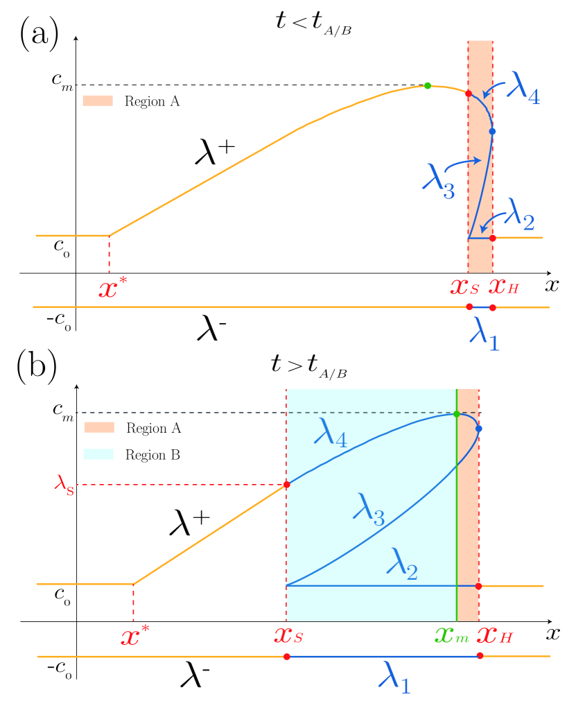
Figure 9: Schematic plots of the position dependence of the Riemann invariants inside (blue solid curves) and outside (yellow solid curves) the DSW (colored region). (a) For $t<t_{\scriptscriptstyle\rm A/B}$, the DSW is connected to the smooth profile coming from the time evolution of part A of the initial pulse. At $t=t_{\scriptscriptstyle\rm A/B}$, part A is completely absorbed by the DSW. Thus, for this time, the shock wave connects to the smooth profile exactly at $\lambda_{+}(x_{\scriptscriptstyle\rm S}(t),t)=c_{m}$. (b) For $t>t_{\scriptscriptstyle\rm A/B}$, the DSW is connected at its left edge at a point belonging to part B of the dispersionless profile. In this case the shock wave is divided in two regions A and B, separated by the green vertical line in the plot. The continuity along the separation line between the two regions (i.e., at $x=x_{m}(t)$) is ensured by Eq. (66).

Since the general solution of the Euler-Poisson equation with the appropriate boundary conditions and the construction of the resulting nonlinear pattern are quite involved, we shall first consider some particular—but useful—results which follow from general principles of the Whitham theory.

V Motion of the soliton edge of the shock

During the first stage of evolution of the DSW, its left (solitonic) edge is connected to the smooth dispersionless solution whose dynamics is described by formula (39), that is, we have here

$$x_{\scriptscriptstyle\rm S}-v_{+}(-c_{0},\lambda_{\scriptscriptstyle\rm S})\,t=W_{+}^{(3)}(-c_{0},\lambda_{\scriptscriptstyle\rm S}),$$ (67)

where $x_{\scriptscriptstyle\rm S}(t)$ is the position of the left edge of the DSW and $\lambda_{\scriptscriptstyle\rm S}(t)\equiv\lambda^{+}(x_{\scriptscriptstyle\rm S}(t),t)$. We recall that in all the following we focus on the DSW formed in the right part of the pulse. Hence the above equation concerns the right part of the nondispersive part of the profile. According to the terminology of section III, this corresponds to region III.

On the other hand, in vicinity of this boundary, the Whitham equations (57) with the limiting expressions (60) (where $\lambda_{2}=\lambda_{3}=c_{0}$) for the velocities $v_{i}$ are given by

$$\begin{split}&{\partial_{t}}\lambda_{3}+\frac{1}{2}\left(\lambda_{4}+c_{0}\right){\partial_{x}}\lambda_{3}=0,\\ &{\partial_{t}}\lambda_{4}+\frac{1}{2}\left(3\lambda_{4}-c_{0}\right){\partial_{x}}\lambda_{4}=0.\end{split}$$ (68)

For solving these equations one can perform a classical hodograph transform, that is, one assumes that $x$ and $t$ are functions of the independent variables $\lambda_{3}$ and $\lambda_{4}$: $t=t(\lambda_{3},\lambda_{4})$ and $x=x(\lambda_{3},\lambda_{4})$. We find from Eqs. (68) that these functions must satisfy the linear system

$$\begin{split}&\frac{\partial x}{\partial\lambda_{3}}-\frac{1}{2}\left(3\lambda_{4}-c_{0}\right)\frac{\partial t}{\partial\lambda_{3}}=0,\\ &\frac{\partial x}{\partial\lambda_{4}}-\frac{1}{2}\left(\lambda_{4}+c_{0}\right)\frac{\partial t}{\partial\lambda_{4}}=0.\end{split}$$

At the left edge of the DSW, the second equation reads

$$\frac{\partial x_{\scriptscriptstyle\rm S}}{\partial\lambda_{\scriptscriptstyle\rm S}}-\frac{1}{2}\left(\lambda_{\scriptscriptstyle\rm S}+c_{0}\right)\frac{\partial t}{\partial\lambda_{\scriptscriptstyle\rm S}}=0,$$ (69)

and this must be compatible with Eq. (67). Differentiation of Eq. (67) with respect to $\lambda_{\scriptscriptstyle\rm S}$ and elimination of $\partial x_{\scriptscriptstyle\rm S}/\partial\lambda_{\scriptscriptstyle\rm S}$ with the use of Eq. (69) yields a differential equation for the function $t(\lambda_{\scriptscriptstyle\rm S})\equiv t(c_{0},\lambda_{\scriptscriptstyle\rm S})$:

$$\left(\lambda_{\scriptscriptstyle\rm S}-c_{0}\right)\frac{dt}{d\lambda_{\scriptscriptstyle\rm S}}+\frac{3}{2}\,t=-\frac{dW_{+}^{(3)}(-c_{0},\lambda_{\scriptscriptstyle\rm S})}{d\lambda_{\scriptscriptstyle\rm S}}.$$ (70)

At the wave breaking time, $\lambda_{\scriptscriptstyle\rm S}=c_{0}$, this corresponds to the definition $t_{\rm\scriptscriptstyle WB}=t(c_{0})$ and Eq. (70) then yields

$$t_{\rm\scriptscriptstyle WB}=-\frac{2}{3}\left.\frac{dW_{+}^{(3)}(-c_{0},\lambda_{\scriptscriptstyle\rm S})}{d\lambda_{\scriptscriptstyle\rm S}}\right|_{\lambda_{\scriptscriptstyle\rm S}=c_{0}}\;,$$ (71)

in agreement with Eq. (46), what should be expected since at the wave breaking moment the DSW reduces to a point in the Whitham approximation. For the concrete case of our initial distribution we can get a simple explicit expression for $t_{\scriptscriptstyle\rm WB}$ which reads (see Eq. (46) and note foot1 ):

$$t_{\rm\scriptscriptstyle WB}=-\frac{2}{3}\left.\frac{dw^{\scriptscriptstyle\rm A}(\lambda_{\scriptscriptstyle\rm S})}{d\lambda_{\scriptscriptstyle\rm S}}\right|_{\lambda_{\scriptscriptstyle\rm S}=c_{0}}=\frac{2\,c_{0}\,x_{0}}{3\,\rho_{1}}\;,$$ (72)

where the right hand side is the form of the central formula corresponding to the initial profile (3). Taking $\rho_{0}=0.5$, $\rho_{m}=2$ and $x_{0}=20$, we find $t_{\rm\scriptscriptstyle WB}\simeq 6.3$, in excellent agreement with the numerical simulations.

The solution of Eq. (70) reads

$$\begin{split}t(\lambda_{\scriptscriptstyle\rm S})&=\frac{-1}{(\lambda_{\scriptscriptstyle\rm S}-c_{0})^{3/2}}\int_{c_{0}}^{\lambda_{\scriptscriptstyle\rm S}}\!\!\!\sqrt{r-c_{0}}\,\frac{dW_{+}^{(3)}(-c_{0},r)}{dr}\,dr\\ &=\frac{1}{2(\lambda_{\scriptscriptstyle\rm S}-c_{0})^{3/2}}\int_{c_{0}}^{\lambda_{\scriptscriptstyle\rm S}}\frac{W_{+}^{(3)}(-c_{0},r)}{\sqrt{r-c_{0}}}dr\\ &-\frac{W_{+}^{(3)}(-c_{0},\lambda_{\scriptscriptstyle\rm S})}{\lambda_{\scriptscriptstyle\rm S}-c_{0}}.\end{split}$$ (73)

Substituting this expression into (67), we obtain the function $x_{\scriptscriptstyle\rm S}(\lambda_{\scriptscriptstyle\rm S})\equiv x(c_{0},\lambda_{\scriptscriptstyle\rm S})$:

$$x_{\scriptscriptstyle\rm S}(\lambda_{\scriptscriptstyle\rm S})=\frac{1}{2}\left(3\lambda_{\scriptscriptstyle\rm S}-c_{0}\right)\,t(\lambda_{\scriptscriptstyle\rm S})+W_{+}^{(3)}(-c_{0},\lambda_{\scriptscriptstyle\rm S}).$$ (74)

The two formulas (73) and (74) define in an implicit way the law of motion $x=x_{\scriptscriptstyle\rm S}(t)$ of the soliton edge of the DSW.

The above expressions are correct as long as the soliton edge is located inside region A of the DSW, that is, up to the moment $t_{\scriptscriptstyle\rm A/B}=t(c_{m})$. From (73) one obtains the explicit expression

$$t_{\scriptscriptstyle\rm A/B}=\frac{-1}{(c_{m}-c_{0})^{3/2}}\int_{c_{0}}^{c_{m}}\!\!\!\sqrt{r-c_{0}}\,\frac{dW_{+}^{(3)}(-c_{0},r)}{dr}\,dr.$$ (75)

In the case we consider this yields $t_{\scriptscriptstyle\rm A/B}=25.9$. For time larger than $t_{\scriptscriptstyle\rm A/B}$ the soliton edge connects with region B of the dispersionless profile which corresponds to region II_r, see Fig. 4. Concretely, for a time $t>t_{\scriptscriptstyle\rm A/B}$, instead of Eq. (70) we have to solve the differential equation

$$\left(\lambda_{\scriptscriptstyle\rm S}-c_{0}\right)\frac{dt}{d\lambda_{\scriptscriptstyle\rm S}}+\frac{3}{2}\,t=-\frac{dW_{+}^{(2)}(-c_{0},\lambda_{\scriptscriptstyle\rm S})}{d\lambda_{\scriptscriptstyle\rm S}}.$$ (76)

with the initial condition $t(c_{m})=t_{\scriptscriptstyle\rm A/B}$. The solution of Eq. (76) reads

$$\begin{split}t(\lambda_{\scriptscriptstyle\rm S})=&\frac{-1}{(\lambda_{\scriptscriptstyle\rm S}-c_{0})^{3/2}}\Bigg{(}\int_{c_{m}}^{\lambda_{\scriptscriptstyle\rm S}}\!\!\sqrt{r-c_{0}}\,\frac{dW_{+}^{(2)}(-c_{0},r)}{dr}dr\\ &+\int_{c_{0}}^{c_{m}}\sqrt{r-c_{0}}\,\frac{dW_{+}^{(3)}(-c_{0},r)}{dr}dr\Bigg{)},\end{split}$$ (77)

and $x_{\scriptscriptstyle\rm S}(\lambda_{\scriptscriptstyle\rm S})$ is determined by Eq. (41):

$$x_{\scriptscriptstyle\rm S}(\lambda_{\scriptscriptstyle\rm S})=\frac{1}{2}\left(3\lambda_{\scriptscriptstyle\rm S}-c_{0}\right)\,t(\lambda_{\scriptscriptstyle\rm S})+W_{+}^{(2)}(-c_{0},\lambda_{\scriptscriptstyle\rm S}).$$ (78)

At asymptotically large time $t\to\infty$ one is in stage B of evolution of the DSW with furthermore $\lambda_{\scriptscriptstyle\rm S}\to c_{0}$. In this case the upper limit of integration in the first integral of formula (77) can be put equal to $c_{0}$. Thus, we get in this limit

$$t(\lambda_{\scriptscriptstyle\rm S})\simeq\frac{\cal A}{(\lambda_{\scriptscriptstyle\rm S}-c_{0})^{3/2}},$$ (79)

where the expression for the constant ${\cal A}$ is

$$\begin{split}\cal A=&-\Bigg{(}\int_{c_{m}}^{c_{0}}\sqrt{r-c_{0}}\,\frac{dW_{+}^{(2)}(-c_{0},r)}{dr}dr\\ &+\int_{c_{0}}^{c_{m}}\sqrt{r-c_{0}}\,\frac{dW_{+}^{(3)}(-c_{0},r)}{dr}dr\Bigg{)}.\end{split}$$ (80)

Consequently one obtains the asymptotic expressions

$$\lambda_{\scriptscriptstyle\rm S}(t)=c_{0}+\left(\frac{\cal A}{t}\right)^{2/3}\;,\quad x_{\scriptscriptstyle\rm S}(t)=c_{0}\,t+\frac{3{\cal A}^{2/3}}{2}\,t^{1/3}\;.$$ (81)

We denote the position of the rear point of the simple wave as $x^{*}(t)$, see Fig. 9. It is clear from Fig. 4 that $x^{*}=0$ at time $t=t_{\scriptscriptstyle\rm SW}(c_{0})$, i.e., just when region 2 disappears, whereafter the dispersionless approach of Sec. III predicts a profile with only simple waves and plateau regions. The rear edge of the simple wave then propagates over a flat background at constant velocity $c_{0}$; one thus has

$$x^{*}(t)=c_{0}\left[t-t_{\scriptscriptstyle\rm SW}(c_{0})\right]\;.$$ (82)

Asymptotically (i.e., at time much larger than $t_{\scriptscriptstyle\rm SW}(c_{0})$) one has $x^{*}(t)\simeq c_{0}t$ and, in the simple wave profile between $x^{*}(t)$ and $x_{\scriptscriptstyle\rm S}(t)$, $\lambda^{+}$ depends on the self-similar variable $(x-x^{*}(t))/t$ while $\lambda^{-}$ is constant. Then Eqs. (9) readily yield

$$\begin{cases}\lambda^{+}=c_{0}+\frac{2}{3}\frac{\displaystyle x-x^{*}(t)}{\displaystyle t},\\ \lambda^{-}=-c_{0},\end{cases}\mbox{for}\;x\in[x^{*}(t),x_{\scriptscriptstyle\rm S}(t)]\;.$$ (83)

Eqs. (8) then yield the explicit expression of $\rho$ in this region (which was roughly described in the end of Sec. II as having a “quasi-triangular shape”), and using (81) one obtains

$$\int_{x^{*}(t)}^{x_{\scriptscriptstyle\rm S}(t)}\left(\sqrt{\rho(x,t)}-c_{0}\right)^{1/2}dx=\frac{1}{\sqrt{2}}\,{\cal A}\;.$$ (84)

The asymptotic situation at the rear of the DSW is reminiscent of what occurs in the theory of weak dissipative shocks where (i) a nonlinear pattern of triangular shape may also appear at the rear edge of a (viscous) shock, (ii) the details of the initial distribution are lost at large time (as in the present case) and (iii) a conserved quantity of the type (84) also exists. Hence the above results provide, for a conservative system, the counterpart of the weak viscous shock theory (presented for instance in Ref. whitham-74 ). Note, however, that the boundary conditions at the large amplitude edge of the shock are different depending on whether one considers a dissipative or a conservative system, and that the corresponding velocity and conserved quantity are accordingly also different. Note also that equivalent relations for the behavior of a rarefaction wave in the rear of a dispersive shock in the similar situation for the Korteweg-de Vries equation has been obtained in Ref. Iso18 .

Formulas (81) and (84) are important because they provide an indirect evidence making it possible to assert if a given experiment has indeed reached to the point where a bona fide dispersive shock wave should be expected.

We now give, in the next section, the explicit theoretical description of the whole region of the dispersive shock.

VI Solution in the shock region

In this section we turn to the general solution of the Whitham equations given by the formulas of Sec. IV.2. Our task is to express the functions $W_{3}$ and $W_{4}$ in terms of the initial distribution of the light pulse. As was indicated above, one needs to distinguish two regions, A and B, in which $\mathscr{W}$ takes different values.

VI.1 Solution in region A

In region A one can straightforwardly adapt the procedure explained in Ref. Gur92 . One imposes the matching of the left edge of the DSW with the dispersionless solution (see Sec. III.2): just at $x=x_{\scriptscriptstyle\rm S}(t)$, we have $\lambda_{4}=\lambda^{+}$, $\lambda_{3}=\lambda_{2}=c_{0}$, $\lambda_{1}=-c_{0}$ (see Fig. 9) and Eq. (60) yields $v_{4}(\lambda_{3},\lambda_{4})=(3\,\lambda_{4}-c_{0})/2=v_{+}(-c_{0},\lambda^{+})$. Then, at this point, the conditions (39) and (63) with $i=4$ are simultaneously satisfied which implies

$$W^{\scriptscriptstyle\rm A}_{4}(\lambda_{3}=c_{0},\lambda_{4}=\lambda^{+})=W_{+}^{(3)}(-c_{0},\lambda^{+})\;,$$ (85)

where $W_{+}^{(3)}$ is the form of $W_{+}$ corresponding to region 3. Note that, here, the first argument of the function $W_{+}^{(3)}$ is $\lambda^{-}=-c_{0}$ for all time. Indeed, the boundary condition (85) corresponds to the matching in physical space at $x_{\scriptscriptstyle\rm S}(t)$. When the DSW starts to form at time $t_{\scriptscriptstyle\rm WB}$, the edge $x_{\scriptscriptstyle\rm S}(t_{\scriptscriptstyle\rm WB})$ lies on the characteristic issued from $x_{0}$ [$x_{0}$ defines the initial extend of the pulse, see. Eq. (3)]. The Riemann invariant $\lambda^{-}$ is constant and equal to $-c_{0}$ along this characteristic, cf. Fig. 4. Then, because the characteristics of $\lambda^{-}$ in the dispersionless region close to $x_{\scriptscriptstyle\rm S}$ are oriented to the left whereas $x_{\scriptscriptstyle\rm S}$ moves to the right, it is clear that $\lambda^{-}(x_{\scriptscriptstyle\rm S}(t),t)=-c_{0}$ for $t\geq t_{\scriptscriptstyle\rm WB}$.

In terms of $\mathscr{W}$ the relation (85) corresponds to the equation

$$\mathscr{W}^{\scriptscriptstyle\rm A}(c_{0},\lambda_{4})+2\,(\lambda_{4}-c_{0})\partial_{4}\mathscr{W}^{\scriptscriptstyle\rm A}(c_{0},\lambda_{4})=W_{+}^{(3)}(-c_{0},\lambda_{4})\;,$$ (86)

whose solution is

$$\mathscr{W}^{\scriptscriptstyle\rm A}\left(c_{0},\lambda_{4}\right)=\frac{1}{2\,\sqrt{\lambda_{4}-c_{0}}}\int_{c_{0}}^{\lambda_{4}}\frac{W^{(3)}_{+}(-c_{0},r)\,dr}{\sqrt{r-c_{0}}}\;.$$ (87)

This will serve as a boundary condition for the Euler-Poisson equation (65) whose general solution has been given by Eisenhart Eis18 in the form

$$\begin{split}\mathscr{W}^{\scriptscriptstyle\rm A}(\lambda_{3},\lambda_{4})=&\int_{c_{0}}^{\lambda_{3}}\frac{\psi^{\scriptscriptstyle\rm A}(\mu)\,d\mu}{\sqrt{\lambda_{3}-\mu}\sqrt{\lambda_{4}-\mu}}+\\ &\int_{c_{0}}^{\lambda_{4}}\frac{\varphi^{\scriptscriptstyle\rm A}(\mu)\,d\mu}{\sqrt{|\lambda_{3}-\mu|}\sqrt{\lambda_{4}-\mu}}\;,\end{split}$$ (88)

where $\varphi^{\scriptscriptstyle\rm A}(\mu)$ and $\psi^{\scriptscriptstyle\rm A}(\mu)$ are arbitrary functions to be determined from the appropriate boundary conditions. By taking $\lambda_{3}=c_{0}$ in this expression one sees that $\varphi^{\scriptscriptstyle\rm A}(\mu)/\sqrt{\mu-c_{0}}$ is the Abel transform of $\mathscr{W}^{\scriptscriptstyle\rm A}(c_{0},\lambda_{4})$. Using the inverse transformation Ark05 and expression (87) one can show that

$$\varphi^{\scriptscriptstyle\rm A}(\mu)=\frac{1}{2\pi\,\sqrt{\mu-c_{0}}}\int_{c_{0}}^{\mu}\frac{W^{(3)}_{+}(-c_{0},r)\,dr}{\sqrt{\mu-r}}\;,$$ (89)

where we recall that $W^{(3)}_{+}=\partial_{+}\chi^{(3)}$. In order to determine the other unknown function $\psi^{\scriptscriptstyle\rm A}$, one considers the right boundary of the DSW where $\lambda_{3}$ and $\lambda_{4}$ are asymptotically close to each other. One can show (see, e.g., an equivalent reasoning in Ref. Iso18 ) that in order to avoid divergence of $\mathscr{W}^{\scriptscriptstyle\rm A}(\lambda_{3},\lambda_{4}=\lambda_{3})$, one needs to impose $\psi^{\scriptscriptstyle\rm A}(\lambda)=-\varphi^{\scriptscriptstyle\rm A}(\lambda)$. The final form of the Eisenhart solution in region A thus reads

$$\mathscr{W}^{\scriptscriptstyle\rm A}(\lambda_{3},\lambda_{4})=\int_{\lambda_{3}}^{\lambda_{4}}\frac{\varphi^{\scriptscriptstyle\rm A}(\mu)\,d\mu}{\sqrt{\mu-\lambda_{3}}\sqrt{\lambda_{4}-\mu}}\;,$$ (90)

where $\varphi^{\scriptscriptstyle\rm A}$ is given by formula (89).

VI.2 Solution in region B

One looks for a solution of the Euler-Poisson equation in region B in the form

$$\mathscr{W}^{\scriptscriptstyle\rm B}(\lambda_{3},\lambda_{4})=\mathscr{W}^{\scriptscriptstyle\rm A}(\lambda_{3},\lambda_{4})+\int_{\lambda_{4}}^{c_{m}}\!\!\!\frac{\varphi^{\scriptscriptstyle\rm B}(\mu)\,d\mu}{\sqrt{\mu-\lambda_{3}}\sqrt{\mu-\lambda_{4}}},$$ (91)

where $c_{m}$, the maximum value for $\lambda_{4}$. The above expression ensures that $\mathscr{W}^{\scriptscriptstyle\rm B}$, (i) being the sum of two solutions of the Euler-Poisson equation, is also a solution of this equation and (ii) verifies the boundary condition (66) since the second term of the right-hand side of (91) vanishes when $\lambda_{4}=c_{m}$.

At the left boundary of the DSW, $\mathscr{W}^{\scriptscriptstyle\rm B}(c_{0},\lambda_{4})$ verifies an equation similar to (86):

$$\mathscr{W}^{\scriptscriptstyle\rm B}(c_{0},\lambda_{4})+2\,(\lambda_{4}-c_{0})\partial_{4}\mathscr{W}^{\scriptscriptstyle\rm B}(c_{0},\lambda_{4})=W_{+}^{(2)}(-c_{0},\lambda_{4})\;,$$ (92)

The solution with the appropriate integration constant reads

$$\begin{split}\mathscr{W}^{\scriptscriptstyle\rm B}(r_{1},0)&=\frac{1}{2\,\sqrt{\lambda_{4}-c_{0}}}\int_{\lambda_{4}}^{c_{m}}\frac{W^{(2)}_{+}(-c_{0},r)}{\sqrt{r-c_{0}}}dr\\ &+\frac{1}{2\,\sqrt{\lambda_{4}-c_{0}}}\int_{c_{0}}^{c_{m}}\frac{W^{(3)}_{+}(-c_{0},r)}{\sqrt{r-c_{0}}}dr\;,\end{split}$$ (93)

where $W^{(2)}_{+}$ is the form of $W_{+}$ corresponding to region 2. The same procedure as the one previously used for the part A of the DSW leads here to

$$\varphi^{\scriptscriptstyle\rm B}(\mu)=\frac{1}{2\pi\,\sqrt{\mu-c_{0}}}\int_{\mu}^{c_{m}}\frac{W^{(3)}_{+}(-c_{0},r)-W^{(2)}_{+}(-c_{0},r)}{\sqrt{\mu-r}}dr\;.$$ (94)

Eqs. (91) and (94) give the solution of the Euler-Poisson equation in region B.

VI.3 Characteristics of the DSW at its edges

It is important to determine the boundaries $x_{\scriptscriptstyle\rm S}(t)$ and $x_{\scriptscriptstyle\rm H}(t)$ of the DSW, as well as the values of the Riemann invariants $\lambda_{3}$ and $\lambda_{4}$ at these points. The law of motion of the soliton edge was already found in Sec. V and it is instructive to show how this result can be obtained from the general solution.

At the soliton edge we have $\lambda_{2}=\lambda_{3}=c_{0}$ and $\lambda_{4}=\lambda_{\scriptscriptstyle\rm S}(t)$. The corresponding Whitham velocities are $v_{3}=(\lambda_{\scriptscriptstyle\rm S}+c_{0})/2$ and $v_{4}=(3\lambda_{\scriptscriptstyle\rm S}-c_{0})/2$ [see Eqs. (60)], and the two equations (63) read

$$\begin{split}x_{\scriptscriptstyle\rm S}-\frac{1}{2}\,(3\lambda_{\scriptscriptstyle\rm S}-c_{0})t=W_{4}^{\alpha}(c_{0},\lambda_{\scriptscriptstyle\rm S})&=W_{+}^{(n)}(-c_{0},\lambda_{\scriptscriptstyle\rm S}),\\ x_{\scriptscriptstyle\rm S}-\frac{1}{2}\,(\lambda_{\scriptscriptstyle\rm S}+c_{0})t=W_{3}^{\alpha}(c_{0},\lambda_{\scriptscriptstyle\rm S})&=\mathscr{W}^{\alpha}(c_{0},\lambda_{\scriptscriptstyle\rm S}),\end{split}$$ (95)

where, in order to have formulas applying to both stages of evolution of the DSW, one has introduced dummy indices $\alpha$ and $n$ with $\alpha=$ A or B and $n=3$ or 2, respectively. This gives at once

$$\begin{split}&t(\lambda_{\scriptscriptstyle\rm S})=\frac{1}{\lambda_{\scriptscriptstyle\rm S}-c_{0}}\left[\mathscr{W}^{\alpha}(c_{0},\lambda_{\scriptscriptstyle\rm S})-W_{+}^{(n)}(-c_{0},\lambda_{\scriptscriptstyle\rm S})\right],\\ &x_{\scriptscriptstyle\rm S}(\lambda_{\scriptscriptstyle\rm S})=c_{0}\,t+\frac{1}{2}\left[3\mathscr{W}^{\alpha}(c_{0},\lambda_{\scriptscriptstyle\rm S})-W_{+}^{(n)}(-c_{0},\lambda_{\scriptscriptstyle\rm S})\right].\end{split}$$ (96)

Let us consider the stage A for instance. Eq. (87) yields

$$\mathscr{W}^{A}\left(c_{0},\lambda_{\scriptscriptstyle\rm S}\right)=\frac{1}{2\,\sqrt{\lambda_{\scriptscriptstyle\rm S}-c_{0}}}\int_{c_{0}}^{\lambda_{\scriptscriptstyle\rm S}}\frac{W^{(3)}_{+}(-c_{0},r)\,dr}{\sqrt{r-c_{0}}},$$

which, inserted into Eqs. (96) gives immediately the results (73) and (74).

Fig. 10 shows the time evolution of $x_{\scriptscriptstyle\rm S}(t)$. The black curve is calculated from Eqs. (96), while the red dashed line corresponds to the asymptotic behavior of $x_{\scriptscriptstyle\rm S}$, given by Eq. (81). The green points are extracted from simulations and exhibit a very good agreement with the theory.

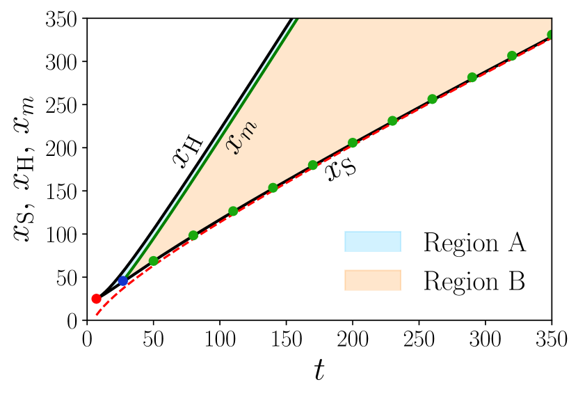
Figure 10: Black solid curves: time evolution of $x_{\scriptscriptstyle\rm S}(t)$ and $x_{\scriptscriptstyle\rm H}(t)$ calculated from Eqs. (96) and (99). Green solid curve: time evolution of $x_{m}(t)$, for which $\lambda_{4}(x_{m}(t),t)=c_{m}$, which marks the separation between regions A and B. Red dashed line: asymptotic behavior of $x_{\scriptscriptstyle\rm S}(t)$, from Eq. (81). The green points indicate the position $x_{\scriptscriptstyle\rm S}(t)$ extracted from simulations, for an initial condition (3) with $\rho_{0}=0.5$, $\rho_{m}=2$ and $x_{0}=20$. The red dot marks the birth of the DSW (at time $t_{\scriptscriptstyle\rm WB}\simeq 6.3$), while the blue one initiates region B (at time $t_{\scriptscriptstyle\rm A/B}\simeq 25.9$).

The same excellent agreement is obtained for the time evolution of $\lambda_{\scriptscriptstyle\rm S}$, as shown in Fig. 11.

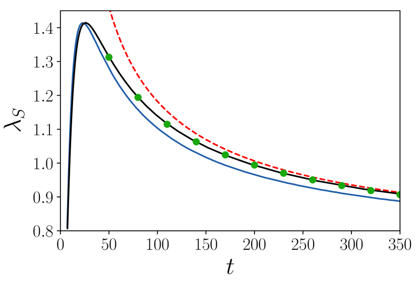
Figure 11: Black solid curve: time evolution of $\lambda_{\scriptscriptstyle\rm S}(t)$ from Eq. (96), or equivalently from Eqs. (73) and then (77). Red dashed line: asymptotic behavior, from Eq. (81). The green points are extracted from simulations for different times, for the initial profile (3) with $\rho_{0}=0.5$, $\rho_{m}=2$ and $x_{0}=20$. The blue solid curve is an approximation obtained by schematically describing the initial splitting by assuming $\lambda^{-}\simeq\text{cst}$ for all $t$’s during the evolution of the right pulse (see the text).

We demonstrated in Sec. III the accuracy of the Riemann method for describing the spreading and splitting of the initial pulse into two parts. The matching between the left edge of the DSW and the dispersionless profile at the point of coordinates $\left(x_{\scriptscriptstyle\rm S},\lambda_{\scriptscriptstyle\rm S}\right)$ is given in Eq. (67). Since the splitting occurs rapidly, a simpler approach would be to make the approximation $\lambda^{-}(x,t)=-c_{0}=\text{const}$ for the dispersionless right part of the profile. In this case, the Riemann equation (9) for $\lambda^{+}$ reduces to

$$\frac{\partial\lambda^{+}}{\partial t}+\left(\frac{3}{2}\lambda^{+}-\frac{1}{2}c_{0}\right)\frac{\partial\lambda^{+}}{\partial x}=0.$$ (97)

This equation can be solved by the method of characteristics which yields the implicit solution for $\lambda^{+}(x,t)$:

$$x-\left(\frac{3}{2}\lambda^{+}-\frac{1}{2}c_{0}\right)\,t=w^{\scriptscriptstyle\rm A/B}(\lambda^{+})\;,$$ (98)

where $w^{\scriptscriptstyle\rm A/B}$ are the the inverse functions of the initial $\lambda^{+}(x)$ profile in parts A and B [in our case their explicit expressions are given in Eqs. (18)].

Within this approximation the DSW is described through $\mathscr{W}$ by the same equations (89), (90), (91) and (94) as before, replacing $W_{+}^{(3/2)}(-c_{0},r)$ by $w^{\scriptscriptstyle\rm A/B}(r)$ everywhere. $\lambda_{\scriptscriptstyle\rm S}$ computed using this approximation is represented in Fig. 11 as a function of $t$ (blue solid line) where it is also compared with the results obtained using the full Riemann method (black solid line) and the results extracted from numerical simulations (green dots). As we can see, an accurate description of the spreading and splitting stage is important since the blue curve does not precisely agree with the results of the simulations, mainly at large times. However, this approximation gives a correct description of the initial formation of the DSW: this is discussed in note foot1 where it is argued that, close to the wave breaking time, the approximation $W_{+}^{(3)}(-c_{0},r)\simeq w^{\scriptscriptstyle\rm A}(r)$ is very accurate.

Let us now turn to the determination of the location $x_{\scriptscriptstyle\rm H}(t)$ of the small-amplitude, harmonic boundary of the DSW, and of the common value $\lambda_{\scriptscriptstyle\rm H}(t)$ of $\lambda_{3}$ and $\lambda_{4}$ at this point (see Fig. 9). In the typical situation the left boundary is located in region A. In this case the equations (63) for $i=3$ and 4 are equivalent and read

$$x_{\scriptscriptstyle\rm H}-v_{\scriptscriptstyle\rm H}\cdot t=W_{i}^{\scriptscriptstyle\rm A}(\lambda_{\scriptscriptstyle\rm H},\lambda_{\scriptscriptstyle\rm H})\;,\quad i=3\;\mbox{or}\;4\;,$$ (99)

where $v_{\scriptscriptstyle\rm H}=v_{i}(\lambda_{\scriptscriptstyle\rm H},\lambda_{\scriptscriptstyle\rm H})=2\,\lambda_{\scriptscriptstyle\rm H}-c_{0}^{2}/\lambda_{\scriptscriptstyle\rm H}$ [cf. Eqs. (62)]. An equation for $\lambda_{\scriptscriptstyle\rm H}$ alone is obtained by demanding that the velocity $dx_{\scriptscriptstyle\rm H}/dt$ of the left boundary is equal to the common value $v_{\scriptscriptstyle\rm H}$ of $v_{3}$ and $v_{4}$. The differentiation of Eq. (99) with respect to time then yields

$$t=-\frac{1}{{d}v_{\scriptscriptstyle\rm H}/{d}\lambda_{\scriptscriptstyle\rm H}}\,\frac{{d}W_{4}^{\scriptscriptstyle\rm A}(\lambda_{\scriptscriptstyle\rm H},\lambda_{\scriptscriptstyle\rm H})}{{d}\lambda_{\scriptscriptstyle\rm H}}\;.$$ (100)

Note that the relation $dx_{\scriptscriptstyle\rm H}/{d}t=v_{\scriptscriptstyle\rm H}$ is a consequence of the general statement that the small amplitude edge of the DSW propagates with the group velocity corresponding to the wave number determined by the solution of the Whitham equations. Indeed, the NLS group velocity of a linear wave with wave-vector $k$ moving over a background $\rho_{0}=c_{0}^{2}$ is the group velocity of the so called Bogoliubov waves:

$$v_{g}(k)=\frac{k^{2}/2+c_{0}^{2}}{\sqrt{k^{2}/4+c_{0}^{2}}},$$ (101)

and here $k=2\pi/L=2\sqrt{\lambda_{\scriptscriptstyle\rm H}^{2}-c_{0}^{2}}$ [where $L$ is computed from Eq. (56)]. This yields $v_{g}=2\,\lambda_{\scriptscriptstyle\rm H}-c_{0}^{2}/\lambda_{\scriptscriptstyle\rm H}=v_{\scriptscriptstyle\rm H}$, as it should. This property of the small-amplitude edge is especially important in the theory of DSWs for non-integrable equations (see, e.g., Refs. El05 ; Kam18 ).

The value of $W_{4}^{\scriptscriptstyle\rm A}(\lambda_{\scriptscriptstyle\rm H},\lambda_{\scriptscriptstyle\rm H})$ in Eq. (99) is computed through (63) and (90). One gets

$$W_{4}^{\scriptscriptstyle\rm A}(\lambda_{\scriptscriptstyle\rm H},\lambda_{\scriptscriptstyle\rm H})=\pi\,\varphi^{\scriptscriptstyle\rm A}(\lambda_{\scriptscriptstyle\rm H})+\pi\,\left(\lambda_{\scriptscriptstyle\rm H}-\frac{c_{0}^{2}}{\lambda_{\scriptscriptstyle\rm H}}\right)\frac{d\varphi^{\scriptscriptstyle\rm A}}{d\mu}(\lambda_{\scriptscriptstyle\rm H})\;,$$ (102)

and

$$\begin{split}\frac{{d}W_{4}^{\scriptscriptstyle\rm A}(\lambda_{\scriptscriptstyle\rm H},\lambda_{\scriptscriptstyle\rm H})}{d\lambda_{\scriptscriptstyle\rm H}}&=\pi\left(2+\frac{c_{0}^{2}}{\lambda_{\scriptscriptstyle\rm H}^{2}}\right)\frac{d\varphi^{\scriptscriptstyle\rm A}}{d\mu}(\lambda_{\scriptscriptstyle\rm H})\\ &+\pi\,\left(\lambda_{\scriptscriptstyle\rm H}-\frac{c_{0}^{2}}{\lambda_{\scriptscriptstyle\rm H}}\right)\frac{d^{2}\varphi^{\scriptscriptstyle\rm A}}{d\mu^{2}}(\lambda_{\scriptscriptstyle\rm H})\;,\end{split}$$ (103)

where $\varphi^{\scriptscriptstyle\rm A}$ is given by Eq. (89). Once expression (103) has been used to obtain $\lambda_{\scriptscriptstyle\rm H}(t)$ by solving Eq. (100), the position $x_{\scriptscriptstyle\rm H}(t)$ of the harmonic edge of the DSW is determined by (99). The time evolution of $x_{\scriptscriptstyle\rm H}(t)$ is displayed in Fig. 10.

The position of the point $x_{m}(t)$ where $\lambda_{4}=c_{m}$ (cf. Fig. 9) can be obtained from Eqs. (63). First, for a given time $t$, one needs to find the corresponding value $\lambda_{3}$, solution of the following equation

$$t=\frac{W_{3}(\lambda_{3},c_{m})-W_{4}(\lambda_{3},c_{m})}{v_{4}(\lambda_{3},c_{m})-v_{3}(\lambda_{3},c_{m})}.$$ (104)

Note that in the above we did not write the superscript A or B, because this formula equally holds in both cases since it is to be determined at the boundary between the two regions A and B of the DSW, cf. Eq. (66) and Fig. 9. Then, $x_{m}(t)$ is determined using any one of the Eqs. (63). The result is shown in Fig. 10, where the curve $x_{m}(t)$ represents the position of the boundary between the two regions A and B at time $t$.

VI.4 The global picture

We now compare the results of the Whitham approach with the numerical solution of the NLS equation (2) for the initial profile (3).

The DSW is described by Whitham method as explained in Secs. IV.1 and IV.2. For this purpose one needs to determine $\lambda_{3}$ and $\lambda_{4}$ as functions of $x$ and $t$ (whereas $\lambda_{1}=-c_{0}$ and $\lambda_{2}=c_{0}$). This is performed as follows:

• First, we pick up a given $\lambda_{4}\in[c_{0},\lambda_{\scriptscriptstyle\rm S}]$, where $\lambda_{\scriptscriptstyle\rm S}$ is the value of $\lambda_{4}$ at the soliton edge, the point where the DSW is connected to the rarefaction wave (it has been explained in Secs. V and VI.3 how to compute it).

• Second, at fixed $t$ and $\lambda_{4}$, we find the corresponding value $\lambda_{3}$ as a solution of the difference of equations (63),

  $$\left(v_{4}-v_{3}\right)\cdot t=W_{3}(\lambda_{3},\lambda_{4})-W_{4}(\lambda_{3},\lambda_{4})\,,$$ (105)

  where $W_{3}$ and $W_{4}$ are computed from Eq. (64), with a superscript A or B, as appropriate.

• Last, the corresponding value of $x$ is determined by $x=W_{3}+v_{3}t$ (or equivalently $x=W_{4}+v_{4}t$).

This procedure gives, for each $\lambda_{4}\in[c_{0},\lambda_{\scriptscriptstyle\rm S}]$ and $t$, the value of $\lambda_{3}$ and $x$. In practice, it makes it possible to associate with each $(x,t)$ a couple $(\lambda_{3},\lambda_{4})$. The results confirm the schematic behavior depicted in Fig. 9.

The knowledge of $\lambda_{3}(x,t)$ and $\lambda_{4}(x,t)$ completes our study and enable us to determine, for each time $t>t_{\rm\scriptscriptstyle WB}$, $\rho(x,t)$ and $u(x,t)$ as given by the Whitham approach, for all $x\in\mathbb{R}^{+}$. Denoting as ${x}^{*}(t)$ the left boundary of the hump (remember that we concentrate on the right part of the light intensity profile, see Fig. 9):

• In the two regions $x\geq x_{\scriptscriptstyle\rm H}(t)$ and $0\leq x\leq{x}^{*}(t)$, we have $u(x,t)=0$ and $\rho(x,t)=\rho_{0}$.

• In the dispersionless region $[{x}^{*}(t),x_{\scriptscriptstyle\rm S}(t)]$, $u(x,t)$ and $\rho(x,t)$ are computed from (7) in terms of $\lambda^{+}$ and $\lambda^{-}$ which themselves are computed as explained in Sec. III. The profile in this region rapidly evolves to a rarefaction wave (with $\lambda^{-}=-c_{0}$, see Fig. 9) of triangular shape.

• Inside the DSW, for $x\in[x_{\scriptscriptstyle\rm S}(t),x_{\scriptscriptstyle\rm H}(t)]$, the functions $\rho(x,t)$ and $u(x,t)$ are given by the expression (52), with $\lambda_{1}=-c_{0}=-\lambda_{2}$ and $\lambda_{3}$ and $\lambda_{4}$ determined as functions of $x$ and $t$ by the procedure just explained.

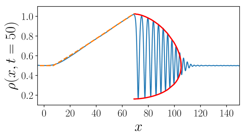
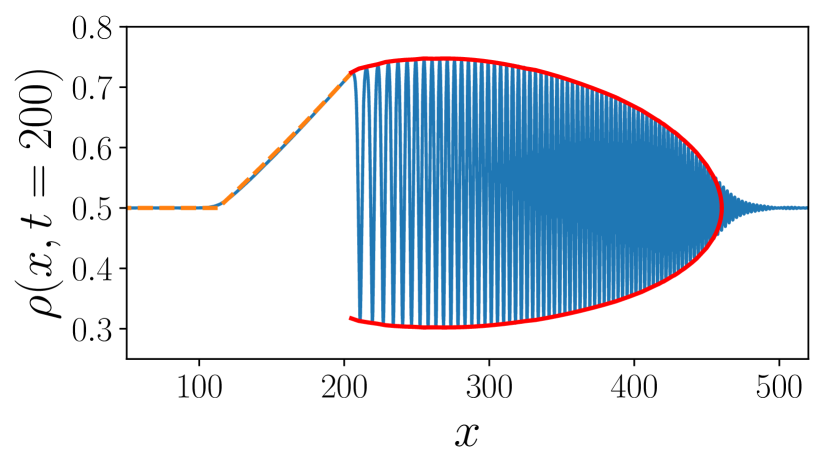
Figure 12: Comparison between theory and numerical simulations for the density profile $\rho(x,t)$ at $t=50$ (upper plot) and $t=200$ (lower plot). The initial profile is the same that was used in all the previous figures. The blue curves are the numerical results. The red solid lines are the envelopes of the density (52) where the $\lambda_{i}$’s are calculated by the procedure described in Sec. VI.4. The dashed orange lines correspond to the the dispersionless part of the profile, determined using the method exposed in Sec. III.

Figure 13: Wavelength of the nonlinear oscillations within the DSW for $t=200$. The theoretical red curve is calculated from Eq. (56). The blue points are extracted from simulations.

The corresponding density profiles are shown in Fig. 12 at different values of time for the initial distribution (3) (with $\rho_{0}=0.5$, $\rho_{1}=1.5$ and $x_{0}=20$). The agreement with the numerical simulation is excellent. The same level of accuracy is reached for the velocity profile $u(x,t)$.

In Fig. (13) we also compare the wavelength of the nonlinear oscillations within the DSW as determined by Whitham approach [Eq. (56)] with the results of numerical simulations, and the agreement is again very good.

VII Discussion and experimental considerations

The different situations we have identified are summarized in Fig. 14 which displays several typical density profiles in a “phase space” with coordinates $\rho_{1}/\rho_{0}$ and $t$. The curves $t_{\rm split}(\rho_{1}/\rho_{0})$ [as given by Eq. (49)] and $t_{\rm\scriptscriptstyle WB}(\rho_{1}/\rho_{0})$ [Eq. (72)] separate this plane in four regions, labeled as (a), (b), (c) and (d) in the figure. These two curves cross at a point represented by a white dot whose coordinates we determined numerically as being $\rho_{1}/\rho_{0}=0.60814$ and $c_{0}\,t/x_{0}=1.09623$. These coordinates are universal in the sense that they have the same value for any initial profile of inverted parabola type, such as given by Eq. (3), with $u(x,0)=0$. Other types of initial profile would yield different precise arrangements of these curves in phase space, but we expect the qualitative behavior illustrated by Fig. 14 to be generic, because the different regimes depicted in this figure correspond to physical intuition: a larger initial hump (larger $\rho_{1}/\rho_{0}$) experiences earlier wave breaking, and needs a longer time to be separated in two contra-propagating pulses. Also, the evolution of a small initial pulse can initially be described by perturbation theory and first splits in two humps which experience wave breaking in a later stage (as illustrated in Fig. 1): this is the reason why $t_{\rm split}<t_{\rm\scriptscriptstyle WB}$ for small $\rho_{1}/\rho_{0}$. In the opposite situation where $t_{\rm\scriptscriptstyle WB}<t<t_{\rm split}$, the wave breaking has already occurred while the profile has not yet split in two separated humps. This is the situation represented by the inset (b) and which has been considered in Refs. wkf-07 and Xu16 .

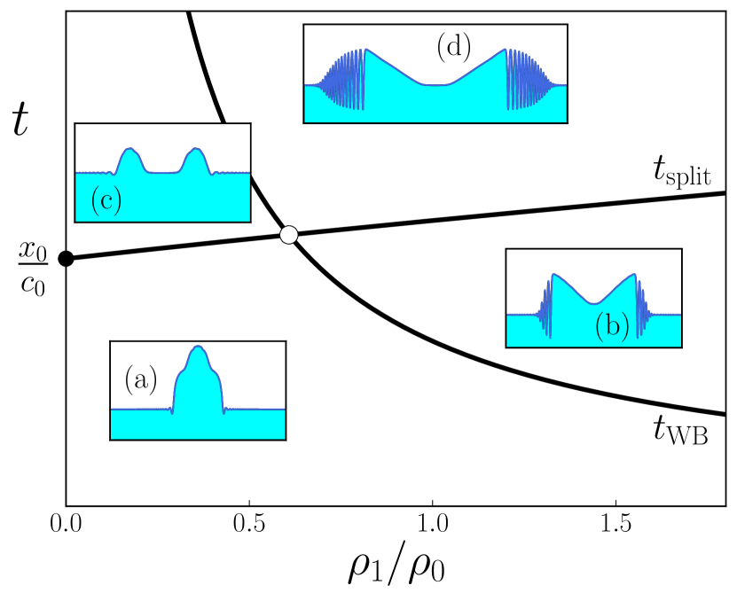
Figure 14: Behavior of the light intensity profile in the plane $(\rho_{1}/\rho_{0},t)$. The plane is separated in four regions by the curves $t=t{\rm\scriptscriptstyle WB}$ and $t=t_{\rm split}$. These curves cross at the point represented by a white dot (of coordinates $\rho_{1}/\rho_{0}=0.60814$ and $c_{0}\,t/x_{0}=1.09623$). Typical profiles are displayed in the insets (a), (b), (c) and (d) which represent $\rho(x,t)$ plotted as a function of $x$ for fixed $t$.

In Ref. Xu16 , Xu et al. studied the formation of a DSW in a nonlinear optic fiber remf0 varying the intensity of the background. In particular, they quantitatively evaluated the visibility of the oscillations near the solitonic edge of the DSW by measuring the contrast

$$C_{\rm ont}=\frac{\rho_{\rm max}-\rho_{\rm min}}{\rho_{\rm max}+\rho_{\rm min}}\;,$$ (106)

where $\rho_{\rm max}$ and $\rho_{\rm min}$ are defined in the inset of Fig. 15. In Ref. Xu16 , the contrast was studied for a fiber of fixed length, for an initial Gaussian bump — i.e., different from (3) — keeping the quantities analogous to $\rho_{1}$ and $x_{0}$ fixed and varying $\rho_{0}$. The experimental results agreed very well with numerical simulations taking into account absorption in the fiber. Here, we do not consider exactly the same initial profile and do not take damping into account, but we show that our approach gives a very reasonable analytic account of the behavior of $C_{\rm ont}$ considered as a function of $\rho_{0}/\rho_{1}$.

From Eq. (52) in the limit $m\to 1$ (which is the relevant regime near the solitonic edge of the DSW) one gets

$$\rho_{\rm max}=\tfrac{1}{4}(\lambda_{\scriptscriptstyle\rm S}+c_{0})^{2}\;,\;\;\mbox{and}\quad\rho_{\rm min}=\tfrac{1}{4}(\lambda_{\scriptscriptstyle\rm S}-3c_{0})^{2}\;,$$ (107)

yielding

$$C_{\rm ont}=\frac{4c_{0}(\lambda_{\scriptscriptstyle\rm S}-c_{0})}{(\lambda_{\scriptscriptstyle\rm S}-c_{0})^{2}+4c_{0}^{2}}\;.$$ (108)

The results presented in Fig. 15 demonstrate that, as expected, this expression (black solid line in the figure) agrees very well with the contrast determined from the numerical solution of Eq. (2) (green dots).

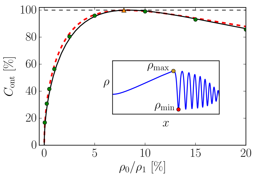
Figure 15: Contrast $C_{\rm ont}$ represented as a function of $\rho_{0}/\rho_{1}$. We follow here the procedure of Ref. Xu16 and use the same dimensionless parameters: the value of $\rho_{0}$ varies while $\rho_{1}=5.9$, $x_{0}=6.3$ and $t=9$ are fixed. The green dots correspond to the numerically determined value of the contrast, obtained from Eq. (106) where $\rho_{\rm min}$ and $\rho_{\rm max}$ are defined as illustrated in the inset. The black solid line corresponds to expression (108), where $\lambda_{\scriptscriptstyle\rm S}$ is obtained from (77). The red dashed line is the approximate result obtained from the same Eq. (108), but evaluating $\lambda_{\scriptscriptstyle\rm S}$ from Eqs. (81), (110) and (112). The triangle marks the point of contrast unity.

At this point, the computation of $C_{\rm ont}$ through (108) relies on the determination of $\lambda_{\scriptscriptstyle\rm S}$ by means of (77), a task which requires a good grasp of the Riemann approach. However, one can get an accurate, though approximate, analytic determination of $C_{\rm ont}$ in a simpler way: by using the large time expression (81) for $\lambda_{\scriptscriptstyle\rm S}$, together with the approximation

$$\begin{split}\cal A\simeq&-\Bigg{(}\int_{c_{m}}^{c_{0}}\sqrt{r-c_{0}}\,\frac{dw^{\scriptscriptstyle\rm B}(r)}{dr}dr\\ &+\int_{c_{0}}^{c_{m}}\sqrt{r-c_{0}}\,\frac{dw^{\scriptscriptstyle\rm A}(r)}{dr}dr\Bigg{)}\\ =&\;2\int_{0}^{x_{0}}\sqrt{\lambda^{+}(x,0)-c_{0}}\;dx.\end{split}$$ (109)

In the above, we approximated in expression (80) $W_{+}^{(3/2)}(-c_{0},r)$ by $w^{\scriptscriptstyle\rm A/B}(r)$, used the symmetry of these functions and made the change of variable $x=w^{\scriptscriptstyle\rm A}(r)\Leftrightarrow r=\lambda^{+}(x,0)$, in which $\lambda^{+}(x,0)=\sqrt{\rho}(x,0)$ where $\rho(x,0)$ is the initial density profile (3). A new change of variable yields

$${\cal A}\simeq 2x_{0}\sqrt{c_{0}}\,F(\rho_{0}/\rho_{1})\;,$$ (110)

where

$$F(\alpha)=\int_{0}^{\pi/2}\cos\theta\left(\sqrt{1+\frac{\cos^{2}\theta}{\alpha}}-1\right)^{1/2}\!\!d\theta.$$ (111)

A simple analytic expression of $F(\alpha)$ cannot be obtained, but we checked that one can devise an accurate approximation by expanding the term in parenthesis in the above integrand around $\theta=0$ up to second order in $\theta$. This yields

$$\begin{split}F(\alpha)\simeq&\;\frac{(\sqrt{\alpha+1}-\sqrt{\alpha})^{1/2}}{\alpha^{1/4}}\\ &-\frac{\tfrac{1}{4}(\pi^{2}/4-2)}{\alpha^{1/4}\sqrt{1+\alpha}(\sqrt{\alpha+1}-\sqrt{\alpha})^{1/2}}\;.\end{split}$$ (112)

In the domain $10^{-3}\leq\alpha\leq 50$, $F(\alpha)$ varies over two orders of magnitude (from 4.8 to $7.8\times 10^{-2}$), and the approximation (112) gives an absolute error ranging from $5.8\times 10^{-2}$ to $1.8\times 10^{-3}$, and a relative one ranging from 1.1 % to 2.4 %.

Combining Eqs. (108), (81), (110) and (112) yields an analytic expression for the contrast $C_{\rm ont}$. This expression is represented as a dashed red line in Fig. 15. As one can see, it compares quite well with the value of $C_{\rm ont}$ extracted from the numerical simulations remf . The better agreement with the numerical result is reached for small $\rho_{0}/\rho_{1}$; this was expected: in this regime the wave breaking occurs rapidly, and one easily fulfils the condition $t\gg t_{\rm\scriptscriptstyle WB}$ where the approximation (81) holds. We note here that the behavior of the contrast illustrated in Fig. 15 is very similar to the one obtained in Ref. Xu16 . In both cases there is a special value of $\rho_{0}/\rho_{1}$ for which the contrast is unity, meaning that the quantity $\rho_{\rm min}$ cancels. From (107) and (81) this is obtained for $2c_{0}\simeq({\cal A}/t)^{2/3}$, i.e. - using (110) – for

$$\frac{c_{0}\,t}{x_{0}}=\frac{1}{\sqrt{2}}\,F(\rho_{0}/\rho_{1})\;.$$ (113)

A numerical solution of this equation gives, for the parameters of Fig. 15, a contrast unity when $\rho_{0}/\rho_{1}=7.9$ %, while the exact Eq. (108) predicts a maximum contrast when $\rho_{0}/\rho_{1}=8.3$ % instead (the exact result at $\rho_{0}/\rho_{1}=7.9$ % is $C_{\rm ont}=0.999$). These two values are marked with a single triangle in Fig. 15 because they cannot be distinguished on the scale of the figure. This shows that the solution of Eq. (113) gives a simple way for determining the best configuration for visualizing the fringes of the DSW; this should be useful for future experimental studies.

Note that formula (108) demonstrates that the contrast depends only on $\lambda_{\scriptscriptstyle\rm S}/c_{0}$, and using the approximate relations (81) and (113) leads to the conclusion that $C_{\rm ont}$ can be considered as a function of the single variable

$$X=\frac{x_{0}}{t\sqrt{\rho_{1}}}\sqrt{\frac{\rho_{1}}{\rho_{0}}}F(\rho_{0}/\rho_{1})\;.$$ (114)

Hence, for a configuration different from the one considered in Fig. 15 but for which the combination of parameters $t\,\sqrt{\rho_{1}}/x_{0}$ takes the same value (namely 3.47), the curve $C_{\rm cont}(\rho_{0}/\rho_{1})$ should superimpose with the one displayed in Fig. 15. We checked that this is indeed the case by taking $\rho_{1}=2$, $x_{0}=20$ and $t=49$, but did not plot the corresponding contrast in Fig. 15 for legibility.

Fig. 15 and the discussion of this section illustrate the versatility of our approach which, not only gives an excellent account of the numerical simulations at the prize of an elaborate mathematical treatment, but also provides simple limiting expressions — such as Eq. (81) — which make it possible to obtain an analytic and quantitative description of experimentally relevant parameters such as the contrast of the fringes of the DSW.

VIII Conclusion

In this work we presented a detailed theoretical treatment of the spreading of a light pulse propagating in a nonlinear medium. A hydrodynamic approach to both the initial nondispersive spreading and the subsequent formation of an optical dispersive shock compares extremely well with the results of numerical simulations. Although in reality the transition between these two regimes is gradual, it is sharp within the Whitham approximation. An exact expression has been obtained for the theoretical wave breaking time which separates these two regimes [Eq. (72)], which may be used for evaluating the experimental parameters necessary for observing a DSW in a realistic setting (see Fig. 14). Besides, our theoretical treatment provides valuable insight into simple features of the shocks which are relevant to future experimental studies, such as the coordinates of its trailing edge $x_{\scriptscriptstyle\rm S}$, the large-time nondispersive intensity profile which follows it (Sec. V), and the best regime for visualizing the fringes of the DSW (Sec. VII). We note also that our treatment reveals the existence of an asymptotically conserved quantity which had remained unnoticed until now, see Eq. (84).

A possible extension of the present work would be to consider an initial configuration for which, at variance with the situation we study here, the largest intensity gradient is not reached exactly at the extremity of the initial hump. In this case, wave breaking occurs within a simple wave (not at its boundary), and the DSW has to be described by four position and time dependent Riemann invariants ek-95 . In vicinity of the wave breaking moment, one of the Riemann invariants can be considered as constant, and a generic dispersionless solution can be represented by a cubic parabola; for this simpler case the detailed theory was developed in Ref. kku-02 . In Refs. ekv-01 ; Gra07 the general situation was considered for the Korteweg-de Vries equation.

We conclude by stressing that the present treatment focuses on quasi-one dimensional spreading; future developments should consider non exactly integrable systems, for instance light propagation in a photorefractive medium, in a bi-dimensional situation with cylindrical symmetry. Work in these directions is in progress.

- (1) V. I. Talanov, Radiophys. 9, 138 (1965).
- (2) S. A. Akhmanov, A. P. Sukhorukov and R. V. Khokhlov, Zh. Eksp. Teor. Fiz. 50, 1537 (1966) [Sov. Phys. JETP 23, 1025 (1966)].
- (3) S. A. Akhmanov, A. P. Sukhorukov and R. V. Khokhlov, Usp. Fiz. Nauk 93, 19 (1967) [Sov. Phys. Usp. 10, 609 (1968)] doi:10.1070/PU1968v010n05ABEH005849
- (4) S. A. Akhmanov, D. P. Krindach, A. P. Sukhorukov, and R. V. Khokhlov Pis’ma Zh. Eksp. Teor. Fiz. 6, 509 (1967) [JETP Lett. 6, 38 (1967)].
- (5) R.G. Harrison, L. Dambly, Dejin Yu, Weiping Lu, Opt. Commun. 139, 69 (1997) doi:10.1016/S0030-4018(96)00790-0
- (6) P. Emplit, J. P. Hamaide, F. Reynaud, C. Froehly, and A. Barthelemy, Opt. Commun. 62, 374 (1987) doi:10.1016/0030-4018(87)90003-4
- (7) D. Krökel, N. J. Halas, G. Giuliani, and D. Grischkowsky Phys. Rev. Lett. 60, 29 (1988) doi:10.1103/PhysRevLett.60.29
- (8) A. M. Weiner, J. P. Heritage, R. J. Hawkins, R. N. Thurston, E. M. Kirschner, D. E. Leaird, and W. J. Tomlinson, Phys. Rev. Lett. 61, 2445 (1988) doi:10.1103/PhysRevLett.61.2445
- (9) F. T. Arecchi, G. Giacomelli, P. L. Ramazza, and S. Residori Phys. Rev. Lett. 67, 3749 (1991) doi:10.1103/PhysRevLett.67.3749
- (10) M. Vaupel, K. Staliunas, and C. O. Weiss Phys. Rev. A 54, 880 (1996) doi:10.1103/PhysRevA.54.880
- (11) D. Vocke, K. Wilson, F. Marino, I. Carusotto, E. M. Wright, T. Roger, B. P. Anderson, P. Öhberg, D. Faccio, Phys. Rev. A 94, 013849 (2016) doi:10.1103/PhysRevA.94.013849.
- (12) J. E. Rothenberg, and D. Grischkowsky, Phys. Rev. Lett. 62, 531 (1989) doi:10.1103/PhysRevLett.62.531
- (13) N. Ghofraniha, C. Conti, G. Ruocco, and S. Trillo, Phys. Rev. Lett. 99, 043903 (2007) doi:10.1103/PhysRevLett.99.043903
- (14) G. Couton, H. Maillotte, and M. Chauvet, J. Opt. B: Quantum Semiclassical Opt. 6, S223 (2004), doi:10.1088/1464-4266/6/5/009.
- (15) W. Wan, S. Jia, and J. W. Fleischer, Nature Phys. 3, 46 (2007), doi:10.1038/nphys486.
- (16) C. Barsi, W. Wan, C. Sun, and J. W. Fleischer, Opt. Lett. 32, 2930 (2007), doi:10.1364/OL.32.002930
- (17) J. Fatome, C. Finot, G. Millot, A. Armaroli, and S. Trillo, Phys. Rev. X 4, 021022 (2014) doi:10.1103/PhysRevX.4.021022.
- (18) G. Xu, A. Mussot, A. Kudlinski, S. Trillo, F. Copie, and M. Conforti, Opt. Lett. 41, 2656 (2016), doi:10.1364/OL.41.002656
- (19) G. Xu, M. Conforti, A. Kudlinski, A. Mussot, S. Trillo, Phys. Rev. Lett. 118, 254101 (2017) doi:10.1103/PhysRevLett.118.254101
- (20) M. Karpov, T. Congy, Y. Sivan, V. Fleurov, N. Pavloff and S. Bar-Ad, Optica 2, 1053 (2015) doi:10.1364/OPTICA.2.001053
- (21) M. Elazar, V. Fleurov, S. Bar-Ad, Phys. Rev. A 86, 063821 (2012) doi:10.1103/PhysRevA.86.063821
- (22) D. Vocke, C. Maitland, A. Prain, F. Biancalana, F. Marino, E. M. Wright, D. Faccio, Optica 5, 1099 (2018) doi:10.1364/OPTICA.5.001099
- (23) J. Drori, Y. Rosenberg, D. Bermudez, Y. Silberberg, and U. Leonhardt, Phys. Rev. Lett. 122, 010404 (2019), doi:10.1103/PhysRevLett.122.010404
- (24) D. Vocke, T. Roger, F. Marino, E. M. Wright, I. Carusotto, M. Clerici, and D. Faccio, Optica 2, 484 (2015) doi:10.1364/OPTICA.2.000484
- (25) Q. Fontaine, T. Bienaimé, S. Pigeon, E. Giacobino, A. Bramati, and Q. Glorieux, Phys. Rev. Lett. 121, 183604 (2018) doi:10.1103/PhysRevLett.121.183604.
- (26) C. Michel, O. Boughdad, M. Albert, P.-É. Larré, and M. Bellec, Nat. Commun. 9, 2108 (2018) doi:10.1038/s41467-018-04534-9
- (27) A. M. Kamchatnov, A. Gammal, and R. A. Kraenkel, Phys. Rev. A 69, 063605 (2004) doi:10.1103/PhysRevA.69.063605.
- (28) G. A. El, A. Gammal, E. G. Khamis, R. A. Kraenkel, and A. M. Kamchatnov, Phys. Rev. A 76, 053813 (2007) doi:10.1103/PhysRevA.76.053813
- (29) M. Conforti and S. Trillo in Rogue and Shock Waves in Nonlinear Dispersive Media, M. Onorato, S. Residori and F. Baronio eds., Lecture Notes in Physics Volume 926, (Springer International Publishing, Switzerland 2016).
- (30) G. B. Whitham, Linear and Nonlinear Waves (Wiley Interscience, New York, 1974).
- (31) M. Isoard, A. M. Kamchatnov, and N. Pavloff, Phys. Rev. E 99, 012210 (2019) doi:10.1103/PhysRevE.99.012210
- (32) G. S. S. Ludford, Proc. Camb. Phil. Soc. 48, 499 (1952) doi:10.1017/S0305004100027900
- (33) M. G. Forest, C.-J. Rosenberg, and O. C. Wright III, Nonlinearity 22, 2287 (2009), doi:10.1088/0951-7715/22/9/012
- (34) A. V. Gurevich and L. P. Pitaevskii, Zh. Eksp. Teor. Fiz. 65, 590 (1973) [Sov. Phys. JETP 38, 291 (1974)].
- (35) G. A. El and M. A. Hoefer, Physica D 333, 11 (2016), doi:10.1016/j.physd.2016.04.006
- (36) A. V. Gurevich, A. L. Krylov, and N. G. Mazur, Zh. Eksp. Teor. Fiz. 95, 1674 (1989) [Sov. Phys. JETP 68, 966 (1989)].
- (37) A. V. Gurevich, A. L. Krylov and G. A. El, Pis’ma Zh. Eksp. Teor. Fiz. 54, 104 (1991) [JETP Lett. 54, 102 (1991)].
- (38) A. V. Gurevich, A. L. Krylov and G. A. El, Zh. Eksp. Teor. Fiz. 101, 1797 (1992) [Sov. Phys. JETP 74, 957 (1992)].
- (39) A. L. Krylov, V. V. Khodorovskii and G. A. El, Pis’ma Zh. Eksp. Teor. Fiz. 56, 325 (1992) [JETP Lett. 56, 323 (1992)].
- (40) G. A. El and V. V. Khodorovsky, Phys. Lett. A 182, 49 (1993), doi:10.1016/0375-9601(93)90051-Z.
- (41) G. A. El, A. M. Kamchatnov, V. V. Khodorovskii, E. S. Annibale, and A. Gammal, Phys. Rev. E 80, 046317 (2009), doi:10.1103/PhysRevE.80.046317.
- (42) L. D. Landau and E. M. Lifshitz, Electrodynamics of Continuous Media, Course of Theoretical Physics vol. 8 (Elsevier Butterworth-Heinemann, Oxford, 2006).
- (43) S. P. Tsarev, Math. USSR Izv. 37, 397 (1991), doi:10.1070/IM1991v037n02ABEH002069.
- (44) A. Sommerfeld, Partial Differential Equations in Physics, (Lectures on Theoretical Physics volume VI) (Academic Press, New York, 1964).
- (45) M. Abramowitz and I. A. Stegun, Handbook of mathematical functions”, (Dover Publications, New York, 1970).
- (46) A. M. Kamchatnov, Nonlinear Periodic Waves and Their Modulations—An Introductory Course, (World Scientific, Singapore, 2000).
- (47) L. D. Landau and E. M. Lifshitz, Fluid Mechanics, (Pergamon, Oxford, 1987).
- (48) It should not be a surprise that, for determining the wave breaking time, it is legitimate to replace by in Eq. (45). Indeed, the wave breaking phenomenon occurs when several characteristics issued from the right region of the edge of the bump cross (in region III for the case considered). For all these characteristics, one intuitively expects that one can neglect the weak dependence of on ; this is indeed the case: one can rigorously show that and coincide in the limit , which is the relevant one for evaluating (45).
- (49) M. G. Forest and J. E. Lee, Geometry and modulation theory for periodic nonlinear Schrödinger equation, in Oscillation Theory, Computation, and Methods of Compensated Compactness, Eds. C. Dafermos et al., IMA Volumes on Mathematics and its Applications 2, p. 35 (Springer, N.Y., 1986). doi:10.1007/978-1-4613-8689-6_3.
- (50) M. V. Pavlov, Teor. Mat. Fiz. 71, 351 (1987) [Theoret. Math. Phys. 71, 584 (1987)] doi:10.1007/BF01017090.
- (51) R. Z. Sagdeev, Cooperative Phenomena and Shock Waves in Collisionless Plasmas, in Reviews of Plasma Physics, Ed. M. A. Leontovich, Vol. 4, p. 23, (Consultants Bureau, New York, 1966).
- (52) G. A. El and A. L. Krylov, Phys. Lett. 203, 77 (1995) doi:10.1016/0375-9601(95)00379-H.
- (53) O. C. Wright, Commun. Pure Appl. Math. 46, 423 (1993) doi:10.1002/cpa.3160460306
- (54) F. R. Tian, Commun. Pure Appl. Math. 46, 1093 (1993) doi:10.1002/cpa.3160460802.
- (55) L. P. Eisenhart, Ann. Math. 120, 262 (1918).
- (56) G. Arfken and H. J. Weber, Mathematical Methods for Physicists (Academic Press, Orlando, 2005).
- (57) G. A. El, Chaos 15, 037103 (2005), doi:10.1063/1.1947120; ibid. 16, 029901 (2006), doi:10.1063/1.2186766.
- (58) A. M. Kamchatnov, Phys. Rev. E 99, 012203 (2019) doi:10.1103/PhysRevE.99.012203
- (59) In this case the role of variable in Eq. (2) is played by time, but the phenomenology is very similar to the one we describe in the present work, see, e.g., Y. S. Kivshar and G. P. Agrawal, Optical Solitons (Academic Press, San Diego, 2003).
- (60) Computing the contrast using expression (111) instead of the approximation (112) yields a result which is barely distinguishable from the dashed line in Fig. 15.
- (61) A. M. Kamchatnov, R. A. Kraenkel and B. A. Umarov, Phys. Rev. E 66, 036609 (2002) doi:10.1103/PhysRevE.66.036609.
- (62) G. A. El, A. L. Krylov, and S. Venakides, Commun. Pure Appl. Math. 54, 1243 (2001) doi:10.1002/cpa.10002.
- (63) T. Grava and C. Klein, Comm. Pure Appl. Math. 60, 1623 (2007) doi:10.1002/cpa.20183.