A stochastic individual based model for the growth of a stand of Japanese knotweed including mowing as a management technique.

Abstract

Invasive alien species are a growing threat for environment and health. They also have a major economic impact, as they can damage many infrastructures. The Japanese knotweed (Fallopia japonica), present in North America, Northern and Central Europe as well as in Australia and New Zealand, is listed by the World Conservation Union as one of the world’s worst invasive species. So far, most models have dealt with how the invasion spreads without management. This paper aims at providing a model able to study and predict the dynamics of a stand of Japanese knotweed taking into account mowing as a management technique. The model we propose is stochastic and individual-based, which allows us taking into account the behaviour of individuals depending on their size and location, as well as individual stochasticity. We set plant dynamics parameters thanks to a calibration with field data, and study the influence of the initial population size, the mean number of mowing events a year and the management project duration on mean area and mean number of crowns of stands. In particular, our results provide the sets of parameters for which it is possible to obtain the stand eradication, and the minimal duration of the management project necessary to achieve this latter.

1 Introduction

Invasive alien species are a growing problem for environment and health. They may cause a loss of biodiversity (Murphy and Romanuk, 2014), changes in ecosystem functioning (Strayer, 2012) or affect human well-being (Shackleton et al., 2019). They also have a major economic impact (Kettunen et al., 2008; Pimentel et al., 2005). The necessity to act against invasive species relies on their global and local impacts and also on international policy engagements. For example, since 1992, the Convention on Biological Diversity (article 8) compels the parties to "prevent the introduction of, control or eradicate those alien species which threaten ecosystems, habitats or species". Invasive species management raises several issues and strategies depend on the species, the step reached on the invasion process and the scale of action (Simberloff et al., 2013).

Together with field experiments, mathematical models can provide a better understanding of the critical determinants of the growth and spread of these species and thus help to identify efficient management strategies. Many studies focus on optimal management of invasive species (Baker and Bode, 2016; Harris et al., 2009; Travis et al., 2011). Control strategies aim at bringing the density of the invasive species below a threshold. For seed dispersal species, a frequent question in the literature of invasive species through mathematical modelling is to assess the benefit of a spatial prioritization: is it more profitable to remove the individuals at the heart of the infection, or those on the periphery (Harris et al., 2009) ? The answer depends essentially on the spatial spread of the plant (and therefore on the species considered). Another issue in the literature of invasive species management is the temporal distribution of the effort: is it better to act significantly at the beginning of the management project and then to control the invasion with a lower effort (as in Meier et al. (2014)), or to increase the effort over time (as in Baker and Bode (2016))? A common assumption when dealing with control strategies is that the invasive species has already been present for a long time (Baker and Bode, 2016). We know however that early detection and rapid response to the invasion may have a greater efficiency (Pyšek and Richardson, 2010).

Among the worst invasive species threatening biodiversity, Asian knotweeds raise particular management issues. This complex of three species (the Japanese knotweed, Fallopia japonica [Houtt.] Ronse Decraene, the giant knotweed, Fallopia sachalinensis [Schmidt Petrop.] Ronse Decraene and the hybrid between the two previous the Bohemian knotweed (Fallopia $\times$ bohemica Chrtek & Chrtkova) have invaded Europe and North America. Native to Eastern Asia, knotweeds have been introduced for ornamental purpose at the end of the 19th century (Bailey and Wisskirchen, 2006; Barney et al., 2006; Beerling et al., 1994). They are also present in Australia, New Zealand and Chile (Alberternst and Böhmer, 2006; Saldaña et al., 2009).

Asian knotweeds quickly invade the environment in which they grow (Gowton et al., 2016) and have large impacts (Lavoie, 2017). They displace other plant species through light competition and allelopathy (Dommanget et al., 2014; Siemens and Blossey, 2007), affect native fauna diversity (Abgrall et al., 2018; Gerber et al., 2008; Maerz et al., 2005; Serniak et al., 2017) and modify ecosystem functioning (Dassonville et al., 2011; Tharayil et al., 2013). In addition, the control costs are very high and were estimated at 250 million dollars a year in Great Britain (Colleran and Goodall, 2014) and more than 2 billion euros a year in Europe (Kettunen et al., 2009).

Asian knotweeds grow in a wide variety of soils: sandy, swampy, rocky. They mainly invade human modified habitats such as roadsides, waste dumps, but also river banks. They are perennial geophytes: their rhizomes allow them to spend the winter season buried in the ground (De Waal, 2001). Their rhizomes also play a major role in their propagation, thanks to their strong regeneration capacities (Bailey et al., 2009; Brock et al., 1992). Once arrived in a new area, the rhizome expands centrifugally and a new stand can sustainably establish in a few weeks (Gowton et al., 2016; Smith et al., 2007).

Once established and due to their extensive rhizome network, Asian knotweeds are extremely hard to remove. Rhizomes represent two third of their biomass (Barney et al., 2006) and can expand several meters away from the visible invasion front (Barney et al., 2006). The resources they store can be efficiently remobilized after mowing events (Rouifed et al., 2011). Some authors estimate that six cuttings are needed to significantly reduce belowground biomass (Gerber et al., 2010). Understanding the underground development of Asian knotweeds is crucial to gain insight in their local propagation and performance. Moreover it could help to better design efficient management strategies.

As underground organs are almost inaccessible to observers, direct observations are scarce and models could help to approach their dynamics and better understand how management actions can affect their development. To our knowledge, there are very few models in the literature that describe the growth of a Japanese knotweed stand, and among them, rare are those that include a management technique.

In Smith et al. (2007), the authors build a 3D correlated random walk model of the development of the subterranean rhizome network for a single stand of Japanese knotweed. Their model is based on knowledge of the morphology and physiology of the plant. They study the model through simulations and they observe a quadratic expansion of the area invaded.

Dauer and Jongejans (2013) propose an "Integral Projection Model", inspired from matrix population models, for the plant dynamics at the level of a stand. The variable of interest is a continuous variable which stands for the height or the total biomass of the plant, and the authors use a simplified plant life cycle to model transition between states, like the transition from new shoots to crown (a crown is the location of a terminal bud from which stems emerge). They study the parameters that have the largest effect on the growth rate of the population.

Gourley et al. (2016) develop a mathematical model for biocontrol of Fallopia japonica using one of its co-evolved natural enemies, the Japanese sap-sucking psyllid Aphalara itadori. It is a deterministic model that describes the evolution of the number of insects (larvae and adults), the total weight of the knotweed stems and the rhizome biomass. A key parameter of their model is the duration that a larva takes to consume and digest the rhizome biomass of the plant.

A commonly used management technique for Asian knotweed stands is mowing. Managers can vary its intensity and frequency, which motivates a study of the effects of these two parameters on the dynamics of the stand. This paper aims at understanding the influence of mowing on the growth of a Asian knotweed stand. More precisely, we study the influence of the initial population size, the mean number of mowing events a year and the management project duration on mean area and mean number of crowns of the stands. To our knowledge, existing models are not well designed to study such questions. Here we present a stochastic individual based model for the growth of a stand of Japanese knotweed including mowing as a management technique. The stochastic formalism enables us to study the early stage of invasion, without assuming the species has been present for a long time. The description of phenomena at the level of individuals enables us to take into account the variability between crowns, for example due to different ages. The study will focus on the influence of management parameters on model outputs which are area and number of crowns of the stand.

The paper is organized as follows. Section 2 is devoted to the description of the ecological mechanisms taken into account in the model (apical dominance, intraspecific competition, etc.), the presentation of the mathematical model, as well as the methods we used for our study. Results are given in Section 3. In particular, we performed a calibration of the plant dynamics with field data from stands observed in the French Alps. We also studied, using numerical simulations with OpenMOLE software (Reuillon et al., 2013), the influence of management parameters on the population growth. Finally, we summarize our results and discuss their implications and shortcomings in Section 4.

2 Materials and methods

In this section we provide a description of the dynamical model for the growth of a stand of Japanese knotweed including mowing as a management technique. We also describe the methods used to its study through numerical simulations.

In the sequel, the term individual will refer to crowns, we recall that a crown is the location of a terminal bud from which stems emerge. Individuals are characterized by their position $x$ in the plane and their underground biomass $a$ (i.e. the biomass rhizome connected to the crown).

The following notations will be needed to describe our model:

• $\chi=\mathbb{R}^{2}\times\mathbb{R}_{+}$, is the state space of positions and biomasses. In the model, a crown is represented by a Dirac mass $\delta_{(x,a)}$, with $(x,a)\in\chi$, where $x$ stands for the position of the crown and $a$ is the biomass associated with the crown.

• The set of crowns present at time $t$ is described by the measure $Z_{t}\in\mathcal{M}(\chi)$, where $\mathcal{M}(\chi)$ is the set of finite point measures on $\chi$ whose masses of points are 0 or 1.

  $$\mathcal{M}(\chi)=\left\{\sum_{i=1}^{n}\delta_{(x_{i},a_{i})}~{},~{}n\geq 0,~{}(x_{1},a_{1}),\ldots,(x_{n},a_{n})\in\chi\right\}.$$

• $\mathcal{M}_{F}(\chi)$ [resp. $\mathcal{P}(\chi)$] is the set of finite measures (resp. probability measures) on $\chi$, such that $\mathcal{M}(\chi)\subset\mathcal{M}_{F}(\chi)$.

Using $\mathcal{M}_{F}(\chi)$ allows us not setting a priori the number of individuals in the model, since it contains all the possible population sizes, $n\geq 0$.

2.1 Description of the phenomena included in the model

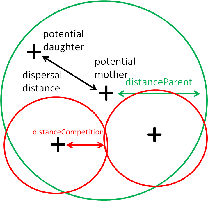
Birth: an individual with trait $(x,a)\in\chi$ (i.e. its position is $x$ and it has an underground biomass $a$) will give birth at the rate $b(x,Z)$, where $Z\in\mathcal{M}(\chi)$ describes the state of the system (i.e. the positions and biomasses of all individuals). It is assumed here that this birth rate does not depend on $a$. A crown can give birth to several crowns and the rates at which an individual gives birth takes into account the proximity with its neighbouring individuals. Based on Smith et al. (2007), we consider that a crown will give birth to at most two daughter crowns. We introduce the real parameter $distanceParent$, so that the birth rate of a crown depends on the number of crowns that are at a distance smaller than $distanceParent$ from it. So, if a crown has already given birth to its two daughters (in fact if there are already three individuals which are at a distance smaller than $distanceParent$ from it since we count its parent), it will have a zero birth rate (it does not give birth anymore). We will see in the next paragraph that a daughter crown can in principle be at a distance greater than $distanceParent$ from its parent. This phenomenon may be balanced by the fact that crowns from another parent can be at a distance less than $distanceParent$. This modelling allows us to account for the effects of apical dominance: if a crown dies, the apical dominance it exerts on the neighbouring lateral buds ceases, and these last ones may develop to form aerial shoots, and thus form a new crown.

Bashtanova et al. (2009), Adachi et al. (1996) and Dauer and Jongejans (2013) mention this phenomenon of apical dominance in a general way, but they do not specify a typical distance. That is why we will use a calibration method to set its value (in fact we use this method for all parameters, cf. Section 2.4).

The rate at which an individual with position $x$ gives birth can thus be expressed as follows:

$$b(x,Z)=\bar{b}_{\{\sum_{y\in V(Z)}1_{\{|x-y|\leq distanceParent\}}~{}\leq 3\}},$$ (1)

where

$$V(Z):=\{x\in\mathbb{R}^{2},Z(\{x\}\times\mathbb{R}_{+})>0\}$$

is the set of the positions of the crowns present in the population $Z$.

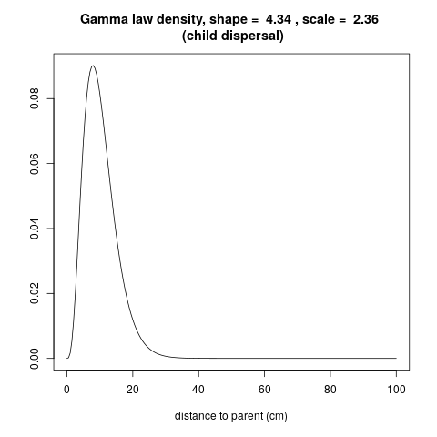
Dispersal of the created individual: an individual with trait $(x,a)$ which gives birth generates an individual at position $x^{\prime}$. Here we choose a Gamma law density denoted by $D$ for the birth distance law. The parameters ($shape$, $scale$) of the law will be subject to calibration. We assume a uniform distribution on $x^{\prime}-x$ direction angle to the X-axis.

Moreover, we will model the phenomenon of intra-specific competition by considering that an individual is really born if it does not fall too close to an already existing crown (otherwise we consider that it is not born). So we introduce the set $C$ depending on the population state $Z$ and position of the potential parent $x$:

$$C_{x,Z}=\{z\in\mathbb{R}^{2},~{}\forall y\in V(Z)\setminus\{x\},~{}~{}|y-z|>distanceCompetition\}.$$ (2)

The individual created must therefore be at a distance larger than $distanceCompetition$ from its neighbours not to fall in the zone of intraspecific competition. This principle of excluded zones (for the birth of an individual) is also used in Smith et al. (2007): the zones surrounding the crowns are subject to competition for light and the appearance of new crowns is not allowed.

The diagram in Figure 1 shows distances playing a role during a birth event.

Figure 1: Diagram representing a birth event. A cross stands for a crown position. We also indicate the different distances used in the model.

Evolution of the biomass: in Seiger et al. (1997), the authors present the effects of mowing on rhizome growth. They find that rhizome biomass increases significantly throughout the growing season, unlike above-ground biomass, which no longer grows significantly at the end of the summer. If the aerial shoots are not cut, the growth of the underground biomass $a$ is assumed to evolve according to a Von Bertalanffy’s law (Paine et al., 2012), presented below (Equation (4)). The effects on rhizome development of mowing aerial shoots are not well known. We assume that mowing results in a decrease of underground biomass. This assumption stems from the fact that rhizome resources are used for aerial shoot regeneration (see Gerber et al. (2010)). In Rouifed et al. (2011), the authors also note that mowing impacts the amount of underground biomass at the end of the season, and that mowing induces a decreasing rhizome density with depth (whereas without mowing it is constant). However, we do not take this phenomenon into account, since the model is planar.

Mowing events occur at a rate $1/\tau$ (there is thus a mean of $\tau$ mowing events a year), and a proportion $proportionMowing$ (constant) of individuals is mown.

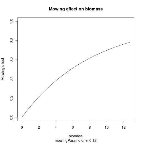
After a mowing event, it is assumed that the underground biomass $a$ of an individual is immediately impacted and becomes $a.F(a)$, where $F$ takes values in $[0,1]$ and describes the mowing effect as a function of the individual biomass. In order to take into account the fragility of young crowns, it is assumed that the function $F$ describing the impact of mowing on biomass is higher for low biomasses (we therefore take $F$ increasing, which implies that for two biomasses $a_{1}<a_{2}$, we will have $a_{1}*F(a_{1})<a_{2}*F(a_{2})$). We suppose that $F$ has the form:

$$\forall a\in\mathbb{R}_{+},~{}F(a)=1-exp(-mowingParameter*a),$$ (3)

where $mowingParameter$ is a parameter that acts on the decay rate of the exponential function.

We now have to specify how we choose the crowns to be mown. In this paper, we consider two possibilities. The first one is to choose the mowed crowns uniformly at random (random management technique). The proportion can thus represent different qualities of mowing if the aim is to mow the whole stand, with respect to different tools used (by hand, brush cutter). We consider this technique when we write the mathematical formalism of the model in Section 2.2. The second one is mowing one side of the stand: it consists in determining an abscissa at the right of which every crown is mowed, and at the left of which no crown is mowed (side management technique). It reflects for example the case of a stand located on two plots, owned by different persons, one who manages the stand whereas the other does not. This situation occurs frequently along roadsides. We use this management technique in the model for the calibration due to the characteristics of our data set.

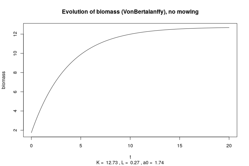
For the biomass growth of a crown when there is no mowing, we use Von Bertalanffy’s Equation (4). First described in von Bertalanffy (1934), this equation has then been very often used especially in forestry (Zeide, 1993). Here, this equation describes the evolution of the biomass as a function of time. It is based on simple physiological arguments: the growth rate of the organism decreases with biomass.

$$\frac{da(t)}{dt}=L(K-a(t))=:v(a(t)),$$ (4)

where $L$ is the growth rate at low biomass and $K$ is the maximal asymptotic biomass.

We can solve exactly Equation (4). If we suppose that the biomass at time $t_{0}$ is equal to $a_{0}$, then for all $t\geq t_{0}$, we get:

$$a(t)=a_{0}e^{-L(t-t_{0})}+K(1-e^{-L(t-t_{0})}).$$ (5)

Moreover, we assume that all crowns are born with the same biomass $a_{0}\in\mathbb{R}^{+}$.

Mortality: we assume that the mortality rate is independent of the individual position. An individual alive at time $t$ and with biomass $a(t)$ dies at a rate $m(a(t))$. We assume that the mortality $m$ is a decreasing function of the biomass: an individual with a low biomass, either because it has just been created or because it has been mown, has a higher mortality rate. So if $T_{0}$ is the date at which an individual born at time $0$ dies, and whose biomass up to time $t$ is given by the function $a$ (we suppose it is not mown), we get:

$$\mathbb{P}(T_{0}\geq t)=e^{-\int_{0}^{t}m(a(s))~{}ds}.$$ (6)

In Smith et al. (2007), the authors set the probability that a segment of rhizome dies over a four month period (a time step in their model) to 0.0083. When there is no mowing, mortality events for crowns rarely occur in nature, that is why the value proposed in Smith et al. (2007) is low. Having a good estimate for this value requires sufficiently large numbers of observations, thus calibration is very useful to estimate a value for such a parameter. We suppose that $m$, the function that describes the mortality rate of a crown according to its biomass, has the form:

$$m(a)=deathParameterScaling~{}e^{-\text{deathParameterDecrease}*a}.$$ (7)

Equation (7) involves two parameters: $deathParameterDecrease$, which influences the decay rate of the function and deathParameterScaling which enables to choose the mortality rate for individuals with low biomass.

We summarize model parameters in A. They are of two kinds: management parameters and plant dynamics parameters.

2.2 Mathematical formalism associated with the model

The class of stochastic individual-based models we are extending in this work were introduced by Bolker and Pacala (1997), and by Dieckmann et al. (2000). A rigorous probabilistic description and study was then conducted by Fournier and Méléard (2004). Since then, these models have been widely studied and extended (for instance in Champagnat (2006); Champagnat et al. (2006); Costa et al. (2016); Coron et al. (2018)).

The model proposed here and its mathematical study are drawn from the work of Tran (2006, 2008) and Fournier and Méléard (2004). In particular, notations and techniques derive from these papers.

We recall that a crown is represented by a Dirac mass $\delta_{(x,a)}$, with $(x,a)\in\chi$, where $x$ indicates the position of the crown and $a$ its biomass. The set of crowns present in the population at time $t\geq 0$ is described by the measure $Z_{t}\in\mathcal{M}(\chi)$.

The stochastic differential equation (8) describing the plant population dynamics is governed by $M_{1}$, $M_{2}$ and $M_{3}$ three independent Poisson random measures, defined as follows:

• $M_{1}(ds,di,d\theta,dz)$ is a Poisson random measure on $\mathbb{R}_{+}\times\mathbb{N}^{*}\times\mathbb{R}_{+}\times\mathbb{R}^{2}$ with intensity $ds\otimes n(di)\otimes d\theta\otimes D(dz)$, where $n(di)$ stands for the counting measure on $\mathbb{N}^{*}$ and $D$ is the density of the law for the dispersal of a child. The measure $M_{1}$ describes the birth events.

• $M_{2}(ds,dy)$ is a Poisson random measure on $\mathbb{R}_{+}\times[0,1]^{\mathbb{N}^{*}}$ with intensity $1/\tau~{}ds\otimes\mathcal{U}^{\mathbb{N}^{*}}([0,1])$, where $\mathcal{U}([0,1])$ is the uniform law on $[0,1]$. We denote $y=(y_{1},y_{2},\ldots)$ for $y\in[0,1]^{\mathbb{N}^{*}}$. The measure $M_{2}$ describes the mowing events.

• $M_{3}(ds,di,d\theta)$ is a Poisson random measure on $\mathbb{R}_{+}\times\mathbb{N}^{*}\times\mathbb{R}_{+}$ with intensity $ds\otimes n(di)\otimes d\theta$, where $n(di)$ stands for the counting measure on $\mathbb{N}^{*}$. The measure $M_{3}$ describes the death events.

In Equation (8) below,

$$Z_{t}=\sum_{i=1}^{N_{t}}\delta_{(X_{i}(Z_{t}),A_{i}(Z_{t}))}$$

is thus the measure that describes the population at time $t\geq 0$, $A_{b}$ is the flow of the differential equation describing the evolution of the rhizome biomass of a crown (Equation (5)). $X_{i}$ (resp. $A_{i}$) denotes the position (resp. biomass) of the $i$-th individual in the population (in lexicographical order). Let functions $b:(x,Z)\in\mathbb{R}^{2}\times\mathcal{M}_{F}(\chi)\mapsto b(x,Z)$ and $m:a\in\mathbb{R}_{+}\mapsto m(a)$ be respectively individual birth and death rates. The application

$$C:Z\in\mathcal{M}_{F}(\chi)\mapsto C_{X_{i}(Z),Z}\in\mathcal{P}(\mathbb{R}^{2})$$

gives the admissible region for the births of new individuals which is related to intraspecific competition. The function $F:[0,K]\to[0,1]$ models the effect of mowing crowns and $\tau$ is the average number of mowing events a year:

$$\begin{array}[]{lll}Z_{t}=\sum_{i=1}^{N_{0}}&\delta_{(X_{i}(Z_{0}),A_{b}(t,0,A_{i}(Z_{0}))}\\ +\int_{0}^{t}\int_{\mathbb{N}^{*}}\int_{\mathbb{R}_{+}}\int_{\mathbb{R}^{2}}&1_{\{i\leq N_{s-}\}}\delta_{(X_{i}(Z_{s})+z,A_{b}(t,s,a_{0}))}1_{\{\theta\leq b(X_{i}(Z_{s}),Z_{s})\}}\\ &1_{\{X_{i}(Z_{s})+z~{}\in~{}C_{X_{i}(Z_{s}),Z_{s}}\}}M_{1}(ds,di,d\theta,dz)\\ +\int_{0}^{t}\int_{[0,1]^{N^{*}}}\int_{0}^{1}{}&\sum_{i=1}^{N_{s^{-}}}1_{\{y_{i}\leq proportionMowing\}}~{}(\delta_{(X_{i}(Z_{s}),A_{b}(t,s,A_{i}(Z_{s^{-}}).F(A_{i}(Z_{s^{-}}))))}\\ &-\delta_{(X_{i}(Z_{s}),A_{b}(t,s,A_{i}(Z_{s})))})M_{2}(ds,dy)\\ -\int_{0}^{t}\int_{\mathbb{N}^{*}}\int_{\mathbb{R}_{+}}&1_{\{i\leq N_{s-}\}}1_{\{\theta\leq m(A_{i}(Z_{s}))\}}\delta_{(X_{i}(Z_{s}),A_{b}(t,s,A_{i}(Z_{s}))}M_{3}(ds,di,d\theta)\end{array}$$ (8)

The first term in Equation (8) refers to the evolution of the initial population: those individuals keep their position constant but their biomass evolves with the flow $A_{b}$. As mentioned above, the second term refers to birth events. A birth event consists in choosing a potential parent and verifying whether it satisfies the conditions to give birth: it is the role of the indicator functions. If it occurs, we add a Dirac mass corresponding to a new individual in the population. The middle integral term refers to the mowing event for which an individual artificially dies and is replaced by an other individual with the same position and a reduced biomass. The last term refers to death events, for which we delete an individual in the population subtracting a Dirac mass.

Under boundary conditions over the birth and death rates (let us denote by $\bar{b}$ the upper bound of $b$), we have the following result (obtained in a similar way as in (Tran, 2006), Propositions 2.2.5 and 2.2.6): if $Z_{0}\in\mathcal{M}(\chi)$, the stochastic differential equation admits a unique pathwise strong solution $(Z_{t})_{t\in\mathbb{R}_{+}}\in\mathbb{D}(\mathbb{R}_{+},\mathcal{M}(\chi))$ such that for all $T>0$, the number of individuals at time $t\leq T$ $N_{t}:=\langle Z_{t},1\rangle=\int_{\mathbb{R}^{2}\times\mathbb{R}}Z_{t}(dx,da)$ satisfies :

$$\mathbb{E}[\sup_{t\in[0,T]}N_{t}]<\mathbb{E}[N_{0}]e^{\bar{b}T}<\infty.$$

This gives in particular an upper bound to the growth of the population when there is no management.

2.3 Simulation of the model

The algorithm used to simulate a solution of the stochastic differential equation (8) is presented in B. To illustrate the evolution of the stand under our model, we use the software Scala (version 2.11.12). We use OpenMOLE software (Reuillon et al. (2013), version 8.0) to perform the model exploration. Finally, we use R software (version 3.4.4) for the statistical analysis of model outputs. Simulations were performed on the European Grid Infrastructure (http://www.egi.eu/).

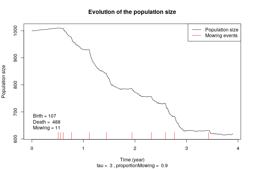
Figure 2 illustrates the evolution of the population size (number of crowns) of one trajectory of the model, for given parameters of the plant dynamics and management parameters. The initial population size was set to 1000, the mean number of mowing events a year $\tau=3$, the management project duration $T=4$ years and the proportion of mown crowns $proportionMowing=0.9$. We thus have a mean number of mowing events equal to $3\times 4=12$ (there were 11 in the simulation). The final population size is equal to 619, so the management strategy leads to a reduction of roughly one third in population size.

Figure 2: Simulation of one trajectory of the model (Equation (8)) with $\tau=3$, initial population size = 1000, $T=4$ and $proportionMowing=0.9$ with plant dynamics parameters from Table 1. Black line shows the population size, red lines indicate dates of mowing events.

2.4 Data for the Calibration

Our goal is to find the influence of management parameters on the stand dynamics. We must therefore set parameters of the plant dynamics. For some of the parameters, we could not find values in the literature. We thus proceed to a calibration which consists in finding parameter values of the plant dynamics with which the model best reproduces field data.

The field data are those used by Martin et al. (2018). The authors studied the invasion potential of the Japanese knotweed along an elevational gradient (i.e. in mountains), by identifying the determinants of its spatial dynamics. The experiment consists in collecting data on stands of Japanese knotweed at different altitudes in the French Alps. The measurements were carried out in 2008 and 2015, on the stands themselves (outline, stem density,…) as well as on biotic and abiotic variables. Stands were mown or not, and for each stand, we have access to some information about the management technique used by the land owner: the frequency of mowing and an estimation of the proportion of the mown stand, which corresponds to the side management technique. There is a high variability in the observed stands, both in size (from less than $2m^{2}$ to $350m^{2}$) and land conditions in which they grow such as soil quality, proximity of river, road, forest, abandoned land.

In model outputs, we compute the final and initial population sizes and areas (the area of the stand is the area of the convex hull formed around the simulated stands). From Martin et al. (2018), we use data about stand areas and crown densities so we can deduce the population size, for stands in 2008 and 2015.

As mentioned in B, the simulation operation for a stand takes place in two stages: first, the creation of the initial population given a population size to reach (we choose the size of a stand in 2008), then its evolution, according to the information related to management techniques contained in data from Martin et al. (2018).

2.5 The method used for the calibration

When we consider a set of parameters for the plant, and perform a simulation for each of the 19 stands, we obtain $19\times 4$ results (real numbers): the areas and sizes of the initial and final populations. We can thus compare these values with the $19\times 4$ corresponding observations of Martin et al. (2018). The goal is to find a set of parameters for the plant, common to all stands, that best matches the model outputs (area and size) to field observations. Notice that there is in particular the comparison between the initial size of the observations of 2008 and the one that has been simulated. This comparison is mainly used to check if the set of parameters of the plant being tested makes it possible to obtain an initial population. Indeed, some sets of parameters can lead to a failure in the creation of populations (e.g. if the distance of competition is too large whereas the dispersal distance is too small).

We thus need a distance to compare the simulations and the observations. We have chosen here, for each stand and each type (area or size), the distance: $dist(simu,data)=abs(simu-data)/data$. We have chosen to use a relative error distance (renormalization by the data) because areas and sizes have not the same order of magnitude, and there is also a wide difference within size values and area values themselves. The total distance to minimize is the sum of the distances over the 19 stands and over the 4 observations (size and area, in 2008 and 2015). Notice that if the set of parameters does not allow for the creation of an initial population, we obtain a population of size zero and a null area at the initial time (2008), and the simulated values for 2015 are also null. The distance between the observations and a trivial (null) population is equal to $76=(19\times 4)$.

In order to minimize this distance, the OpenMOLE software proposes a method based on genetic algorithms for model calibration (NSGA2). The result obtained is presented in Section 3.1. The calibration algorithm is an iterative algorithm, which provides at each step a set of solutions. As steps go by, the distance $dist(simu,data)$ between data and simulation results for the selected solutions decreases.

2.6 Numerical analysis

Simulations studied in the following are performed with the set of parameters for the plant dynamics obtained by calibration (Section 3.1, Table 1).

Let us now explain how we studied the influence of the management parameters $\tau$ and $T$ and of the initial population size, where we recall that

• $\tau$ is the mean number of mowing events a year

• $T$ is the duration of the project

We focus on the influence of these three parameters and we do not study the influence of the $proportionMowing$ parameter. We set its value to $0.9$ and use the random management technique. Indeed, we consider that the manager aims at mowing the whole stand, but we do not use a value of $proportionMowing$ equal to one in order to consider an imperfect mowing due to the tool used (as mentioned in Section 2.1).

We perform samplings of management parameters in OpenMOLE, with a replication of size n=50 for each set of management parameters (these samplings are detailed in Section 3.2) and we calculate the mean quantities over these $n$ values. Indeed, with our management point of view, we are interested in the mean behaviour of a stand. We first let one parameter vary. Based on an initial visual inspection of simulation results, we fit three relationships via least squares: a linear regression performed with $R$ function lm, a truncated quadratic relationship (Equation (10)), and an exponential regression (Equation (9)) performed with $R$ function nls. We assess model performance by the coefficient of determination ($R^{2}$) and the root mean squared errors (RMSE). Finally, in Section 3.2.4, we use the same statistical tools (lm and nls) to derive general regression formulas for the mean output quantities depending on management parameters, and two constants that the algorithm aims to find.

3 Results

3.1 Calibration

The values of calibrated parameters are presented in Table 1.

The set of solutions provided by the NSGA2 algorithm stabilized after 165000 steps. For a set of parameters, evol.sample refers to the number of replications that were carried out by the algorithm. Since our model is stochastic, we need to choose a solution with a sufficiently large value for evol.sample. Among the set of solutions provided by the algorithm, we chose the solution that was replicated at least 50 times, and that minimizes the distance $dist(simu,data)$.

Variable	Value after calibration	unit
K	12.72	g
L	0.26	$year^{-1}$
distanceCompetition	0.15	m
distanceParent	0.20	m
shape	4.34
scale	2.36
deathParameterDecrease	2.32	$g^{-1}$
deathParameterScaling	1.12	$year^{-1}$
mowingParameter	0.11	$g^{-1}$
bbar	0.18	$year^{-1}$
a0	1.73	g
score	26.06
evolution.samples	79

Table 1: Result of the calibration obtained with OpenMole software (Reuillon et al., 2013)

In Table 1, $score$ is the median over the 79 replications of the sum of the distances $dist(simu,data)$ over the 19 stands and the 4 characteristics (initial or final and area or size). A score of 26.06 means that in half of the cases and on average, the relative distance for one characteristic between the simulated stand and the corresponding data is lower than 0.3. The reason for this difference is that data were obtained from field work that was not carried out in order to calibrate the model, and thus contain a bias due to the altitude or soil type.

Even though we could not find values for the plant dynamics parameters in the literature, experts can provide boundaries for some of them. Thus, we can assess the ecological quality of the result given by the algorithm. First, the parameters $distanceCompetition$ and $distanceParent$ are close to what is expected according to our field experience. Then the distribution for the dispersal of individuals is close to the one suggested by specialists (Figure A.3). In Figure A.4, we plot the mortality rate of a crown according to its biomass. We note that a crown that is not mown keeps a very low mortality rate, in agreement with field observations. Indeed, to compare with the value in Smith et al. (2007), we calculate with Equation (6) and the parameter values from calibration, the probability that a crown dies before 4 months. This quantity is equal to 0.0027, which has the same order of magnitude as the value found in Smith et al. (2007) for the probability of a rhizome segment dying in a four months period (0.0083).

Finally, the ratio between the value of $K$ (maximal biomass, that is likely to be found for the oldest crown, i.e. in the center of the stand when there is no mowing), and $a_{0}$, the biomass of a crown at birth (rather in periphery) equals 7.4 (the ratio is expected to be around 10 in Adachi et al. (1996)).

3.2 Influence of management parameters and initial population size

In this section, the aim is to find statistical relationships between the explanatory variables (management parameters or the initial population size) and model outputs (mean area and mean size of a stand).

We consider the two following samplings:

• In $sampling1$, we make $\tau$ vary in $[0,15]$ in steps of 0.5, $T$ in $[0,16]$ in steps of 1 and $initialPopSize$ equals either 500 or 1500. We run 50 simulations of our stochastic model for each of these sets of values. $sampling1$ has a high sampling rate on $\tau$ and $T$, with high values for the initial population size. It is used in Sections 3.2.1 and 3.2.2 to study more precisely these two management parameters.

• In $sampling2$, we make $\tau$ vary in $[0,14]$ in steps of 2, $T$ in $[0,16]$ in steps of 2 and $initialPopSize$ in $[50,1200]$ in steps of 50. We run 50 simulations of our stochastic model for each of these sets of values. $sampling2$ has a high sampling rate on the initial population size, it is used in Section 3.2.3 to study more precisely its influence.

3.2.1 Influence of management duration $T$

In this section, we use the first sampling ($sampling1$) to study the influence of the management duration $T$ on the final mean areas and sizes. Given $\tau$ and a value of the initial population size, we perform

• a truncated quadratic regression for the mean final area.

• a non linear regression on strictly positive values for the mean final population size, using the function $f(T)=InitialPopSize*exp(-T/rate)$, with $rate$ being a constant on which the algorithm nls maximizes $R^{2}$. This constant rate is different for each set of parameters, since it depends on the values of $\tau$ and $initialPopSize$. In Section 3.2.4, we study this dependency.

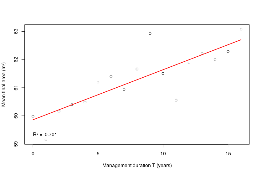
It turns out that for values of $\tau\leq 2.5$, the mean area remains close to its initial value at time $T=0$ (a maximum relative difference of $3m^{2}$), and the variation is rather linear but the corresponding $R^{2}$ values are below 0.9. Figure 3 gives an example of the linear regression on the mean area according to $T$, for given values of $\tau\leq 2.5$ and initial population size.

Figure 3: Linear regression of mean final area as a function of management duration $T$, with $\tau=0.5~{}year^{-1}$ and initial population size = 1500.

$R^{2}$ and RMSE values enable us to conclude that the mean final area depends quadratically on the management duration $T$ when $\tau>2.5$. Indeed, 47 regressions out of the 50 in the sampling (variation of initial Population size and $\tau>2.5$) lead to an $R^{2}$ value larger than 0.95. The maximal value of RMSE over these 50 regressions is 1.31 $m^{2}$, which is low compared to the mean initial area which has values 20 $m^{2}$ or 60 $m^{2}$. Figure 4 gives an example of the quadratic regression on the mean area for given values of $\tau$ and initial population size.

Figure 4: Quadratic regression of mean final area as a function of management duration $T$, with $\tau=8~{}year^{-1}$ and initial population size = 500. For the last three points in the bottom right hand corner, at least half of the 50 simulations lead to extinction.

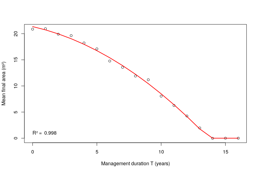
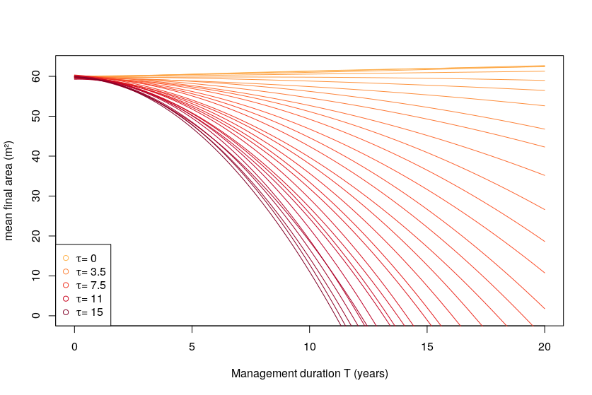
These results give information about the influence of the duration of the management project on stand growth. A first fact, which is very important for management is that it is not sufficient to mow to decrease the population size and area: if the number of mowings per year is too low (less than 2.5 in our case), the population size and area increase during the management project. In Figure 5, we plot the quadratic regression curves for the average final area with respect to the duration of the management project ($T$, on the abscissa), obtained for different $\tau$. A second important fact for management is that we cannot expect an eradication of a knotweed stand of initial area $60$ $m^{2}$ in less than 11 years (for 15 mowing events a year). The figure also tells us about the stand surface reduction in terms of final mean area when mowing once more time per year. For example, mowing 6 times a year instead of 5, during 10 years, reduces the final surface of the stand by $4$ $m^{2}$ on average (looking at the section $T=10$ on Figure 5).

Figure 5: Quadratic regression curves of the mean final area as a function of $T$, for different values of $\tau$ (low in clear colours, up to 15 mowings per year in dark colours), and we set $InitialPopSize=1500$ and $proportionMowing=0.9$.

As for the area, the size varies linearly for values of $\tau\leq 2.5$ ($R^{2}$ around 0.9). For larger values of $\tau$, we present here the result of the non linear regression.

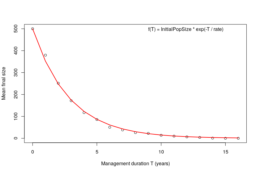
$R^{2}$ and RMSE values enable us to conclude that the mean final size depends exponentially on the management duration project $T$, when $\tau>2.5$. Indeed, all the 50 regressions in the sampling (variation of initial Population size and $\tau>2.5$) lead to an $R^{2}$ value larger than 0.95. The maximal value of RMSE over these 50 regressions is 39 crowns, which is low compared to the initial population size which has values 500 crowns or 1500 crowns.

Figure 6 gives an example of the quadratic regression on the mean area for given values of $\tau$ and initial population size.

Figure 6: Non linear regression of mean final size as a function of management duration project $T$ with $\tau=8~{}years^{-1}$ and initial population size = 500. For the last three points in the bottom right hand corner, at least half of the 50 simulations lead to extinction.

3.2.2 Influence of the mean number of mowing events a year $\tau$

In this section, we use the first sampling ($sampling1$) to study the influence of the mean number of mowing events a year on the final mean areas and sizes. Given a value of initial population size and $T$, we perform

• a linear regression on strictly positive values of outputs for the mean area.

• a non linear regression on strictly positive values for the mean final population size, using the function $f(\tau)=InitialPopSize*exp(-\tau/rate)$, with $rate$ being a constant on which the algorithm nls minimizes the sum of squared errors. This constant rate differs for each set of parameters since it depends on the values of $T$ and $initialPopSize$. As mentioned for the similar constant in Section 3.2.1, we study this dependency in Section 3.2.4.

The linear regression presented below holds for $\tau>2.5$ (as in Section 3.2.1) and $T\geq 2$ (to have a decreasing population).

$R^{2}$ and RMSE values enable us to conclude that the mean final area depends linearly on the mean number of mowing events $\tau$. Indeed, 24 regressions over the 30 in the sampling (variation of initial Population size and $T\geq 2$) lead to an $R^{2}$ value larger than 0.95. The maximal value of RMSE over these 50 regressions is $2.09$ $m^{2}$, which is low compared to the mean initial area which has values 20 $m^{2}$ or 60 $m^{2}$.

We also conclude that the mean final size depends exponentially on the mean number of mowing events $\tau$. Indeed, all the 30 regressions in the sampling (variation of initial Population size and $T\geq 2$) lead to an $R^{2}$ value larger than 0.95. The maximal value of RMSE over these 50 regressions is 64 crowns, which is low compared to the initial population size which has values 500 crowns or 1500 crowns.

3.2.3 Influence of the initial population size

In this section, we use the second sampling ($sampling2$) to study the influence of the initial population size on the final mean areas and sizes. Given a value for $\tau$ and $T$, we perform a linear regression on strictly positive values of outputs. Due to the wide range of values for the initial population size in the $sampling2$, too many extinctions may occur for a given set of management parameters. We thus perform the regression only if there are at least 5 strictly positive output values.

$R^{2}$ and RMSE values enable us to conclude that both the mean final area and the mean final size depend linearly on initial population size. Indeed, in both cases, 60 regressions over the 63 regressions among the 72 management sets in the sampling lead to an $R^{2}$ value larger than 0.95. The maximal value of RMSE over these 63 regressions is $1.1$ $m^{2}$ (resp. 18 crowns) for the mean final area (resp. the mean final size) case, which is low compared to the mean initial area (resp. initial population size) which ranges from 2 $m^{2}$ to 48 $m^{2}$ (resp. from 50 crowns to 1200 crowns).

Notice that the influence of the initial population size on the initial area is also linear. Indeed, the $sampling2$ contains the case $T=0$, and for this specific value of $T$ the final area is the initial area.

3.2.4 Formulas for the mean final sizes and areas, as functions of $\tau$, $T$ and the initial population size

We summarize results of the regressions we performed in Table 2.

Parameter	mean output	Variation	$R^{2}$ > 0.95	RMSE
$T$    for $\tau\geq 2.5$	final area	quadratic $\searrow$	47/50	1.31
$T$    for $\tau\geq 2.5$	final size	exponential $\searrow$	50/50	39
$\tau$     for $\tau\geq 2.5$	final area	linear $\searrow$	24/30	2.09
$\tau$     for $\tau\geq 2.5$	final size	exponential $\searrow$	30/30	64
$InitialPopSize$	final area	linear $\nearrow$	60/63	1.1
$InitialPopSize$	final size	linear $\nearrow$	60/63	18

Table 2: Summary of the regression results of Sections 3.2.1-3.2.3.

In Sections 3.2.1 to 3.2.3, we have studied the influence of one parameter, while the two others were set constant. The two previous samplings introduced at the very beginning of this Section 3.2 were designed to control the variation of management parameters and initial population size, in order to investigate their influence on the model outputs. Based on results in Sections 3.2.1 to 3.2.3, we are now able to propose a formula for the mean areas and sizes as a function of the two management parameters (the mean number of mowing events a year ($\tau$) and the management project duration ($T$)) and the initial population size. We use a Sobol sampling (that maximizes discrepancy of the sequence, i.e. the space is evenly covered) of 5000 points with $\tau\in[0;15.0]$, $T\in[0;20]$, and $initialPopSize\in[100;1500]$.

For the same reason as before, we consider the case of $\tau\geq 2.5$. Equations (9) and (10) highlight relationships between final outputs, management parameters and initial population size.

$$Mean~{}Final~{}Size~{}=InitialPopSize\times exp(-T.(\tau-a)/b),$$ (9)

with $a,b\in\mathbb{R}$ constants, and

$$Mean~{}Final~{}Area~{}=\max((c\times\tau+d)\times T^{2}+0.04\times InitialPopSize,0)$$ (10)

with $c,d\in\mathbb{R}$ constants.

We now discuss the results of the non linear regression with respect to the two management parameters ($T$ and $\tau>2$) and initial population size (the sampling contains 4332 values for the triplet ($T$, $\tau$, $InitialPopSize$)). $R^{2}$ and RMSE between the predicted values and the data for the mean size are respectively equal to 0.99 and 26.12 crowns. 95 % confidence intervals for the constants $a$ and $b$ are given by R and their values are: $a\in[0.90;0.94]$ and $b\in[20.46;20.77]$. $R^{2}$ and RMSE between the predicted values and the data for the mean area are respectively equal to 0.99 and 2.23 $m^{2}$. Moreover, the corresponding 95 % confidence intervals for the constants $c$ and $d$ are $c\in[-0.0342;-0.0336]$ and $d\in[0.0960;0.0998]$, respectively. Taking $T=0$ in the right hand side of Equations (9) and (10), gives $InitialPopSize$ and $InitialPopSize*0.04$, respectively. The last quantity thus corresponds to the mean initial area. There is indeed a linear dependency between the mean initial area and the initial population size.

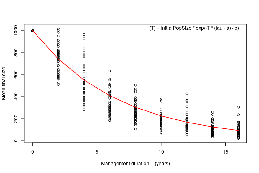
An important remark on the generality of Equations (9) and (10) is the following: results obtained for the mean output quantities are still relevant for direct outputs, without considering mean quantities. Figure 7 illustrates this point, plotting the formula (9), for given values of $\tau$ and initial population size and by letting $T$ vary. We emphasize that the red line on Figure 7 has been found with a regression on a far larger set of points than the subset selected to plot this example.

Figure 7: Exponential regression for the mean final size as a function of the management duration project ($T$). The red line is the prediction function of $T$ defined by Equation (9). Black circles represent stand sizes resulting of 50 replications with $\tau=4$, initial population size = 1000, letting $T$ vary.

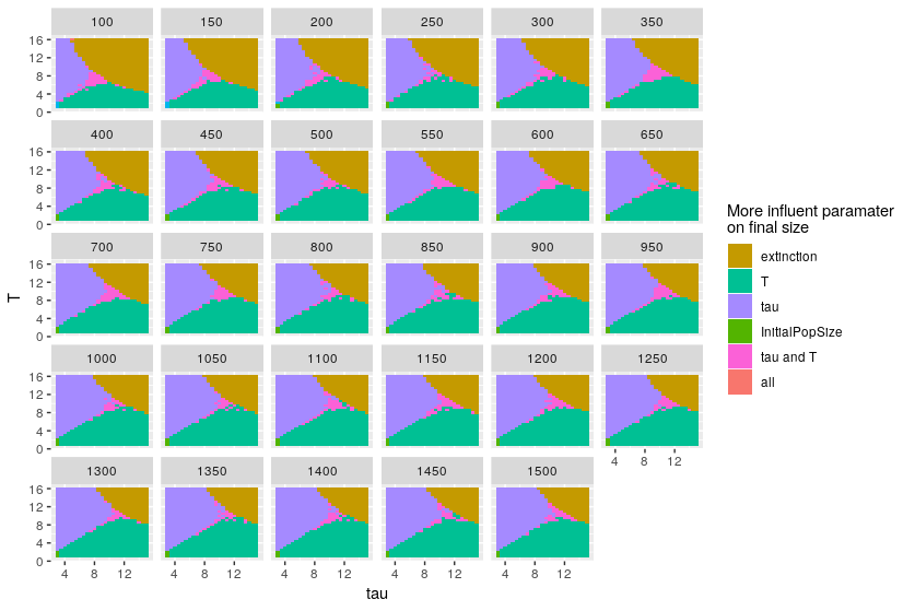
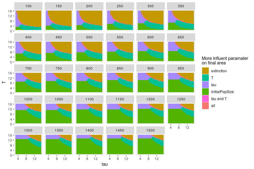
Equations (9) and (10) enable us to find which parameter most influences model outputs, and thus on which one it is better to concentrate management efforts. To do so, we compared for each value of the triplet ($T$,$\tau$,$InitialPopSize$) the final size and area according to Equations (9) and (10), for the three following parameter value combinations: ($T+1$,$\tau$,$InitialPopSize$), ($T$,$\tau+1$,$InitialPopSize$) and ($T$,$\tau$,$InitialPopSize\times 0.9$). Each plot on Figures 8 and 9 corresponds to a fixed value of $InitialPopSize$, with $\tau$ varying on the $x$-axis and $T$ varying on the $y$-axis, and associates with each triplet the most important parameter in a management perspective, that is the parameter the modification of which produces the lowest output (it happens that two modifications produce the lowest output). Brown zones correspond to set of parameter values that lead to eradication, thus in this zone no gain can be expected by any modification. Figure 8 shows that, out of the extinction zones, $T$ or $\tau$ have the greatest influence on final size and allows to determine the most efficient management modification. Especially, when $\tau$ is low, it is more efficient in terms of size reduction to mow one more time each year, and conversely, when $T$ is low, it is more efficient to continue mowing one more year. As for the final area, we observe on Figure 9 that areas corresponding to a greatest influence of $T$ or $\tau$ are reduced compared to Figure 8, in the favor of the area of greatest influence of $InitialPopSize$. In these regions of parameter values, beginning the management project on smaller stands (size equal to 90% of reference size) has more impact on the final area than mowing one more time each year or over a one year longer period of time; thus in these conditions, early detection of stands should be encouraged.

Figure 8: Parameters having the greatest influence on final size. Each plot corresponds to a fixed value of $InitialPopSize$ specified above the plots (from 100 to 1500 crowns), $\tau$ varies on the $x$-axis, and $T$ varies on the $y$-axis.

Figure 9: Parameters having the greatest influence on final area. Each plot corresponds to a fixed value of $InitialPopSize$ specified above the plots (from 100 to 1500 crowns), $\tau$ varies on the $x$-axis, and $T$ varies on the $y$-axis.

4 Discussion

In this paper, we proposed a stochastic individual based model for the growth of a stand of Japanese knotweed including mowing as a management technique. Then, we calibrated plant dynamics parameters with field data in Section 3.1. The set of parameters obtained was in agreement with values of parameters available in the literature and with our field experience. In Sections 3.2.1 - 3.2.3 we studied the influence of the initial population size, the mean number of mowing events a year and the management project duration on mean area and mean size of stands. We also obtained formulas for the area and size of a knotweed stand, as functions of those management parameters (for $\tau>2.5$) and initial population size. We have shown that mowing is not sufficient to decrease the population size and area. Indeed, if the number of mowing events per year is too small (smaller than 2.5 in our case), the population size and area increase during the management project. We have also shown how those results could be used by managers. Simulation results suggest the minimal duration of the management project necessary to achieve eradication (if it is possible at all, given a certain frequency of mowing). In Figure 5, we plotted the quadratic regression curves for the average final area with respect to the duration of the management project ($T$), obtained for different values of $\tau$ and for given values of $InitialPopSize$ and $proportionMowing$. The figure indicates the potential benefit in terms of invaded area reduction, of mowing the stand once more each year. More generally, formulas given in Equations (9) and (10), highlighting the relation between final outputs, management parameters and initial population size, enable to answer questions about the efficiency of different mowing strategies.

Following Dauer and Jongejans (2013) and Smith et al. (2007), we have assumed that the invasion occurs in an homogeneous area. Models that take into account the inhomogeneities of the invaded land are often static models, which do not consider the invasion as a dynamic phenomenon (no temporal component (Lookingbill et al., 2014; Buchadas et al., 2017)). Lookingbill et al. (2014) use indices such as habitat suitability, constructed from field data such as humidity or soil type, to produce invasibility maps. These maps assign a score to each zone which describes its probability of being invaded.

Another simplification in our model is that we did not take into account the dispersal of fragments of rhizome due to mowing. This may however be an important way of propagation of the plant in some conditions and it contributes to its invasiveness (Sásik and Eliás, 2006). Dispersal has to be considered if one wants to model the invasion of Japanese knotweed at the scale of a region composed of several stands. This will be the subject of future work. We could formulate this problem in the formalism of the viability theory (Aubin, 1991). In this framework, the dynamics of the system depends on the system state and on controls. One objective is to prove the existence of controls and to find initial values of the system such that the system state remains in a set of constraints (e.g. the invaded area below a given threshold). For example, managers could be interested in controlling the density of Japanese knotweed. Then we could study the resilience of the system, that is to say its ability to recover a property after a perturbation.

The importance of integration (biomass transfer between crowns) is still under debate. In Price et al. (2002), the authors notice that there is relatively few integration, whereas in Suzuki (1994) the authors found a larger integration. We did not consider this process in our model. Adding this phenomenon could produce simulation results closer to reality.

The field data we have used for the calibration were extracted from Martin et al. (2018). The measurements were carried out in 2008 and 2015 on stands that were mown or not. For each stand, data provide some information about the management technique used by the land owner: the frequency of mowing and an estimation of the proportion of the mown stand. Calibration results for some of the plant dynamics parameters based on these measurements are in agreements with data found in the literature.

The model is written in the formalism of measure-valued stochastic processes. The tools we used here for the particular case of the management of a Japanese knotweed stand can be used in a more general context. In particular, we could apply this method to others invasive plants, like seed dispersal species. One could even allow individuals to move in such models. In Leman (2016), the author took into account the spatial motion in an individual-based stochastic population model. Furthermore, including sexual reproduction of individuals, as in Smadi et al. (2018), would also enable to consider animal invasive species, like mosquitoes (Juliano and Philip Lounibos, 2005) or feral cats (Baker and Bode, 2016).

Aknowledgements

This work was partially funded by Electricit De France (EDF) and we thank Laure Santoni and Agnes Bariller for helpful discussions and comments. FL, SM and CS acknowledge partial funding from the Chair "Mod lisation Math matique et Biodiversit " of VEOLIA-Ecole Polytechnique-MNHN-F.X. FL and BR also acknowledge partial funding through the ANR "Alien" project (ANR 14-CE36-0001-01). Finally, IA, FL, SM and CS acknowledge Complex System Institute of Paris le de France for the hosting, and the OpenMOLE team for their advice on the software.

Appendix A Summary of model parameters

Table A.1 focuses on the plant dynamic parameters. We precise parameters units for those that have a biological meaning.

Variable	Description	unit
Biomass
$K$	maximal biomass (Equation (5))	g
$L$	biomass growth rate for low biomass (Equation (5))	$year^{-1}$
$a_{0}$	initial biomass (of a crown at birth)	g
Mowing
$mowingParameter$	in the mowing effect function in Equation (3)	$g^{-1}$
Mortality
$deathParameterScaling$	mortality rate for the low biomasses in Equation (7)	$year^{-1}$
$deathParameterDecrease$	decay rate of mortality function in Equation (7)	$g^{-1}$
Birth
$distanceParent$	apical dominance distance (Equation (1))	m
$distanceCompetition$	intraspecific competition distance (Equation (2))	g
$\bar{b}$	birth rate (under ideal conditions)	$year^{-1}$
$(\text{shape},\text{scale})$	Gamma law, dispersion of the new individual

Table A.1: Summary of model parameters

We have the following management parameters:

• mean number of mowing events a year: $\tau$

• management project duration: $T$

• proportion of mown crowns: $proportionMowing$

and initial population size parameter: $InitialPopSize$.

Appendix B Description of the algorithm used to simulate a solution of Equation (8).

We present one step of the algorithm that enables to make evolve a stand under mowing.

At each time, there are three possible events: a birth, a death or the mowing of a proportion $proportionMowing$ of individuals in the population. Suppose we have $N$ individuals at a time $t$. We start by calculating the next time at which there is an event, which requires the sum of the rates of the events of birth, death and mowing). The law of this time only depends on the current population state as the process is Markovian.

If it is a birth event, we select the parent uniformly at random in the population. We check whether the individual selected to be the parent does not already have too many neighbours at a distance lower than $distanceParent$. If it occurs, we draw the position of the new individual (child) according to the Gamma law described in the paragraph "Dispersal of the created individual" of Section 2.1 (with an angle chosen uniformly around the potential parent). If the child’s position falls into the set $C$ of Equation (2) (i.e. it does not fall into an intraspecific competition zone), then the individual is born at this position, and the new population size is $N+1$. Otherwise, i.e. if the parent has already enough crowns close to it, or if the new individual to be born is out of the set $C$, then there is no birth, and the population size remains $N$.

If the event is a mowing event, then we mow every individual with probability $proportionMowing$: we replace its biomass $a$ by $a*F(a)$.

Finally, if the event is a death event, then the individual likely to die is drawn uniformly at random, and we choose with the realization of a random variable whether this individual really dies according to its mortality rate, which depends on its biomass. If it dies, it is taken out of the population and the new population size is $N-1$, otherwise, nothing happens.

Between each event, the biomass of each individual grows in a deterministic way. The algorithm stops as soon as there is no more individual in the population.

For the simulations, we have to specify an initial population (at time 0, positions and biomass) that will evolve. To create an initial population, we use the algorithm above with initially one individual until the population reaches a prescribed size, with a low management technique ($\tau=1$ and $proportionMowing=0.9$). Indeed, if we put a larger value of $\tau$, we cannot often create the initial population because the original individual dies before producing offspring. In this spirit, we also let several attempts in the algorithm to create the initial population.

Appendix C Plots of functions defined in Section 2.1 with plant dynamics parameters from the calibration

Figure A.1: Function for the effect of mowing, Equation (3) with parameter values from the calibration (Table 1).

Figure A.2: Evolution of biomass, without mowing event, during 20 years (Equation (5)) with parameter values from the calibration (Table 1).

Figure A.3: Gamma law for the distance of dispersion with parameters values from the calibration (Table 1).

Figure A.4: Mortality rate, function of biomass (Equation (7)) with parameters values from the calibration (Table 1).

References

- Abgrall et al. (2018) Abgrall, C., Forey, E., Mignot, L., Chauvat, M., 2018. Invasion by fallopia japonica alters soil food webs through secondary metabolites. Soil Biology and Biochemistry 127, 100–109.
- Adachi et al. (1996) Adachi, I., Naoki, T., Terashima, M., 1996. Central die-back of monoclonal stands of Reynoutria Japonica in an early stage of primary succession on mount fuji. Annals of Botany 77, 477–486.
- Alberternst and Böhmer (2006) Alberternst, B., Böhmer, H., 2006. Invasive alien species fact sheet- fallopia japonica-. online database of the north european and baltic network on invasive alien species-nobanis. www. nobanis. org .
- Aubin (1991) Aubin, J.P., 1991. Viability theory. Springer Science & Business Media.
- Bailey and Wisskirchen (2006) Bailey, J., Wisskirchen, R., 2006. The distribution and origins of Fallopia Bohemica (polygonaceae) in europe. Nordic Journal of Botany 24, 173–199.
- Bailey et al. (2009) Bailey, J.P., Bímová, K., Mandák, B., 2009. Asexual spread versus sexual reproduction and evolution in japanese knotweed s.l. sets the stage for the "battle of the clones". Biological Invasions 11, 1189–1203.
- Baker and Bode (2016) Baker, C.M., Bode, M., 2016. Placing invasive species management in a spatiotemporal context. Ecological Applications 26, 712–725.
- Barney et al. (2006) Barney, J.N., Tharayil, N., DiTommaso, A., Bhowmik, P.C., 2006. The biology of invasive alien plants in canada. 5. Polygonum Cuspidatum sieb. & zucc.[= Fallopia Japonica (houtt.) Ronse Decr.]. Canadian Journal of Plant Science 86, 887–906.
- Bashtanova et al. (2009) Bashtanova, U.B., Beckett, K.P., Flowers, T.J., 2009. Physiological approaches to the improvement of chemical control of japanese knotweed (Fallopia Japonica). Weed science 57, 584–592.
- Beerling et al. (1994) Beerling, D.J., Bailey, J.P., Conolly, A.P., 1994. Fallopia Japonica (houtt.) Ronse Decraene. Journal of Ecology 82, 959–979.
- von Bertalanffy (1934) von Bertalanffy, L., 1934. Untersuchungen über die gesetzlichkeit des wachstums. Wilhelm Roux’Archiv für Entwicklungsmechanik der Organismen 131, 613–652.
- Bolker and Pacala (1997) Bolker, B., Pacala, S.W., 1997. Using moment equations to understand stochastically driven spatial pattern formation in ecological systems. Theoretical Population Biology 52, 179–197.
- Brock et al. (1992) Brock, J., Wade, M., et al., 1992. Regeneration of japanese knotweed (Fallopia Japonica) from rhizomes and stems: observation from greenhouse trials., in: IXe Colloque international sur la biologie des mauvaises herbes, 16-18 September 1992, Dijon, France., ANPP. pp. 85–94.
- Buchadas et al. (2017) Buchadas, A., Vaz, A.S., Honrado, J.P., Alagador, D., Bastos, R., Cabral, J.A., Santos, M., Vicente, J.R., 2017. Dynamic models in research and management of biological invasions. Journal of Environmental Management 196, 594–606.
- Champagnat (2006) Champagnat, N., 2006. A microscopic interpretation for adaptive dynamics trait substitution sequence models. Stochastic Processes and their Applications 116, 1127–1160.
- Champagnat et al. (2006) Champagnat, N., Ferrière, R., Méléard, S., 2006. Unifying evolutionary dynamics: from individual stochastic processes to macroscopic models. Theoretical Population Biology 69, 297–321.
- Colleran and Goodall (2014) Colleran, B.P., Goodall, K.E., 2014. In situ growth and rapid response management of flood-dispersed japanese knotweed (Fallopia Japonica). Invasive Plant Science and Management 7, 84–92.
- Coron et al. (2018) Coron, C., Costa, M., Leman, H., Smadi, C., 2018. A stochastic model for speciation by mating preferences. Journal of Mathematical Biology 76, 1421–1463.
- Costa et al. (2016) Costa, M., Hauzy, C., Loeuille, N., Méléard, S., 2016. Stochastic eco-evolutionary model of a prey-predator community. Journal of Mathematical Biology 72, 573–622.
- Dassonville et al. (2011) Dassonville, N., Guillaumaud, N., Piola, F., Meerts, P., Poly, F., 2011. Niche construction by the invasive asian knotweeds (species complex Fallopia): impact on activity, abundance and community structure of denitrifiers and nitrifiers. Biological Invasions 13, 1115–1133.
- Dauer and Jongejans (2013) Dauer, J.T., Jongejans, E., 2013. Elucidating the population dynamics of japanese knotweed using integral projection models. PloS one 8, e75181.
- De Waal (2001) De Waal, L., 2001. A viability study of Fallopia Japonica stem tissue. Weed Research 41, 447–460.
- Dieckmann et al. (2000) Dieckmann, U., Law, R., Metz, J.A., 2000. The geometry of ecological interactions: simplifying spatial complexity. Cambridge University Press.
- Dommanget et al. (2014) Dommanget, F., Evette, A., Spiegelberger, T., Gallet, C., Pace, M., Imbert, M., Navas, M.L., 2014. Differential allelopathic effects of japanese knotweed on willow and cottonwood cuttings used in riverbank restoration techniques. Journal of Environmental Management 132, 71–78.
- Fournier and Méléard (2004) Fournier, N., Méléard, S., 2004. A microscopic probabilistic description of a locally regulated population and macroscopic approximations. The Annals of Applied Probability 14, 1880–1919.
- Gerber et al. (2008) Gerber, E., Krebs, C., Murrell, C., Moretti, M., Rocklin, R., Schaffner, U., 2008. Exotic invasive knotweeds (Fallopia spp.) negatively affect native plant and invertebrate assemblages in european riparian habitats. Biological Conservation 141, 646–654.
- Gerber et al. (2010) Gerber, E., Murrell, C., Krebs, C., Bilat, J., Schaffner, U., 2010. Evaluating non-chemical management methods against invasive exotic knotweeds, Fallopia Spp. CABI, Egham .
- Gourley et al. (2016) Gourley, S.A., Li, J., Zou, X., 2016. A mathematical model for biocontrol of the invasive weed Fallopia Japonica. Bulletin of Mathematical Biology 78, 1678–1702.
- Gowton et al. (2016) Gowton, C., Budsock, A., Matlaga, D., 2016. Influence of disturbance on japanese knotweed (Fallopia Japonica) stem and rhizome fragment recruitment success within riparian forest understory. Natural Areas Journal 36, 259–267.
- Harris et al. (2009) Harris, C.M., Park, K.J., Atkinson, R., Edwards, C., Travis, J., 2009. Invasive species control: incorporating demographic data and seed dispersal into a management model for rhododendron ponticum. Ecological Informatics 4, 226–233.
- Juliano and Philip Lounibos (2005) Juliano, S.A., Philip Lounibos, L., 2005. Ecology of invasive mosquitoes: effects on resident species and on human health. Ecology Letters 8, 558–574.
- Kettunen et al. (2009) Kettunen, M., Genovesi, P., Gollasch, S., Pagad, S., Starfinger, U., ten Brink, P., Shine, C., 2009. Technical support to eu strategy on invasive alien species (ias). London: Institut for European Environnemental Policy (IEEP) .
- Kettunen et al. (2008) Kettunen, M., Genovesi, P., Gollasch, S., Pagad, S., Starfinger, U., Ten Brink, P., Shine, C., 2008. Technical support to eu strategy on invasive species (ias)-assessment of the impacts of ias in europe and the eu (final module report for the european commission) .
- Lavoie (2017) Lavoie, C., 2017. The impact of invasive knotweed species (Reynoutria spp.) on the environment: review and research perspectives. Biological Invasions 19, 2319–2337.
- Leman (2016) Leman, H., 2016. Convergence of an infinite dimensional stochastic process to a spatially structured trait substitution sequence. Stochastics and Partial Differential Equations: Analysis and Computations 4, 791–826.
- Lookingbill et al. (2014) Lookingbill, T.R., Minor, E.S., Bukach, N., Ferrari, J.R., Wainger, L.A., 2014. Incorporating risk of reinvasion to prioritize sites for invasive species management. Natural Areas Journal 34, 268–281.
- Maerz et al. (2005) Maerz, J.C., Blossey, B., Nuzzo, V., 2005. Green frogs show reduced foraging success in habitats invaded by japanese knotweed. Biodiversity & Conservation 14, 2901–2911.
- Martin et al. (2018) Martin, F.M., Dommanget, F., Janssen, P., Spiegelberger, T., Viguier, C., Evette, A., 2018. Could knotweeds invade mountains in their introduced range? an analysis of patches dynamics along an elevational gradient. Alpine Botany .
- Meier et al. (2014) Meier, E.S., Dullinger, S., Zimmermann, N.E., Baumgartner, D., Gattringer, A., Hülber, K., 2014. Space matters when defining effective management for invasive plants. Diversity and Distributions 20, 1029–1043.
- Murphy and Romanuk (2014) Murphy, G.E., Romanuk, T.N., 2014. A meta-analysis of declines in local species richness from human disturbances. Ecology and Evolution 4, 91–103.
- Paine et al. (2012) Paine, C., Marthews, T.R., Vogt, D.R., Purves, D., Rees, M., Hector, A., Turnbull, L.A., 2012. How to fit nonlinear plant growth models and calculate growth rates: an update for ecologists. Methods in Ecology and Evolution 3, 245–256.
- Pimentel et al. (2005) Pimentel, D., Zuniga, R., Morrison, D., 2005. Update on the environmental and economic costs associated with alien-invasive species in the united states. Ecological Economics 52, 273–288.
- Price et al. (2002) Price, E.A., Gamble, R., Williams, G.G., Marshall, C., 2002. Seasonal patterns of partitioning and remobilization of 14c in the invasive rhizomatous perennial japanese knotweed (Fallopia Japonica (houtt.) RRonse Decraene). Ecology and Evolutionary Biology of Clonal Plants , 125–140.
- Pyšek and Richardson (2010) Pyšek, P., Richardson, D.M., 2010. Invasive species, environmental change and management, and health. Annual Review of Environment and Resources 35.
- Reuillon et al. (2013) Reuillon, R., Leclaire, M., Rey-Coyrehourcq, S., 2013. Openmole, a workflow engine specifically tailored for the distributed exploration of simulation models. Future Generation Computer Systems 29, 1981 – 1990. URL: http://www.openmole.org/files/FGCS2013.pdf.
- Rouifed et al. (2011) Rouifed, S., Bornette, G., Mistler, L., Piola, F., 2011. Contrasting response to clipping in the asian knotweeds Fallopia Japonica and Fallopia Bohemica. Ecoscience 18, 110–114.
- Saldaña et al. (2009) Saldaña, A., Fuentes, N., Pfanzelt, S., 2009. Fallopia Japonica (houtt.) Ronse Decraene. (polygonaceae), : A new record for the alien flora of chile. Gayana. Botánica 66, 283–285.
- Sásik and Eliás (2006) Sásik, R., Eliás, P., 2006. Rhizome regeneration of Fallopia Japonica (japanese knotweed)(houtt.) Ronse Decr. i. regeneration rate and size of regenerated plants. Folia Oecologica 33, 57.
- Seiger et al. (1997) Seiger, L.A., Merchant, H.C., et al., 1997. Mechanical control of japanese knotweed (Fallopia Japonica [houtt.] Ronse Decraene): Effects of cutting regime on rhizomatous reserves. Natural Areas Journal 17, 341–345.
- Serniak et al. (2017) Serniak, L.T., Corbin, C.E., Pitt, A.L., Rier, S.T., 2017. Effects of japanese knotweed on avian diversity and function in riparian habitats. Journal of Ornithology 158, 311–321.
- Shackleton et al. (2019) Shackleton, R.T., Shackleton, C.M., Kull, C.A., 2019. The role of invasive alien species in shaping local livelihoods and human well-being: A review. Journal of Environmental Management 229, 145–157.
- Siemens and Blossey (2007) Siemens, T.J., Blossey, B., 2007. An evaluation of mechanisms preventing growth and survival of two native species in invasive bohemian knotweed (Fallopia Bohemica, polygonaceae). American Journal of Botany 94, 776–783.
- Simberloff et al. (2013) Simberloff, D., Martin, J.L., Genovesi, P., Maris, V., Wardle, D.A., Aronson, J., Courchamp, F., Galil, B., García-Berthou, E., Pascal, M., et al., 2013. Impacts of biological invasions: what’s what and the way forward. Trends in Ecology & Evolution 28, 58–66.
- Smadi et al. (2018) Smadi, C., Leman, H., Llaurens, V., 2018. Looking for the right mate in diploid species: How does genetic dominance affect the spatial differentiation of a sexual trait? Journal of Theoretical Biology 447, 154–170.
- Smith et al. (2007) Smith, J., Ward, J.P., Child, L.E., Owen, M., 2007. A simulation model of rhizome networks for Fallopia Japonica (Japanese knotweed) in the united kingdom. Ecological Modelling 200, 421–432.
- Strayer (2012) Strayer, D.L., 2012. Eight questions about invasions and ecosystem functioning. Ecology Letters 15, 1199–1210.
- Suzuki (1994) Suzuki, J.I., 1994. Growth dynamics of shoot height and foliage structure of a rhizomatous perennial herb, Polygonum Cuspidatum. Annals of Botany 73, 629–638.
- Tharayil et al. (2013) Tharayil, N., Alpert, P., Bhowmik, P., Gerard, P., 2013. Phenolic inputs by invasive species could impart seasonal variations in nitrogen pools in the introduced soils: a case study with Polygonum Cuspidatum. Soil Biology and Biochemistry 57, 858–867.
- Tran (2006) Tran, V.C., 2006. Modèles particulaires stochastiques pour des problèmes d’évolution adaptative et pour l’approximation de solutions statistiques. Ph.D. thesis. Université de Nanterre-Paris X.
- Tran (2008) Tran, V.C., 2008. Large population limit and time behaviour of a stochastic particle model describing an age-structured population. ESAIM: Probability and Statistics 12, 345–386.
- Travis et al. (2011) Travis, J.M., Harris, C.M., Park, K.J., Bullock, J.M., 2011. Improving prediction and management of range expansions by combining analytical and individual-based modelling approaches. Methods in Ecology and Evolution 2, 477–488.
- Zeide (1993) Zeide, B., 1993. Analysis of growth equations. Forest science 39, 594–616.