There are No Bit Parts for Sign Bits in Black-Box Attacks

Abstract

We present a black-box adversarial attack algorithm which sets new state-of-the-art model evasion rates for query efficiency in the $\ell_{\infty}$ and $\ell_{2}$ metrics, where only loss-oracle access to the model is available. On two public black-box attack challenges, the algorithm achieves the highest evasion rate, surpassing all of the submitted attacks. Similar performance is observed on a model that is secure against substitute-model attacks. For standard models trained on the MNIST, CIFAR10, and IMAGENET datasets, averaged over the datasets and metrics, the algorithm is $3.8\times$ less failure-prone, and spends in total $2.5\times$ fewer queries than the current state-of-the-art attacks combined given a budget of $10,000$ queries per attack attempt. Notably, it requires no hyperparameter tuning or any data/time-dependent prior. The algorithm exploits a new approach, namely sign-based rather than magnitude-based gradient estimation. This shifts the estimation from continuous to binary black-box optimization. With three properties of the directional derivative, we examine three approaches to adversarial attacks. This yields a superior algorithm breaking a standard MNIST model using just 12 queries on average!

1 Introduction

Problem.

Deep Neural Networks (DNNs) are vulnerable to adversarial examples, which are malicious inputs designed to fool the network’s prediction—see (Biggio & Roli, 2018) for a comprehensive, recent overview of adversarial examples. Research on generating these malicious inputs started in the white-box setting, where access to the gradients of the models was assumed. Since the gradient points to the direction of steepest ascent, a malicious input can be perturbed along that gradient to maximize the network’s loss, thereby fooling its prediction. The assumption of access to the underlying gradient does not however reflect real world scenarios. Attacks accepting a more realistic, restrictive black-box threat model, which do not assume access to gradients, have since been studied as will be summarized shortly.

Central to the approach of generating adversarial examples in a black-box threat model is estimating the gradients of the model being attacked. In estimating these gradients (their magnitudes and signs), the community at large has focused on formulating it as a problem in continuous optimization. Their works seek to reduce the query complexity from the standard $O(n)$, where $n$ is the number of input features/covariates. In this paper, we take a different view and focus on estimating just the sign of the gradient by reformulating the problem as minimizing the Hamming distance to the gradient sign. Given access to a Hamming distance (to the gradient sign) oracle, this view guarantees a query complexity of $\Omega(n/\log_{2}(n+1))$: an order of magnitude lesser than the full gradient estimation’s query complexity for most practically-occurring input dimensions $n$. Our key objective is to answer the following: Is it possible to recover the sign of the gradient with high query efficiency and generate adversarial examples as effective as those generated by full gradient estimation approaches?

To this end, we propose a novel formulation capitalizing on some properties of the directional derivative which, approximated by finite difference of loss queries, has been the powerhouse of black-box attacks. Particularly, this leads to the following contributions at the intersection of adversarial machine learning and black-box (zeroth-order) optimization: 1) We present three properties of the directional derivative of the loss function of the model under attack in the direction of $\{\pm 1\}^{n}$ vectors, and propose methods to estimate the gradient sign bits exploiting these properties. Based on one of the properties, namely separability, we devise a divide-and-conquer algorithm, which we refer to as SignHunter, that reduces the search complexity from $2^{n}$ sign vectors to $O(n)$. When given a budget of $O(n)$ queries, SignHunter is guaranteed to perform at least as well as FGSM (Goodfellow et al., 2015), which has access to the model’s gradient. Through rigorous experiments on both standard and adversarially trained models, we find that SignHunter, in its search for the gradient sign, crafts adversarial examples within a fraction of this number of queries outperforming FGSM and other state-of-the-art black-box attacks. 2) We release a software framework to systematically benchmark adversarial black-box attacks on DNNs for MNIST, CIFAR10, and IMAGENET datasets in terms of their success rate, query count, and other related metrics. 3) We identify several key areas of research which we believe will help the community of adversarial learning and gradient-free optimization.

(a)	(b)	(c)

Figure 1: Misclassification rate of three neural nets (for (a) MNIST, (b) CIFAR10, and (c) IMAGENET) on the noisy FGSM’s adversarial examples as a function of correctly estimated coordinates of $\operatorname{sign}(\nabla_{\bm{x}}f(\bm{x},y))$ on random $1000$ images from the corresponding datasets. Across all the models, estimating the sign of the top $30\%$ gradient coordinates (in terms of their magnitudes) is enough to achieve a misclassification rate of $\sim 70\%$. More details can be found in Appendix A.

Related Work.

We organize the related work in two themes, namely Adversarial Example Generation and Sign-Based Optimization.

Adversarial Example Generation. This literature can be organized as generating examples in either a white-box or a black-box setting. Nelson et al. (2012) provide a theoretical framework to analyze adversarial querying in a white-box setting. Following the works of Biggio et al. (2013) and Goodfellow et al. (2015) who introduced the fast gradient sign method (FGSM), several methods to produce adversarial examples have been proposed for various learning tasks and threat perturbation constraints (Carlini & Wagner, 2017; Moosavi-Dezfooli et al., 2016; Hayes & Danezis, 2017; Al-Dujaili et al., 2018; Huang et al., 2018; Kurakin et al., 2017; Shamir et al., 2019). These methods assume a white-box setup and are not the focus of this work. An approach, which has received the community’s attention, involves learning adversarial examples for one model (with access to its gradient information) to transfer them against another (Liu et al., 2016; Papernot et al., 2017). As an alternative to the transferability phenomenon, Xiao et al. (2018) use a Generative Adversarial Network (GAN) to generate adversarial examples which are based on small norm-bounded perturbations. Both approaches involve learning on a different model, which is expensive, and does not lend itself to comparison in our setup, where we directly query the model of interest. Among works which generate examples in a black-box setting through iterative optimization schemes, Narodytska & Kasiviswanathan (2017) showed how a naïve policy of perturbing random segments of an image achieved adversarial example generation. They do not use any gradient information. Bhagoji et al. (2017) reduce the dimensions of the feature space using Principal Component Analysis (PCA) and random feature grouping, before estimating gradients. This enables them to bound the number of queries made. Chen et al. (2017) introduced a principled approach to solving this problem using gradient based optimization. They employ finite differences, a zeroth-order optimization tool, to estimate the gradient and then use it to design a gradient-based attack on models. While this approach successfully generates adversarial examples, it is expensive in the number of queries made to the model. Ilyas et al. (2018) substitute traditional finite differences methods with Natural Evolutionary Strategies (NES) to obtain an estimate of the gradient. Tu et al. (2018) provide an adaptive random gradient estimation algorithm that balances query counts and distortion, and introduces a trained auto-encoder to achieve attack acceleration. (Ilyas et al., 2019) extend this line of work by proposing the idea of gradient priors and bandits: Bandits_TD. Our work contrasts the general approach used by these works. We investigate whether just estimating the sign of the gradient suffices to efficiently generate examples.

Sign-Based Optimization. In the context of general-purpose continuous optimization methods, sign-based stochastic gradient descent was studied in both zeroth- and first-order setups. In the latter, Bernstein et al. (2018) analyzed signSGD, a sign-based Stochastic Gradient Descent, and showed that it enjoys a faster empirical convergence than SGD in addition to the cost reduction of communicating gradients across multiple workers. Liu et al. (2019) extended signSGD to zeroth-order setup with the ZO-SignSGD algorithm. ZO-SignSGD requires $\sqrt{n}$ times more iterations than signSGD, leading to a convergence rate of $O(\sqrt{n/T})$, where $n$ is the number of optimization variables, and $T$ is the number of iterations.

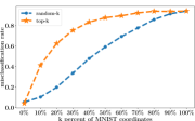
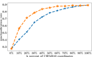
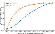
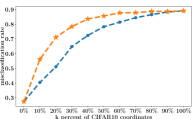
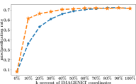
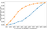
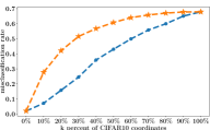
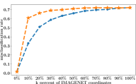
Adversarial Examples Meet Sign-based Optimization. In the context of adversarial examples generation, the effectiveness of sign of the gradient coordinates was noted in both white- and black-box settings. In the former, the Fast Gradient Sign Method (FGSM)—which is algorithmically similar to signSGD—was proposed to generate white-box adversarial examples (Goodfellow et al., 2015). Ilyas et al. (2019) examined a noisy version of FGSM to address the question of How accurate of a gradient estimate is necessary to execute a successful attack on a neural net. In Figure 1, we reproduce their experiment on an IMAGENET-based model—Plot (c)—and extended it to the MNIST and CIFAR10 datasets—Plots (a) and (b). Observe that estimating the sign of the top $30\%$ gradient coordinates (in terms of their magnitudes) is enough to achieve a misclassification rate of $\sim 70\%$. Furthermore, ZO-SignSGD (Liu et al., 2019) was shown to perform better than NES at generating adversarial examples against a black-box neural network on the MNIST dataset.

2 Formal Background

Notation.

Let $n$ denote the dimension of a neural network’s input. Denote a hidden $n$-dimensional binary code by $\bm{q}^{*}$. That is, $\bm{q}^{*}\in\mathcal{H}\equiv\{-1,+1\}^{n}$. The response of the Hamming (distance) oracle $\mathcal{O}$ to the $i$th query $\bm{q}^{(i)}\in\mathcal{H}$ is denoted by $r^{(i)}\in\{0,\ldots,n\}$ and equals the Hamming distance $r^{(i)}=||\bm{q}^{(i)}-\bm{q}^{*}||_{H}$, where the Hamming norm $||\bm{v}||_{H}$ is defined as the number of non-zero entries of vector $\bm{v}$. We also refer to $\mathcal{O}$ as the noiseless Hamming oracle, in contrast to the noisy Hamming oracle $\hat{\mathcal{O}}$, which returns noisy versions of $\mathcal{O}$’s responses. $\mathbf{1}_{n}$ is the $n$-dimensional vector of ones. The query ratio $\rho\in(0,1]$ is defined as $m/n$ where $m$ is the number of queries to $\mathcal{O}$ required to retrieve $\bm{q}^{*}$. Furthermore, denote the directional derivative of some function $f$ at a point $\bm{x}$ in the direction of a vector $\bm{v}$ by $D_{\bm{v}}f(\bm{x})\equiv\bm{v}^{T}\nabla_{\bm{x}}f(\bm{x})$ which often can be approximated by the finite difference method. That is, for $\delta>0$, we have

$$D_{\bm{v}}f(\bm{x})=\bm{v}^{T}\nabla_{\bm{x}}f(\bm{x})\approx\frac{f(\bm{x}+\delta\bm{v})-f(\bm{x})}{\delta}\;.$$ (1)

Let $\Pi_{S}(\cdot)$ be the projection operator onto the set $S$, $B_{p}(\bm{x},\epsilon)$ be the $\ell_{p}$ ball of radius $\epsilon$ around $\bm{x}$. Next, we provide lower and upper bounds on the query ratio $\rho$.

Bounds on the Query Ratio $\rho$.

Using a packing argument,  Vaishampayan (2012) proved the following lower bound on query ratio $\rho$.

Theorem 1.

(Vaishampayan, 2012, Theorem 1) For the noiseless Hamming oracle $\mathcal{O}$, the query ratio must satisfy $\rho=m/n\geq\frac{1}{\log_{2}(n+1)}$ for any sequence of $m$ queries that determine every $n$-dimensional binary code $\bm{q}^{*}$ uniquely.

Proof.

See (Vaishampayan, 2012, Page 4). ∎

In the following theorem, we show that no more than $n$ queries are required to retrieve the hidden $n$-dimensional binary code $\bm{q}^{*}$.

Theorem 2.

A hidden $n$-dimensional binary code $\bm{q}^{*}\in\mathcal{H}$ can be retrieved exactly with no more than $n$ queries to the noiseless Hamming oracle $\mathcal{O}$.

Proof.

See Appendix C. ∎

3 Gradient Estimation Problem

At the heart of black-box adversarial attacks is generating a perturbation vector to slightly modify the original input $\bm{x}$ so as to fool the network prediction of its true label $y$. Put differently, an adversarial example $\bm{x}^{\prime}$ maximizes the network’s loss $L(\bm{x}^{\prime},y)$ but still remains $\epsilon_{p}$-close to the original input $\bm{x}$. Although the loss function $L$ can be non-concave, gradient-based techniques are often very successful in crafting an adversarial example (Madry et al., 2017). That is, setting the perturbation vector as a step in the direction of $\nabla_{\bm{x}}L(\bm{x},y)$. Consequently, the bulk of black-box attack methods try to estimate the gradient by querying an oracle that returns, for a given input/label pair $(\bm{x},y)$, the value of the network’s loss $L(\bm{x},y)$. Using only such value queries, the basic approach relies on the finite difference method to approximate the directional derivative (Eq. 1) of the function $L$ at the input/label pair $(\bm{x},y)$ in the direction of a vector $\bm{v}$, which corresponds to $\bm{v}^{T}\nabla_{\bm{x}}L(\bm{x},y)$. With $n$ linearly independent vectors $\{{\bm{v}^{(i)}}^{T}\nabla_{\bm{x}}L(\bm{x},y)=d^{(i)}\}_{1\leq i\leq n}$, one can construct a linear system of equations to recover the full gradient. Clearly, this approach’s query complexity is $O(n)$, which can be prohibitively expensive for large $n$ (e.g., $n=268,203$ for the IMAGENET dataset). Moreover, the queries are not adaptive, whereas one could make use of the past queries’ responses to construct the new query and recover the full gradient with less queries. Recent works tried to mitigate this issue by exploiting data- and/or time-dependent priors (Tu et al., 2018; Ilyas et al., 2018, 2019).

The lower bound of Theorem 1 on the query complexity of a Hamming oracle $\mathcal{O}$ to find a hidden vector $\bm{q}^{*}$ suggests the following: instead of estimating the full gradient (sign and magnitude) and apart from exploiting any data- or time-dependent priors; focus on estimating its sign After all, simply leveraging (noisy) sign information of the gradient yields successful attacks; see Figure 1. Therefore, our interest in this paper is the gradient sign estimation problem, which we formally define next, breaking away from the full gradient estimation to construct black-box adversarial attacks.

Definition 1.

(Gradient Sign Estimation Problem) For an input/label pair $(\bm{x},y)$ and a loss function $L$, let $\bm{g}^{*}=\nabla_{\bm{x}}L(\bm{x},y)$ be the gradient of $L$ at $(\bm{x},y)$ and $\bm{q}^{*}=\operatorname{sign}(\bm{g}^{*})\in\mathcal{H}$ be the sign bit vector of $\bm{g}^{*}$. Then the goal of the gradient sign estimation problem is to find a binary vector $\bm{q}\in\mathcal{H}$ minimizing the Hamming norm

$$\min_{\bm{q}\in\mathcal{H}}\ ||\bm{q}-\bm{q}^{*}||_{H}\;,$$ (2)

or equivalently maximizing the directional derivative

$$\max_{\bm{q}\in\mathcal{H}}D_{\bm{q}}L(\bm{x},y)\;,$$ (3)

from a limited number of (possibly adaptive) function value queries $L(\bm{x}^{\prime},y)$.

Next, we tackle the gradient sign estimation problem leveraging three properties of the loss directional derivative $D_{\bm{q}}L(\bm{x},y)$ which, in the black-box setup, is approximated by finite difference of loss value queries $L(\bm{x}^{\prime},y)$.

4 A Framework for Estimating Sign of the Gradient from Loss Oracles

Our goal is to estimate the gradient sign bits of the loss function $L$ of the model under attack at an input/label pair ($\bm{x},y$) from a limited number of loss value queries $L(\bm{x}^{\prime},y)$. To this end, we examine the basic concept of directional derivatives that has been employed in recent black-box adversarial attacks. Particularly, we present three approaches to estimate the gradient sign bits based on three properties of the directional derivative $D_{\bm{q}}L(\bm{x},y)$ of the loss in the direction of a sign vector $\bm{q}\in\mathcal{H}$. For the rest of the paper, we only discuss the most successful one: Divide & Conquer. Others are described in Appendix B.

Approach 1: Divide & Conquer.

Based on the definition of the directional derivative (Eq. 1), we state the following property.

Property 1 (Separability of $D_{\bm{q}}L(\bm{x},y)$).

The directional derivative $D_{\bm{q}}L(\bm{x},y)$ of the loss function $L$ at an input/label pair $(\bm{x},y)$ in the direction of a binary code $\bm{q}$ is separable. That is,

$$\max_{\bm{q}\in\mathcal{H}}D_{\bm{q}}L(\bm{x},y)=\max_{\bm{q}\in\mathcal{H}}\bm{q}^{T}\bm{g}^{*}=\sum_{i=1}^{n}\max_{q_{i}\in\{-1,+1\}}q_{i}g^{*}_{i}$$ (4)

We employ the above property in a divide-and-conquer search which we refer to as SignHunter. As outlined in Algorithm 1, the technique starts with a random guess of the sign vector $\bm{q}_{1}$. It then proceeds to flip the sign of all the coordinates to get a new sign vector $\bm{q}_{2}$, and revert the flips if the loss oracle returned a value $L(\bm{x}+\delta\bm{q}_{2},y)$ (or equivalently the directional derivative ) less than the best obtained so far $L(\bm{x}+\delta\bm{q}_{1},y)$. SignHunter applies the same rule to the first half of the coordinates, the second half, the first quadrant, the second quadrant, and so on. For a search space of dimension $n$, SignHunter needs $2^{\lceil\log(n)+1\rceil}-1$ sign flips to complete its search. If the query budget is not exhausted by then, one can update $\bm{x}$ with the recovered signs and restart the procedure at the updated point with a new starting code $\bm{q}_{1}$ ($\bm{s}$ in Algorithm 1). In the next theorem, we show that SignHunter is guaranteed to perform at least as well as the Fast Gradient Sign Method FGSM with $O(n)$ oracle queries.

Theorem 3.

(Optimality of SignHunter) Given $2^{\lceil\log(n)+1\rceil}$ queries and that the directional derivative is well approximated by the finite-difference (Eq. 1), SignHunter is at least as effective as FGSM (Goodfellow et al., 2015) in crafting adversarial examples.

Proof.

See Appendix C. ∎

Theorem 3 provides an upper bound on the number of queries required for SignHunter to recover the gradient sign bits, and perform as well as FGSM. In practice (as will be shown in our experiments), SignHunter crafts adversarial examples with a fraction of this upper bound. Note that one could recover the gradient sign vector with $n+1<2^{\lceil\log(n)+1\rceil}$ queries by starting with an arbitrary sign vector and flipping its bits sequentially. Nevertheless, SignHunter incorporates its queries in a framework of majority voting (weighted by the magnitude of the gradient coordinates) to recover as many sign bits as possible with as few queries as possible. Consider the case where all the gradient coordinates have the same magnitude. If we start with a random sign vector whose Hamming distance to the optimal sign vector $\bm{q}^{*}$ is $n/2$: agreeing with $\bm{q}^{*}$ in the first half of coordinates. In this case, SignHunter needs just three queries to recover the entire sign vector, whereas the sequential bit flipping would require $n+1$ queries. While the magnitudes of gradient coordinates may not have the same value as considered in the previous example; through empirical evaluation (see Appendix G), we found them to be concentrated. Consequently and with high probability, their votes on retaining or reverting sign flips are weighted similarly.

Algorithm 1 SignHunter
Input:
$g:\mathcal{H}\to\operatorname{\mathbb{R}}$ : the black-box function to be maximized over the binary hypercube $\mathcal{H}\equiv\{-1,+1\}^{n}$

  def init$(g):$      $i\leftarrow 0$      $h\leftarrow 0$      $g\leftarrow g$      $\bm{s}\sim\mathcal{U}(\mathcal{H})$ // e.g., all ones $[+1,+1,\ldots,+1]$      done $\leftarrow false$      $g_{best}\leftarrow-\infty$

   def is_done$():$       return done

   def step$():$       chunk_len $\leftarrow\lceil n/2^{h}\rceil$        flip the bits of $\bm{s}$ indexed from $i*$chunk_len till          $(i+1)*$chunk_len       if $g(\bm{s})\geq g_{best}$:             $g_{best}\leftarrow g(\bm{s})$       else:             flip back the bits of $\bm{s}$ indexed from                 $i*$chunk_len till $(i+1)*$chunk_len       increment $i$       if $i==2^{h}$:             $i\leftarrow 0$              increment $h$             if $h==\lceil\log_{2}(n)\rceil+1$: done $\leftarrow true$

   def get_current_sign_estimate$():$       return $\bm{s}$

Algorithm 2 Black-Box Adversarial Example Generation with SignHunter
Input:

$\bm{x}_{init}$	: input to be perturbed,
$y_{init}$	: $\bm{x}_{init}$’s true label,
$B_{p}(.,\epsilon)$	: $\ell_{p}$ perturbation ball of radius $\epsilon$
$L$	: loss function of the neural net under attack

1:  $\delta\leftarrow\epsilon$ // set finite-difference probe to perturbation bound

2:  $\bm{x}_{o}\leftarrow\bm{x}_{init}\$

3:  Define the function $g$ as

$$g(\bm{q})=\frac{L(\Pi_{B_{p}(\bm{x}_{init},\epsilon)}(\bm{x}_{o}+\delta\bm{q}),y_{init})-L(\bm{x}_{o},y_{init})}{\delta}$$

4:  SignHunter.init$(g)$

5:  $//C(\cdot)$ returns top class

6:  while $C(\bm{x})=y_{init}$ do

7:    SignHunter.step()

8:    $\bm{s}\leftarrow$ SignHunter.get_current_sign_estimate()

9:    $\bm{x}\leftarrow\Pi_{B_{p}(\bm{x}_{init},\epsilon)}(\bm{x}_{o}+\delta\bm{s})$

10:    if SignHunter.is_done() then

11:       $\bm{x}_{o}\leftarrow\bm{x}$

12:       Define the function $g$ as

$$g(\bm{q})=\frac{L(\Pi_{B_{p}(\bm{x}_{init},\epsilon)}(\bm{x}_{o}+\delta\bm{q}),y_{init})-L(\bm{x}_{o},y_{init})}{\delta}$$

13:       SignHunter.init$(g)$

14:    end if

15:  end while

16:  return $\bm{x}$

Further, SignHunter is amenable to parallel hardware architecture and thus can carry out attacks in batches more efficiently, compared to the other two approaches we considered. We tested all the proposed approaches (SignHunter and those in Appendix B) on a set of toy problems and found that SignHunter perform significantly better. For these reasons, in our experiments on the real datasets MNIST, CIFAR10, IMAGENET; we opted for SignHunter as our algorithm of choice to estimate the gradient sign in crafting black-box adversarial attacks as outlined in Algorithm 2.

5 Experiments

We evaluate SignHunter and compare it with established algorithms from the literature: ZO-SignSGD (Liu et al., 2019), NES (Ilyas et al., 2018), and Bandits_TD (Ilyas et al., 2019) in terms of their effectiveness in crafting (without loss of generality) untargeted black-box adversarial examples. Both $\ell_{\infty}$ and $\ell_{2}$ threat models are considered on the MNIST, CIFAR10, and IMAGENET datasets.

Experiments Setup.

Our experiment setup is similar to (Ilyas et al., 2019). Each attacker is given a budget of $10,000$ oracle queries per attack attempt and is evaluated on $1000$ images from the test sets of MNIST, CIFAR10, and the validation set of IMAGENET. We did not find a standard practice of setting the perturbation bound $\epsilon$, arbitrary bounds were used in several papers.

We set the perturbation bounds based on the following. For the $\ell_{\infty}$ threat model, we use (Madry et al., 2017)’s bound for MNIST and (Ilyas et al., 2019)’s bounds for both CIFAR10 and IMAGENET.

For the $\ell_{2}$ threat model, (Ilyas et al., 2019)’s bound is used for IMAGENET. MNIST’s bound is set based on the sufficient distortions observed in (Liu et al., 2019), which are smaller than the one used in (Madry et al., 2017). We use the observed bound in (Cohen et al., 2019) for CIFAR10.

We show results based on standard models–i.e., models that are not adversarially hardened. For MNIST and CIFAR10, the naturally trained models from (Madry et al., 2017)’s MNIST and CIFAR10 challenges are used. For IMAGENET, the Inception-V3 model from TensorFlow is used. The loss oracle represents the cross-entropy loss of the respective model. General setup of the experiments is summarized in Appendix D.

Hyperparameters Setup.

To ensure a fair comparison among the considered algorithms, we did our best in tuning their hyperparameters. Initially, the hyperparameters were set to the values reported by the corresponding authors, for which we observed suboptimal performance. This can be attributed to either using a different software framework, models, or the way the model’s inputs are transformed. We made use of a synthetic concave loss function to tune the algorithms for each dataset $\times$ perturbation constraint combination. The performance curves on the synthetic loss function using the tuned values of the hyperparameters did show consistency with the reported results from the literature. For instance, we noted that ZO-SignSGD converges faster than NES. Further, Bandits_TD outperformed the rest of the algorithms towards the end of query budget. That said, we invite the community to provide their best tuned attacks. Note that SignHunter does not have any hyperparameters to tune. The finite difference probe $\delta$ for SignHunter is set to the perturbation bound $\epsilon$ because this perturbation is used for for both computing the finite difference and crafting the adversarial examples—see Line 1 in Algorithm 2. This parameter-free setup of SignHunter offers a robust edge over the state-of-the-art black-box attacks, which often require expert knowledge to carefully tune their parameters as discussed above. More details on the hyperparameters setup can be found in Appendix D.

(a) MNIST $\ell_{\infty}$	(b) CIFAR10 $\ell_{\infty}$	(c) IMAGENET $\ell_{\infty}$
(d) MNIST $\ell_{2}$	(e) CIFAR10 $\ell_{2}$	(f) IMAGENET $\ell_{2}$

Figure 2: Performance of black-box attacks in the $\ell_{\infty}$ and $\ell_{2}$ perturbation constraint. The plots show the average number of queries used per successful image for each attack when reaching a specified success rate.

Results.

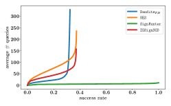
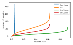
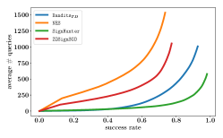
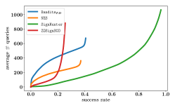
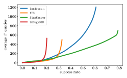
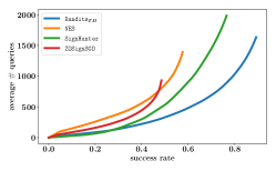
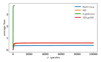
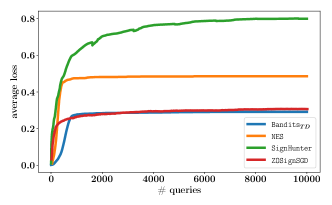
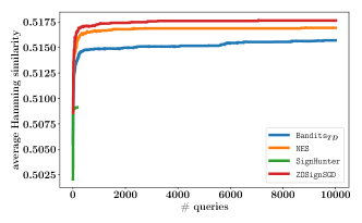
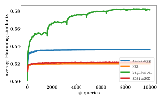
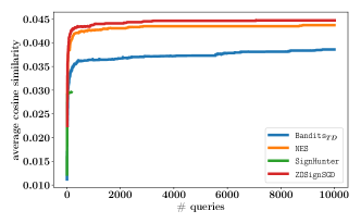
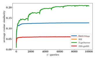
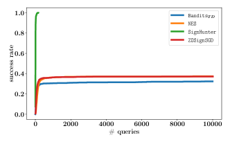
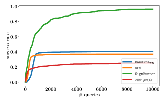
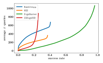
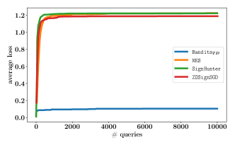
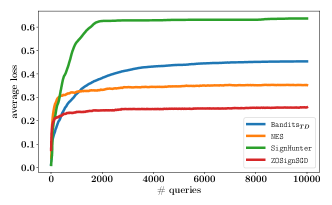
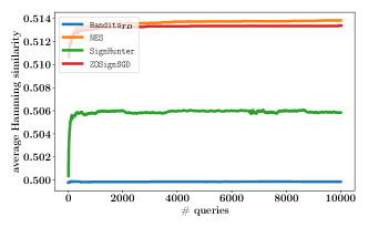
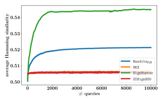
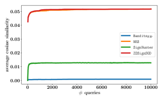
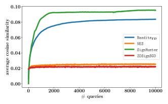
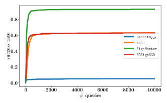
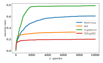
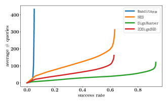
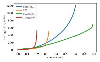
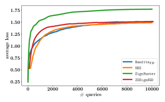
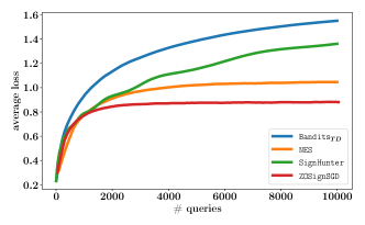
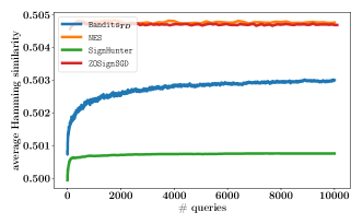
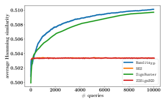
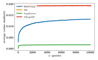
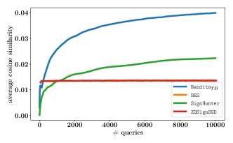
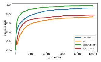
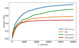
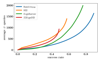
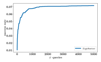
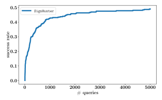
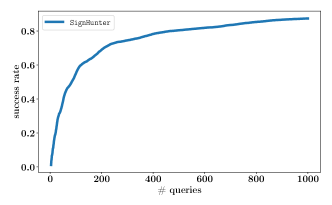
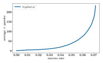
Figure 2 shows the trade-off between the success (evasion) rate and the mean number of queries (of the successful attacks) needed to generate an adversarial example for the MNIST, CIFAR10, and IMAGENET classifiers in the $\ell_{\infty}$ and $\ell_{2}$ perturbation constraints. In other words, these figures indicate the average number of queries required for a desired success rate. Tabulated summary of these plots can be found in Appendix E, namely Tables 6, 7, and 8. Furthermore, we plot the classifier loss and the gradient estimation quality (in terms of Hamming distance and Cosine similarity) averaged over all the images as a function of the number of queries used in Figures 10, 11, and 12 of Appendix E. Based on the results, we observe the following:

For any given success rate, SignHunter dominates the previous state of the art approaches in all settings except the IMAGENET $\ell_{2}$ setup, where Bandits_TD shows a better query efficiency when the desired success rate is greater than or equal $\sim 0.35$. Our approach is remarkably efficient in the $\ell_{\infty}$ setup (e.g., achieving a $\bf 100\%$ evasion using—on average—just $\bf 12$ queries per image against the MNIST classifier!). Its performance degrades—yet, still outperforms the rest, most of the time—in the $\ell_{2}$ setup. This is expected, since SignHunter perturbs all the coordinates with the same magnitude and the $\ell_{2}$ perturbation bound $\epsilon_{2}$ for all the datasets in our experiments is set such that $\epsilon_{2}/\sqrt{n}\ll\epsilon_{\infty}$ as shown in Table 1 of Appendix D. Take the case of MNIST ($n=28\times 28$), where $\epsilon_{\infty}=0.3$ and $\epsilon_{2}=3$. For SignHunter, the $\ell_{2}$ setup is equivalent to an $\ell_{\infty}$ perturbation bound of $3/28\approx 0.1$. The employed $\ell_{2}$ perturbation bounds give the state of the art—continuous optimization based—approaches more perturbation options. For instance, it is possible for NES to perturb just one pixel in an MNIST image by a magnitude of $3$; two pixels by a magnitude of $2.1$ each; ten pixels by a magnitude of $0.9$ each, etc. On the other hand, the binary optimization view of SignHunter limits it to always perturb all $28\times 28$ pixels by a magnitude of $0.1$. Despite its less degrees of freedom, SignHunter maintains its effectiveness in the $\ell_{2}$ setup. The plots can be viewed as a sensitivity assessment of SignHunter as $\epsilon$ gets smaller for each dataset. Moreover, the performance of SignHunter is in line with Theorem 3 when compared with the performance of FGSM (the noisy FGSM at $k=100\%$ in Figures 1 and 2 of Appendix A) in both $\ell_{\infty}$ and $\ell_{2}$ setups for MNIST and CIFAR10—for IMAGENET, $2n=536,406$ is beyond our query budget of $10,000$ queries. For example, FGSM has a failure rate of $0.32$ for CIFAR10 $\ell_{2}$ (Appendix A, Figure 2 (b)), while SignHunter achieves a failure rate of $0.21$ with $692.39<2n=2\times 3\times 32\times 32=6144$ queries (Appendix E, Table 7).

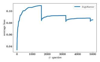
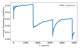
Incorporating SignHunter in an iterative framework of perturbing the data point $\bm{x}$ till the query budget is exhausted (Lines 10 to 14 in Algorithm 2) supports the observation in white-box settings that iterative FGSM—or Projected Gradient Descent (PGD)—is stronger than FGSM (Madry et al., 2017; Al-Dujaili et al., 2018). This is evident by the upticks in SignHunter’s performance on the MNIST $\ell_{2}$ case (Figure 10 of Appendix E: classifier’s loss, Cosine and Hamming similarity plots), which happens after every iteration (after every other $2\times 28\times 28$ queries). Plots of the Hamming similarity capture the quality of the gradient sign estimation in terms of Eq. 2, while plots of the average Cosine similarity capture it in terms of Eq. 12. Both SignHunter and Bandits_TD consistently optimize both objectives. In general, SignHunter enjoys a faster convergence especially on the Hamming metric as it is estimating the signs compared to Bandits_TD’s full gradient estimation. This is highlighted in the IMAGENET $\ell_{2}$ setup. Note that once an attack is successful, the gradient sign estimation at that point is used for the rest of the plot. This explains why, in the $\ell_{\infty}$ settings, SignHunter’s plot does not improve compared to its $\ell_{2}$ counterpart, as most of the attacks are successful in the very first few queries made to the loss oracle.

Overall, SignHunter is $3.8\times$ less failure-prone than the state-of-the-art approaches combined, and spends over all the images (successful and unsuccessful attacks) $2.5\times$ less queries. The number of queries spent is computed based on Tables 6, 7, and 8 of Appendix E as
 0.75cm  (1 - fail_rate) * avg_#_queries + fail_rate * 10,000.

6 Attack Effectiveness Under Defenses

Table 1: Top-3 attacks on the MNIST black-box challenge. Adapted from the challenge’s website—as of Feb 22, 2019.

Black-Box Attack	Model Accuracy
SignHunter (Algorithm 2)	$\bf 91.47\%$
(Xiao et al., 2018)	$92.76\%$
PGD against three independently and adversarially trained copies of the network	$93.54\%$

Table 2: Top-3 attacks for the CIFAR10 black-box challenge. Adapted from the challenge’s website—as of Feb 22, 2019.

Black-Box Attack	Model Accuracy
SignHunter (Algorithm 2)	$\bf 47.16\%$
PGD on the cross-entropy loss for the adversarially trained public network	$63.39\%$
PGD on the CW loss for the adversarially trained public network	$64.38\%$

Table 3: Top 1 Error percentage. The numbers between brackets are computed on 10,000 images from the validation set. The rest are from (Tramèr et al., 2017, Table 4).

Model	clean	Max. Black-box	SignHunter
			after 20 queries	after 1000 queries
v3${}_{\text{adv-ens4}}$	24.2 (26.73)	33.4	(40.61)	(90.75)

To complement our results in Section 5, we evaluated SignHunter against adversarial training, an effective way to improve the robustness of DNNs (Madry et al., 2017). In particular, we attacked the secret models used in public challenges for MNIST and CIFAR10. There was no corresponding challenge for IMAGENET. Instead, we used ensemble adversarial training, a method that argues security against black-box attacks based on transferability/substitute models (Tramèr et al., 2017). The same metrics used in Section 5 are recorded for the experiments here in Appendix F.

Public MNIST Black-Box Attack Challenge.

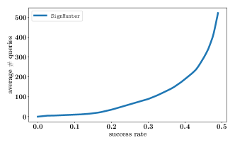
In line with the challenge setup, $10,000$ test images were used with an $\ell_{\infty}$ perturbation bound of $\epsilon=0.3$. Although the secret model is released, we treated it as a black box similar to our experiments in Section 5. No maximum query budget was specified, so we set it to $5,000$ queries. This is similar to the number of iterations given to a PGD attack in the white-box setup of the challenge: 100-steps with 50 random restarts. As shown in Table 1, SignHunter’s attacks resulted in the lowest model accuracy of $\bf 91.47\%$, outperforming all other state-of-the-art black-box attack strategies submitted to the challenge with an average number of queries of $\bf 233$ per successful attack. We would like to note that the attacks submitted to the challenge are based on transferability and do not query the model of interest. On the other hand, the most powerful white-box attack by Zheng et al. (2018)—as of Feb 22, 2019—resulted in a model accuracy of $88.56\%$–not shown in the table. Further, a PGD attack with $5000$ iterations/back-propagations ($100$ steps and $50$ random restarts) achieves $89.71\%$ in contrast to SignHunter’s $91.47\%$ with just $5000$ forward-propagations.

Public CIFAR10 Black-Box Attack Challenge.

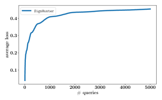
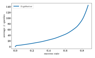
In line with the challenge setup, $10,000$ test images were used with an $\ell_{\infty}$ perturbation bound of $\epsilon=8$. Although the secret model is released, we treated it as a black box similar to our experiments in Section 5. Similar to the MNIST challenge, the query budget is $5,000$ queries. From Table 2, SignHunter’s attacks resulted in the lowest model accuracy of $\bf 47.16\%$, outperforming all other state-of-the-art black-box attack strategies submitted to the challenge with an average number of queries of $\bf 569$ per successful attack. We would like to note that the attacks submitted to the challenge are based on transferability and do not query the model of interest. On the other hand, the most powerful white-box attack by Zheng et al. (2018), —as of Feb 22, 2019—resulted in a model accuracy of $44.71\%$–not shown in the table. Further, a PGD attack with $200$ iterations/back-propagations ($20$ steps and $10$ restarts) achieves $45.71\%$ in contrast to SignHunter’s $47.16\%$ with $5000$ forward-propagations.

Ensemble Adversarial Training on IMAGENET.

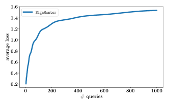
In line with (Tramèr et al., 2017), we set $\epsilon=0.0625$ and report the model’s misclassification over 10,000 random images from IMAGENET’s validation set. We attack the v3${}_{\text{adv-ens4}}$ model. As shown in Table 3, after $20$ queries, SignHunter achieves a top-1 error of $40.61\%$ greater than the $33.4\%$ rate of a series of black-box attacks (including PGD with $20$ iterations) transferred from a substitute model. With $1000$ queries, SignHunter breaks the model’s robustness with a top-1 error of $90.75\%$!

(a) $\ell_{\infty}$ perturbation	(b) $\ell_{2}$ perturbation

Figure 3: Illustration of adversarial examples crafted by SignHunter in comparison to attacks that are based on the continuous optimization in both (a) $\ell_{\infty}$ and (b) $\ell_{2}$ settings. If SignHunter is given a query budget $>2n$, which is the case here, the crafted adversarial examples are not necessary at the perturbation vertices, e.g., the red ball 2. We can modify SignHunter to strictly look up perturbation vertices. This could be done by doubling the step size from $\epsilon_{\infty}$ to $2\epsilon_{\infty}$ and we leave this for future work as outlined in Section 7.

7 Open Questions

(a) $n=10$	(b) $n=100$	(c) $n=1,000$	(d) $n=100,000$

Figure 4: SignHunter for continuous optimization. In this basic experiment, we run NES, ZO-SignSGD and SignHunter to minimize a function $f:\mathbb{R}^{n}\to\mathbb{R}$ of the form $||\bm{x}-\bm{x}^{*}||^{2}_{2}$ for $n\in\{10,100,1000,100000\}$. The solid line represents the loss averaged over 30 independent trials with random $\bm{x}^{*}\sim\mathcal{U}([0,1]^{n})$ and the shaded region indicates the standard deviation of results over random trials. We used a fixed step size of $0.01$ in line with (Liu et al., 2019) and a finite difference perturbation of $0.001$. The starting point $\bm{x}^{(0)}$ for all the algorithms was set to be the all-one vector $\mathbf{1}_{n}$.

There are many interesting questions left open by our research:

Priors.

Current version of SignHunter does not exploit any data- or time-dependent priors. With these priors, algorithms such as Bandits_TD operate on a search space of dimensionality $\sim 36\times$ less than that of SignHunter for IMAGENET. In domain-specific examples such as images, can Binary Partition Trees (BPT) (Al-Dujaili et al., 2015) be incorporated in SignHunter to have a data-dependent grouping of gradient coordinates instead of the current equal-size grouping?

Adversarial Training.

Compared to other attacks that are based on transferability and generative adversarial networks, our approach showed more effectiveness towards (ensemble) adversarial training. Standard adversarial training relies on attacks that employ iterative continuous optimization methods such as PGD in contrast to our attack which stems from a binary optimization view. What are the implications?

Other Domains.

Much of the work done to understand and counter adversarail examples has occurred in the image classification domain. The binary view of our approach lends itself naturally to other domains where binary features are used (e.g., malware detection (Al-Dujaili et al., 2018; Demetrio et al., 2019)). How effective our approach is on these domains?

Perturbation Vertices.

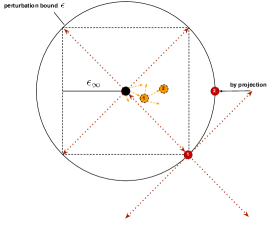
Using its first $O(n)$ queries, SignHunter probes $O(n)$ extreme points of the perturbation region as potential adversarial examples, while iterative continuous optimization such as NES probes points in the Gaussian sphere around the current point as shown in Figure 3. Does looking up extreme points (vertices) of the perturbation region suffice to craft adversarial examples? If that is the case, how to efficiently search through them? SignHunter searches through $2n$ vertices out of $2^{n}$ and it could find adversarial examples among a tiny fraction of these vertices. Recall, in the MNIST $\ell_{\infty}$ setup in Section 5, it was enough to look up just $\sim 12$ out of $2^{784}$ vertices for each image achieving a $100\%$ evasion over $1,000$ images. Note that after $2n$ queries, SignHunter may not visit other vertices as they will be $2\epsilon_{\infty}$ away as shown in Figure 3. We ignored this effect in our experiments. Will SignHunter be more effective if the probes are made strictly at the perturbation vertices? This question shows up clearly in the public MNIST challenge where the loss value at the potential adversarial examples dips after every $\sim 2n$ queries (see top left plot of Figure 13 in Appendix!F). We conjecture the reason is that these potential adversarial examples are not extreme points as illustrated in Figure 3: they are like the red ball 2 rather than the red ball 1.

SignHunter for Black-Box Continuous Optimization.

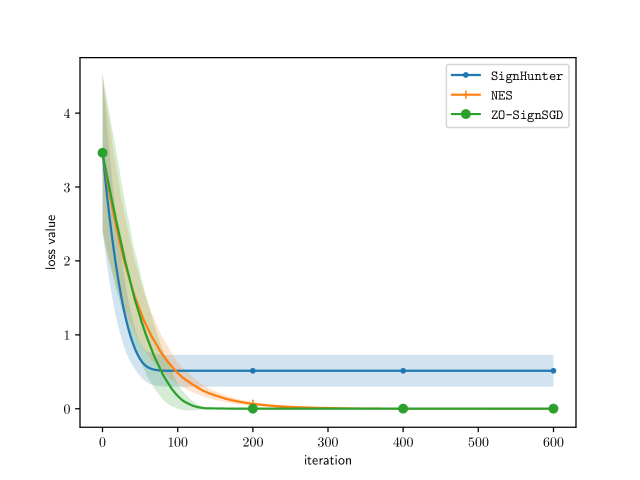
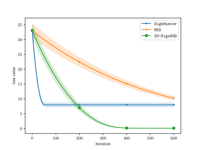
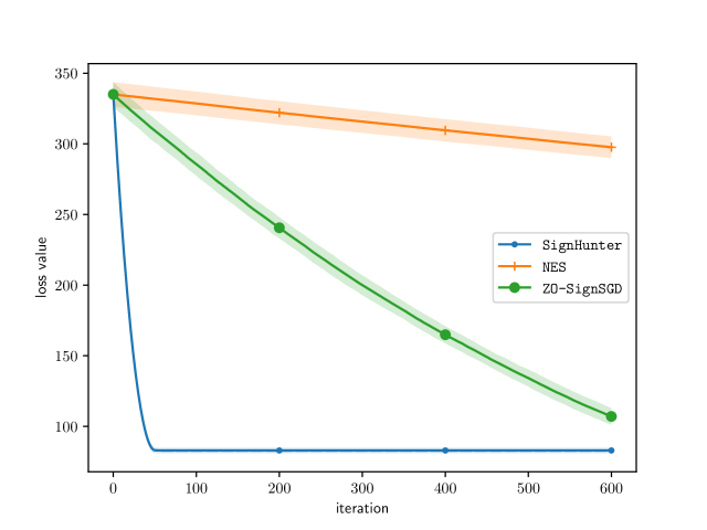
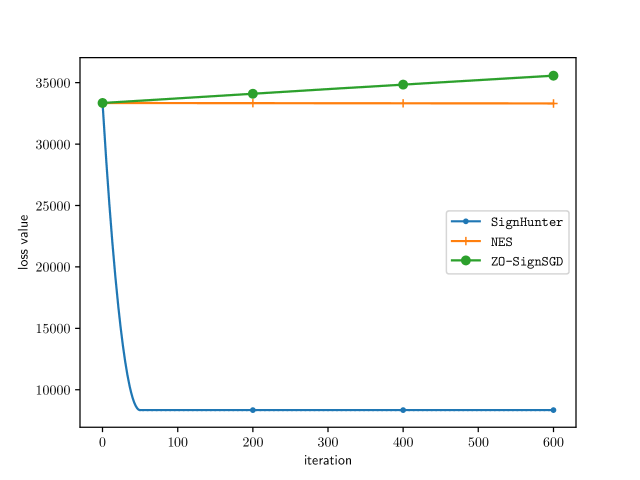
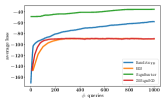
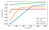
In (Salimans et al., 2017; Chrabaszcz et al., 2018), it was shown that a class of black-box continuous optimization algorithms (NES as well as a very basic canonical ES algorithm) rival the performance of standard reinforcement learning techniques. On the other hand, SignHunter is tailored towards recovering the gradient sign bits and creating adversarial examples similar to FGSM using the best gradient sign estimation obtained so far. Can we incorporate SignHunter in an iterative framework for continuous optimization? Figure 4 shows a small, preliminary experiment comparing NES and ZO-SignSGD to a simple iterative framework employing SignHunter. In the regime of high dimension/few iterations, SignHunter can be remarkably faster. However, with more iterations, the algorithm fails to improve further and starts to oscillate. The reason is that SignHunter always provides $\pm 1$ updates (non-standard sign convention) compared to the other algorithms whose updates can be zero. Can we get the best of both worlds?

8 Conclusion

Assuming a black-box threat model, we studied the problem of generating adversarial examples for neural nets and proposed the gradient sign estimation problem as the core challenge in crafting these examples. We formulate the problem as a binary black-box optimization one: minimizing the Hamming distance to the gradient sign or, equivalently, maximizing the directional derivative. Approximated by the finite difference of the loss value queries, we examine three properties of the directional derivative of the model’s loss in the direction of $\{\pm 1\}^{n}$ vectors. The separability property helped us devise SignHunter, a divide-and-conquer algorithm that is guaranteed to perform at least as well as FGSM after $O(n)$ queries. In practice, SignHunter needs a fraction of this number of queries to craft adversarial examples. To verify its effectiveness on real-world datasets, SignHunter was evaluated on neural network models for the MNIST, CIFAR10, and IMAGENET datasets. SignHunter yields black-box attacks that are $2.5\times$ more query efficient and $3.8\times$ less failure-prone than the state of the art attacks combined. Moreover, SignHunter achieves the highest evasion rate on two public black-box attack challenges. We also show that models that are robust against substitute-model attacks are vulnerable to our attack.

Appendix A. Noisy FGSM

This section shows the performance of the noisy FGSM on standard models (described in Section 5 of the main paper) on the MNIST, CIFAR10 and IMAGENET datasets. In Figure 5, we consider the $\ell_{\infty}$ threat perturbation constraint. Figure 6 reports the performance for the $\l 2$ setup. Similar to (Ilyas et al., 2019), for each $k$ in the experiment, the top $k$ percent of the signs of the coordinates—chosen either randomly (random-k) or by the corresponding magnitude $|\partial L(\bm{x},y)/\partial x_{i}|$ (top-k)—are set correctly, and the rest are set to $-1$ or $+1$ at random. The misclassification rate shown considers only images that were correctly classified (with no adversarial perturbation). In accordance with the models’ accuracy, there were $987$, $962$, and $792$ such images for MNIST, CIFAR10, and IMAGENET out of the sampled $1000$ images, respectively. These figures also serve as a validation for Theorem 3 when compared to SignHunter’s performance shown in Appendix C.

(a)	(b)	(c)

Figure 5: Misclassification rate of three neural nets (for (a) MNIST, (b) CIFAR10, and (c) IMAGENET, respectively) on the noisy FGSM’s adversarial examples as a function of correctly estimated coordinates of $\operatorname{sign}(\nabla_{\bm{x}}f(\bm{x},y))$ on random $1000$ images from the corresponding evaluation dataset, with the maximum allowed $\ell_{\infty}$ perturbation $\epsilon$ being set to $0.3$, $12$, and $0.05$, respectively. Across all the models, estimating the sign of the top $30\%$ gradient coordinates (in terms of their magnitudes) is enough to achieve a misclassification rate of $\sim 70\%$. Note that Plot (c) is similar to (Ilyas et al., 2019)’s Figure 1, but it is produced with TensorFlow rather than PyTorch.

(a)	(b)	(c)

Figure 6: Misclassification rate of three neural nets (for (a) MNIST, (b) CIFAR10, and (c) IMAGENET, respectively) on the noisy FGSM’s adversarial examples as a function of correctly estimated coordinates of $\operatorname{sign}(\nabla_{\bm{x}}f(\bm{x},y))$ on random $1000$ images from the corresponding evaluation dataset, with the maximum allowed $\ell_{2}$ perturbation $\epsilon$ being set to $3$, $127$, and $5$, respectively. Compared to Figure 5, the performance on MNIST and CIFAR10 drops significantly.

Appendix B. A Framework for Estimating Sign of the Gradient from Loss Oracles

Our interest in this section is to estimate the gradient sign bits of the loss function $L$ of the model under attack at an input/label pair ($\bm{x},y$) from a limited number of loss value queries $L(\bm{x}^{\prime},y)$. To this end, we examine the basic concept of directional derivatives that has been employed in recent black-box adversarial attacks. Particularly, we present three approaches to estimate the gradient sign bits based on three properties of the directional derivative $D_{\bm{q}}L(\bm{x},y)$ of the loss in the direction of a sign vector $\bm{q}\in\mathcal{H}$.

Approach 1: Divide & Conquer

Covered in the main article.

Approach 2: Loss Oracle as a Noisy Hamming Oracle

The directional derivative of the loss function $L$ at $(\bm{x},y)$ in the direction of a binary code $\bm{q}$ can be written as

$$D_{\bm{q}}L(\bm{x},y) = \bm{q}^{T}\bm{g}^{*}$$ (5)

$$= \sum_{i\in\mathcal{I}^{+}_{\bm{q}}}|g^{*}_{i}|-\sum_{i\in\mathcal{I}^{-}_{\bm{q}}}|g^{*}_{i}|$$

$$= |\mathcal{I}^{+}_{q}|\bar{g}_{\mathcal{I}^{+}_{\bm{q}}}-|\mathcal{I}^{-}_{q}|\bar{g}_{\mathcal{I}^{-}_{\bm{q}}}\;,$$

where $\mathcal{I}^{+}_{\bm{q}}\equiv\{i\mid i\in[n]\;,\;q^{*}_{i}=q_{i}\}$, $\mathcal{I}^{-}_{\bm{q}}\equiv[n]\setminus\mathcal{I}^{+}_{\bm{q}}$. Note that $|\mathcal{I}^{+}_{q}|+|\mathcal{I}^{-}_{q}|=n$. The quantities $\bar{g}_{\mathcal{I}^{+}_{\bm{q}}}$ and $\bar{g}_{\mathcal{I}^{-}_{\bm{q}}}$ are the means of $\{|g_{i}|\}_{i\in\mathcal{I}^{+}_{\bm{q}}}$ and $\{|g_{i}|\}_{i\in\mathcal{I}^{-}_{\bm{q}}}$, respectively. Observe that $|\mathcal{I}^{-}_{\bm{q}}|=||\bm{q}-\bm{q}^{*}||_{H}:$ the Hamming distance between $\bm{q}$ and the gradient sign $\bm{q}^{*}$. In other words, the directional derivative $D_{\bm{q}}L(\bm{x},y)$ has the following property.

Property 2.

The directional derivative $D_{\bm{q}}L(\bm{x},y)$ of the loss function $L$ at an input/label pair $(\bm{x},y)$ in the direction of a binary code $\bm{q}$ can be written as an affine transformation of the Hamming distance between $\bm{q}$ and $\bm{q}^{*}$. Formally, we have

$$D_{\bm{q}}L(\bm{x},y)=n\bar{g}_{\mathcal{I}^{+}_{\bm{q}}}-(\bar{g}_{\mathcal{I}^{-}_{\bm{q}}}+\bar{g}_{\mathcal{I}^{+}_{\bm{q}}})||\bm{q}-\bm{q}^{*}||_{H}$$ (6)

If we can recover the Hamming distance from the directional derivative based on Eq. 6, efficient Hamming search strategies—e.g., (Maurer, 2009)—can then be used to recover the gradient sign bits $\bm{q}^{*}$ with a query complexity $\Omega(n/\log_{2}(n+1))$ as stated in Theorem 1. However, not all terms of Eq. 6 is known to us. While $n$ is the number of data features (known a priori) and $D_{\bm{q}}L(\bm{x},y)$ is available through a finite difference oracle, $\bar{g}_{\mathcal{I}^{+}_{\bm{q}}}$ and $\bar{g}_{\mathcal{I}^{-}_{\bm{q}}}$ are not known. Here, we propose to approximate these values by their Monte Carlo estimates: averages of the magnitude of sampled gradient components. Our assumption is that the magnitudes of gradient coordinates are not very different from each other, and hence a Monte Carlo estimate is good enough (with small variance). Our experiments on MNIST, CIFAR10, and IMAGENET confirm the same—see Figure 18 in Appendix G.

To use the $i$th gradient component $g^{*}_{i}$ as a sample for our estimation, one can construct two binary codes $\bm{u}$ and $\bm{v}$ such that only their $i$th bit is different, i.e., $||\bm{u}-\bm{v}||_{H}=1$. Thus, we have

$$|g^{*}_{i}| = \frac{|D_{\bm{u}}L(\bm{x},y)-D_{\bm{v}}L(\bm{x},y)|}{2}$$ (7)

$$q^{*}_{i}=\operatorname{sign}(g^{*}_{i}) = \begin{cases}u_{i}&\text{if }D_{\bm{u}}L(\bm{x},y)>D_{\bm{v}}L(\bm{x},y)\;,\\ v_{i}&\text{otherwise}\;.\end{cases}$$ (8)

Let $\mathcal{D}$ be the set of indices of gradient components we have recovered—magnitude and sign—so far through Eq. 7 and Eq. 8. Then,

$$\bar{g}_{\mathcal{I}^{+}_{\bm{q}}}\approx\frac{1}{|\mathcal{D}^{+}_{\bm{q}}|}\sum_{d\in\mathcal{D}^{+}_{\bm{q}}}|g^{*}_{d}|\;,$$ (9)

$$\bar{g}_{\mathcal{I}^{-}_{\bm{q}}}\approx\frac{1}{|\mathcal{D}^{-}_{\bm{q}}|}\sum_{d\in\mathcal{D}^{-}_{\bm{q}}}|g^{*}_{d}|\;,$$ (10)

where $\mathcal{D}^{+}_{\bm{q}}\equiv\{d\mid d\in\mathcal{D}\;,\;q^{*}_{d}=q_{i}\}$ and $\mathcal{D}^{-}_{\bm{q}}\equiv\mathcal{D}\setminus\mathcal{D}^{+}_{\bm{q}}$. As a result, the Hamming distance between $\bm{q}$ and the gradient sign $\bm{q}^{*}$ can be approximated with the following quantity, which we refer to as the noisy Hamming oracle $\hat{\mathcal{O}}$.

$$||\bm{q}-\bm{q}^{*}||_{H}\;\approx\;\frac{\frac{n}{|\mathcal{D}^{+}_{\bm{q}}|}\sum_{d\in\mathcal{D}^{+}_{\bm{q}}}|g^{*}_{d}|-D_{\bm{q}}L(\bm{x},y)}{\frac{1}{|\mathcal{D}^{+}_{\bm{q}}|}\sum_{d\in\mathcal{D}^{+}_{\bm{q}}}|g^{*}_{d}|+\frac{1}{|\mathcal{D}^{-}_{\bm{q}}|}\sum_{d\in\mathcal{D}^{-}_{\bm{q}}}|g^{*}_{d}|}$$ (11)

(a) $n=5$	(b) $n=10$

Figure 7: The error distribution of the noisy Hamming oracle $\hat{\mathcal{O}}$ (right side of Eq. 11) compared to the noiseless counterpart $\mathcal{O}$ (left side of Eq. 11) as a function of the number of unique values (magnitudes) of the gradient coordinates $m$. Here, $L(\bm{x},y)$ has the form $\mathbf{c}^{T}\bm{x}$. That is, $m=|\texttt{uniq}(|\mathbf{c}|)|\leq n$ with $n\in\{5,10\}$ being the input length. With $m=1$, the estimation is exact ($\hat{\mathcal{O}}=\mathcal{O}$) for all the binary code queries $\bm{q}$—32 codes for $n=5$, 1028 codes for $n=10$. The error seems to be bounded by $\lceil\frac{n}{2}\rceil$. For a given $m$, $c_{i}$—the $i^{th}$ coordinate of $\mathbf{c}$—is randomly assigned a value from the $m$ evenly spaced numbers in the range $[0.1,m/n]$. We set the size of the sampled gradient coordinates set $|\mathcal{D}|$ to $\lfloor n/4\rfloor$.

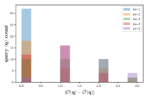
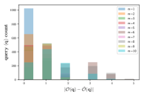
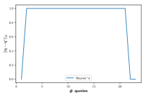
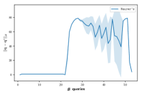
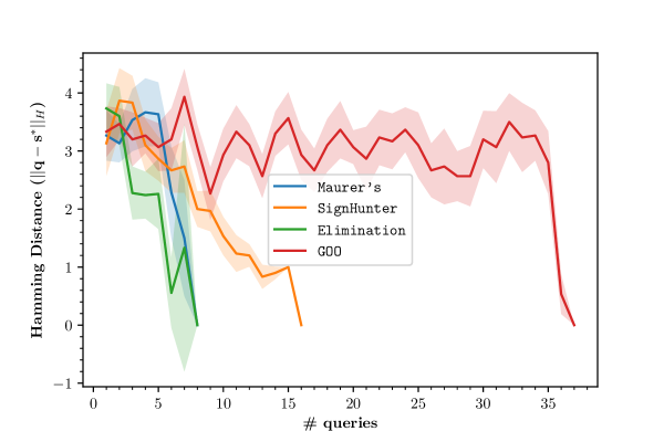
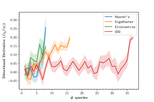
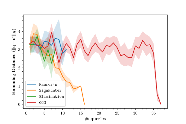
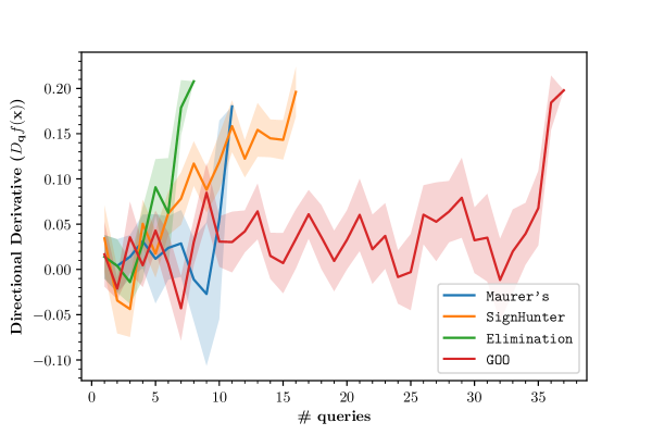
We empirically evaluated the quality of $\hat{\mathcal{O}}$’s responses on a toy problem where we controlled the magnitude spread/concentration of the gradient coordinates with $m$ being the number of unique values (magnitudes) of the gradient coordinates. As detailed in Figure 7, the error can reach $\lceil n/2\rceil$. This a big mismatch, especially if we recall the Hamming distance’s range is $[0,n]$. The negative impact of this on the Hamming search strategy by Maurer (2009) was verified empirically in Figure 8. We considered the simplest case where Maurer’s was given access to the noisy Hamming oracle $\hat{\mathcal{O}}$ in a setup similar to the one outlined in Figure 7, with $n=80$, $|\mathcal{D}|=n/4=20$, $m\in\{1,2\}$, and the hidden code $\bm{q}^{*}=[+1,\ldots,+1]$. To account for the randomness in constructing $\mathcal{D}$, we ran $30$ independent runs and plot the average Hamming distance (with confidence bounds) over Maurer’s queries. In Figure 8 (a), $m=1$ which corresponds to exact estimation $\hat{\mathcal{O}}=\mathcal{O}$, Maurer’s spends $21$ queries to construct $\mathcal{D}$ and terminates one query afterwards with the true binary code $\bm{q}^{*}$, achieving a query ratio of 21/80. On the other hand, when we set $m=2$ in Figure 8 (b); Maurer’s returns a 4-Hamming-distance away solution from the true binary code $\bm{q}^{*}$ after $51$ queries. This is not bad for an $80$-bit long code. However, this is in a tightly controlled setup where the gradient magnitudes are just one of two values. To be studied further is the bias/variance decomposition of the returned solution and the corresponding query ratio. We leave this investigation for future work.

(a) $m=1$	(b) $m=2$

Figure 8: Performance of Maurer’s on the noisy Hamming oracle $\hat{\mathcal{O}}$. The setup is similar to that of Figure 7, with $n=80$ and $m\in\{1,2\}$.

Approach 3: Optimism in the Face of Uncertainty

In the previous approach, we considered the approximated Hamming distance (Eq. 11) as a surrogate for the formal optimization objective (Eq. 3 in the main paper) of the gradient sign estimation problem. We found that current Hamming search strategies are not robust to approximation error. In this approach, we consider maximizing the directional derivative (Eq. 4 in the main paper)

$$\max_{\bm{q}\in\mathcal{H}}D_{\bm{q}}L(\bm{x},y)\;,$$ (12)

as our formal objective of the gradient sign estimation problem. Formally, we treat the problem as a binary black-box optimization over the $2^{n}$ hypercube vertices, which correspond to all possible sign vectors. This is significantly worse than $O(n)$ of the continuous optimization view. Nevertheless, the rationale here is that we do not need to solve Eq. 12 to optimality (recall the effectiveness of noisy FGSM in Appendix A); we rather need a fast convergence to a suboptimal but adversarially helpful sign vector $\bm{q}$. In addition, the continuous optimization view often employs an iterative scheme of $T$ steps within the perturbation ball $B_{p}(\bm{x},\epsilon)$, calling the gradient estimation routine in every step leading to a search complexity of $nT$. In our setup, we use the best obtained solution for Eq. 12 so far in a similar fashion to the noisy FGSM. In other words, our gradient sign estimation routine runs at the top level of our adversarial example generation procedure instead of calling it as a subroutine. In this and the next approach, we address the following question: how do we solve Eq. 12?

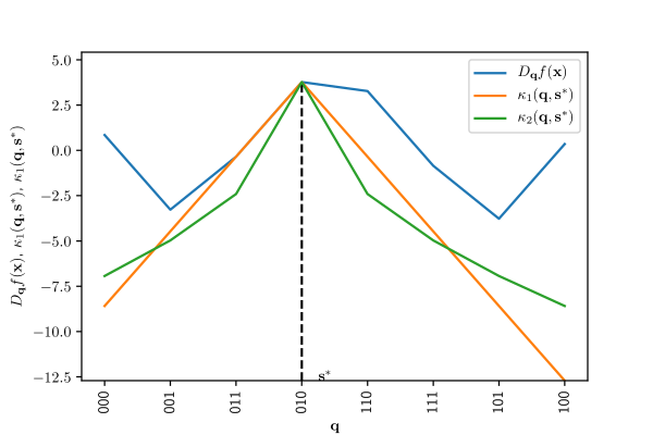
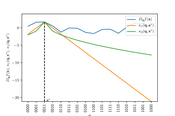
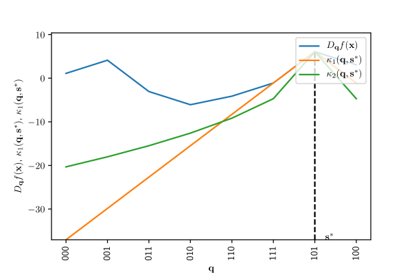
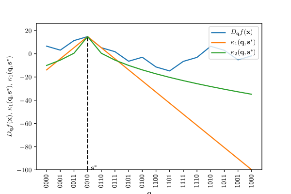
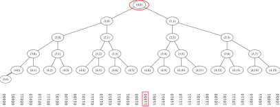
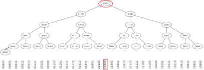
Optimistic methods, i.e., methods that implement the optimism in the face of uncertainty principle have demonstrated a theoretical as well as empirical success when applied to black-box optimization problems (Munos, 2011; Al-Dujaili & Suresh, 2017, 2018). Such a principle finds its foundations in the machine learning field addressing the exploration vs. exploitation dilemma, known as the multi-armed bandit problem. Within the context of function optimization, optimistic approaches formulate the complex problem of optimizing an arbitrary black-box function $g$ (e.g., Eq. 12) over the search space ($\mathcal{H}$ in this paper) as a hierarchy of simple bandit problems (Kocsis & Szepesvári, 2006) in the form of space-partitioning tree search $\mathcal{T}$. At step $t$, the algorithm optimistically expands a leaf node (partitions the corresponding subspace) from the set of leaf nodes $\mathcal{L}_{t}$ that may contain the global optimum. The $i^{th}$ node at depth $h$, denoted by $(h,i)$, corresponds to the subspace/cell $\mathcal{H}_{h,i}$ such that $\mathcal{H}=\cup_{0\leq i<K^{h}}\mathcal{H}_{h,i}$. To each node $(h,i)$, a representative point $\bm{q}_{h,i}\in\mathcal{H}_{h,i}$ is assigned, and the value of the node $(h,i)$ is set to $g(\bm{q}_{h,i})$. See Figure 11 for an example of a space-partitioning tree $\mathcal{T}$ of $\mathcal{H}$, which will be used in our second approach to estimate the gradient sign vector.

Under some assumptions on the optimization objective and the hierarchical partitioning $\mathcal{T}$ of the search space, optimistic methods enjoy a finite-time bound on their regret $R_{t}$ defined as

$$R_{t}=g(\bm{q}^{*})-g(\bm{q}(t))\;,$$ (13)

where $\bm{q}(t)$ is the best found solution by the optimistic method after $t$ steps. The challenge is how to align the search space such that these assumptions hold. In the following, we show that these assumptions can be satisfied for our optimization objective (Eq. 12). In particular, when $g(\bm{q})$ is the directional derivative function $D_{\bm{q}}L(\bm{x},y)$, and $\mathcal{H}$’s vertices are aligned on a 1-dimensional line according to the Gray code ordering, then we can construct an optimistic algorithm with a finite-time bound on its regret. To demonstrate this, we adopt the Simultaneous Optimistic Optimization framework by Munos (2011) and the assumptions therein.

	$n=3$	$n=4$
	(a)	(b)
	(c)	(d)

Figure 9: The directional derivative $D_{\bm{q}}f(\bm{x})$ of some function $f$ at a point $\bm{x}$ in the direction of a binary vector $\bm{q}\in\mathcal{H}\equiv\{-1,+1\}^{n}$ is locally smooth around the gradient sign vector, $\bm{q}^{*}=\operatorname{sign}(\nabla_{\bm{x}}f(\bm{x}))\in\mathcal{H}$, when $\mathcal{H}$ is ordered over one coordinate as a sequence of Gray codes. The plots show the local smoothness property—with two semi-metrics $\kappa_{1}(\cdot,\cdot)$ and $\kappa_{2}(\cdot,\cdot)$—of the directional derivative of functions $f$ of the form $\mathbf{c}^{T}\bm{x}$ and $\bm{x}^{T}Q\bm{x}$ for $n\in\{3,4\}$, as tabulated in Plots (a), (c) and (b, d), respectively. The local smoothness is evident as $D_{\bm{q}^{*}}f(\bm{x})-D_{\bm{q}}f(\bm{x})\leq\kappa_{1}(\bm{q},\bm{q}^{*})$ and $D_{\bm{q}^{*}}f(\bm{x})-D_{\bm{q}}f(\bm{x})\leq\kappa_{2}(\bm{q},\bm{q}^{*})$ for all $\bm{q}\in\mathcal{H}$. The semi-metrics $\kappa_{1}(\bm{q},\bm{q}^{*})$ and $\kappa_{2}(\bm{q},\bm{q}^{*})$ have the form $K|\texttt{rank}_{Gray}(\bm{q})-\texttt{rank}_{Gray}(\bm{q}^{*})|^{\alpha}$, where $\texttt{rank}_{Gray}(\cdot)$ refers to the rank of an $n$-binary code in the Gray ordering of $n$-binary codes (e.g., $\texttt{rank}_{Gray}([-1,-1,+1,-1])=4$), $K>0$ , and $\alpha>0$. With this property at hand, we employ the optimism in the face of uncertainty principle in GOO to maximize $D_{\bm{q}}f(\bm{x})$ over $\mathcal{H}$. For legibility, we replaced $-1$ with $0$ when enumerating $\mathcal{H}$ on the x-axis.

For completeness, we reproduce (Munos, 2011)’s basic definitions and assumptions with respect to our notation. At the same time we show how the gradient sign estimation problem (Eq. 12) satisfies them based on the second property of the directional derivative as follows.

Definition 2 (Semi-metric).

We assume that $\kappa:\mathcal{H}\times\mathcal{H}\to\operatorname{\mathbb{R}}^{+}$ is such that for all $\bm{p},\bm{q}\in\mathcal{H}$, we have $\kappa(\bm{p},\bm{q})=\kappa(\bm{q},\bm{p})$ and $\kappa(\bm{p},\bm{q})=0$ if and only if $\bm{p}=\bm{q}$.

Definition 3 (Near-optimality dimension).

The near-optimal dimension is the smallest $d\geq 0$ such that there exists $C>0$ such that for any $\varepsilon>0$, the maximal number of disjoint $\kappa$-balls of radius $\upsilon\varepsilon$ and center in $\mathcal{H}_{\varepsilon}$ is less than $C\varepsilon^{-d}$.

Property 3 (Local smoothness of $D_{\bm{q}}L(\bm{x},y)$).

For any input/label pair $(\bm{x},y)$, there exists at least a global optimizer $\bm{q}^{*}\in\mathcal{H}$ of $D_{\bm{q}}L(\bm{x},y)$ (i.e., $D_{\bm{q}^{*}}L(\bm{x},y)=\sup_{\bm{q}\in\mathcal{H}}D_{\bm{q}}L(\bm{x},y)$) and for all $\bm{q}\in\mathcal{H}$,

$$D_{\bm{q}^{*}}L(\bm{x},y)-D_{\bm{q}}L(\bm{x},y)\leq\kappa(\bm{q},\bm{q}^{*})\;.$$

Refer to Figure 9 for a pictorial proof of Property 3.

Assumption 1 (Bounded diameters).

There exists a decreasing a decreasing sequence $\omega(h)>0$, such that for any depth $0\leq h<n$, for any cell $\mathcal{H}_{h,i}$ of depth $h$, we have $\sup_{\bm{q}\in\mathcal{H}_{h,i}}\kappa(\bm{q}_{h,i},\bm{q})\leq\omega(h)$.

To see how Assumption 1 is met, refer to Figure 11.

Assumption 2 (Well-shaped cells).

There exists $\upsilon>0$ such that for any depth $0\leq h<n$, any cell $\mathcal{H}_{h,i}$ contains a $\kappa$-ball of radius $\upsilon\omega(h)$ centered in $\bm{q}_{h,i}$.

To see how Assumption 2 is met, refer to Figure 11. With the above assumptions satisfied, we propose the Gray-code Optimistic Optimization (GOO), which is an instantiation of (Munos, 2011, Algorithm 2) tailored to our optimization problem (Eq. 12) over a 1-dimensional alignment of $\mathcal{H}$ using the Gray code ordering. The pseudocode is outlined in Algorithm 3. The following theorem bounds GOO’s regret.

Theorem 4.

Regret Convergence of GOO Let us write $h(t)$ the smallest integer $h$ such that

$$Ch_{max}(t)\sum_{l=0}^{h}\omega(l)^{-d}+1\geq t\;.$$ (14)

Then, with $g(\bm{q})=D_{\bm{q}}L(\bm{x},y)$, the regret of GOO (Algorithm 3) is bounded as

$$R_{t}\leq\omega(\min(h(t),h_{max}(t)+1))$$

Proof.

We have showed that our objective function (Eq. 12) and the hierarchical partitioning of $\mathcal{H}$ following the Gray code ordering confirm to Property 3 and Assumptions 1 and 2. The $+1$ term in Eq. 14 is to accommodate the evaluation of node $(n,0)$ before growing the space-partitioning tree $\mathcal{T}$—see Figure 11. The rest follows from the proof of (Munos, 2011, Theorem 2). ∎

Algorithm 3 Gray-code Optimistic Optimization (GOO)
Input:
$g:\mathcal{H}\to\operatorname{\mathbb{R}}$ : the black-box linear function to be maximized over the binary hypercube $\mathcal{H}\equiv\{-1,+1\}^{n}$ $h_{max}(t)$ : the maximum depth function which limits the tree to grow up to $h_{max}(t)+1$ after $t$ node expansions

  Initialization: Set $t=1$, $\mathcal{T}_{t}=\{(0,0)\}$ (root node). Align $\mathcal{H}$ over $\mathcal{T}_{t}$ using the Gray code ordering.

  while True do

   $v_{max}\leftarrow-\infty$

   for $h=0$ to $\min(depth(\mathcal{T}_{t}),h_{max}(t))$ do

     Among all leaves $(h,j)\in\mathcal{L}_{t}$ of depth $h$, select

$$(h,i)\in\operatorname*{arg\,max}_{(h,j)\in\mathcal{L}_{t}}g(\bm{q}_{h,i})$$

     if $g(\bm{q}_{h,i})\geq v_{max}$ then

      Expand this node: add to $\mathcal{T}_{t}$ the two children $(h+1,i_{k})_{1\leq k\leq 2}$

      $v_{max}\leftarrow g(\bm{q}_{h,i})$

      $t\leftarrow t+1$

      if query budget is exhaused then

        return the best found solution $\bm{q}(t)$.

      end if

     end if

   end for

  end while

Despite being theoretically-founded, GOO is slow in practice. This is expected since it is a global search technique that considers all the $2^{n}$ vertices of the $n$-dimensional hypercube $\mathcal{H}$. Recall that we are looking for adversarially helpful solution $\bm{q}$ that may not be necessarily optimal.

Empirical Evaluation of the Approaches on a Set of Toy Problems

We tested both GOO and SignHunter (along with Maurer’s and Elimination) on a set of toy problems and found that SignHunter performs significantly better than GOO, while Maurer’s and Elimination were sensitive to the approximation error—see Figure 10. We remind the reader that Maurer’s and Elimination are two search strategies for $\bm{q}^{*}$ using the Hamming oracle. After response $r^{(i)}$ to query $\bm{q}^{(i)}$, Elimination eliminates all binary codes $\bm{q}\in\mathcal{H}$ with $||\bm{q}-\bm{q}^{(i)}||_{H}\neq r^{(i)}$ in an iterative manner. Note that Elimination is a naive technique that is not scalable with $n$. For Maurer’s, we refer the reader to (Maurer, 2009).

	Hamming Distance Trace	Directional Derivative Trace
	(a)	(b)
	(c)	(d)

Figure 10: Noiseless vs. Noisy Hamming Oracle: The trace of the Hamming distance (first column, where the lower the trace the better) and directional derivative (second column, where the higher the trace the better) values of Elimination and Maurer’s queries, when given access to a noiseless/ideal (first row) and noisy Hamming oracles (second row)—through a directional derivative approximation as discussed in Approach 2—for a synthetic function $f$ of the form $\bm{x}^{T}Q\bm{x}$ with $n=7$. We expect the traces to go up and down as they explore the $2^{n}$ search space. The end of an algorithm’s trace represents the value of the Hamming distance (directional derivative) for the first column (for the second column) at the algorithm’s solution. For comparison, we also plot GOO and SignHunter’s traces. Note that the performance of GOO and SignHunter is the same in both noiseless and noisy cases as both algorithms operate directly on the directional derivative approximation rather than the noiseless/noisy Hamming oracle. In the case of noiseless Hamming oracle, both Elimination and Maurer’s finds the optimal vector $\bm{q}^{*}\in\mathcal{H}\equiv\{-1,+1\}^{7}$ with # queries $\leq 7$—their traces end at most at $8$ just to show that the algorithm’s solution achieves a zero Hamming distance as shown in Plot (a), which corresponds to the maximum directional derivative in Plot (b). With a noisy Hamming oracle, these algorithm break as shown in Plots (c) and (d): taking more than $n$ queries and returning sub-optimal solutions—e.g., Maurer’s returns on average a three-Hamming-distance solution. On the other hand, GOO and SignHunter achieve a zero Hamming distance in both cases at the expense of being less query efficient. While being theoretically-founded, GOO is slow as it employs a global search over the $2^{n}$ space. Despite SignHunter’s local search, it converges to the optimal solution after $2\times 7$ queries in accordance with Theorem 3. The solid curves indicate the corresponding averaged trace surrounded by a $95\%$-confidence bounds using $30$ independent runs. For convenience, we plot the symmetric bounds where in fact they should be asymmetric in Plots (a) and (c) as the Hamming distance’s range is $\mathbb{Z}^{+}_{0}.$

(a) $(h,i)$ view	(b) $\bm{q}_{h,i}$ view

Figure 11: Illustration of the proposed Gray-ordering based partitioning (fully expanded) tree $\mathcal{T}$ of the search space $\mathcal{H}=\{-1,+1\}^{n}$—with $n=5$—used in the Gray-code Optimistic Optimization (GOO). The plots are two different views of the same tree. Plot (a) displays the node name $(h,i)$, while Plot (b) shows its representative binary code $\bm{q}_{h,i}\in\mathcal{H}$. For brevity, we replaced $-1$s with $0$s. The red oval and rectangle highlights the tree’s root and its corresponding binary code, respectively. Consider the node $(2,1)$ whose representative code is $\bm{q}_{2,1}=[-1,+1,-1,+1,-1]$ and its corresponding subspace $\mathcal{H}_{2,1}=\{\bm{q}_{2,1},\bm{q}_{3,2},\bm{q}_{3,3},\bm{q}_{4,4},\bm{q}_{4,5},\bm{q}_{4,6},\bm{q}_{4,7}\}$. The same reasoning applies to the rest of the nodes. To maintain a valid binary partition tree, one can ignore the anomaly leaf node $(5,0)$, this corresponds to the code $\bm{q}_{5,0}=[-1,-1,-1,-1,-1]$, which in practice can be evaluated prior to building the tree. Let us consider the nodes at depth $h=2$, observe that for all $i\in\{0,1,2,3\}$ 1) $|\mathcal{H}_{2,i}|=7$ ; 2) $\bm{q}_{2,i}$ is centered around the other $6$ members of $\mathcal{H}_{2,i}$ in the Gray code ordering; and that 3) $\mathcal{H}_{2,i}$ constitutes a contiguous block of codes along the 1-dimensional alignment shown below the tree. Thus, it suffices to define a semi-metric based on the corresponding indices of the codes along this alignment. For a given depth $h$, the index of any code $\bm{q}\in\mathcal{H}_{h,i}$ is at most $\omega(h)=\sup_{j}|\mathcal{H}_{h+1,j}|$, which establishes Assumption 2. Assumption 3 follows naturally from the fact that nodes at a given depth $h$ partition the search space $\mathcal{H}$ equally (e.g., $|\mathcal{H}_{2,i}|=7$ for all $i$).

Appendix C. Proofs for Theorems in the Main Paper

Along with the proofs, we restate the theorems for completeness.

Theorem 2.

A hidden $n$-dimensional binary code $\bm{q}^{*}\in\mathcal{H}$ can be retrieved exactly with no more than $n$ queries to the noiseless Hamming oracle $\mathcal{O}$.

Proof.

The key element of this proof is that the Hamming distance between two $n$-dimensional binary codes $\bm{q},\bm{q}^{*}\in\mathcal{H}$ can be written as

$$r=||\bm{q}-\bm{q}^{*}||_{H}=\frac{1}{2}(n-\bm{q}^{T}\bm{q}^{*})\;.$$ (15)

Let $Q$ be an $n\times n$ matrix where the $i$th row is the $i$th query code $\bm{q}^{(i)}$. Likewise, let $r^{(i)}$ be the corresponding $i$th query response, and $\bm{r}$ is the concatenating vector. In matrix form, we have

$$\bm{q}^{*}=Q^{-1}({n}\mathbf{1}_{n}-2\bm{r})\;,$$

where $Q$ is invertible if we construct linearly independent queries $\{\bm{q}^{(i)}\}_{1\leq i\leq n}$. ∎

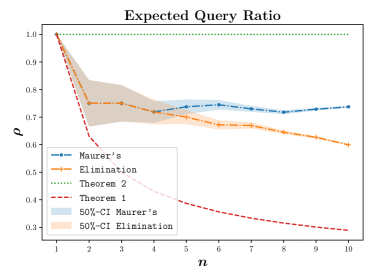
In Figure 12, we plot the bounds above for $n=\{1,\ldots,10\}$, along with two search strategies for $\bm{q}^{*}$ using the Hamming oracle: i) Maurer’s (Maurer, 2009); and ii) search by Elimination which, after response $r^{(i)}$ to query $\bm{q}^{(i)}$, eliminates all binary codes $\bm{q}\in\mathcal{H}$ with $||\bm{q}-\bm{q}^{(i)}||_{H}\neq r^{(i)}$ in an iterative manner. Note that Elimination is a naive technique that is not scalable with $n$.

Theorem 3.

(Optimality of SignHunter) Given $2^{\lceil\log(n)+1\rceil}$ queries and that the directional derivative is well approximated by the finite-difference (Eq. 2 in the main paper), SignHunter is at least as effective as FGSM (Goodfellow et al., 2015) in crafting adversarial examples.

Proof.

Recall that the $i$th coordinate of the gradient sign vector can be recovered as outlined in Eq. 8. From the definition of SignHunter, this is carried out for all the $n$ coordinates after $2^{\lceil\log(n)+1\rceil}$ queries. Put it differently, after $2^{\lceil\log(n)+1\rceil}$ queries, SignHunter has flipped every coordinate alone recovering its sign exactly as shown in Eq. 8. Therefore, the gradient sign vector is fully recovered, and one can employ the FGSM attack to craft an adversarial example. Note that this is under the assumption that our finite difference approximation of the directional derivative (Eq. 2 in the main paper) is good enough (or at least a rank-preserving). ∎

Figure 12: Expected Query Ratios for $n=\{1,\ldots,10\}$ with the noiseless Hamming oracle $\mathcal{O}$.

Appendix D. Experiments Setup

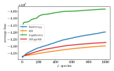
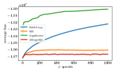
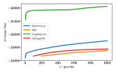
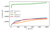
This section outlines the experiments setup as follows. Figure 13 shows the performance of the considered algorithms on a synthetic concave loss function after tuning their hyperparameters. A possible explanation of SignHunter’s superb performance is that the synthetic loss function is well-behaved in terms of its gradient given an image. That is, most of gradient coordinates share the same sign, since pixels tend to have the same values and the optimal value for all the pixels is the same $\frac{\bm{x}_{min}+\bm{x}_{max}}{2}$. Thus, SignHunter will recover the true gradient sign with as few queries as possible (recall the example in Section 4.1 of the main paper). Moreover, given the structure of the synthetic loss function, the optimal loss value is always at the boundary of the perturbation region. The boundary is where SignHunter samples its perturbations. Tables 5, 6, 7, and 8 outline the algorithms’ hyperparameters, while Table 4 describes the general setup for the experiments.

(a) MNIST $\ell_{\infty}$	(b) MNIST $\ell_{2}$
(c) CIFAR10 $\ell_{\infty}$	(d) CIFAR10 $\ell_{2}$
(e) IMAGENET $\ell_{\infty}$	(f) IMAGENET $\ell_{2}$

Figure 13: Tuning testbed for the attacks. A synthetic loss function was used to tune the performance of the attacks over a random sample of 25 images for each dataset and $\ell_{p}$ perturbation constraint. The plots above show the average performance of the tuned attacks on the synthetic loss function $L(\bm{x},y)=-(\bm{x}-\bm{x}^{*})^{T}(\bm{x}-\bm{x}^{*})$, where $\bm{x}^{*}=\frac{\bm{x}_{min}+\bm{x}_{max}}{2}$ using a query limit of $1000$ queries for each image. Note that in all, Bandits_TD outperforms both NES and ZO-SignSGD. Also, we observe the same behavior reported by (Liu et al., 2019) on the fast convergence of ZO-SignSGD compared to NES. We did not tune SignHunter; it does not have any tunable parameters.

Table 4: General setup for all the attacks

	Value
	MNIST		CIFAR10		IMAGENET
	$\ell_{\infty}$	$\ell_{2}$	$\ell_{\infty}$	$\ell_{2}$	$\ell_{\infty}$	$\ell_{2}$
Parameter
$\epsilon$ (allowed perturbation)	0.3	3	12	127	0.05	5
Max allowed queries	10000
Evaluation/Test set size	1000
Data (pixel value) Range	[0,1]		[0,255]		[0,1]

Table 5: Hyperparameters setup for NES

	Value
	MNIST		CIFAR10		IMAGENET
	$\ell_{\infty}$	$\ell_{2}$	$\ell_{\infty}$	$\ell_{2}$	$\ell_{\infty}$	$\ell_{2}$
Hyperparameter
$\delta$ (finite difference probe)	0.1	0.1	2.55	2.55	0.1	0.1
$\eta$ (image $\ell_{p}$ learning rate)	0.1	1	2	127	0.02	2
$q$ (number of finite difference estimations per step)	10	20	20	4	100	50

Table 6: Hyperparameters setup for ZO-SignSGD

	Value
	MNIST		CIFAR10		IMAGENET
	$\ell_{\infty}$	$\ell_{2}$	$\ell_{\infty}$	$\ell_{2}$	$\ell_{\infty}$	$\ell_{2}$
Hyperparameter
$\delta$ (finite difference probe)	0.1	0.1	2.55	2.55	0.1	0.1
$\eta$ (image $\ell_{p}$ learning rate)	0.1	0.1	2	2	0.02	0.004
$q$ (number of finite difference estimations per step)	10	20	20	4	100	50

Table 7: Hyperparameters setup for Bandits_TD

	Value
	MNIST		CIFAR10		IMAGENET
	$\ell_{\infty}$	$\ell_{2}$	$\ell_{\infty}$	$\ell_{2}$	$\ell_{\infty}$	$\ell_{2}$
Hyperparameter
$\eta$ (image $\ell_{p}$ learning rate)	0.03	0.01	5	12	0.01	0.1
$\delta$ (finite difference probe)	0.1	0.1	2.55	2.55	0.1	0.1
$\tau$ (online convex optimization learning rate)	0.001	0.0001	0.0001	1e-05	0.0001	0.1
Tile size (data-dependent prior)	8	10	20	20	50	50
$\zeta$ (bandit exploration)	0.01	0.1	0.1	0.1	0.01	0.1

Table 8: Hyperparameters setup for SignHunter

	Value
	MNIST		CIFAR10		IMAGENET
	$\ell_{\infty}$	$\ell_{2}$	$\ell_{\infty}$	$\ell_{2}$	$\ell_{\infty}$	$\ell_{2}$
Hyperparameter
$\delta$ (finite difference probe)	0.3	3	12	127	0.05	5

Appendix E. Results of Adversarial Black-Box Examples Generation

This section shows results of our experiments in crafting adversarial black-box examples in the form of tables and performance traces, namely Figures 14, 15, and 16; and Tables 9, 10, and 11.

Table 9: Summary of attacks effectiveness on MNIST under $\ell_{\infty}$ and $\ell_{2}$ perturbation constraints, and with a query limit of $10,000$ queries. The Failure Rate $\in[0,1]$ column lists the fraction of failed attacks over $1000$ images. The Avg. # Queries column reports the average number of queries made to the loss oracle only over successful attacks.

	Failure Rate		Avg. # Queries
	$\bm{\ell}_{\infty}$	$\bm{\ell}_{2}$	$\bm{\ell}_{\infty}$	$\bm{\ell}_{2}$
Attack
BanditsTD	$0.68$	$0.59$	$328.00$	$673.16$
NES	$0.63$	$0.63$	$235.07$	$\bf 361.42$
SignHunter	$\bf 0.00$	$\bf 0.04$	$\bf 11.06$	$1064.22$
ZOSignSGD	$0.63$	$0.75$	$157.00$	$881.08$

Table 10: Summary of attacks effectiveness on CIFAR10 under $\ell_{\infty}$ and $\ell_{2}$ perturbation constraints, and with a query limit of $10,000$ queries. The Failure Rate $\in[0,1]$ column lists the fraction of failed attacks over $1000$ images. The Avg. # Queries column reports the average number of queries made to the loss oracle only over successful attacks.

	Failure Rate		Avg. # Queries
	$\bm{\ell}_{\infty}$	$\bm{\ell}_{2}$	$\bm{\ell}_{\infty}$	$\bm{\ell}_{2}$
Attack
BanditsTD	$0.95$	$0.39$	$432.24$	$1201.85$
NES	$0.37$	$0.67$	$312.57$	$\bf 496.99$
SignHunter	$\bf 0.07$	$\bf 0.21$	$\bf 121.00$	$692.39$
ZOSignSGD	$0.37$	$0.80$	$161.28$	$528.35$

Table 11: Summary of attacks effectiveness on IMAGENET under $\ell_{\infty}$ and $\ell_{2}$ perturbation constraints, and with a query limit of $10,000$ queries. The Failure Rate $\in[0,1]$ column lists the fraction of failed attacks over $1000$ images. The Avg. # Queries column reports the average number of queries made to the loss oracle only over successful attacks.

	Failure Rate		Avg. # Queries
	$\bm{\ell}_{\infty}$	$\bm{\ell}_{2}$	$\bm{\ell}_{\infty}$	$\bm{\ell}_{2}$
Attack
BanditsTD	$0.07$	$\bf 0.11$	$1010.05$	$1635.55$
NES	$0.26$	$0.42$	$1536.19$	$1393.86$
SignHunter	$\bf 0.02$	$0.23$	$\bf 578.56$	$1985.55$
ZOSignSGD	$0.23$	$0.52$	$1054.98$	$\bf 931.15$

$\ell_{\infty}$	$\ell_{2}$

Figure 14: Performance curves of attacks on MNIST for $\ell_{\infty}$ (first column) and $\ell_{2}$ (second column) perturbation constraints. Plots of Avg. Loss row reports the loss as a function of the number of queries averaged over all images. The Avg. Hamming Similarity row shows the Hamming similarity of the sign of the attack’s estimated gradient $\hat{\bm{g}}$ with true gradient’s sign $\bm{q}^{*}$, computed as $1-||\operatorname{sign}(\hat{\bm{g}})-\bm{q}^{*}||_{H}/n$ and averaged over all images. Likewise, plots of the Avg. Cosine Similarity row show the normalized dot product of $\hat{\bm{g}}$ and $\bm{g}^{*}$ averaged over all images. The Success Rate row reports the attacks’ cumulative distribution functions for the number of queries required to carry out a successful attack up to the query limit of $10,000$ queries. The Avg. # Queries row reports the average number of queries used per successful image for each attack when reaching a specified success rate: the more effective the attack, the closer its curve is to the bottom right of the plot.

$\ell_{\infty}$	$\ell_{2}$

Figure 15: Performance curves of attacks on CIFAR10 for $\ell_{\infty}$ (first column) and $\ell_{2}$ (second column) perturbation constraints. Plots of Avg. Loss row reports the loss as a function of the number of queries averaged over all images. The Avg. Hamming Similarity row shows the Hamming similarity of the sign of the attack’s estimated gradient $\hat{\bm{g}}$ with true gradient’s sign $\bm{q}^{*}$, computed as $1-||\operatorname{sign}(\hat{\bm{g}})-\bm{q}^{*}||_{H}/n$ and averaged over all images. Likewise, plots of the Avg. Cosine Similarity row show the normalized dot product of $\hat{\bm{g}}$ and $\bm{g}^{*}$ averaged over all images. The Success Rate row reports the attacks’ cumulative distribution functions for the number of queries required to carry out a successful attack up to the query limit of $10,000$ queries. The Avg. # Queries row reports the average number of queries used per successful image for each attack when reaching a specified success rate: the more effective the attack, the closer its curve is to the bottom right of the plot.

$\ell_{\infty}$	$\ell_{2}$

Figure 16: Performance curves of attacks on IMAGENET for $\ell_{\infty}$ (first column) and $\ell_{2}$ (second column) perturbation constraints. Plots of Avg. Loss row reports the loss as a function of the number of queries averaged over all images. The Avg. Hamming Similarity row shows the Hamming similarity of the sign of the attack’s estimated gradient $\hat{\bm{g}}$ with true gradient’s sign $\bm{q}^{*}$, computed as $1-||\operatorname{sign}(\hat{\bm{g}})-\bm{q}^{*}||_{H}/n$ and averaged over all images. Likewise, plots of the Avg. Cosine Similarity row show the normalized dot product of $\hat{\bm{g}}$ and $\bm{g}^{*}$ averaged over all images. The Success Rate row reports the attacks’ cumulative distribution functions for the number of queries required to carry out a successful attack up to the query limit of $10,000$ queries. The Avg. # Queries row reports the average number of queries used per successful image for each attack when reaching a specified success rate: the more effective the attack, the closer its curve is to the bottom right of the plot.

Appendix F. Public Black-Box Challenge Results

Madry’s Lab (MNIST)	Madry’s Lab (CIFAR10)	Ensemble Adversarial Training (IMAGENET)

Figure 17: Performance curves of attacks on the public black-box challenges for MNIST (first column), CIFAR10 (second column) and IMAGENET (third column). Plots of Avg. Loss row reports the loss as a function of the number of queries averaged over all images. The Avg. Hamming Similarity row shows the Hamming similarity of the sign of the attack’s estimated gradient $\hat{\bm{g}}$ with true gradient’s sign $\bm{q}^{*}$, computed as $1-||\operatorname{sign}(\hat{\bm{g}})-\bm{q}^{*}||_{H}/n$ and averaged over all images. Likewise, plots of the Avg. Cosine Similarity row show the normalized dot product of $\hat{\bm{g}}$ and $\bm{g}^{*}$ averaged over all images. The Success Rate row reports the attacks’ cumulative distribution functions for the number of queries required to carry out a successful attack up to the query limit of $5,000$ queries. The Avg. # Queries row reports the average number of queries used per successful image for each attack when reaching a specified success rate: the more effective the attack, the closer its curve is to the bottom right of the plot.

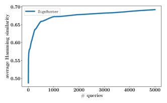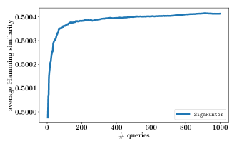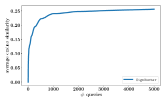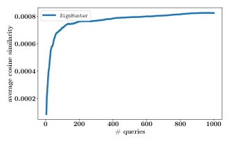Appendix G. Estimating Hamming Oracle

This section illustrates our experiment on the distribution of the magnitudes of gradient coordinates as summarized in Figure 18. How to read the plots: Consider the first histogram in Plot (a) from below; it corresponds to the $1000^{th}$ image from the sampled MNIST evaluation set, plotting the histogram of the values $\{|\partial L(\bm{x},y)/\partial x_{i}|\}_{1\leq i\leq n}$, where the MNIST dataset has dimensionality $n=784$. These values are in the range $[0,0.002]$. Overall, the values are fairly concentrated—with exceptions, in Plot (e) for instance, the magnitudes of the $\sim 400^{th}$ image’s gradient coordinates are spread from $0$ to $\sim 0.055$. Thus, a Monte Carlo estimate of the mean of $\{|\partial L(\bm{x},y)/\partial x_{i}|\}_{1\leq i\leq n}$ would be an appropriate approximation. We release these figures in the form of TensorBoard logs.

	MNIST	CIFAR10	IMAGENET
	\begin{overpic}[width=134.42113pt,unit=1mm,trim=5.01874pt 26.09749pt 0.0pt 20.075pt,clip]{figs/grad_hists/mnist_part_deriv_mag_xo} \put(5.0,-2.0){ \bf\tiny gradient coordinate magnitude} \put(-2.0,7.0){ \rotatebox{90.0}{\bf\tiny\#gradient coordinates}} \put(48.0,4.0){ \rotatebox{90.0}{\bf test image index}} \end{overpic}	\begin{overpic}[width=134.42113pt,unit=1mm,trim=5.01874pt 26.09749pt 0.0pt 20.075pt,clip]{figs/grad_hists/cifar10_part_deriv_mag_xo} \put(5.0,-2.0){ \bf\tiny gradient coordinate magnitude} \put(-2.0,7.0){ \rotatebox{90.0}{\bf\tiny\#gradient coordinates}} \put(48.0,4.0){ \rotatebox{90.0}{\bf test image index}} \end{overpic}	\begin{overpic}[width=134.42113pt,unit=1mm,trim=5.01874pt 26.09749pt 0.0pt 20.075pt,clip]{figs/grad_hists/imagenet_part_deriv_mag_xo} \put(5.0,-2.0){ \bf\tiny gradient coordinate magnitude} \put(-2.0,7.0){ \rotatebox{90.0}{\bf\tiny\#gradient coordinates}} \put(48.0,4.0){ \rotatebox{90.0}{\bf test image index}} \end{overpic}
	(a)	(b)	(c)
	\begin{overpic}[width=134.42113pt,unit=1mm,trim=5.01874pt 26.09749pt 0.0pt 20.075pt,clip]{figs/grad_hists/mnist_part_deriv_mag_xr} \put(5.0,-2.0){ \bf\tiny gradient coordinate magnitude} \put(-2.0,7.0){ \rotatebox{90.0}{\bf\tiny\#gradient coordinates}} \put(48.0,4.0){ \rotatebox{90.0}{\bf test image index}} \end{overpic}	\begin{overpic}[width=134.42113pt,unit=1mm,trim=5.01874pt 26.09749pt 0.0pt 20.075pt,clip]{figs/grad_hists/cifar10_part_deriv_mag_xr} \put(5.0,-2.0){ \bf\tiny gradient coordinate magnitude} \put(-2.0,7.0){ \rotatebox{90.0}{\bf\tiny\#gradient coordinates}} \put(48.0,4.0){ \rotatebox{90.0}{\bf test image index}} \end{overpic}	\begin{overpic}[width=134.42113pt,unit=1mm,trim=5.01874pt 26.09749pt 0.0pt 20.075pt,clip]{figs/grad_hists/imagenet_part_deriv_mag_xr} \put(5.0,-2.0){ \bf\tiny gradient coordinate magnitude} \put(-2.0,7.0){ \rotatebox{90.0}{\bf\tiny\#gradient coordinates}} \put(48.0,4.0){ \rotatebox{90.0}{\bf test image index}} \end{overpic}
	(d)	(e)	(f)

Figure 18: Magnitudes of gradient coordinates are concentrated: Plots (a), (b), and (c) show histograms of the magnitudes of gradient coordinates of the loss function $L(\bm{x},y)$ with respect to the input point (image) $\bm{x}$ for MNIST, CIFAR10, and IMAGENET neural net models over $1000$ images from the corresponding evaluation set, respectively. Plots (d), (e), (f) show the same but at input points (images) sampled randomly within $B_{\infty}(\bm{x},\epsilon)$: the $\ell_{\infty}$-ball of radius $\epsilon=0.3$, $12$, and $0.05$ around the images in Plots (a), (b), and (c), respectively.

References

- Al-Dujaili & Suresh (2017) Al-Dujaili, A. and Suresh, S. Embedded bandits for large-scale black-box optimization. In Thirty-First AAAI Conference on Artificial Intelligence, 2017.
- Al-Dujaili & Suresh (2018) Al-Dujaili, A. and Suresh, S. Multi-objective simultaneous optimistic optimization. Information Sciences, 424:159–174, 2018.
- Al-Dujaili et al. (2015) Al-Dujaili, A., Merciol, F., and Lefèvre, S. Graphbpt: An efficient hierarchical data structure for image representation and probabilistic inference. In International Symposium on Mathematical Morphology and Its Applications to Signal and Image Processing, pp. 301–312. Springer, 2015.
- Al-Dujaili et al. (2018) Al-Dujaili, A., Huang, A., Hemberg, E., and O’Reilly, U.-M. Adversarial deep learning for robust detection of binary encoded malware. In 2018 IEEE Security and Privacy Workshops (SPW), pp. 76–82. IEEE, 2018.
- Bernstein et al. (2018) Bernstein, J., Wang, Y.-X., Azizzadenesheli, K., and Anandkumar, A. signSGD: Compressed optimisation for non-convex problems. In Dy, J. and Krause, A. (eds.), Proceedings of the 35th International Conference on Machine Learning, volume 80 of Proceedings of Machine Learning Research, pp. 560–569, Stockholmsmässan, Stockholm Sweden, 10–15 Jul 2018. PMLR. URL http://proceedings.mlr.press/v80/bernstein18a.html.
- Bhagoji et al. (2017) Bhagoji, A. N., He, W., Li, B., and Song, D. Exploring the space of black-box attacks on deep neural networks. arXiv preprint arXiv:1712.09491, 2017.
- Biggio & Roli (2018) Biggio, B. and Roli, F. Wild patterns: Ten years after the rise of adversarial machine learning. Pattern Recognition, 84:317–331, 2018.
- Biggio et al. (2013) Biggio, B., Corona, I., Maiorca, D., Nelson, B., Šrndić, N., Laskov, P., Giacinto, G., and Roli, F. Evasion attacks against machine learning at test time. In Joint European conference on machine learning and knowledge discovery in databases, pp. 387–402. Springer, 2013.
- Carlini & Wagner (2017) Carlini, N. and Wagner, D. Towards evaluating the robustness of neural networks. In 2017 IEEE Symposium on Security and Privacy (SP), pp. 39–57. IEEE, 2017.
- Chen et al. (2017) Chen, P.-Y., Zhang, H., Sharma, Y., Yi, J., and Hsieh, C.-J. Zoo: Zeroth order optimization based black-box attacks to deep neural networks without training substitute models. In Proceedings of the 10th ACM Workshop on Artificial Intelligence and Security, pp. 15–26. ACM, 2017.
- Chrabaszcz et al. (2018) Chrabaszcz, P., Loshchilov, I., and Hutter, F. Back to basics: Benchmarking canonical evolution strategies for playing atari. arXiv preprint arXiv:1802.08842, 2018.
- Cohen et al. (2019) Cohen, J., Rosenfeld, E., and Kolter, J. Z. Certified adversarial robustness via randomized smoothing. arXiv:1902.02918v1, 2019.
- Demetrio et al. (2019) Demetrio, L., Biggio, B., Giovanni, L., Roli, F., and Alessandro, A. Explaining vulnerabilities of deep learning to adversarial malware binaries. In ITASEC19, 2019.
- Goodfellow et al. (2015) Goodfellow, I., Shlens, J., and Szegedy, C. Explaining and harnessing adversarial examples. In International Conference on Learning Representations, 2015. URL http://arxiv.org/abs/1412.6572.
- Hayes & Danezis (2017) Hayes, J. and Danezis, G. Machine learning as an adversarial service: Learning black-box adversarial examples. CoRR, abs/1708.05207, 2017.
- Huang et al. (2018) Huang, A., Al-Dujaili, A., Hemberg, E., and O’Reilly, U.-M. On visual hallmarks of robustness to adversarial malware. arXiv preprint arXiv:1805.03553, 2018.
- Ilyas et al. (2018) Ilyas, A., Engstrom, L., Athalye, A., and Lin, J. Black-box adversarial attacks with limited queries and information. In Dy, J. and Krause, A. (eds.), Proceedings of the 35th International Conference on Machine Learning, volume 80 of Proceedings of Machine Learning Research, pp. 2137–2146, Stockholmsmässan, Stockholm Sweden, 10–15 Jul 2018. PMLR. URL http://proceedings.mlr.press/v80/ilyas18a.html.
- Ilyas et al. (2019) Ilyas, A., Engstrom, L., and Madry, A. Prior convictions: Black-box adversarial attacks with bandits and priors. In International Conference on Learning Representations, 2019. URL https://openreview.net/forum?id=BkMiWhR5K7.
- Kocsis & Szepesvári (2006) Kocsis, L. and Szepesvári, C. Bandit based monte-carlo planning. In European conference on machine learning, pp. 282–293. Springer, 2006.
- Kurakin et al. (2017) Kurakin, A., Goodfellow, I. J., and Bengio, S. Adversarial machine learning at scale. 2017. URL https://arxiv.org/abs/1611.01236.
- Liu et al. (2019) Liu, S., Chen, P.-Y., Chen, X., and Hong, M. signSGD via zeroth-order oracle. In International Conference on Learning Representations, 2019. URL https://openreview.net/forum?id=BJe-DsC5Fm.
- Liu et al. (2016) Liu, Y., Chen, X., Liu, C., and Song, D. Delving into transferable adversarial examples and black-box attacks. arXiv preprint arXiv:1611.02770, 2016.
- Madry et al. (2017) Madry, A., Makelov, A., Schmidt, L., Tsipras, D., and Vladu, A. Towards deep learning models resistant to adversarial attacks. arXiv preprint arXiv:1706.06083, 2017.
- Maurer (2009) Maurer, P. M. A search strategy using a hamming-distance oracle. 2009.
- Moosavi-Dezfooli et al. (2016) Moosavi-Dezfooli, S.-M., Fawzi, A., and Frossard, P. Deepfool: a simple and accurate method to fool deep neural networks. In Proceedings of the IEEE Conference on Computer Vision and Pattern Recognition, pp. 2574–2582, 2016.
- Munos (2011) Munos, R. Optimistic optimization of a deterministic function without the knowledge of its smoothness. In Advances in neural information processing systems, pp. 783–791, 2011.
- Narodytska & Kasiviswanathan (2017) Narodytska, N. and Kasiviswanathan, S. P. Simple black-box adversarial attacks on deep neural networks. In CVPR Workshops, volume 2, 2017.
- Nelson et al. (2012) Nelson, B., Rubinstein, B. I., Huang, L., Joseph, A. D., Lee, S. J., Rao, S., and Tygar, J. Query strategies for evading convex-inducing classifiers. Journal of Machine Learning Research, 13(May):1293–1332, 2012.
- Papernot et al. (2017) Papernot, N., McDaniel, P., Goodfellow, I., Jha, S., Celik, Z. B., and Swami, A. Practical black-box attacks against machine learning. In Proceedings of the 2017 ACM on Asia Conference on Computer and Communications Security, pp. 506–519. ACM, 2017.
- Salimans et al. (2017) Salimans, T., Ho, J., Chen, X., Sidor, S., and Sutskever, I. Evolution strategies as a scalable alternative to reinforcement learning. arXiv preprint arXiv:1703.03864, 2017.
- Shamir et al. (2019) Shamir, A., Safran, I., Ronen, E., and Dunkelman, O. A simple explanation for the existence of adversarial examples with small hamming distance. arXiv preprint arXiv:1901.10861, 2019.
- Tramèr et al. (2017) Tramèr, F., Kurakin, A., Papernot, N., Goodfellow, I., Boneh, D., and McDaniel, P. Ensemble adversarial training: Attacks and defenses. arXiv preprint arXiv:1705.07204, 2017.
- Tu et al. (2018) Tu, C.-C., Ting, P., Chen, P.-Y., Liu, S., Zhang, H., Yi, J., Hsieh, C.-J., and Cheng, S.-M. Autozoom: Autoencoder-based zeroth order optimization method for attacking black-box neural networks. arXiv preprint arXiv:1805.11770, 2018.
- Vaishampayan (2012) Vaishampayan, V. A. Query matrices for retrieving binary vectors based on the hamming distance oracle. arXiv preprint arXiv:1202.2794, 2012.
- Xiao et al. (2018) Xiao, C., Li, B., Zhu, J.-Y., He, W., Liu, M., and Song, D. Generating adversarial examples with adversarial networks, 2018. URL https://openreview.net/forum?id=HknbyQbC-.
- Zhao (2018) Zhao, Y.-B. Sparse optimization theory and methods. CRC Press, an imprint of Taylor and Francis, Boca Raton, FL, 2018. ISBN 978-1138080942.
- Zheng et al. (2018) Zheng, T., Chen, C., and Ren, K. Distributionally adversarial attack. arXiv preprint arXiv:1808.05537, 2018.