Hyperbolic Discounting and Learning over Multiple Horizons

Abstract

Reinforcement learning (RL) typically defines a discount factor ($\gamma$) as part of the Markov Decision Process. The discount factor values future rewards by an exponential scheme that leads to theoretical convergence guarantees of the Bellman equation. However, evidence from psychology, economics and neuroscience suggests that humans and animals instead have hyperbolic time-preferences ($\frac{1}{1+kt}$ for $k>0$). In this work we revisit the fundamentals of discounting in RL and bridge this disconnect by implementing an RL agent that acts via hyperbolic discounting. We demonstrate that a simple approach approximates hyperbolic discount functions while still using familiar temporal-difference learning techniques in RL. Additionally, and independent of hyperbolic discounting, we make a surprising discovery that simultaneously learning value functions over multiple time-horizons is an effective auxiliary task which often improves over a strong value-based RL agent, Rainbow.

1 Introduction

The standard treatment of the reinforcement learning (RL) problem is the Markov Decision Process (MDP) which includes a discount factor $0\leq\gamma<1$ that exponentially reduces the present value of future rewards (Bellman, 1957; Sutton & Barto, 1998). A reward $r_{t}$ received in $t$-time steps is devalued to $\gamma^{t}r_{t}$, a discounted utility model introduced by Samuelson (1937). This establishes a time-preference for rewards realized sooner rather than later. The decision to exponentially discount future rewards by $\gamma$ leads to value functions that satisfy theoretical convergence properties (Bertsekas, 1995). The magnitude of $\gamma$ also plays a role in stabilizing learning dynamics of RL algorithms (Prokhorov & Wunsch, 1997; Bertsekas & Tsitsiklis, 1996) and has recently been treated as a hyperparameter of the optimization (OpenAI, 2018; Xu et al., 2018).

However, both the magnitude and the functional form of this discounting function implicitly establish priors over the solutions learned. The magnitude of $\gamma$ chosen establishes an effective horizon for the agent, far beyond which rewards are neglected (Kearns & Singh, 2002). This effectively imposes a time-scale of the environment, which may not be accurate. However, less well-known and expanded on later, the exponential discounting of future rewards is consistent with a prior belief that there exists a known constant risk to the agent in the environment (Sozou (1998), Section 3.1). This is a strong assumption that may not be supported in richer environments.

Additionally, discounting future values exponentially and according to a single discount factor $\gamma$ does not harmonize with the measured value preferences in humans and animals (Mazur, 1985; 1997; Ainslie, 1992; Green & Myerson, 2004; Maia, 2009). A wealth of empirical evidence has been amassed that humans, monkeys, rats and pigeons instead discount future returns hyperbolically, where $d_{k}(t)=\frac{1}{1+kt}$, for some positive $k>0$ (Ainslie, 1975; 1992; Mazur, 1985; 1997; Frederick et al., 2002; Green et al., 1981; Green & Myerson, 2004).

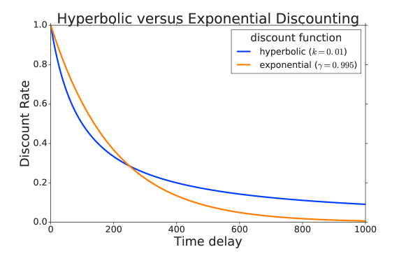
Figure 1: Hyperbolic versus exponential discounting. Humans and animals often exhibit hyperbolic discounts (blue curve) which have shallower discount declines for large horizons. In contrast, RL agents often optimize exponential discounts (orange curve) which drop at a constant rate regardless of how distant the return.

As an example of hyperbolic time-preferences, consider the hypothetical: a stranger approaches with a simple proposition. He offers you $1M immediately with no risk, but if you can wait until tomorrow, he promises you $1.1M dollars. With no further information many are skeptical of this would-be benefactor and choose to receive $1M immediately. Most rightly believe the future promise holds risk. However, in an alternative proposition, he instead promises you $1M in 365 days or $1.1M in 366 days. Under these new terms many will instead choose the $1.1M offer. Effectively, the discount rate has decreased further out, indicating the belief that it is less likely for the promise to be reneged on the 366th day if it were not already broken on the 365th day. Note that discount rates in humans have been demonstrated to vary with the size of the reward so this time-reversal might not emerge for $1 versus $1.1 (Myerson & Green, 1995; Green et al., 1997).

Hyperbolic discounting is consistent with these reversals in time-preferences (Green et al., 1994). Exponential discounting, on the other hand, always remains consistent between these choices and was shown in Strotz (1955) to be the only time-consistent sliding discount function. This discrepancy between the time-preferences of animals from the exponential discounted measure of value might be presumed irrational. However, Sozou (1998) demonstrates that this behavior is mathematically consistent with the agent maintaining some uncertainty over the hazard rate in the environment. In this formulation, rewards are discounted based on the possibility the agent will succumb to a risk and will thus not survive to collect them. Hazard rate, defined in Section 3, measures the per-time-step risk the agent incurs as it acts in the environment.

Hazard and its associated discount function. Common RL environments are also characterized by risk, but in a narrower sense. In deterministic environments like the original Arcade Learning Environment (ALE) (Bellemare et al., 2013) stochasticity is often introduced through techniques like no-ops (Mnih et al., 2015) and sticky actions (Machado et al., 2018) where the action execution is noisy. Physics simulators may have noise and the randomness of the policy itself induces risk. But even with these stochastic injections the risk to reward emerges in a more restricted sense. Episode-to-episode risk may vary as the value function and resulting policy evolve. States once safely navigable may become dangerous through catastrophic forgetting (McCloskey & Cohen, 1989; French, 1999) or through exploration the agent may venture to new dangerous areas of the state space. However, this is still a narrow manifestation of risk as the environment is generally stable and repetitive. In Section 4 we show that a prior distribution reflecting the uncertainty over the hazard rate, has an associated discount function in the sense that an MDP with either this hazard distribution or the discount function, has the same value function for all policies. This equivalence implies that learning policies with a discount function can be interpreted as making them robust to the associated hazard distribution. Thus, discounting serves as a tool to ensure that policies deployed in the real world perform well even under risks they were not trained under.

Hyperbolic discounting from TD-learning algorithms. We propose an algorithm that approximates hyperbolic discounting while building on successful Q-learning (Watkins & Dayan, 1992) tools and their associated theoretical guarantees. We show learning many Q-values, each discounting exponentially with a different discount factor $\gamma$, can be aggregated to approximate hyperbolic (and other non-exponential) discount factors. We demonstrate the efficacy of our approximation scheme in our proposed Pathworld environment which is characterized both by an uncertain per-time-step risk to the agent. The agent must choose which risky path to follow but it stands to gain a higher reward the longer, riskier paths. A conceptually similar situation might arise for a foraging agent balancing easily realizable, small meals versus more distant, fruitful meals. The setup is described in further detail in Section 7. We then consider higher-dimensional RL agents in the ALE, where we measure the benefits of our technique. Our approximation mirrors the work of Kurth-Nelson & Redish (2009); Redish & Kurth-Nelson (2010) which empirically demonstrates that modeling a finite set of $\mu$Agents simultaneously can approximate hyperbolic discounting function which is consistent with fMRI studies (Tanaka et al., 2004; Schweighofer et al., 2008). Our method extends to other non-hyperbolic discount functions and uses deep neural networks to model the different Q-values from a shared representation.

Surprisingly and in addition to enabling new discounting schemes, we observe that learning a set of Q-values is beneficial as an auxiliary task (Jaderberg et al., 2016). Adding this multi-horizon auxiliary task often improves over strong baselines including C51 (Bellemare et al., 2017) and Rainbow (Hessel et al., 2018) in the ALE (Bellemare et al., 2013).

The paper is organized as follows. Section 3 recounts how a prior belief of the risk in the environment can imply a specific discount function. Section 4 formalizes hazard in MDPs. In Section 5 we demonstrate that hyperbolic (and other) discounting rates can be computed by Q-learning (Watkins & Dayan, 1992) over multiple horizons, that is, multiple discount functions $\gamma$. We then provide a practical approach to approximating these alternative discount schemes in Section 6. We demonstrate the efficacy of our approximation scheme in the Pathworld environment in Section 7 and then go on to consider the high-dimensional ALE setting in Sections 7, 9. We conclude with ablation studies, discussion and commentary on future research directions.

This work questions the RL paradigm of learning policies through a single discount function which exponentially discounts future rewards through two contributions:

1. Hyperbolic (and other non-exponential)-agent. A practical approach for training an agent which discounts future rewards by a hyperbolic (or other non-exponential) discount function and acts according to this.

2. Multi-horizon auxiliary task. A demonstration of multi-horizon learning over many $\gamma$ simultaneously as an effective auxiliary task.

2 Related Work

Hyperbolic discounting in economics. Hyperbolic discounting is well-studied in the field of economics (Sozou, 1998; Dasgupta & Maskin, 2005). Dasgupta and Maskin (2005) proposes a softer interpretation than Sozou (1998) (which produces a per-time-step of death via the hazard rate) and demonstrates that uncertainty over the timing of rewards can also give rise to hyperbolic discounting and preference reversals, a hallmark of hyperbolic discounting. However, though alternative motivations for hyperbolic discounting exist we build upon Sozou (1998) for its clarity and simplicity.

Hyperbolic discounting was initially presumed to not lend itself to TD-based solutions (Daw & Touretzky, 2000) but the field has evolved on this point. Maia (2009) proposes solution directions that find models that discount quasi-hyperbolically even though each learns with exponential discounting (Loewenstein, 1996) but reaffirms the difficulty. Finally, Alexander and Brown (2010) proposes hyperbolically discounted temporal difference (HDTD) learning by making connections to hazard. However, this approach introduces two additional free parameters to adjust for differences in reward-level.

Behavior RL and hyperbolic discounting in neuroscience. TD-learning has long been used for modeling behavioral reinforcement learning (Montague et al., 1996; Schultz et al., 1997; Sutton & Barto, 1998). TD-learning computes the error as the difference between the expected value and actual value (Sutton & Barto, 1998; Daw, 2003) where the error signal emerges from unexpected rewards. However, these computations traditionally rely on exponential discounting as part of the estimate of the value which disagrees with empirical evidence in humans and animals (Strotz, 1955; Mazur, 1985; 1997; Ainslie, 1975; 1992). Hyperbolic discounting has been proposed as an alternative to exponential discounting though it has been debated as an accurate model (Kacelnik, 1997; Frederick et al., 2002). Naive modifications to TD-learning to discount hyperbolically present issues since the simple forms are inconsistent (Daw & Touretzky, 2000; Redish & Kurth-Nelson, 2010) RL models have been proposed to explain behavioral effects of humans and animals (Fu & Anderson, 2006; Rangel et al., 2008) but Kurth-Nelson & Redish (2009) demonstrated that distributed exponential discount factors can directly model hyperbolic discounting. This work proposes the $\mu$Agent, an agent that models the value function with a specific discount factor $\gamma$. When the distributed set of $\mu$Agent’s votes on the action, this was shown to approximate hyperbolic discounting well in the adjusting-delay assay experiments (Mazur, 1987). Using the hazard formulation established in Sozou (1998), we demonstrate how to extend this to other non-hyperbolic discount functions and demonstrate the efficacy of using a deep neural network to model the different Q-values from a shared representation.

Towards more flexible discounting in reinforcement learning. RL researchers have recently adopted more flexible versions beyond a fixed discount factor (Feinberg & Shwartz, 1994; Sutton, 1995; Sutton et al., 2011; White, 2017). Optimal policies are studied in Feinberg & Shwartz (1994) where two value functions with different discount factors are used. Introducing the discount factor as an argument to be queried for a set of timescales is considered in both Horde (Sutton et al., 2011) and $\gamma$-nets (Sherstan et al., 2018). Reinke et al. (2017) proposes the Average Reward Independent Gamma Ensemble framework which imitates the average return estimator.

Lattimore and Hutter (2011) generalizes the original discounting model through discount functions that vary with the age of the agent, expressing time-inconsistent preferences as in hyperbolic discounting. The need to increase training stability via effective horizon was addressed in François-Lavet, Fonteneau, and Ernst (2015) who proposed dynamic strategies for the discount factor $\gamma$. Meta-learning approaches to deal with the discount factor have been proposed in Xu, van Hasselt, and Silver (2018). Finally, Pitis (2019) characterizes rational decision making in sequential processes, formalizing a process that admits a state-action dependent discount rates. This body of work suggests growing tension between the original MDP formulation with a fixed $\gamma$ and future research directions.

Operating over multiple time scales has a long history in RL. Sutton (1995) generalizes the work of Singh (1992) and Dayan and Hinton (1993) to formalize a multi-time scale TD learning model theory. Previous work has been explored on solving MDPs with multiple reward functions and multiple discount factors though these relied on separate transition models (Feinberg & Shwartz, 1999; Dolgov & Durfee, 2005). Edwards, Littman, and Isbell (2015) considers decomposing a reward function into separate components each with its own discount factor. In our work, we continue to model the same rewards, but now model the value over different horizons. Recent work in difficult exploration games demonstrates the efficacy of two different discount factors (Burda et al., 2018) one for intrinsic rewards and one for extrinsic rewards. Finally, and concurrent with this work, Romoff et al. (2019) proposes the TD$(\Delta)$-algorithm which breaks a value function into a series of value functions with smaller discount factors.

Auxiliary tasks in reinforcement learning. Finally, auxiliary tasks have been successfully employed and found to be of considerable benefit in RL. Suddarth and Kergosien (1990) used auxiliary tasks to facilitate representation learning. Building upon this, work in RL has consistently demonstrated benefits of auxiliary tasks to augment the low-information coming from the environment through extrinsic rewards (Lample & Chaplot, 2017; Mirowski et al., 2016), (Jaderberg et al., 2016; Veeriah et al., 2018; Sutton et al., 2011)

3 Belief of Risk Implies a Discount Function

Sozou (1998) formalizes time preferences in which future rewards are discounted based on the probability that the agent will not survive to collect them due to an encountered risk or hazard.

Definition 3.1.

Survival $s(t)$ is the probability of the agent surviving until time $t$.

$$s(t)=P(\text{agent is alive}|\text{at time}\;t)$$ (1)

A future reward $r_{t}$ is less valuable presently if the agent is unlikely to survive to collect it. If the agent is risk-neutral, the present value of a future reward $r_{t}$ received at time-$t$ should be discounted by the probability that the agent will survive until time $t$ to collect it, $s(t)$.

$$v(r_{t})=s(t)r_{t}$$ (2)

Consequently, if the agent is certain to survive, $s(t)=1$, then the reward is not discounted per Equation 2. From this it is then convenient to define the hazard rate.

Definition 3.2.

Hazard rate $h(t)$ is the negative rate of change of the log-survival at time $t$

$$h(t)=-\frac{d}{dt}\text{ln}s(t)$$ (3)

or equivalently expressed as $h(t)=-\frac{ds(t)}{dt}\frac{1}{s(t)}$. Therefore the environment is considered hazardous at time $t$ if the log survival is decreasing sharply.

Sozou (1998) demonstrates that the prior belief of the risk in the environment implies a specific discounting function. When the risk occurs at a known constant rate than the agent should discount future rewards exponentially. However, when the agent holds uncertainty over the hazard rate then hyperbolic and alternative discounting rates arise.

3.1 Known Hazard Implies Exponential Discount

We recover the familiar exponential discount function in RL based on a prior assumption that the environment has a known constant hazard. Consider a known hazard rate of $h(t)=\lambda\ \geq 0$. Definition 3 sets a first order differential equation $\lambda=-\frac{d}{dt}\text{ln}s(t)=-\frac{ds(t)}{dt}\frac{1}{s(t)}$. The solution for the survival rate is $s(t)=e^{-\lambda t}$ which can be related to the RL discount factor $\gamma$

$$s(t)=e^{-\lambda t}=\gamma^{t}$$ (4)

This interprets $\gamma$ as the per-time-step probability of the episode continuing. This also allows us to connect the hazard rate $\lambda\in[0,\infty]$ to the discount factor $\gamma\in[0,1)$.

$$\gamma=e^{-\lambda}$$ (5)

As the hazard increases $\lambda\rightarrow\infty$, then the corresponding discount factor becomes increasingly myopic $\gamma\rightarrow 0$. Conversely, as the environment hazard vanishes, $\lambda\rightarrow 0$, the corresponding agent becomes increasingly far-sighted $\gamma\rightarrow 1$.

In RL we commonly choose a single $\gamma$ which is consistent with the prior belief that there exists a known constant hazard rate $\lambda=-\text{ln}(\gamma)$. We now relax the assumption that the agent holds this strong prior that it exactly knows the true hazard rate. From a Bayesian perspective, a looser prior allows for some uncertainty in the underlying hazard rate of the environment which we will see in the following section.

3.2 Uncertain Hazard Implies Non-Exponential Discount

We may not always be so confident of the true risk in the environment and instead reflect this underlying uncertainty in the hazard rate through a hazard prior $p(\lambda)$. Our survival rate is then computed by weighting specific exponential survival rates defined by a given $\lambda$ over our prior $p(\lambda)$

$$s(t)=\int_{\lambda=0}^{\infty}p(\lambda)e^{-\lambda t}d\lambda$$ (6)

Sozou (1998) shows that under an exponential prior of hazard $p(\lambda)=\frac{1}{k}\text{exp}(-\lambda/k)$ the expected survival rate for the agent is hyperbolic

$$s(t)=\frac{1}{1+kt}\equiv\Gamma_{k}(t)$$ (7)

We denote the hyperbolic discount by $\Gamma_{k}(t)$ to make the connection to $\gamma$ in reinforcement learning explicit. Further, Sozou (1998) shows that different priors over hazard correspond to different discount functions. We reproduce two figures in Figure 2 showing the correspondence between different hazard rate priors and the resultant discount functions. The common approach in RL is to maintain a delta-hazard (black line) which leads to exponential discounting of future rewards. Different priors lead to non-exponential discount functions.

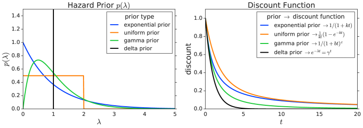
Figure 2: We reproduce two figures from Sozou (1998). There is a correspondence between hazard rate priors and the resulting discount function. In RL, we typically discount future rewards exponentially which is consistent with a Dirac delta prior (black line) on the hazard rate indicating no uncertainty of hazard rate. However, this is a special case and priors with uncertainty over the hazard rate imply new discount functions. All priors have the same mean hazard rate $\mathbb{E}[p(\lambda)]=1$.

4 Hazard in MDPs

To study MDPs with hazard distributions and general discount functions we introduce two modifications. The hazardous MDP now is defined by the tuple $<\mathcal{S},\mathcal{A},R,P,\mathcal{H},d>$. In standard form, the state space $\mathcal{S}$ and the action space $\mathcal{A}$ may be discrete or continuous. The learner observes samples from the environment transition probability $P(s_{t+1}|s_{t},a_{t})$ for going from $s_{t}\in\mathcal{S}$ to $s_{t+1}\in\mathcal{S}$ given $a_{t}\in\mathcal{A}$. We will consider the case where $P$ is a sub-stochastic transition function, which defines an episodic MDP. The environment emits a bounded reward $r:\mathcal{S}\times\mathcal{A}\rightarrow\left[r_{min},r_{max}\right]$ on each transition. In this work we consider non-infinite episodic MDPs.

The first difference is that at the beginning of each episode, a hazard $\lambda\in[0,\infty)$ is sampled from the hazard distribution $\mathcal{H}$. This is equivalent to sampling a continuing probability $\gamma=e^{-\lambda}$. During the episode, the hazard modified transition function will be $P_{\lambda}$, in that $P_{\lambda}(s^{\prime}|s,a)=e^{-\lambda}P(s^{\prime}|s,a)$. The second difference is that we now consider a general discount function $d(t)$. This differs from the standard approach of exponential discounting in RL with $\gamma$ according to $d(t)=\gamma^{t}$, which is a special case.

This setting makes a close connection to partially observable Markov Decision Process (POMDP) (Kaelbling et al., 1998) where one might consider $\lambda$ as an unobserved variable. However, the classic POMDP definition contains an explicit discount function $\gamma$ as part of it’s definition which does not appear here.

A policy $\pi:\mathcal{S}\rightarrow\mathcal{A}$ is a mapping from states to actions. The state action value function $Q_{\pi}^{\mathcal{H},d}(s,a)$ is the expected discounted rewards after taking action $a$ in state $s$ and then following policy $\pi$ until termination.

$$Q^{\mathcal{H},d}_{\pi}(s,a)=\mathbb{E}_{\lambda}\mathbb{E}_{\pi,P_{\lambda}}\left[\sum_{t=0}^{\infty}d(t)R(s_{t},a_{t})|s_{0}=s,a_{0}=a\right]$$ (8)

where $\lambda\sim\mathcal{H}$ and $\mathbb{E}_{\pi,P_{\lambda}}$ implies that $s_{t+1}\sim P_{\lambda}(\cdot|s_{t},a_{t})$ and $a_{t}\sim\pi(\cdot|s_{t})$.

4.1 Equivalence Between Hazard and Discounting

In the hazardous MDP setting we observe the same connections between hazard and discount functions delineated in Section 3. This expresses an equivalence between the value function of an MDP with a discount and MDP with a hazard distribution.

For example, there exists an equivalence between the exponential discount function $d(t)=\gamma^{t}$ to the undiscounted case where the agent is subject to a $(1-\gamma)$ per time-step of dying (Lattimore & Hutter, 2011). The typical Q-value (left side of Equation 9) is when the agent acts in an environment without hazard $\lambda=0$ or $\mathcal{H}=\delta(0)$ and discounts future rewards according to $d(t)=\gamma^{t}=e^{-\lambda t}$ which we denote as $Q_{\pi}^{\delta(0),\gamma^{t}}(s,a)$. The alternative Q-value (right side of Equation 9) is when the agent acts under hazard rate $\lambda=-\ln\gamma$ but does not discount future rewards which we denote as $Q_{\pi}^{\delta(-\ln\gamma),1}(s,a)$.

$$Q_{\pi}^{\delta(0),\gamma^{t}}(s,a)=Q_{\pi}^{\delta(-\ln\gamma),1}(s,a)\;\forall\;\pi,s,a.$$ (9)

where $\delta(x)$ denotes the Dirac delta distribution at $x$. This follows from $P_{\lambda}(s^{\prime}|s,a)=e^{-\lambda}P(s^{\prime}|s,a)$

$$\mathbb{E}_{\pi,P}\left[\sum_{t=0}^{\infty}\gamma^{t}R(s_{t},a_{t})|s_{0}=s,a_{0}=a\right] =\mathbb{E}_{\pi,P}\left[\sum_{t=0}^{\infty}e^{-\lambda t}R(s_{t},a_{t})|s_{0}=s,a_{0}=a\right]$$

$$=\mathbb{E}_{\pi,P_{\lambda}}\left[\sum_{t=0}^{\infty}R(s_{t},a_{t})|s_{0}=s,a_{0}=a\right]$$

Following Section 3 we also show a similar equivalence between hyperbolic discounting and the specific hazard distribution $p_{k}(\lambda)=\frac{1}{k}\text{exp}(-\lambda/k)$, where again, $\lambda\in[0,\infty)$ in Appendix A.

$$Q_{\pi}^{\delta(0),\Gamma_{k}}(s,a)=Q_{\pi}^{p_{k},1}(s,a)$$

For notational brevity later in the paper, we will omit the explicit hazard distribution $\mathcal{H}$-superscript if the environment is not hazardous.

5 Computing Hyperbolic Q-Values From Exponential Q-Values

We show how one can re-purpose exponentially-discounted Q-values to compute hyperbolic (and other-non-exponential) discounted Q-values. The central challenge with using non-exponential discount strategies is that most RL algorithms use some form of TD learning (Sutton, 1988). This family of algorithms exploits the Bellman equation (Bellman, 1958) which, when using exponential discounting, relates the value function at one state with the value at the following state.

$$Q_{\pi}^{\gamma^{t}}(s,a)=\mathbb{E}_{\pi,P}[R(s,a)+\gamma Q_{\pi}(s^{\prime},a^{\prime})]$$ (10)

where expectation $\mathbb{E}_{\pi,P}$ denotes sampling $a\sim\pi(\cdot|s)$, $s^{\prime}\sim P(\cdot|s,a)$, and $a^{\prime}\sim\pi(\cdot|s^{\prime})$.

Being able to reuse the literature on TD methods without being constrained to exponential discounting is thus an important challenge.

5.1 Computing Hyperbolic $Q$-Values

Let’s start with the case where we would like to estimate the value function where rewards are discounted hyperbolically instead of the common exponential scheme. We refer to the hyperbolic Q-values as $Q^{\Gamma}_{\pi}$ below in Equation 12

$$Q^{\Gamma_{k}}_{\pi}(s,a)= \mathbb{E}_{\pi}\left[\Gamma_{k}(1)R(s_{1},a_{1})+\Gamma_{k}(2)R(s_{2},a_{2})+\cdots\biggr{|}s,a\right]$$ (11)

$$= \mathbb{E}_{\pi}\left[\sum_{t}\Gamma_{k}(t)R(s_{t},a_{t})\biggr{|}s,a\right]$$ (12)

We may relate the hyperbolic $Q^{\Gamma}_{\pi}$-value to the values learned through standard $Q$-learning. To do so, notice that the hyperbolic discount $\Gamma_{t}$ can be expressed as the integral of a certain function $f(\gamma,t)$ for $\gamma=[0,1)$ in Equation 13.

$$\int_{\gamma=0}^{1}\gamma^{kt}d\gamma=\frac{1}{1+kt}=\Gamma_{k}(t)$$ (13)

The integral over this specific function $f(\gamma,t)=\gamma^{kt}$ yields the desired hyperbolic discount factor $\Gamma_{k}(t)$ by considering an infinite set of exponential discount factors $\gamma$ over its domain $\gamma\in[0,1)$. We visualize the hyperbolic discount factors $\frac{1}{1+t}$ (consider $k=1$) for the first few time-steps $t$ in Figure 3.

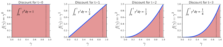
Figure 3: From left to right we consider the first four time-steps ($t=0,1,2,3$) of the function $\gamma^{t}$ (shown in blue) over the valid range. The integral (red) of $\gamma^{t}$ at time $t$ equals the hyperbolic discount function $1/(1+t)$ shown in each subplot. Time $t=0$ is not discounted since the integral of $\gamma^{0}=1$ from 0 to 1 is 1. Then $t=1$ is discounted by $\frac{1}{2}$, $t=2$ is discounted by $t=\frac{1}{3}$ and so on. For illustration, the black dotted vertical line indicates the discount that we would use for each time-step if we considered only a single discount factor $\gamma=0.9$.

Recognize that the integrand $\gamma^{kt}$ is the standard exponential discount factor which suggests a connection to standard Q-learning (Watkins & Dayan, 1992). This suggests that if we could consider an infinite set of $\gamma$ then we can combine them to yield hyperbolic discounts for the corresponding time-step $t$. We build on this idea of modeling many $\gamma$ throughout this work.

We employ Equation 13 and return to the task of computing hyperbolic Q-values $Q^{\Gamma}_{\pi}(s,a)$

$$Q^{\Gamma}_{\pi}(s,a)= \mathbb{E}_{\pi}\left[\sum_{t}\Gamma_{k}(t)R(s_{t},a_{t})\biggr{|}s,a\right]$$ (14)

$$= \mathbb{E}_{\pi}\left[\sum_{t}\left(\int_{\gamma=0}^{1}\gamma^{kt}d\gamma\right)R(s_{t},a_{t})\biggr{|}s,a\right]$$ (15)

$$= \int_{\gamma=0}^{1}\mathbb{E}_{\pi}\left[\sum_{t}R(s_{t},a_{t})(\gamma^{k})^{t}\biggr{|}s,a\right]d\gamma$$ (16)

$$= \int_{\gamma=0}^{1}Q^{(\gamma^{k})^{t}}_{\pi}(s,a)d\gamma$$ (17)

where $\Gamma_{k}(t)$ has been replaced on the first line by $\left(\int_{\gamma=0}^{1}\gamma^{kt}d\gamma\right)$ and the exchange is valid if $\sum_{t=0}^{\infty}\gamma^{kt}r_{t}<\infty$. This shows us that we can compute the $Q^{\Gamma}_{\pi}$-value according to hyperbolic discount factor by considering an infinite set of $Q^{\gamma^{k}}_{\pi}$-values computed through standard $Q$-learning. Examining further, each $\gamma\in[0,1)$ results in TD-errors learned for a new $\gamma^{k}$. For values of $k<1$, which extends the horizon of the hyperbolic discounting, this would result in larger $\gamma$.

5.2 Generalizing to Other Non-Exponential $Q$-Values

Equation 13 computes hyperbolic discount functions but its origin was not mathematically motivated. We consider here an alternative scheme to deduce ways to model hyperbolic as well as different discount schemes through integrals of $\gamma$.

Lemma 5.1.

Let $Q_{\pi}^{\mathcal{H},\gamma}(s,a)$ be the state action value function under exponential discounting in a hazardous MDP $<\mathcal{S},\mathcal{A},R,P,\mathcal{H},\gamma^{t}>$ and let $Q_{\pi}^{\mathcal{H},d}(s,a)$ refer to the value function in the same MDP except for new discounting $<\mathcal{S},\mathcal{A},R,P,\mathcal{H},d>$. If there exists a function $w:[0,1]\to\mathbb{R}$ such that

$$d(t)=\int_{0}^{1}w(\gamma)\gamma^{t}d\gamma$$ (18)

which we will refer to as the exponential weighting condition, then

$$Q_{\pi}^{\mathcal{H},d}(s,a)=\int_{0}^{1}w(\gamma)Q_{\pi}^{\mathcal{H},\gamma}(s,a)d\gamma$$ (19)

Proof.

Applying the condition on $d$,

$$Q_{\pi}^{\mathcal{H},d}(s,a) =\mathbb{E}_{\lambda}\mathbb{E}_{\pi,P_{\lambda}}\left[\sum_{t=0}^{\infty}\left(\int_{0}^{1}w(\gamma)\gamma^{t}d\gamma\right)R(s_{t},a_{t})|s_{0}=s,a_{0}=a\right]$$ (20)

$$=\int_{0}^{1}\mathbb{E}_{\lambda}\mathbb{E}_{\pi,P_{\lambda}}w(\gamma)\left[\sum_{t=0}^{\infty}\gamma^{t}R(s_{t},a_{t})|s_{0}=s,a_{0}=a\right]d\gamma$$ (21)

$$=\int_{0}^{1}w(\gamma)Q_{\pi}^{\mathcal{H},\gamma}(s,a)d\gamma$$ (22)

∎

where again the exchange is valid if $\sum_{t=0}^{\infty}\gamma^{t}R(s_{t},a_{t})<\infty$. We can now see that the exponential weighting condition is satisfied for hyperbolic discounting and a list of other discounting that we might want to consider.

For instance, the hyperbolic discount can also be expressed as the integral of a different function $f(\gamma,t)$ for $\gamma=[0,1)$ in Equation 23.

$$\frac{1}{k}\int_{\gamma=0}^{1}\gamma^{1/k+t-1}d\gamma=\frac{1}{1+kt}$$ (23)

As before, an integral over a function $f^{\prime}(\gamma,t)=\frac{1}{k}\gamma^{1/k+t-1}=w(\gamma)\gamma^{t}$ yields the desired hyperbolic discount factor $\Gamma_{k}(t)$. This integral can be derived by recognizing Equation 6 as the Laplace transform of the prior $\mathcal{H}=p(\lambda)$ and then applying a change of variables $\gamma=e^{-\lambda}$. Computing hyperbolic and other discount functions is demonstrated in detail in Appendix B. We summarize in Table 1 how a particular hazard prior $p(\lambda)$ can be computed via integrating over specific weightings $w(\gamma)$ and the corresponding discount function.

	$\mathcal{H}=p(\lambda)$	$d(t)$	$w(\gamma)$
Dirac Delta Prior	$\delta(\lambda-k)$	$e^{-kt}(=(\gamma_{k})^{t})$	$\frac{1}{\gamma}\delta(-\ln\gamma-k)$
Exponential Prior	$\frac{1}{k}e^{-\lambda/k}$	$\frac{1}{1+kt}$	$\frac{1}{k}\gamma^{1/k-1}$
Uniform Prior	$\begin{cases}\frac{1}{k},&\text{if}\ \lambda\in[0,k]\\ 0,&\text{otherwise}\end{cases}$	$\frac{1}{kt}\left(1-e^{-kt}\right)$	$\begin{cases}\frac{1}{k}\gamma^{-1},&\text{if}\ \gamma\in[e^{-k},1]\\ 0,&\text{otherwise}\end{cases}$

Table 1: Different hazard priors $\mathcal{H}=p(\lambda)$ can be alternatively expressed through weighting exponential discount functions $\gamma^{t}$ by $w(\gamma)$. This table matches different hazard distributions to their associated discounting function and the weighting function per Lemma 5.1. The typical case in RL is a Dirac Delta Prior over hazard rate $\delta(\lambda-k)$. We only show this in detail for completeness; one would not follow such a convoluted path to arrive back at an exponential discount but this approach holds for richer priors. The derivations can be found in the Appendix B.

6 Approximating Hyperbolic $Q$-Values

Section 5 describes an equivalence between hyperbolically-discounted Q-values and integrals of exponentially-discounted Q-values requiring evaluating an infinite set of value functions. We now present a practical approach to approximate discounting $\Gamma(t)=\frac{1}{1+kt}$ using standard $Q$-learning (Watkins & Dayan, 1992).

6.1 Approximating the Discount Factor Integral

To avoid estimating an infinite number of $Q^{\gamma}_{\pi}$-values we introduce a free hyperparameter ($n_{\gamma}$) which is the total number of $Q^{\gamma}_{\pi}$-values to consider, each with their own $\gamma$. We use a practically-minded approach to choose $\mathcal{G}$ that emphasizes evaluating larger values of $\gamma$ rather than uniformly choosing points and empirically performs well as seen in Section 7.

$$\mathcal{G}=[\gamma_{0},\gamma_{1},\cdots,\gamma_{n_{\gamma}}]$$ (24)

Our approach is described in Appendix C. Each $Q_{\pi}^{\gamma_{i}}$ computes the discounted sum of returns according to that specific discount factor $Q^{\gamma_{i}}_{\pi}(s,a)=\mathbb{E}_{\pi}\left[\sum_{t}(\gamma_{i})^{t}r_{t}|s_{0}=s,a_{0}=a\right]$.

We previously proposed two equivalent approaches for computing hyperbolic Q-values, but for simplicity we consider the one presented in Lemma 5.1. The set of $Q$-values permits us to estimate the integral through a Riemann sum (Equation 25) which is described in further detail in Appendix D.

$$Q_{\pi}^{\Gamma}(s,a)= \int_{0}^{1}w(\gamma)Q_{\pi}^{\gamma}(s,a)d\gamma$$ (25)

$$\approx \sum_{\gamma_{i}\in\mathcal{G}}(\gamma_{i+1}-\gamma_{i})\;w(\gamma_{i})\;Q_{\pi}^{\gamma_{i}}(s,a)$$ (26)

where we estimate the integral through a lower bound. We consolidate this entire process in Figure 4 where we show the full process of rewriting the hyperbolic discount rate, hyperbolically-discounted Q-value, the approximation and the instantiated agent. This approach is similar to that of Kurth-Nelson & Redish (2009) where each $\mu$Agent models a specific discount factor $\gamma$. However, this differs in that our final agent computes a weighted average over each Q-value rather than a sampling operation of each agent based on a $\gamma$-distribution.

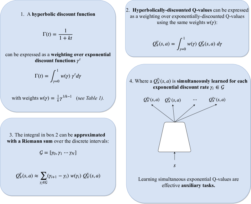
Figure 4: Summary of our approach to approximating hyperbolic (and other non-exponential) Q-values via a weighted sum of exponentially-discounted Q-vaulues.

7 Pathworld Experiments

7.1 When to Discount Hyperbolically?

The benefits of hyperbolic discounting will be greatest under:

1. Uncertain hazard. The hazard-rate characterizing the environment is not known. For instance, an unobserved hazard-rate variable $\lambda$ is drawn independently at the beginning of each episode from $\mathcal{H}=p(\lambda)$.

2. Non-trivial intertemporal decisions. The agent faces non-trivial intertemporal decision. A non-trivial decision is one between smaller nearby rewards versus larger distant rewards..

In the absence of both properties we would not expect any advantage to discounting hyperbolically. As described before, if there is a single-true hazard rate $\lambda_{\text{env}}$, than an optimal $\gamma^{*}=e^{-\lambda_{\text{env}}}$ exists and future rewards should be discounted exponentially according to it. Further, without non-trivial intertemporal trade-offs which would occur if there is one path through the environment with perfect alignment of short- and long-term objectives, all discounting schemes will yield the same optimal policy.

7.2 Pathworld Details

We note two sources for discounting rewards in the future: time delay and survival probability (Section 4). In Pathworld of 5, we train to maximize hyperbolically discounted returns ($\sum_{t}\Gamma_{k}(t)R(s_{t},a_{t})$) under no hazard ($\mathcal{H}=\delta(\lambda-0)$) but then evaluate the undiscounted returns $d(t)=1.0\;\forall\;t$ with the paths subject to hazard $\mathcal{H}=\frac{1}{k}\text{exp}(-\lambda/k)$. Through this procedure, we are able to train an agent that is robust to hazards in the environment.

The agent makes one decision in Pathworld (Figure 5): which of the $N$ paths to investigate. Once a path is chosen, the agent continues until it reaches the end or until it dies. This is similar to a multi-armed bandit, with each action subject to dynamic risk. The paths vary quadratically in length with the index $d(i)=i^{2}$ but the rewards increase linearly with the path index $r(i)=i$. This presents a non-trivial decision for the agent. At deployment, an unobserved hazard $\lambda\sim\mathcal{H}$ is drawn and the agent is subject to a per-time-step risk of dying of $(1-e^{-\lambda})$. This environment differs from the adjusting-delay procedure presented by Mazur (1987) and then later modified by Kurth-Nelson & Redish (2009). Rather then determining time-preferences through varaible-timing of rewards, we determine time-preferences through risk to the reward.

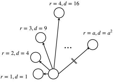
Figure 5: The Pathworld. Each state (white circle) indicates the accompanying reward $r$ and the distance from the starting state $d$. From the start state, the agent makes a single action: which which path to follow to the end. Longer paths have a larger rewards at the end, but the agent incurs a higher risk on a longer path.

7.3 Results in Pathworld

Figure 7 validates that our approach well-approximates the true hyperbolic value of each path when the hazard prior matches the true distribution. Agents that discount exponentially according to a single $\gamma$ (as is commonly the case in RL) incorrectly value the paths.

[0.55]

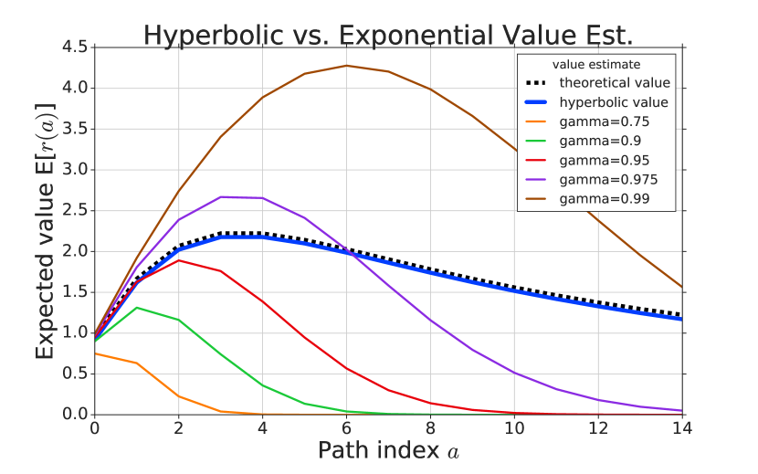
Figure 6: In each episode of Pathworld an unobserved hazard $\lambda\sim p(\lambda)$ is drawn and the agent is subject to a total risk of the reward not being realized of $(1-e^{-\lambda})^{d(a)}$ where $d(a)$ is the path length. When the agent’s hazard prior matches the true hazard distribution, the value estimate agrees well with the theoretical value. Exponential discounts for many $\gamma$ fail to well-approximate the true value as seen to the right in Table 7.

Discount function	MSE
hyperbolic value	0.002
$\gamma$=0.975	0.566
$\gamma$=0.95	1.461
$\gamma$=0.9	2.253
$\gamma$=0.99	2.288
$\gamma$=0.75	2.809

Figure 7: The average mean squared error (MSE) over each of the paths in Figure 7 showing that our approximation scheme well-approximates the true value-profile.

We examine further the failure of exponential discounting in this hazardous setting. For this environment, the true hazard parameter in the prior was $k=0.05$ (i.e. $\lambda\sim 20\text{exp}(-\lambda/0.05)$). Therefore, at deployment, the agent must deal with dynamic levels of risk and faces a non-trivial decision of which path to follow. Even if we tune an agent’s $\gamma=0.975$ such that it chooses the correct arg-max path, it still fails to capture the functional form (Figure 7) and it achieves a high error over all paths (Table 7). If the arg-max action was not available or if the agent was proposed to evaluate non-trivial intertemporal decisions, it would act sub-optimally.

In the next two experiments we consider the more realistic case where the agent’s prior over hazard does not exactly match the environment true hazard rate. In Figure 9 we consider the case that the agent still holds an exponential prior but has the wrong coefficient $k$ and in Figure 11 we consider the case where the agent still holds an exponential prior but the true hazard is actually drawn from a uniform distribution with the same mean.

[0.55]

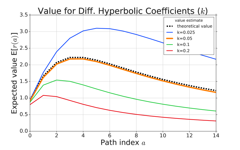
Figure 8: Case when the hazard coefficient $k$ does not match that environment hazard. Here the true hazard coefficient is $k=0.05$, but we compute values for hyperbolic agents with mismatched priors in range $k=[0.025,0.05,0.1,0.2]$. Predictably, the mismatched priors result in a higher prediction error of value but performs more reliably than exponential discounting, resulting in a cumulative lower error. Numerical results in Table 9.

Discount function	MSE
k=0.05	0.002
k=0.1	0.493
k=0.025	0.814
k=0.2	1.281

Figure 9: The average mean squared error (MSE) over each of the paths in Figure 9. As the prior is further away from the true value of $k=0.05$, the error increases. However, notice that the errors for large factor-of-2 changes in $k$ result in generally lower errors than if the agent had considered only a single exponential discount factor $\gamma$ as in Table 7.

[0.55]

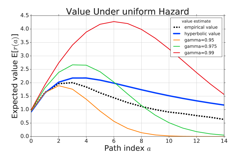
Figure 10: If the true hazard rate is now drawn according to a uniform distribution (with the same mean as before) the original hyperbolic discount matches the functional form better than exponential discounting. Numerical results in Table 11.

Discount function	MSE
hyperbolic value	0.235
$\gamma=0.975$	0.266
$\gamma=0.95$	0.470
$\gamma=0.99$	4.029

Figure 11: The average mean squared error (MSE) over each of the paths in Figure 11 when the underlying hazard is drawn according to a uniform distribution. We find that hyperbolic discounting results is more robust to hazards drawn from a uniform distribution than exponential discounting.

Through these two validating experiments, we demonstrate the robustness of estimating hyperbolic discounted Q-values in the case when the environment presents dynamic levels of risk and the agent faces non-trivial decisions. Hyperbolic discounting is preferable to exponential discounting even when the agent’s prior does not precisely match the true environment hazard rate distribution, by coefficient (Figure 9) or by functional form (Figure 11).

8 Atari 2600 Experiments

With our approach validated in Pathworld, we now move to the high-dimensional environment of Atari 2600, specifically, ALE. We use the Rainbow variant from Dopamine (Castro et al., 2018) which implements three of the six considered improvements from the original paper: distributional RL, predicting n-step returns and prioritized replay buffers.

The agent (Figure 12) maintains a shared representation $h(s)$ of state, but computes $Q$-value logits for each of the $N$ $\gamma_{i}$ via $Q_{\pi}^{(i)}(s,a)=f(W_{i}h(s)+b_{i})$ where $f(\cdot)$ is a ReLU-nonlinearity (Nair & Hinton, 2010) and $W_{i}$ and $b_{i}$ are the learnable parameters of the affine transformation for that head.

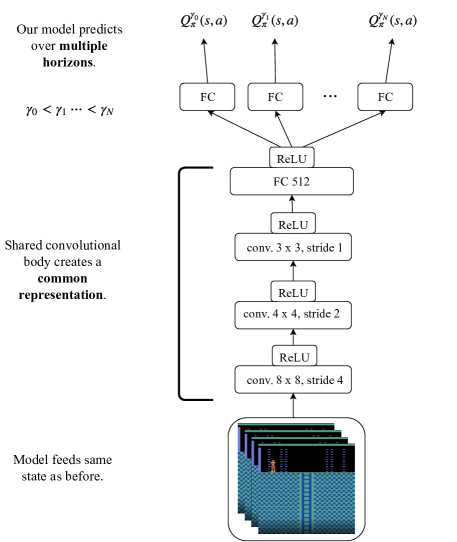
Figure 12: Multi-horizon model predicts $Q$-values for $n_{\gamma}$ separate discount functions thereby modeling different effective horizons. Each $Q$-value is a lightweight computation, an affine transformation off a shared representation. By modeling over multiple time-horizons, we now have the option to construct policies that act according to a particular value or a weighted combination.

We provide details on the hyperparameters in Appendix G. We consider the performance of the hyperbolic agent built on Rainbow (referred to as Hyper-Rainbow) on a random subset of Atari 2600 games in Figure 13.

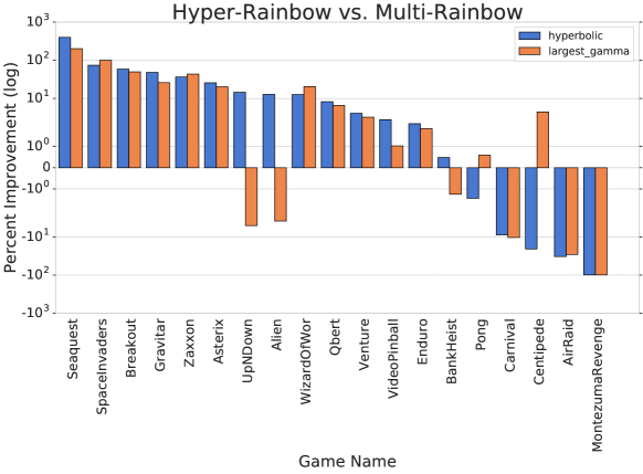
Figure 13: We compare the Hyper-Rainbow (in blue) agent versus the Multi-Rainbow (orange) agent on a random subset of 19 games from ALE (3 seeds each). For each game, the percentage performance improvement for each algorithm against Rainbow is recorded. There is no significant difference whether the agent acts according to hyperbolically-discounted (Hyper-Rainbow) or exponentially-discounted (Multi-Rainbow) Q-values suggesting the performance improvement in ALE emerges from the multi-horizon auxiliary task.

We find that the Hyper-Rainbow agent (blue) performs very well, often improving over the strong-baseline Rainbow agent. On this subset of 19 games, we find that it improves upon 14 games and in some cases, by large margins. However, in Section 9 we seek a more complete understanding of the underlying driver of this improvement in ALE through an ablation study.

9 Multi-Horizon Auxiliary Task Results

To dissect the ALE improvements, recognize that Hyper-Rainbow changes two properties from the base Rainbow agent:

1. Behavior policy. The agent acts according to hyperbolic Q-values computed by our approximation described in Section 6

2. Learn over multiple horizons. The agent simultaneously learns Q-values over many $\gamma$ rather than a Q-value for a single $\gamma$

The second modification can be regarded as introducing an auxiliary task (Jaderberg et al., 2016). Therefore, to attribute the performance of each properly we construct a Rainbow agent augmented with the multi-horizon auxiliary task (referred to as Multi-Rainbow and shown in orange) but have it still act according to the original policy. That is, Multi-Rainbow acts to maximize expected rewards discounted by a fixed $\gamma_{action}$ but now learns over multiple horizons as shown in Figure 12.

We find that the Multi-Rainbow agent performs nearly as well on these games, suggesting the effectiveness of this as a stand-alone auxiliary task. This is not entirely unexpected given the rather special-case of hazard exhibited in ALE through sticky-actions (Machado et al., 2018).

We examine further and investigate the performance of this auxiliary task across the full Arcade Learning Environment (Bellemare et al., 2017) using the recommended evaluation by (Machado et al., 2018). Doing so we find empirical benefits of the multi-horizon auxiliary task on the Rainbow agent as shown in Figure 14.

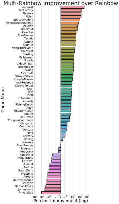
Figure 14: Performance improvement over Rainbow using the multi-horizon auxiliary task in Atari Learning Environment (3 seeds each).

9.1 Analysis and Ablation Studies

To understand the interplay of the multi-horizon auxiliary task with other improvements in deep RL, we test a random subset of 10 Atari 2600 games against improvements in Rainbow (Hessel et al., 2018). On this set of games we measure a consistent improvement with multi-horizon C51 (Multi-C51) in 9 out of the 10 games over the base C51 agent (Bellemare et al., 2017) in Figure 15.

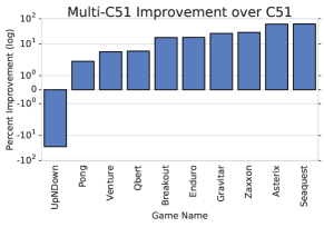
(a) Multi-C51

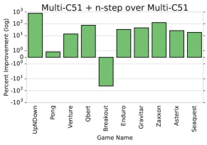
(b) Multi-C51 + n-step

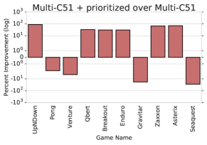
(c) Multi-C51 + priority

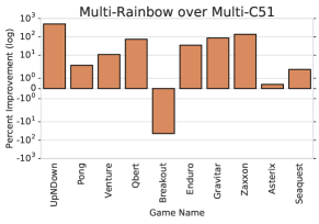
(d) Multi-Rainbow (=Multi-C51 + n-step + priority)

Figure 15: Measuring the Rainbow improvements on top of the Multi-C51 baseline on a subset of 10 games in the Arcade Learning Environment (3 seeds each). On this subset, we find that the multi-horizon auxiliary task interfaces well with n-step methods (top right) but poorly with a prioritized replay buffer (bottom left).

Figure 15 indicates that the current implementation of Multi-Rainbow does not generally build successfully on the prioritized replay buffer. On the subset of ten games considered, we find that four out of ten games (Pong, Venture, Gravitar and Zaxxon) are negatively impacted despite (Hessel et al., 2018) finding it to be of considerable benefit and specifically beneficial in three out of these four games (Venture was not considered). The current prioritization scheme simply averaged the temporal-difference errors over all $Q$-values to establish priority. Alternative prioritization schemes are offering encouraging preliminary results (Appendix E).

10 Discussion

This work builds on a body of work that questions one of the basic premises of RL: one should maximize the exponentially discounted returns via a single discount factor. By learning over multiple horizons simultaneously, we have broadened the scope of our learning algorithms. Through this we have shown that we can enable acting according to new discounting schemes and that learning multiple horizons is a powerful stand-alone auxiliary task. Our method well-approximates hyperbolic discounting and performs better in hazardous MDP distributions. This may be viewed as part of an algorithmic toolkit to model alternative discount functions.

11 Future Work

There is growing interest in the time-preferences of RL agents. Through this work we have considered models of a constant, albeit uncertain, hazard rate $\lambda$. This moves beyond the canonical RL approach of fixing a single $\gamma$ which implicitly holds no uncertainty on the value of $\lambda$ but this still does not fully capture all aspects of risk since the hazard rate may be a function of time. Further, hazard may not be an intrinsic property of the environment but a joint property of both the policy and the environment. If an agent purses a policy leading to dangerous state distributions then it will naturally be subject to higher hazards and vice-versa. We would therefore expect an interplay between time-preferences and policy. This is not simple to deal with but recent work proposing state-action dependent discounting (Pitis, 2019) may provide a formalism for more general time-preference schemes.

Appendix A Equivalence of Hyperbolic Discounting and Exponential Hazard

Following Section 3 we also show a similar equivalence between hyperbolic discounting and the specific hazard distribution $p_{k}(\lambda)=\frac{1}{k}\text{exp}(-\lambda/k)$, where again, $\lambda\in[0,\infty)$

$$Q_{\pi}^{\delta(0),\Gamma_{k}}(s,a) =\mathbb{E}_{\pi,P_{0}}\left[\sum_{t=0}^{\infty}\Gamma_{k}(t)R(s_{t},a_{t})|s_{0}=s,a_{0}=a\right]$$

$$=\mathbb{E}_{\pi,P_{0}}\left[\sum_{t=0}^{\infty}\left(\int_{\lambda=0}^{\infty}p_{k}(\lambda)e^{-\lambda t}d\lambda\right)R(s_{t},a_{t})|s_{0}=s,a_{0}=a\right]$$

$$=\int_{\lambda=0}^{\infty}p_{k}(\lambda)\mathbb{E}_{\pi,P_{0}}\left[\sum_{t=0}^{\infty}e^{-\lambda t}R(s_{t},a_{t})|s_{0}=s,a_{0}=a\right]d\lambda$$

$$=\mathbb{E}_{\lambda\sim p_{k}(\cdot)}\mathbb{E}_{\pi,P_{0}}\left[\sum_{t=0}^{\infty}e^{-\lambda t}R(s_{t},a_{t})|s_{0}=s,a_{0}=a\right]$$

$$=\mathbb{E}_{\lambda\sim p_{k}(\cdot)}\mathbb{E}_{\pi,P_{\lambda}}\left[\sum_{t=0}^{\infty}R(s_{t},a_{t})|s_{0}=s,a_{0}=a\right]$$

$$=Q_{\pi}^{p_{k},1}(s,a)$$

Where the first step uses Equation 7. This equivalence implies that discount factors can be used to learn policies that are robust to hazards.

Appendix B Alternative Discount Functions

We expand upon three special cases to see how functions $f(\gamma,t)=w(\gamma)\gamma^{t}$ may be related to different discount functions $d(t)$.

Three cases:

1. Delta hazard prior: $p(\lambda)=\delta(\lambda-k)$

2. Exponential hazard prior: $p(\lambda)=\frac{1}{k}e^{-\lambda/k}$

3. Uniform hazard prior: $p(\lambda)=\frac{1}{k}$ for $\lambda\in[0,k]$

For the three cases we begin with the Laplace transform on the prior $p(\lambda)=\int_{\lambda=0}^{\infty}p(\lambda)e^{-\lambda t}d\lambda$ and then chnage the variables according to the relation between $\gamma=e^{-\lambda}$, Equation 5.

B.1 Delta Hazard Prior

A delta prior $p(\lambda)=\delta(\lambda-k)$ on the hazard rate is consistent with exponential discounting.

$$\int_{\lambda=0}^{\infty}p(\lambda)e^{-\lambda t}d\lambda =\int_{\lambda=0}^{\infty}\delta(\lambda-k)e^{-\lambda t}d\lambda$$

$$=e^{-kt}$$

where $\delta(\lambda-k)$ is a Dirac delta function defined over variable $\lambda$ with value $k$. The change of variable $\gamma=e^{-\lambda}$ (equivalently $\lambda=-\ln\gamma$) yields differentials $d\lambda=-\frac{1}{\gamma}d\gamma$ and the limits $\lambda=0\rightarrow\gamma=1$ and $\lambda=\infty\rightarrow\gamma=0$. Additionally, the hazard rate value $\lambda=k$ is equivalent to the $\gamma=e^{-k}$.

$$d(t) =\int_{\lambda=0}^{\infty}p(\lambda)e^{-\lambda t}d\lambda$$

$$=\int_{\gamma=1}^{0}\delta(-\ln\gamma-k)\gamma^{t}\left(-\frac{1}{\gamma}d\gamma\right)$$

$$=\int_{\gamma=0}^{1}\delta(-\ln\gamma-k)\gamma^{t-1}d\gamma$$

$$=e^{-kt}$$

$$=\gamma_{k}^{t}$$

where we define a $\gamma_{k}=e^{-k}$ to make the connection to standard RL discounting explicit. Additionally and reiterating, the use of a single discount factor, in this case $\gamma_{k}$, is equivalent to the prior that a single hazard exists in the environment.

B.2 Exponential Hazard Prior

Again, the change of variable $\gamma=e^{-\lambda}$ yields differentials $d\lambda=-\frac{1}{\gamma}d\gamma$ and the limits $\lambda=0\rightarrow\gamma=1$ and $\lambda=\infty\rightarrow\gamma=0$.

$$\int_{\lambda=0}^{\infty}p(\lambda)e^{-\lambda t}d\lambda =\int_{\gamma=1}^{0}p(-\text{ln}\gamma)\gamma^{t}\left(-\frac{1}{\gamma}d\gamma\right)$$

$$=\int_{\gamma=0}^{1}p(-\text{ln}\gamma)\gamma^{t-1}d\gamma$$

where $p(\cdot)$ is the prior. With the exponential prior $p(\lambda)=\frac{1}{k}\text{exp}(-\lambda/k)$ and by substituting $\lambda=-\text{ln}\gamma$ we verify Equation 23

$$\int_{0}^{1}\frac{1}{k}\text{exp}(\ln\gamma/k)\gamma^{t-1}d\gamma =\frac{1}{k}\int_{0}^{1}\text{exp}(\text{ln}\gamma^{1/k})\gamma^{t-1}d\gamma$$

$$=\frac{1}{k}\int_{0}^{1}\gamma^{1/k+t-1}d\gamma$$

$$=\frac{1}{k}\frac{1}{\frac{1}{k}+t}\gamma^{1/k+t}\biggr{\rvert}_{\gamma=0}^{1}$$

$$=\frac{1}{1+kt}$$

B.3 Uniform Hazard Prior

Finally if we hold a uniform prior over hazard, $\frac{1}{k}$ for $\lambda\in[0,k]$ then Sozou (1998) shows the Laplace transform yields

$$d(t)= \int_{0}^{\infty}p(\lambda)e^{-\lambda t}d\lambda$$

$$= \frac{1}{k}\int_{0}^{k}e^{-\lambda t}d\lambda$$

$$= -\frac{1}{kt}e^{-\lambda t}\biggr{|}_{\lambda=0}^{k}$$

$$= \frac{1}{kt}\left(1-e^{-kt}\right)$$

Use the same change of variables to relate this to $\gamma$. The bounds of the integral become $\lambda=0\rightarrow\gamma=1$ and $\lambda=k\rightarrow\gamma=e^{-k}$.

$$d(t)= -\frac{1}{k}\int_{\gamma=1}^{e^{-k}}\gamma^{t-1}d\gamma$$

$$= \frac{1}{kt}\gamma^{t}\biggr{|}_{\gamma=e^{-k}}^{1}$$

$$= \frac{1}{kt}\left(1-e^{-kt}\right)$$

which recovers the discounting scheme.

Appendix C Determining the $\gamma$ Interval

We provide further detail for which $\gamma$ we choose to model and motivation why. We choose a $\gamma_{\text{max}}$ which is the largest $\gamma$ to learn through Bellman updates. If we are using $k$ as the hyperbolic coefficient in Equation 7 and we are approximating the integral with $n_{\gamma}$ our $\gamma_{\text{max}}$ would be

$$\gamma_{\text{max}}=\left(1-b^{n_{\gamma}}\right)^{k}$$ (27)

However, allowing $\gamma_{\text{max}}\rightarrow 1$ get arbitrarily close to 1 may result in learning instabilities Bertsekas (1995). Therefore we compute an exponentiation base of $b=\text{exp}(\text{ln}(1-\gamma_{\text{max}}^{1/k})/n_{\gamma})$ which bounds our $\gamma_{\text{max}}$ at a known stable value. This induces an approximation error which is described more in Appendix F.

Appendix D Estimating Hyperbolic Coefficients

As discussed, we can estimate the hyperbolic discount in two different ways. We illustrate the resulting estimates here and resulting approximations. We use lower-bound Riemann sums in both cases for simplicity but more sophisticated integral estimates exist.

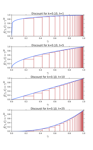
(a) Our approach.

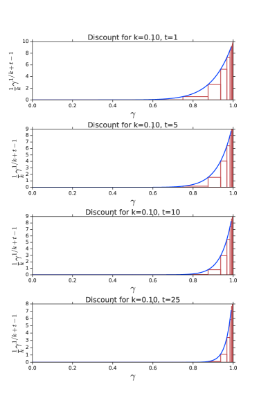
(b) Alternative approach.

Figure 16: Comparison of hyperbolic coefficient integral estimation between the two approaches.
(a) We approximate the integral of the function $\gamma^{kt}$ via a lower estimate of rectangles at specific $\gamma$-values. The sum of these rectangles approximates the hyperbolic discounting scheme $1/(1+kt)$ for time $t$.
(b) Alternative form for approximating hyperbolic coefficients which is sharply peaked as $\gamma\rightarrow 1$ which led to larger errors in estimation under our initial techniques.

As noted earlier, we considered two different integrals for computed the hyperbolic coefficients. Under the form derived by the Laplace transform, the integrals are sharply peaked as $\gamma\rightarrow 1$. The difference in integrals is visually apparent comparing in Figure 16.

Appendix E Performance of Different Replay Buffer Prioritization Scheme

As found through our ablation study in Figure 15, the Multi-Rainbow auxiliary task interacted poorly with the prioritized replay buffer when the TD-errors were averaged evenly across all heads. As an alternative scheme, we considered prioritizing according to the largest $\gamma$, which is also the $\gamma$ defining the $Q$-values by which the agent acts.

The (preliminary) results of this new prioritization scheme is in Figure 17.

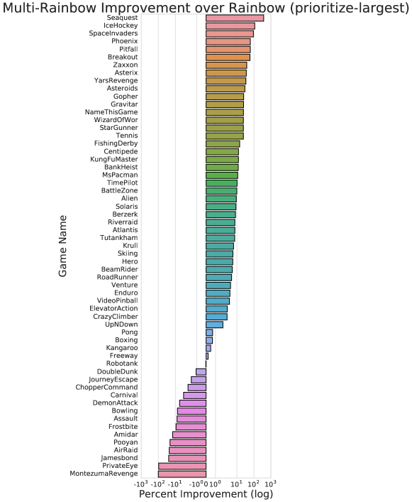
Figure 17: The (preliminary) performance improvement over Rainbow using the multi-horizon auxiliary task in Atari Learning Environment when we instead prioritize according to the TD-errors computed from the largest $\gamma$ (3 seeds each).

To this point, there is evidence that prioritizing according to the TD-errors generated by the largest gamma is a better strategy than averaging.

Appendix F Approximation Errors

Instead of evaluating the upper bound of Equation 23 at 1 we evaluate at $\gamma_{\text{max}}$ which yields $\gamma_{\text{max}}^{kt}/(1+kt)$. Our approximation induces an error in the approximation of the hyperbolic discount.

[0.6]

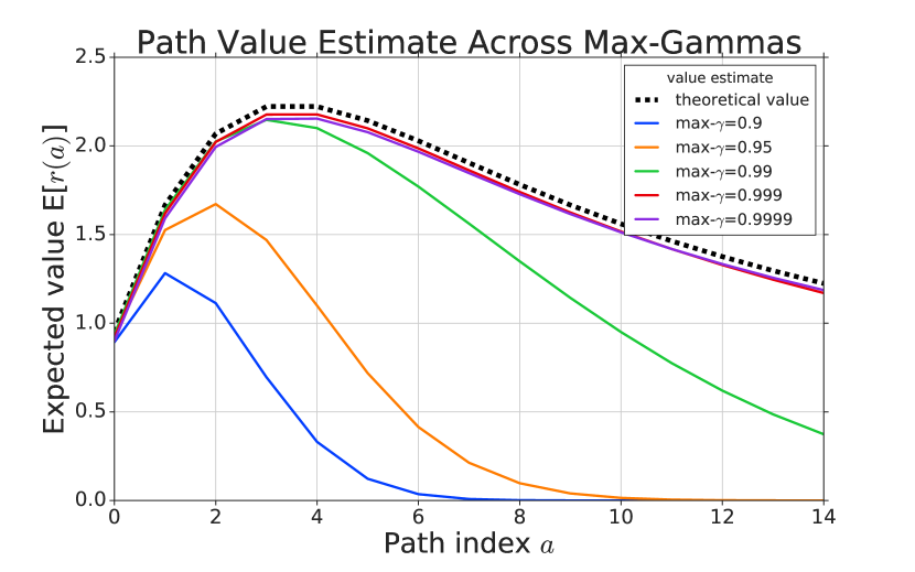
Figure 18: By instead evaluating our integral up to $\gamma_{\text{max}}$ rather than to 1, we induce an approximation error which increases with $t$. Numerical results in Table 19.

Discount function	MSE
max-$\gamma$=0.999	0.002
max-$\gamma$=0.9999	0.003
max-$\gamma$=0.99	0.233
max-$\gamma$=0.95	1.638
max-$\gamma$=0.9	2.281

Figure 19: The average mean squared error (MSE) over each of the paths in Figure 19.

This approximation error in the Riemann sum increases as the $\gamma_{\text{max}}$ decreases as evidenced by Figure 19. When the maximum value of $\gamma_{\text{max}}\rightarrow 1$ then the approximation becomes more accurate as supported in Table 19 up to small random errors.

Appendix G Hyperparameters

For all our experiments in DQN Mnih et al. (2015), C51 Bellemare et al. (2017) and Rainbow Hessel et al. (2018), we benchmark against the baselines set by Castro et al. (2018) and we use the default hyperparameters for each of the respective algorithms. That is, our Multi-agent uses the same optimization, learning rates, and hyperparameters as it’s base class.

Hyperparameter	Value
Runner.sticky_actions	Sticky actions prob 0.25
Runner.num_iterations	200
Runner.training_steps	250000
Runner.evaluation_steps	125000
Runner.max_steps_per_episode	27000
WrappedPrioritizedReplayBuffer.replay_capacity	1000000
WrappedPrioritizedReplayBuffer.batch_size	32
RainbowAgent.num_atoms	51
RainbowAgent.vmax	10.
RainbowAgent.update_horizon	3
RainbowAgent.min_replay_history	20000
RainbowAgent.update_period	4
RainbowAgent.target_update_period	8000
RainbowAgent.epsilon_train	0.01
RainbowAgent.epsilon_eval	0.001
RainbowAgent.epsilon_decay_period	250000
RainbowAgent.replay_scheme	’prioritized’
RainbowAgent.tf_device	’/gpu:0’
RainbowAgent.optimizer	@tf.train.AdamOptimizer()
tf.train.AdamOptimizer.learning_rate	0.0000625
tf.train.AdamOptimizer.epsilon	0.00015
HyperRainbowAgent.number_of_gamma	10
HyperRainbowAgent.gamma_max	0.99
HyperRainbowAgent.hyp_exponent	0.01
HyperRainbowAgent.acting_policy	’largest_gamma’

Table 2: Configurations for the Multi-C51 and Multi-Rainbow used with Dopamine Castro et al. (2018).

Appendix H Auxiliary Task Results

Final results of the multi-horizon auxiliary task on Rainbow (Multi-Rainbow) in Table 3.

Game Name	DQN	C51	Rainbow	Multi-Rainbow
AirRaid	8190.3	9191.2	16941.2	12659.5
Alien	2666.0	2611.4	3858.9	3917.2
Amidar	1306.0	1488.2	2805.7	2477.0
Assault	1661.6	2079.0	3815.9	3415.1
Asterix	3772.5	15289.5	19789.2	24385.6
Asteroids	844.7	1241.5	1524.1	1654.5
Atlantis	935784.0	894862.0	890592.0	923276.7
BankHeist	723.5	863.4	1209.0	1132.0
BattleZone	20508.5	28323.2	42911.1	38827.1
BeamRider	6326.4	6070.6	7026.7	7610.9
Berzerk	590.3	538.3	864.0	879.1
Bowling	40.3	49.8	68.8	62.9
Boxing	83.3	83.5	98.8	99.3
Breakout	146.6	254.1	123.9	162.5
Carnival	4967.9	4917.1	5211.8	5072.2
Centipede	3419.9	8068.9	6878.0	6946.6
ChopperCommand	3084.5	6230.4	13415.1	13942.9
CrazyClimber	113992.2	146072.3	151454.9	160161.0
DemonAttack	7229.2	8485.1	19738.0	14780.9
DoubleDunk	-4.5	2.7	22.6	21.9
ElevatorAction	2434.3	73416.0	81958.0	85633.3
Enduro	895.0	1652.9	2290.1	2337.5
FishingDerby	12.4	16.6	44.5	45.1
Freeway	26.3	33.8	33.8	33.8
Frostbite	1609.6	4522.8	8988.5	7929.7
Gopher	6685.8	8301.1	11749.6	13664.6
Gravitar	339.1	709.8	1293.0	1638.7
Hero	17548.5	34117.8	47545.4	50141.8
IceHockey	-5.0	-3.3	2.6	6.3
Jamesbond	618.3	816.5	1263.8	773.4
JourneyEscape	-2604.2	-1759.1	-818.1	-1002.9
Kangaroo	13118.1	9419.7	13794.0	13930.6
Krull	6558.0	7232.3	6292.5	6645.7
KungFuMaster	26161.2	27089.5	30169.6	31635.2
MontezumaRevenge	2.6	1087.5	501.3	800.3
MsPacman	3664.0	3986.2	4254.2	4707.3
NameThisGame	7808.1	12934.0	9658.9	11045.9
Phoenix	5893.4	6577.3	8979.0	23720.3
Pitfall	-11.8	-5.3	0.0	0.0
Pong	17.4	19.7	20.3	20.6
Pooyan	3800.8	3771.2	6347.7	4670.0
PrivateEye	2051.8	19868.5	21591.4	888.9
Qbert	11011.4	11616.6	19733.2	20817.4
Riverraid	12502.4	13780.4	21624.2	21421.2
RoadRunner	40903.3	49039.8	56527.4	55613.0
Robotank	62.5	64.7	67.9	67.2
Seaquest	2512.4	38242.7	11791.5	64985.0
Skiing	-15314.9	-17996.7	-17792.9	-15603.3
Solaris	2062.7	2788.0	3061.9	3139.9
SpaceInvaders	1976.0	4781.9	4927.9	8802.1
StarGunner	47174.3	35812.4	58630.5	72943.2
Tennis	-0.0	22.2	0.0	0.0
TimePilot	3862.5	8562.7	12486.1	14421.7
Tutankham	141.1	253.1	255.6	264.9
UpNDown	10977.6	9844.8	42572.5	50862.3
Venture	88.0	1430.7	1612.4	1639.9
VideoPinball	222710.4	594468.5	651413.1	650701.1
WizardOfWor	3150.8	3633.8	8992.3	9318.9
YarsRevenge	25372.0	12534.2	47183.8	49929.4
Zaxxon	5199.9	7509.8	15906.2	21921.3

Table 3: Multi-Rainbow agent returns versus the DQN, C51 and Rainbow agents of Dopamine Castro et al. (2018).

References

- Ainslie (1975) George Ainslie. Specious reward: a behavioral theory of impulsiveness and impulse control. Psychological bulletin, 82(4):463, 1975.
- Ainslie (1992) George Ainslie. Picoeconomics: The strategic interaction of successive motivational states within the person. Cambridge University Press, 1992.
- Alexander & Brown (2010) William H Alexander and Joshua W Brown. Hyperbolically discounted temporal difference learning. Neural computation, 22(6):1511–1527, 2010.
- Bellemare et al. (2013) Marc G Bellemare, Yavar Naddaf, Joel Veness, and Michael Bowling. The arcade learning environment: An evaluation platform for general agents. Journal of Artificial Intelligence Research, 47:253–279, 2013.
- Bellemare et al. (2017) Marc G Bellemare, Will Dabney, and Rémi Munos. A distributional perspective on reinforcement learning. arXiv preprint arXiv:1707.06887, 2017.
- Bellman (1957) Richard Bellman. A markovian decision process. Journal of Mathematics and Mechanics, 6(5):679–684, 1957.
- Bellman (1958) Richard Bellman. On a routing problem. Quarterly of applied mathematics, 16(1):87–90, 1958.
- Bertsekas (1995) Dimitri P Bertsekas. Neuro-dynamic programming: an overview. 1995.
- Bertsekas & Tsitsiklis (1996) Dimitri P Bertsekas and John N Tsitsiklis. Neuro-dynamic programming, volume 5. Athena Scientific Belmont, MA, 1996.
- Burda et al. (2018) Yuri Burda, Harrison Edwards, Amos Storkey, and Oleg Klimov. Exploration by random network distillation. arXiv preprint arXiv:1810.12894, 2018.
- Castro et al. (2018) Pablo Samuel Castro, Subhodeep Moitra, Carles Gelada, Saurabh Kumar, and Marc G. Bellemare. Dopamine: A research framework for deep reinforcement learning. CoRR, abs/1812.06110, 2018. URL http://arxiv.org/abs/1812.06110.
- Dasgupta & Maskin (2005) Partha Dasgupta and Eric Maskin. Uncertainty and hyperbolic discounting. American Economic Review, 95(4):1290–1299, 2005.
- Daw (2003) Nathaniel D Daw. Reinforcement learning models of the dopamine system and their behavioral implications. PhD thesis, Carnegie Mellon University, 2003.
- Daw & Touretzky (2000) Nathaniel D Daw and David S Touretzky. Behavioral considerations suggest an average reward td model of the dopamine system. Neurocomputing, 32:679–684, 2000.
- Dayan & Hinton (1993) Peter Dayan and Geoffrey E Hinton. Feudal reinforcement learning. In Advances in neural information processing systems, pp. 271–278, 1993.
- Dolgov & Durfee (2005) Dmitri Dolgov and Edmund Durfee. Stationary deterministic policies for constrained mdps with multiple rewards, costs, and discount factors. Ann Arbor, 1001:48109, 2005.
- Edwards et al. (2015) Ashley Edwards, Michael L Littman, and Charles L Isbell. Expressing tasks robustly via multiple discount factors. 2015.
- Feinberg & Shwartz (1994) Eugene A Feinberg and Adam Shwartz. Markov decision models with weighted discounted criteria. Mathematics of Operations Research, 19(1):152–168, 1994.
- Feinberg & Shwartz (1999) Eugene A Feinberg and Adam Shwartz. Constrained dynamic programming with two discount factors: Applications and an algorithm. IEEE Transactions on Automatic Control, 44(3):628–631, 1999.
- François-Lavet et al. (2015) Vincent François-Lavet, Raphael Fonteneau, and Damien Ernst. How to discount deep reinforcement learning: Towards new dynamic strategies. arXiv preprint arXiv:1512.02011, 2015.
- Frederick et al. (2002) Shane Frederick, George Loewenstein, and Ted O’donoghue. Time discounting and time preference: A critical review. Journal of economic literature, 40(2):351–401, 2002.
- French (1999) Robert M French. Catastrophic forgetting in connectionist networks. Trends in cognitive sciences, 3(4):128–135, 1999.
- Fu & Anderson (2006) Wai-Tat Fu and John R Anderson. From recurrent choice to skill learning: A reinforcement-learning model. Journal of experimental psychology: General, 135(2):184, 2006.
- Green & Myerson (2004) Leonard Green and Joel Myerson. A discounting framework for choice with delayed and probabilistic rewards. Psychological bulletin, 130(5):769, 2004.
- Green et al. (1981) Leonard Green, Ewin B Fisher, Steven Perlow, and Lisa Sherman. Preference reversal and self control: Choice as a function of reward amount and delay. Behaviour Analysis Letters, 1981.
- Green et al. (1994) Leonard Green, Nathanael Fristoe, and Joel Myerson. Temporal discounting and preference reversals in choice between delayed outcomes. Psychonomic Bulletin & Review, 1(3):383–389, 1994.
- Green et al. (1997) Leonard Green, Joel Myerson, and Edward McFadden. Rate of temporal discounting decreases with amount of reward. Memory & cognition, 25(5):715–723, 1997.
- Hessel et al. (2018) Matteo Hessel, Joseph Modayil, Hado Van Hasselt, Tom Schaul, Georg Ostrovski, Will Dabney, Dan Horgan, Bilal Piot, Mohammad Azar, and David Silver. Rainbow: Combining improvements in deep reinforcement learning. In Thirty-Second AAAI Conference on Artificial Intelligence, 2018.
- Jaderberg et al. (2016) Max Jaderberg, Volodymyr Mnih, Wojciech Marian Czarnecki, Tom Schaul, Joel Z Leibo, David Silver, and Koray Kavukcuoglu. Reinforcement learning with unsupervised auxiliary tasks. arXiv preprint arXiv:1611.05397, 2016.
- Kacelnik (1997) Alex Kacelnik. Normative and descriptive models of decision making: time discounting and risk sensitivity. Characterizing human psychological adaptations, 208:51–66, 1997.
- Kaelbling et al. (1998) Leslie Pack Kaelbling, Michael L Littman, and Anthony R Cassandra. Planning and acting in partially observable stochastic domains. Artificial intelligence, 101(1-2):99–134, 1998.
- Kearns & Singh (2002) Michael Kearns and Satinder Singh. Near-optimal reinforcement learning in polynomial time. Machine learning, 49(2-3):209–232, 2002.
- Kurth-Nelson & Redish (2009) Zeb Kurth-Nelson and A David Redish. Temporal-difference reinforcement learning with distributed representations. PLoS One, 4(10):e7362, 2009.
- Lample & Chaplot (2017) Guillaume Lample and Devendra Singh Chaplot. Playing fps games with deep reinforcement learning. 2017.
- Lattimore & Hutter (2011) Tor Lattimore and Marcus Hutter. Time consistent discounting. In International Conference on Algorithmic Learning Theory, pp. 383–397. Springer, 2011.
- Loewenstein (1996) George Loewenstein. Out of control: Visceral influences on behavior. Organizational behavior and human decision processes, 65(3):272–292, 1996.
- Machado et al. (2018) Marlos C. Machado, Marc G. Bellemare, Erik Talvitie, Joel Veness, Matthew Hausknecht, and Michael Bowling. Revisiting the Arcade Learning Environment: Evaluation protocols and open problems for general agents. Journal of Artificial Intelligence Research, 2018.
- Maia (2009) Tiago V Maia. Reinforcement learning, conditioning, and the brain: Successes and challenges. Cognitive, Affective, & Behavioral Neuroscience, 9(4):343–364, 2009.
- Mazur (1985) James E Mazur. Probability and delay of reinforcement as factors in discrete-trial choice. Journal of the Experimental Analysis of Behavior, 43(3):341–351, 1985.
- Mazur (1987) James E Mazur. An adjusting procedure for studying delayed reinforcement. 1987.
- Mazur (1997) James E Mazur. Choice, delay, probability, and conditioned reinforcement. Animal Learning & Behavior, 25(2):131–147, 1997.
- McCloskey & Cohen (1989) Michael McCloskey and Neal J Cohen. Catastrophic interference in connectionist networks: The sequential learning problem. In Psychology of learning and motivation, volume 24, pp. 109–165. Elsevier, 1989.
- Mirowski et al. (2016) Piotr Mirowski, Razvan Pascanu, Fabio Viola, Hubert Soyer, Andrew J Ballard, Andrea Banino, Misha Denil, Ross Goroshin, Laurent Sifre, Koray Kavukcuoglu, et al. Learning to navigate in complex environments. arXiv preprint arXiv:1611.03673, 2016.
- Mnih et al. (2015) Volodymyr Mnih, Koray Kavukcuoglu, David Silver, Andrei A Rusu, Joel Veness, Marc G Bellemare, Alex Graves, Martin Riedmiller, Andreas K Fidjeland, Georg Ostrovski, et al. Human-level control through deep reinforcement learning. Nature, 518(7540):529, 2015.
- Montague et al. (1996) P Read Montague, Peter Dayan, and Terrence J Sejnowski. A framework for mesencephalic dopamine systems based on predictive hebbian learning. Journal of neuroscience, 16(5):1936–1947, 1996.
- Myerson & Green (1995) Joel Myerson and Leonard Green. Discounting of delayed rewards: Models of individual choice. Journal of the experimental analysis of behavior, 64(3):263–276, 1995.
- Nair & Hinton (2010) Vinod Nair and Geoffrey E Hinton. Rectified linear units improve restricted boltzmann machines. In Proceedings of the 27th international conference on machine learning (ICML-10), pp. 807–814, 2010.
- OpenAI (2018) OpenAI. Openai five. https://blog.openai.com/openai-five/, 2018.
- Pitis (2019) Silviu Pitis. Rethinking the Discount Factor in Reinforcement Learning: A Decision Theoretic Approach. In Proceedings of the 33rd AAAI Conference on Artificial Intelligence. AAAI Press, 2019.
- Prokhorov & Wunsch (1997) Danil V Prokhorov and Donald C Wunsch. Adaptive critic designs. IEEE transactions on Neural Networks, 8(5):997–1007, 1997.
- Rangel et al. (2008) Antonio Rangel, Colin Camerer, and P Read Montague. A framework for studying the neurobiology of value-based decision making. Nature reviews neuroscience, 9(7):545, 2008.
- Redish & Kurth-Nelson (2010) A David Redish and Zeb Kurth-Nelson. Neural models of temporal discounting. 2010.
- Reinke et al. (2017) Chris Reinke, Eiji Uchibe, and Kenji Doya. Average reward optimization with multiple discounting reinforcement learners. In International Conference on Neural Information Processing, pp. 789–800. Springer, 2017.
- Romoff et al. (2019) Joshua Romoff, Peter Henderson, Ahmed Touati, Yann Ollivier, Emma Brunskill, and Joelle Pineau. Separating value functions across time-scales. arXiv preprint arXiv:1902.01883, 2019.
- Samuelson (1937) Paul A Samuelson. A note on measurement of utility. The review of economic studies, 4(2):155–161, 1937.
- Schultz et al. (1997) Wolfram Schultz, Peter Dayan, and P Read Montague. A neural substrate of prediction and reward. Science, 275(5306):1593–1599, 1997.
- Schweighofer et al. (2008) Nicolas Schweighofer, Mathieu Bertin, Kazuhiro Shishida, Yasumasa Okamoto, Saori C Tanaka, Shigeto Yamawaki, and Kenji Doya. Low-serotonin levels increase delayed reward discounting in humans. Journal of Neuroscience, 28(17):4528–4532, 2008.
- Sherstan et al. (2018) Craig Sherstan, James MacGlashan, and Patrick M. Pilarski. Generalizing value estimation over timescal. In FAIM Workshop on Prediction and Generative Modeling in Reinforcement Learning, 2018.
- Singh (1992) Satinder P Singh. Scaling reinforcement learning algorithms by learning variable temporal resolution models. In Machine Learning Proceedings 1992, pp. 406–415. Elsevier, 1992.
- Sozou (1998) Peter D Sozou. On hyperbolic discounting and uncertain hazard rates. Proceedings of the Royal Society of London B: Biological Sciences, 265(1409):2015–2020, 1998.
- Strotz (1955) Robert Henry Strotz. Myopia and inconsistency in dynamic utility maximization. The Review of Economic Studies, 23(3):165–180, 1955.
- Suddarth & Kergosien (1990) Steven C Suddarth and YL Kergosien. Rule-injection hints as a means of improving network performance and learning time. In Neural Networks, pp. 120–129. Springer, 1990.
- Sutton (1988) Richard S Sutton. Learning to predict by the methods of temporal differences. Machine learning, 3(1):9–44, 1988.
- Sutton (1995) Richard S Sutton. Td models: Modeling the world at a mixture of time scales. In Machine Learning Proceedings 1995, pp. 531–539. Elsevier, 1995.
- Sutton & Barto (1998) Richard S Sutton and Andrew G Barto. Reinforcement learning: An introduction. 1998.
- Sutton et al. (2011) Richard S Sutton, Joseph Modayil, Michael Delp, Thomas Degris, Patrick M Pilarski, Adam White, and Doina Precup. Horde: A scalable real-time architecture for learning knowledge from unsupervised sensorimotor interaction. In The 10th International Conference on Autonomous Agents and Multiagent Systems-Volume 2, pp. 761–768. International Foundation for Autonomous Agents and Multiagent Systems, 2011.
- Tanaka et al. (2004) Saori C Tanaka, Kenji Doya, Go Okada, Kazutaka Ueda, Yasumasa Okamoto, and Shigeto Yamawaki. Prediction of immediate and future rewards differentially recruits cortico-basal ganglia loops. Nature Neuroscience, 7:887 EP –, 07 2004. URL https://doi.org/10.1038/nn1279.
- Veeriah et al. (2018) Vivek Veeriah, Junhyuk Oh, and Satinder Singh. Many-goals reinforcement learning. arXiv preprint arXiv:1806.09605, 2018.
- Watkins & Dayan (1992) Christopher JCH Watkins and Peter Dayan. Q-learning. Machine learning, 8(3-4):279–292, 1992.
- White (2017) Martha White. Unifying task specification in reinforcement learning. In Proceedings of the 34th International Conference on Machine Learning-Volume 70, pp. 3742–3750. JMLR. org, 2017.
- Xu et al. (2018) Zhongwen Xu, Hado van Hasselt, and David Silver. Meta-gradient reinforcement learning. arXiv preprint arXiv:1805.09801, 2018.