GEANT4 models of HPGe detectors for radioassay

Abstract

Radiation transport models of two high purity germanium detectors, GeII and GeIII, located at the University of Alabama have been created in GEANT4 [1]. These detectors have been used extensively for radioassay measurements of materials used in various low background experiments. The two models have been validated against actual data under several scenarios typically seen in radioassay measurements. The systematic uncertainties of the models for GeII and GeIII are estimated to be $\sim$12% and $\sim$9% respectively.

1 Introduction

Rare event searches such as neutrinoless double beta decay and dark matter experiments require low background level to reach high detection sensitivity. One of the major sources of background is gamma ray emissions from long-lived natural radioactivity, e.g. U and Th, present in the detector construction materials. In order to accurately estimate the background rate of the detector, radioassays of the construction materials are required.

While various techinques, including inductively coupled plasma mass spectrometry and glow discharge mass spectrometry, are often employed for such an application, gamma spectrometry has several advantages that stands out among them.

• Gamma spectrometry directly observes gamma rays emitted by the nuclides creating background, the emission rate of which is used to infer the activity of the radionuclide in the sample. This requires no assumptions on isotopic abundance, as is typically required for techniques that measure elemental concentration of higher members of a decay sequence as a proxy. Taking full advantage of this method does require large, typically kg-size, samples. Eventually, self absorption of the sample limits the gain to be made by further enlarging the counted sample.

• It is non-destructive, and hence suitable for radioassays of final parts to be assembled in the detector, or valuable materials that cannot be easily replaced or procured (e.g. ancient lead).

• It can reach high sensitivity (in the order of $\mu$Bq/kg) when coupled with neutron activation. Neutron activation transmutes nuclides with long halflives to those with much shorter halflives, thus boosting their specific activities.

Because of variable size and shape of the large counting samples, a challenge that faces gamma spectrometry is the accurate determination of detection efficiencies. Detection efficiency is often defined as the “full absorption peak efficiency” – the probability of a gamma ray emitted by the sample depositing all its energy in the germanium crystal, taking full advantage of the excellent energy resolution of Ge detectors. This depends on the attenuation length and the geometrical acceptance of the germanium crystal and attenuation of the gamma rays over its propagation through the sample. Analytical calculation is only feasible in the simplest cases. Typically, radiation transport simulations are required to determine detection efficiencies.

This paper describes the GEANT4 models of two high purity germanium (HPGe) detectors located at the University of Alabama (UA), and their validations.

2 Description of the Ge detectors

The two HPGe detectors, dubbed GeII and GeIII, are located on the ground level of Gallalee Hall at the University of Alabama, as pictured in Figure 1.

The dimensions of the two detectors are shown in Table 1.

2.1 Ge detectors

GeII is a Canberra GC6020 p-type coaxial germanium detector. The volume of the Ge crystal is about 261 cm³. The nominal thickness of the dead layer is 900 $\mu$m. The Ge crystal is enclosed in an endcap with a diameter of 89 mm, made of oxygen-free copper. GeII has been running since 2001.

GeIII is a Canberra GC10023 p-type coaxial germanium detector. The volume of the Ge crystal is about 407 cm³. The nominal thickness of the dead layer is 700 $\mu$m. The Ge crystal is enclosed in an endcap with a diameter of 95.25 mm, made of low activity aluminum. This provides a higher sensitivity to gamma rays below 100 keV than GeII. GeIII has been running since 2011.

Each Ge detector is surrounded by two layers of 1” (25.4 mm) thick copper plates, forming a 20” $\times$ 12” $\times$ 12” (508 $\times$ 304.8 $\times$ 304.8 mm) counting chamber. Each of the two copper plates on the sample-insertion side of the chamber have four screw holes for attaching two handles. This provides access to the chamber for sample placement and retrieval. The copper inner shielding is surrounded by an 8” (203.2 mm) thick layer of lead bricks to act as an outer shielding against ambient gamma radiation.

Figure 1: Photo of the UA counting lab: GeIII is shown on the left with its front shielding and plastic scintillation muon veto system removed for sample insertion; GeII, with its shielding and muon veto closed, can be seen on the right.

	GeII	GeIII
Ge Crystal
Diameter	70.5	80
Length	68	82
Dead layer thickness (nominal)	0.9	0.7
Dead layer thickness (adjusted)	1.42	0.7
Crystal Holder
Material	Cu	Cu
Thickness	1.0	0.8
End Cap
Material	Cu	Al
Diameter	89	95.25
Length	140	159
Entrance thickness	1.0	1.5
Side thickness	1.5	1.5
Ge front to endcap distance	4.5	5.5
Shielding
Inner Cu thickness	50.8 (2”)	50.8 (2”)
Outer Pb thickness	203.2 (8”)	203.2 (8”)
Performance
Relative Efficiency at 1.33 MeV	60%	100%

Table 1: Some selected parameters of GeII and GeIII. All parameters come from manufacturers’ specifications without associated uncertainties, except for the dead layer thickness for GeII, which has been adjusted as described in Section 3.4. The shielding thicknesses were originally specified in inches. All dimensions are in mm unless specified otherwise.

2.2. Calibration

The energy scale, resolution, and detection efficiency are determined by calibration runs with button sources placed at predefined locations in the counting chamber. Calibrations are performed on a regular basis.

First, the full absorption peaks, corresponding to the gamma energies $E_{i}$, are identified in the spectrum, then the peak for each gamma energy is fitted with the sum of a Gaussian and a linear background:

$$f_{\mathrm{uncal.}}(C)=q_{i0}\cdot e^{-\frac{(C-\mu_{i})^{2}}{2\cdot s_{i}^{2}}}+q_{i1}\cdot C+q_{i2}$$ (1)

where $C$ is the ADC channel variable, $\mu_{i}$ is the peak centroid, $s_{i}$ is the peak width, and $q_{i0}$, $q_{i1}$, and $q_{i2}$ are nuisance parameters.

The energy scale is found to be linear, and is determined by fitting the following equation to the ($E_{i}$, $\mu_{i}$) pairs:

$$E(\mu)=m_{\mu}\cdot\mu+c_{\mu}.$$ (2)

where $m_{\mu}$ and $c_{\mu}$ are free parameters. An example is shown in Figure 2.

The peaks in the calibrated energy spectrum are then fitted to a function similar to Equation 1:

$$f(E)=\frac{a_{i}}{m_{\mu}\cdot\sigma_{i}\cdot\sqrt{2\pi}}\cdot e^{-\frac{(E-E_{i})^{2}}{2\cdot\sigma_{i}^{2}}}+b_{i}\cdot E+c_{i}$$ (3)

where $a_{i}$ is the peak area, $\sigma_{i}$ is the energy resolution, and $b_{i}$ and $c_{i}$ are the parameters for the linear background. Using the fitted $a_{i}$, the detection efficiency is calculated as $\varepsilon_{i}=\frac{a_{i}}{A_{i}\cdot r_{i}\cdot t}$ where $A_{i}$ is the activity of the source, $t$ is the counting time, and $r_{i}$ is the branching fraction of the gamma peak.

The resolution, as a function of energy, is also found to be linear, and is determined by fitting the following equation to the ($E_{i}$, $\sigma_{i}$) pairs:

$$\sigma(E)=m_{\sigma}\cdot E+c_{\sigma}.$$ (4)

where $m_{\sigma}$ and $c_{\sigma}$ are free parameters. An example of the fit is shown in Figure 3.

The detection efficiency is parameterized by the empirical relation below:

$$\varepsilon(E)=\frac{1}{E}\cdot\left[p_{0}+p_{1}\cdot\ln(E)+p_{2}\cdot\ln^{2}(E)+p_{3}\cdot\ln^{3}(E)+p_{4}\cdot\ln^{5}(E)+p_{5}\cdot\ln^{7}(E)\right]$$ (5)

where $p_{0},p_{1},\ldots,p_{5}$ are free-varying parameters.

	GeII	GeIII
$m_{\mu}$	0.3485	0.3483
$c_{\mu}$	-1.128 keV	0.1987 keV
$m_{\sigma}$	0.5598	0.2953
$c_{\sigma}$	0.4544 keV	0.5148 keV

Table 2: Calibration constants used in the simulation code.

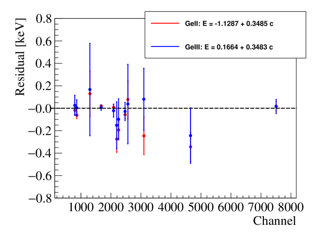
Figure 2: Fit residuals (defined as $E_{i}-E(\mu_{i})$) of a typical energy scale fit for GeII ($\chi^{2}=31.6$, ndf=10) in red and GeIII ($\chi^{2}=2.5$, ndf=10) in blue. Note that the error bars for some data points are too small to be seen. Low-event rate ²²⁸Th source data are shown. (Colors online)

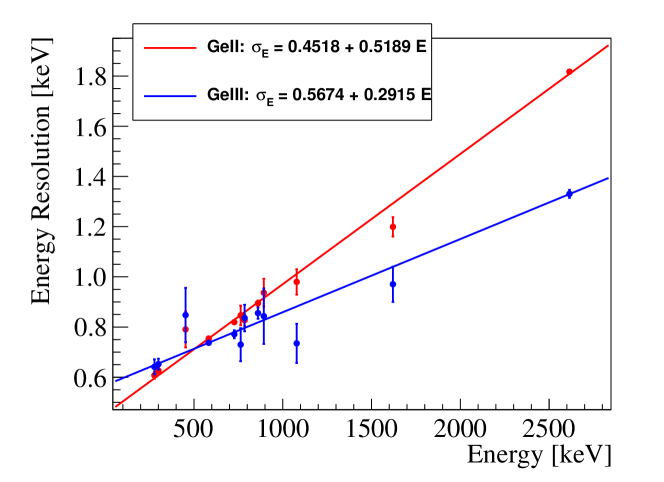
Figure 3: A typical energy resolution fit for GeII ($\chi^{2}=17.1$, ndf=10) in red and GeIII ($\chi^{2}=10.9$, ndf=10) in blue. Note that the error bars for some data points are too small to be seen. Low-event rate ²²⁸Th source data are shown. (Colors online)

3 Implementation in GEANT4

3.1 Geometry

All internal parts of GeII and GeIII and their endcaps are implemented in GEANT4 with boolean solids. The coded geometries are based on detailed technical information provided by the detector manufacturer for this purpose. Both the copper and the lead shieldings are implemented. The muon veto system, however, is not included as the scope of this work was, thus far, limited to the determination of counting efficiencies. A quantitative description of the detector backgrounds would require the modeling of the muon veto system. Figure 4 shows the GEANT4 renderings of GeII and GeIII.

3.2 Readout

For each simulated nuclear decay, all energy deposits in the active part of the germanium crystal are summed. To simulate the energy resolution of the actual detectors, the total energy is folded with a Gaussian resolution function with the following energy dependence:

$$E^{\prime}=E+\eta\cdot\sigma(E)$$ (6)

where $E$ is the total energy, $E^{\prime}$ is the smeared total energy, $\eta$ is a standard Gaussian random variable, and $\sigma(E)$ is the energy resolution of the actual detectors at $E$, as determined by calibration with radioactive sources.

The smeared total energy is mapped to the corresponding ADC channel ($C$) using the inverse of the energy calibration, mentioned above. Table 2 shows the parameters used in the simulation model for this purpose. This produces an uncalibrated energy spectrum similar to that delivered by the detector. This way, the same calibration and analysis procedure for actual data, as described in Section 2, can be applied to the simulated spectrum with minimal modification.

3.3 Coincident gammas

Coincident gammas are properly simulated by GEANT4 if the primary objects are the decaying nuclides as opposed to photons. In contrast, accidental coincidence of gamma rays originating from different nuclides are not considered by the simulation.

In practice, both kinds of coincidence have little effect in determining the detection efficiency.

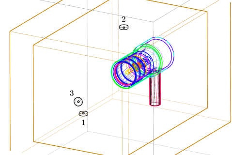
(a) GeII
 

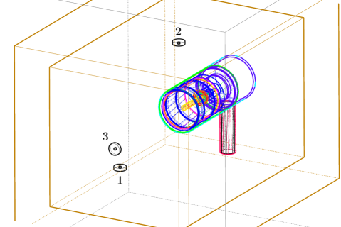
(b) GeIII

Figure 4: GEANT4 renderings of GeII (above) and GeIII (below). Also indicated on the renderings are the source positions labeled 1, 2 and 3. Positions 1 and 2 are flush with the detector front face. Position 1 is on the lower left edge of the chamber, while Position 2 is located under the ceiling of the chamber, above the central axis. Position 3 is located right inside the chamber door, on the central axis of the detector.

3.4 Dead layer tuning

Germanium crystals in p-type HPGe detectors typically have a “dead layer” on their outer surface that is insensitive to particle interactions. For GeII and GeIII, the nominal thicknesses of the dead layers, as specified by the manufacturer, are 0.9 mm and 0.7 mm, respectively. However, the thickness of the dead layer can change over time [2]. Hence, an estimation of the dead layer thickness needs to be made in order to appropriately model it in the simulation, especially at low energies (e.g. the modeling of ²¹⁰Pb decays).

To decide if the thickness of the dead layer needed to be tuned, the detection efficiencies of GeII and GeIII were measured and compared with those calculated by the simulation assuming nominal dead layer thicknesses. For the measurement, 4 button sources, ²²⁸Th, ¹³³Ba, ⁶⁰Co, and ⁵⁷Co, were placed in turn at Position 1 (as indicated in Figure 4). The results are shown in Figures 5(a) and 6 for GeII and GeIII, respectively.

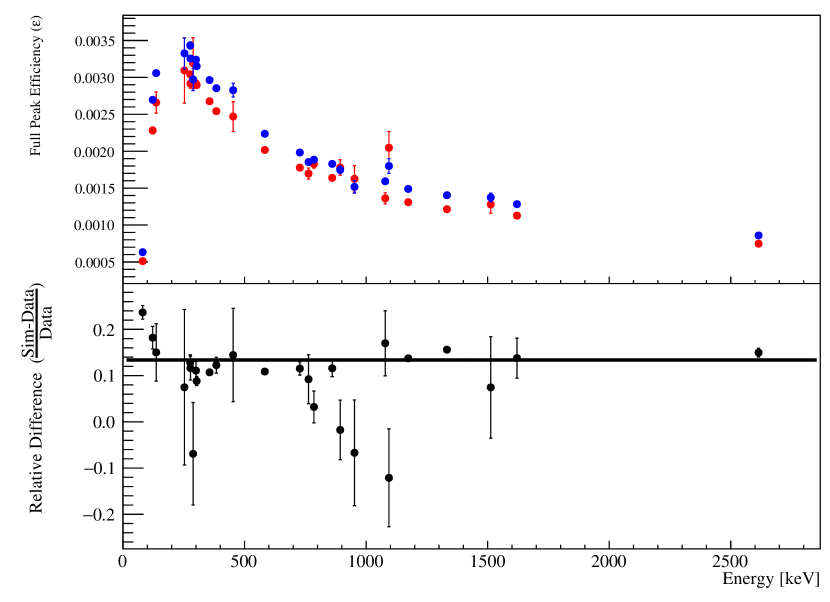
(a) Before dead layer tuning

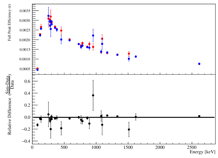
(b) After dead layer tuning

Figure 5: Relative difference in full absorption peak efficiency between simulation (blue) and data (red) for GeII with the source placed at Position 1 as in Figure 4(a). (Colors online)

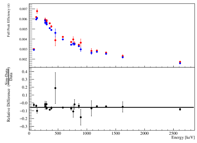
Figure 6: Relative difference in full absorption peak efficiency between simulation (blue) and data (red) for GeIII with the source placed at Position 1 as in Figure 4(b). (Colors online)

For GeIII, the simulation and the measurement show relatively small discrepancy ($<$10%). However, for GeII, the calculated efficiency is systematically higher than the measured value. There are two possible causes, both of which may contribute:

1. The actual dead layer thickness is larger than the nominal value. This causes additional attenuation to the gamma rays whose effect depends on the gamma energy.

2. The geometry in the simulation does not accurately reflect the actual geometry. In other words, the geometrical acceptance of the Ge crystal in the simulation differs from reality. This effect is largely independent of the gamma energy.

Cause (2) was indeed possible since the Ge detector and the cryostat, as one rigid body, can rotate around the penetration through the copper and the lead shielding. The Ge detector can therefore be accidentally nudged sideways by several millimeters during sample placement or LN₂ filling. The placement of the door can also affect the location of the source at position 3. Therefore, even though the source positions are defined as fixed points in the chamber , it is possible that the actual geometry (which can change slightly from run to run) differs from that in simulation which is static. This is sufficient to cause percent-level differences in detection efficiency. However, this is not intrinsic to the detector, and can be corrected for by aligning the detector before sample placement or by attaching the sample onto the end cap.

To eliminate the effect of geometrical differences and to focus only on the dead layer thickness, a loss function ${L}$ based on the mean squared error of the ratio of the measured and expected efficiencies is defined as follows:

$$\begin{cases}\rho_{i}(t_{+})=\displaystyle\frac{\varepsilon_{i}}{\varepsilon(E_{i})\cdot e^{-\mu(E_{i})\cdot t_{+}}}\\ {L}(t_{+})=\displaystyle\frac{1}{N_{\gamma}}\displaystyle\sum_{i=1}\rho_{i}^{2}(t_{+})-\left[\frac{1}{N_{\gamma}}\displaystyle\sum_{i=1}\rho_{i}(t_{+})\right]^{2}\end{cases}$$ (7)

where $t_{+}$ is the additional dead layer thickness beyond the nominal value, $E_{i}$ is the energy of the $i$th gamma peak out of a total of $N_{\gamma}$, $\varepsilon_{i}$ is the detection efficiency of the $i$th gamma peak as measured, $\varepsilon(E_{i})$ is the detection efficiency of the $i$th gamma peak calculated by simulation, $\mu(E_{i})$ denotes the attenuation coefficient for a photon with energy $E_{i}$ from the NIST XCOM database [3]. The optimal $t_{+}$ is the one that minimizes ${L}(t_{+})$. Notice that a difference in geometrical acceptance would manifest as an energy-independent pre-factor in $\rho_{i}(t_{+})$, (and hence in $L(t_{+})$) which has no effect on the value of the optimal $t_{+}$.

The detection efficiency of GeII was measured with 5 button sources: ¹³³Ba, ¹⁰⁹Cd, ⁵⁷Co, ⁵⁴Mn, and ²²Na placed in turn at Position 1. The measured and the simulated detection efficiency values were put into Equation 7. Figure 7 shows ${L}(t_{+})$ as $t_{+}$ is tuned in 10 $\mu$m steps up to 1 mm. ${L}(t_{+})$ reaches a minimum when $t_{+}=0.52$ mm. The dead layer thickness in the GEANT4 model of GeII was therefore adjusted from 0.9 mm to 1.42 mm. No adjustments were made to the dead layer of GeIII. Figure 8 shows the efficiency curves for GeII before and after dead layer tuning, along with the efficiency values measured with the five button sources.

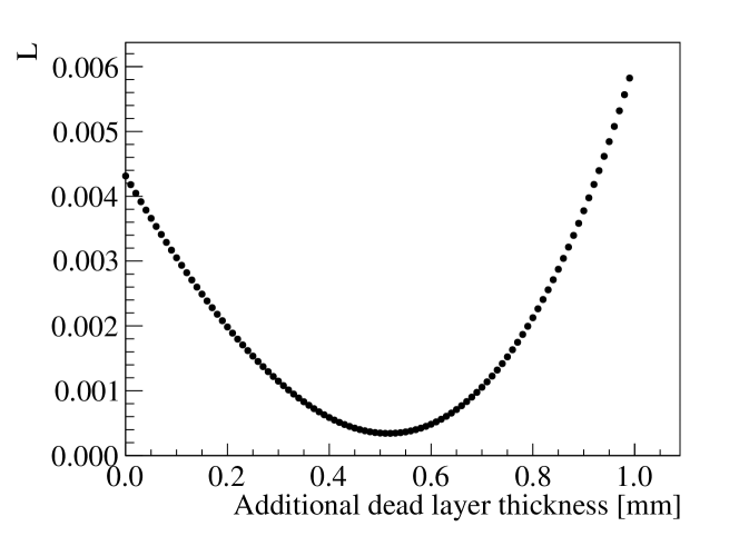
Figure 7: $L$ as a function of additional dead layer thickness on top of the nominal value. It reaches a minimum at 0.52 mm.

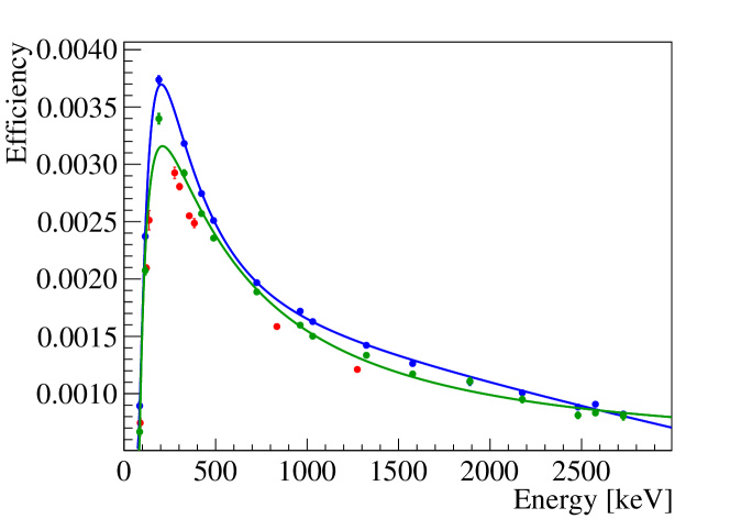
Figure 8: This figure shows the effect of dead layer tuning for GeII. The data points in red are the detection efficiencies measured with 5 button sources. The data points in blue are the detection efficiencies calculated with the simulation model before dead layer tuning, and the curve in blue is the fit. The data points and the curve in green are the same for after. (Colors online)

	Button Source	Button Source	Button Source	Source cocktail
	Position 1	Position 2	Position 3	in a bottle
GeII (before tuning)	$13.4\pm 0.2$	$12.1\pm 0.2$	$3.7\pm 0.3$	-
GeII (after tuning)	$-0.5\pm 0.3$	$3.0\pm 0.3$	$-3.0\pm 0.5$	$11.4\pm 0.3$
GeIII	$-5.7\pm 0.3$	$0.7\pm 0.3$	$-3.4\pm 0.4$	$8.6\pm 0.2$

Table 3: Percentage differences between measured and simulated detection efficiencies for the button sources and the source cocktail in GeII and GeIII, calculated as described in Section 4.1. Note that Position 1 was used to tune GeII’s dead layer thickness.

4 Validation

To ensure the model is robust against a change in sample location, sample geometry, and gamma energy, four sets of validations have been performed:

• Button sources located at different positions. This is to validate the performance of the model against a change in solid angle.

• A source cocktail in a bottle. This is to validate that the model properly handles extended sources in addition to point sources.

• Lead(II) nitrate [Pb(NO₃)₂] solution, for low photon energies.

• Silica (SiO₂) spiked with ²³⁸U, ²³²Th and ⁴⁰K. This serves as an independent cross-check of the efficiency correction, compared to other germanium detectors operated outside UA.

4.1 Position dependence: Button sources at different positions

The ²²⁸Th, ¹³³Ba, ⁶⁰Co, and ⁵⁷Co button sources, the same ones used for dead layer check, were placed at locations 2 and 3, as indicated in Figure 4. The efficiencies were calculated as described in Section 2 and compared with the simulation. The agreement between simulation and measurement was quantified by the average relative difference between simulation and measurement, weighted by the inverse square of the uncertainty for each peak. These averages, as seen in Table 3, indicate that simulated and measured efficiencies agree to within $\sim$5%.

4.2 Extended source: Source cocktail in a bottle

To check the performance of the model for a source with an extended shape, a “source cocktail” (with its contents listed in Table 4) was created as follows:

1. An empty, clean 125 mL polyethylene (PE) bottle was filled with 4M HCl to about half full.

2. A total of $420.2\pm 0.8$ $\mu$L of a calibrated Eckert & Ziegler source solution, which contained ¹⁰⁹Cd, ¹³⁹Ce, ⁵⁷Co, ⁶⁰Co, ¹³⁷Cs, ¹¹³Sn and ⁸⁸Y dissolved in HCl, was transferred to the PE bottle. The transfer was performed in 10 iterations with a 50 $\mu$L syringe.

3. The PE bottle was topped off with 4M HCl to the intended fill level.

Nuclide	$E_{\gamma}$	$\gamma$ branching	Half-life	$\gamma$ emissivity [$\gamma$/s]
	[keV]	fraction	[d]	on Nov 22, 2013
57Co	14.4	0.0916	271.74	2.161
109Cd	88.0	0.0364	461.4	86.12
57Co	122.1	0.8560	271.8	20.19
57Co	136.47	0.1068	271.8	2.519
139Ce	165.9	0.8000	137.6	4.029
113Sn	255.1	0.0211	115.1	0.0739
113Sn	391.7	0.6497	115.1	2.599
137Cs	661.7	0.8510	10980	176.3
88Y	898.0	0.937	106.6	4.288
60Co	1173.2	0.9985	1925.28	260.3
60Co	1332.5	0.9998	1925.28	260.3
88Y	1836.1	0.992	106.6	4.539

Table 4: Listing of gamma radiation emitted by the “source cocktail” and their emissivities at the data taking date (Nov 22, 2013). Gamma energies, branching fraction, and half-lives are taken from [4]. The calculations were made assuming that the radio nuclides in the source solution were homogeneously distributed throught the solution and that the residue left in the syringe after the transfers was negligibly small.

The source cocktail was counted in GeII and GeIII separately in the geometry shown in Figure 9. Figure 10 shows a comparison between the measured and simulated spectra for GeIII. The full absorption peak efficiencies for GeII and GeIII are shown in Figures 11 and 12, respectively. The differences between the measurement and simulation, calculated the same way as described in Section 4.1, are (11.4 $\pm$ 0.3)% and (8.6 $\pm$ 0.2)% for GeII and GeIII respectively (also tabulated in Table 3.)

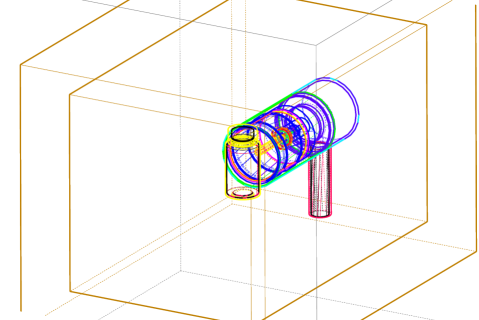
Figure 9: Geometry for the source cocktail and the ²¹⁰Pb solution. The Geant4 implementation of the PE bottle geometry was based on measurements with a caliper.

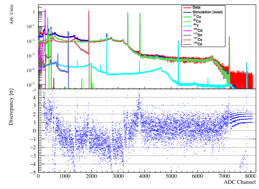
Figure 10: The upper portion shows a comparison between (blue) simulated and (red) measured spectra for the “source cocktail”. The simulated spectra of the individual isotopes are in various colors indicated in the legend. The lower portion shows the discrepancy between measurement and simulation, defined as $\frac{x_{i}-y_{i}}{\sqrt{\sigma_{x_{i}}^{2}+\sigma_{y_{i}}^{2}}}$ where $x_{i}$ and $y_{i}$ are the contents of the $i$th bin of the measurement and the simulation respectively, and $\sigma_{x_{i}}$ and $\sigma_{y_{i}}$ are their respective statistical errors. (Colors online)

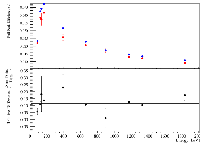
Figure 11: Relative difference in full absorption peak efficiency between simulation (blue) and data (red) for the source cocktail in GeII. (Colors online)

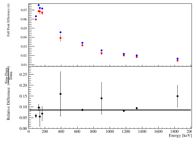
Figure 12: Relative difference in full absorption peak efficiency between simulation (blue) and data (red) for the source cocktail in GeIII. (Colors online)

4.3 Low energy region: ²¹⁰Pb(NO₃)₂ solutions

The performance of the model for GeIII at low energy ($E_{\gamma}=46.54$ keV) was validated with three ²¹⁰Pb sources prepared by diluting a standard stock solution of lead-210 nitrate (²¹⁰Pb(NO₃)₂) from Eckert & Ziegler with BDH ARISTAR PLUS®  nitric acid (HNO₃) for trace metal analysis from VWR. This validation was not performed for GeII, which is equipped with a copper end cap, as its detection efficiency of a photon with such a low energy was expected to be too low to be useful.

The sources were prepared as follows:

1. 54.1 mL of 70% HNO₃ was diluted to 1M with 795.8 g of deionized water.

2. 5 $\mu$L of the ²¹⁰Pb(NO₃)₂ solution was added to 410.4 g of the 1M HNO₃.

3. The diluted ²¹⁰Pb(NO₃)₂ solution was filled into three 125 mL PE bottles, the same kind as the “source cocktail”.

The bottles were labeled A1, B1 and C1. Given that the specific activity of the stock solution was 3.72 $\pm$ 0.15 kBq/g on April 1, 2017 (derived from the calibration certificate supplied by the manufacturer), the specific activity of the diluted sample solutions was calculated to be 46.8 $\pm$ 2.1 Bq/kg on the same day.

The samples were counted in GeIII in the geometry shown in Figure 9. The results obtained in this test (tabulated in Table 5) are consistent with the expected specific activity to within 7% or about 0.7 standard deviations.

Sample	Count rate	Net sample	Measured specific
label	[counts/day]	mass [g]	activity [Bq/kg]
A1	309.5 $\pm$ 14.4	133.1	48.4 $\pm$ 7.7
B1	317.0 $\pm$ 14.6	130.3	50.7 $\pm$ 8.0
C1	323.7 $\pm$ 13.9	130.9	51.5 $\pm$ 8.1
Mean			50.2 $\pm$ 4.6

Table 5: Data-derived specific activity of ²¹⁰Pb in the three tested sample solutions using measured data and efficiency parametrization from simulation. The expectation value for this specific activity is $46.8\pm 2.1$ Bq/kg (statistical uncertainty only).

4.4 Cross-check among Ge analysis teams: Spiked silica samples

This cross-check was performed as a validation among the three Ge analysis teams within the nEXO collaboration, who operate the following detectors: 1) GeII and GeIII at the University of Alabama, 2) the detector at Vue-des-Alpes (VdA) operated by the University of Bern [5], and 3) the PGT detector at SNOLAB. In addition to the different physical locations of the Ge detectors, there are also differences in the analysis methods among the teams as listed in Table 6. For example, the energy scale is linear for GeIII and VdA, but quadratic at SNOLAB. Also, the detection efficiency is modeled as Equation 5 for GeIII, but as the following equation for SNOLAB.

$$\varepsilon(E)=10^{\nu_{1}+\nu_{2}\cdot E+\nu_{3}\cdot E^{-1}+\nu_{4}\cdot E^{-2}+\nu_{5}\cdot E^{-3}+\nu_{6}\cdot E^{-4}},$$ (8)

where $\nu_{1}$, $\nu_{2}$, … ,$\nu_{6}$ are free varying parameters. The VdA team does not use any analytical model, instead efficiencies between simulated energy points are linearly interpolated. This exercise is to ensure that the Ge analyses done at various institutes are consistent with each other. As such, it serves as an additional consistency test for the efficiency correction derived from the numerical detector model discussed in the paper.

Analysis Team	GeIII	VdA	SNOLAB
Data taking
Typical length of runs	24 hours	24 to 72 hours	5 or 10 minutes
Radon mitigation	First 24 hours of data is discarded.	First 24 hours of data is discarded.	Sample preconditioned with Radon-poor air
Energy scale calibration
Model	Linear function	Linear function	Quadratic function
Continuum background subtraction
Method	Count rates are obtained by fitting the peak and the continuum at the same time with a Gaussian + linear model. The count rate is the integral of the Gaussian divided by the measurement time.	Count rates are obtained by integrating over a width of 2 FWHM around the peak. The continuum is linearly extrapolated and then subtracted from the peak integral.	Count rates are obtained by integrating over a region of a certain width around the peak. The continuum is estimated by integrating over a region of the same width to left and another to the right of the peak. The average of the two is subtracted from the peak integral.
Detection efficiency calculation
Simulation tool	GEANT4	GEANT4	GEANT4
$\varepsilon(E)$	Efficiencies at various energies are calculated by simulation. They are then fitted with Equation 5.	Efficiencies at various energies are calculated by simulation. Efficiencies at intermediate energies are linearly interpolated as needed.	Efficiencies at various energies are calculated by simulation. They are then fitted with Equation 8.

Table 6: Comparison of the standard data taking and analysis procedure among the three Ge analysis teams.

For this check, three samples were prepared at SNOLAB by adding measured amounts of three standard reference materials, purchased from the International Atomic Energy Agency (IAEA): RGU-1 (containing uranium), RGTh-1 (containing thorium), and RGK-1 (containing potassium), to silica (Fisher Scientific catalog number S-153, lot number 111211). The actual spike amounts were blinded from the analysis teams.

The samples were prepared in the following way [6]:

1. Three 2 L PE bottles were filled with about 1460 grams of inactive silica at SNOLAB.

2. About 60 grams of RGU-1, RGTh-1 and RGK-1 were respectively added to individual PE bottles with silica.

3. Each of the PE bottles was mixed for 24 hours to ensure thorough mixing.

4. From each of the PE bottles, 4 grams of the mixture was transferred to a 3 mL Teflon bottle. The three Teflon bottles were labeled U2, T2, and K2 corresponding to the mixtures containing RGU-1, RGTh-1 and RGK-1 respectively.

The samples were then counted and analyzed using the GeIII, VdA, and SNOLAB detectors. The results from the three analysis teams are consistent with each other as can be seen in Table 7.

Sample	Isotope	GeIII	VdA	SNOLAB
U2	238U	$180\pm 2$	$164\pm 2$	$180\pm 5$
T2	232Th	$115\pm 2$	$108\pm 1$	$116\pm 4$
K2	40K	$341\pm 10$	$292\pm 14$	$377\pm 30$

Table 7: Specific activities in Bq/kg of U2, T2 and K2 as measured by the three analysis teams. The errors are statistical only. Systematic errors are expected to be $\sim$10% for all three teams.

5 Conclusion

The GEANT4 models for GeII and GeIII have been validated in the energy range and the geometrical configurations relevant to typical radioassay measurements. By rounding up the largest differences in measured and simulated detection efficiencies for the button sources and the source cocktail shown in Table 3, the systematic uncertainties of the models for GeII and GeIII are conservatively estimated to be $\sim$12% and $\sim$9% respectively.

References

- [1] S. Agostinelli et al., GEANT4 – a simulation toolkit, Nucl. Instr. and Methods A506, 3, 250-303 (2003)
- [2] G. F. Knoll, Radiation Detection and Measurement, 3rd Edition. (2000)
- [3] M. J. Berger et al., XCOM: Photon Cross Section Database (version 1.5), http://physics.nist.gov/xcom, accessed on October 30, 2018.
- [4] A. A. Sonzogni, NuDat 2.0: Nuclear Structure and Decay Data on the Internet, AIP Conference Proceedings 769, 574 (2005). https://www.nndc.bnl.gov/nudat2
- [5] P. Weber, B. A. Hofmann, T. Tolba, and J.-L. Vuilleumier, A gamma-ray spectroscopy survey of Omani meteorites, Meteoritics & Planetary Science 52, Nr 6, 1017–1029 (2017)
- [6] B. Cleveland, Preparation and Properties of SNOLAB Radiological Sources SRS-12-004 SRS-12-005 SRS-12-006 – Calibration Sources for Ge Well Detector, SNOLAB document, dated 28 March 2013.