Ordered Line Integral Methods for Solving the Eikonal Equation

Abstract

We present a family of fast and accurate Dijkstra-like solvers for the eikonal equation and factored eikonal equation which compute solutions on a regular grid by solving local variational minimization problems. Our methods converge linearly but compute significantly more accurate solutions than competing first order methods. In 3D, we present two different families of algorithms which significantly reduce the number of FLOPs needed to obtain an accurate solution to the eikonal equation. One method employs a fast search using local characteristic directions to prune unnecessary updates, and the other uses the theory of constrained optimization to achieve the same end. The proposed solvers are more efficient than the standard fast marching method in terms of the relationship between error and CPU time. We also modify our method for use with the additively factored eikonal equation, which can be solved locally around point sources to maintain linear convergence. We conduct extensive numerical simulations and provide theoretical justification for our approach. A library that implements the proposed solvers is available on GitHub.

1 Introduction

We develop fast, memory efficient, and accurate solvers for the eikonal equation, a nonlinear hyperbolic PDE encountered in high-frequency wave propagation engquist2003computational and the modeling of a wide variety of problems in computational and applied science sethian1999level , such as photorealistic rendering ihrke2007eikonal , constructing signed distance functions in the level set method osher2006level , solving the shape from shading problem kimmel2001optimal ; prados2006shape ; durou2008numerical , traveltime computations in numerical modeling of seismic wave propagation sethian19993 ; popovici20023 ; kim20023 ; van1991upwind ; vidale1990finite , and others. We are motivated primarily by problems in high-frequency acoustics prislan2016ray , which are key to enabling a higher degree of verisimilitude in virtual reality simulations (see raghuvanshi2014parametric ; raghuvanshi2018parametric for a cutting-edge time-domain approach which is useful up to moderate frequencies). Current approaches to acoustics simulations rely on methods whose complexity depends on the highest frequency of the sound being simulated. For moderately high-frequency wave propagation problems, the eikonal equation comes about as the first term in an asymptotic WKB expansion of the Helmholtz equation and corresponds to the first arrival time of rays propagating under geometric optics, although approaches for computing multiple arrivals exist fomel2002fast .

In this work, we develop direct solvers for the eikonal equation which are fast and accurate, particularly in 3D. We develop a family of algorithms which approach the problem of efficiently computing updates in 3D in different ways. This family of algorithms is analyzed and extensive numerical studies are carried out. Our algorithms are semi-Lagrangian, using information about local characteristics to reduce the work necessary to get an accurate result. They are competitive with existing direct solvers for the eikonal equation and generalize to higher dimensions and related equations, such as the static Hamilton-Jacobi equation. In fact, this research was done in tandem with research on the ordered line integral methods for the quasipotential of nongradient stochastic differential equations (SDEs) dahiya2017ordered ; dahiya2018ordered ; yang2019computing . Due to the relative simplicity of the eikonal equation, the algorithms presented here are more amenable to analysis, allowing us to obtain theoretical results that justify our experimental findings.

1.1 Results

Figure 1: The family of Dijkstra-like solvers designed and studied in this work. We refer to these as ordered line integral methods (OLIMs). There are three ways of parametrizing the family: by selecting an update algorithm, by selecting a quadrature rule, and by (in the case of the top-down update algorithm, by selecting a neighborhood size. Sections in the text that explain these choices in detail are indicated. A shorthand notation for referring to each parametrized algorithms is listed for each algorithm that is involved in numerical tests (e.g., olim3d_mp0).

Different numerical methods have been proposed for the solution of the eikonal equation; generally, there are direct solvers and iterative solvers. The most popular direct solvers are based on Dijkstra’s algorithm (“Dijkstra-like” solvers) tsitsiklis1995efficient ; sethian1996fast , and the most popular iterative method is the fast sweeping method tsai2003fast ; zhao2005fast . In this work, we develop a family of Dijkstra-like solvers for the eikonal equation in 2D and 3D, similar to the fast marching method (FMM) or ordered upwind methods (OUMs) sethian1996fast ; sethian2003ordered . In constrast to the FMM and OUMs that use finite difference schemes, our solvers come about by discretizing and minimizing the action functional for the eikonal equation (see section A). The proposed family of algorithms is parameterized by a choice of update algorithm (bottom-up or top-down), quadrature rule (a righthand rule (rhr), a simplified midpoint rule (mp0), and a midpoint rule (mp1)), and, in the case of bottom-up, a neighborhood size (6, 18, or 26 points in 3D). See figure 1.

Our bottom-up and top-down update algorithms represent two separate approaches to minimizing the number of triangle and tetrahedron updates that need to be done in 3D, while the quadrature rules represent a trade-off between speed and accuracy of the solver. The simplified midpoint rule (mp0) is a sweet spot that requires extra theoretical justification, which we provide. Overall, our goal is to explore the relevant algorithm design trade-offs in 3D and find which solver performs best. Our conclusion is that, in 3D, olim3d_mp0 is the best overall, and our results are oriented towards supporting this claim.

Additionally, we modify our algorithms to solve the additively factored eikonal equation luo2012fast : to enhance accuracy, we solve the locally factored eikonal equation near point sources, which recovers the global $O(h)$ error convergence expected from a first-order method, where $h>0$ is the uniform spacing between grid points. This fixes the degraded $O(h\log h^{-1})$ convergence often associated with point source eikonal problems qi2018corner (see zhao2005fast for a proof of this error bound).

Our main results follow:

• For 3D problems, we develop two separate update algorithms: a bottom-up (olim3d) algorithm, and a top-down algorithm (olimK, where K $=6,18,26$ is the size of neighborhood used). Each algorithm locally updates a grid point by performing a minimal number of triangle or tetrahedron updates. Depending on the quadrature rule, each update is calculated by solving a system of nonlinear equations either directly (rhr and mp0) or iteratively (mp1).

• We prove theorems relating our quadrature rules, rigorously justifying the mp0 rule. These results support our case that it is superior to the mp1 rule. We note that this work was done in tandem with research on ordered line integral methods for computing the quasipotential 3D for nongradient SDEs dahiya2017ordered ; yang2019computing ; dahiya2018ordered . Unlike the quasipotential, the eikonal equation is simple enough to allow us to analyze and justify our algorithms. We are also able to obtain simpler solution methods and established performance guarantees.

• We conduct numerical experiments on test problems with analytic solutions. The test problems include point source problems for different slowness (index of refraction) functions, and multiple point source problems with a linear speed function. All of these have analytical solutions, which we use as a ground truth. We also test our

• We perform tests involving the Marmousi model in 2D and 3D. We demonstrate that the improved directional coverage of olim26 and olim3d leads to a gain in accuracy.

• We show that a significant improvement in accuracy is gained over the equivalent of the standard fast marching method in 3D, olim6_rhr. Only a modest slowdown is incurred using our general framework, indicating that our approach is competitive. See figure 2 to see the improvement of olim3d_mp0 over olim6_rhr, and see section 5 for more details.

• We use Valgrind nethercote2007valgrind to profile our implementation. Our results indicate that the time spent sorting the heap used to order nodes on the front is negligible for all practical problem sizes. Since our solvers otherwise run in $O(N^{n})$ time, where $n$ is the dimension of the domain, we suggest that the $O(N^{n}\log N)$ cost of the algorithm is pessimistic. Memory access patterns play a much more significant role in scaling.

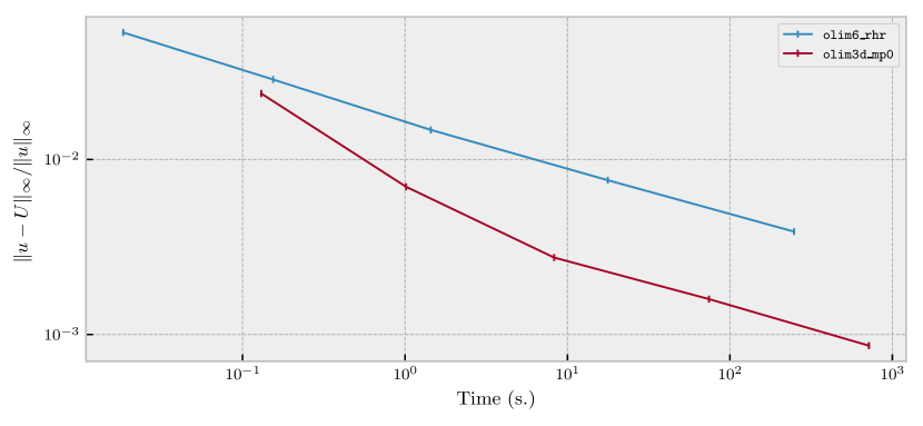
Figure 2: Comparing the relative $\ell_{\infty}$ errors of olim3d_mp0 and olim6_rhr. For the multiple point source problem in section 5.3 with the domain $\Omega=[0,1]^{3}$ discretized in each direction into $N=2^{p}+1$ (where $p=5,\ldots,9$), the total number of grid points is $N^{3}$.

1.2 Accessing our library

Our implementation is in C++ stroustrup2013c++ . A link to a project website on GitHub can be accessed from S. Potter’s website sfp-umiacs-homepage . The GitHub site includes instructions for downloading and running basic examples libolim-github . The code used to generate plots in this paper is also available with instructions libolim-github-plotting .

2 Background

In this section we provide a brief overview of the eikonal equation and its numerical solution on a regular grid and sketch a generic Dijkstra-like algorithm which we will refer to throughout the paper to organize our results.

2.1 The eikonal equation

With $n\geq 2$, and given a domain $\Omega\in\mathbb{R}^{n}$, the eikonal equation is:

$$\left\|\nabla u(x)\right\|=s(x),\qquad x\in\Omega,$$ (1)

where $\|\cdot\|$ denotes the $\ell_{2}$ norm unless otherwise stated, and $s:\Omega\to(0,\infty)$ is a fixed, positive slowness function, which forms part of the data. We solve for $u:\Omega\to\mathbb{R}_{+}$. The boundary data is provided on a subset $D\subset\Omega$ where $u$ has been fixed; i.e., $\left.u\right|_{D}=g$ for some $g:D\to\mathbb{R}_{+}$. As an example, if $s\equiv 1$ and $g\equiv 0$, then the solution of eq. 1 is:

$$u(x)=d(x,D)=\min_{y\in D}\left\|x-y\right\|.$$ (2)

That is, $u$ is the distance to $D$ at each point in $\Omega$.

To numerically solve eq. 1, first let $\mathcal{G}=\{p_{i}\}\subseteq\Omega$ be the set or grid of nodes where we would like to approximate the true solution $u$ with a numerical solution $U:\mathcal{G}\to\mathbb{R}_{+}$. Additionally, for each node $p\in\mathcal{G}$, define a set of neighbors, $\texttt{nb}(p)\subseteq\mathcal{G}\backslash\left\{p\right\}$. Typically—for the FMM, for instance—$\mathcal{G}$ is taken to be a subset of a lattice in $\mathbb{R}^{n}$ and $\texttt{nb}(p)$ to be each node’s $2n$ nearest neighbors. We also define the set of boundary nodes, $\texttt{bd}\subseteq\mathcal{G}$. It may happen that the set bd and $D$ do not coincide (e.g., $D$ could be a curve which does not intersect any points in $\mathcal{G}$); to reconcile this difference, the initial value of $U(p)$ for each $p\in\texttt{bd}$ must take $g=\left.u\right|_{D}$ into account in the best way possible. This problem has been approached in different ways, and is not the focus of the present work chopp2001some .

Throughout, we make several simplifying assumptions.

• All boundary nodes coincide with grid points: $\texttt{bd}=D\subseteq\mathcal{G}$.

• The grid $\mathcal{G}$ is a regular, uniform grid (a subset of a regular, uniform square lattice in 2D or cubic lattice in 3D). We denote grid nodes by $x\in\mathcal{G}$.

• When numerically computing a new value at a grid point $\hat{x}\in\mathcal{G}$, we transform the neighborhood to the origin and scale the vertices so that they have integer values. The transformed update node is labeled $\hat{p}$. See section 3.1 for a detailed explanation.

2.2 Dijkstra-like algorithms

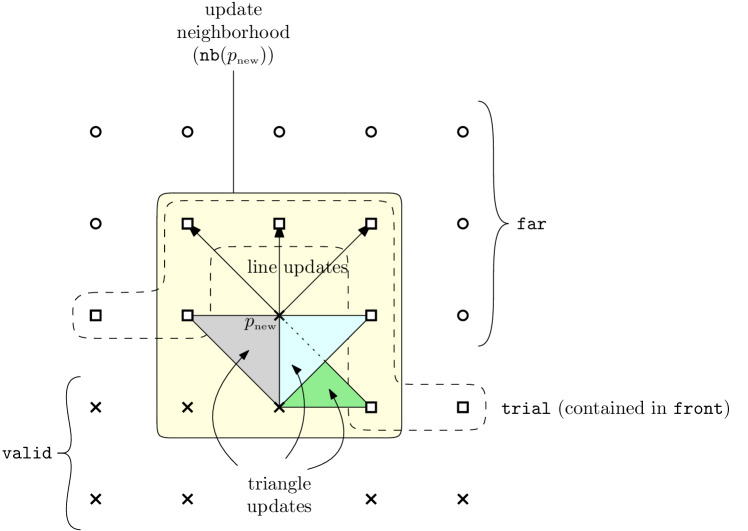
Figure 3: An overview of a Dijkstra-like algorithm for solving the eikonal equation (eq. 1) in 2D. See alg. 1 for details. Nodes are labeled by state so that $\circ=\mathtt{far}$, $\square=\mathtt{trial}$, and $\times=\mathtt{valid}$. In this diagram, the node $p_{\operatorname{new}}$ has been removed from front and had its state set to valid. All far nodes in $\texttt{nb}(p_{\operatorname{new}})$ are set to trial, and then all trial nodes in $\texttt{nb}(p_{\operatorname{new}})$ are updated. The updates are depicted: there are three line updates and three triangles, since it is only necessary to perform updates that involve $p_{\operatorname{new}}$. The OLIM shown here is olim8. In 3D, there would also be tetrahedron updates.

If we order nodes in $\mathcal{G}$ so that new solution values are only computed using upwind nodes, the eikonal equation can be solved directly; i.e., without the use of an iterative solver. This is done using a continuous version of Dijkstra’s algorithm for finding shortest paths in a network. Other algorithms which solve similar network flow problems can also be used, but have different complexity guarantees chacon2012fast . In particular, Dijkstra’s algorithm is a type of label-setting method for finding shortest paths in a network; there are also label-correcting methods bertsekas1998network .

Using Dijkstra’s algorithm to solve a “continuous shortest path” problem has been discovered in several contexts. The earliest such development is a theoretical result in computational geometry due to Mitchell, Mount, and Papadimitriou, who used this idea to compute exact polyhedral shortest paths (“discrete geodesics”) on triangulated surfaces mitchell1987discrete . This was followed by Tsitsiklis who developed a first-order semi-Lagrangian method for solving isotropic optimal control problems on a uniform grid tsitsiklis1995efficient . Finally, the fast marching method, which uses a first-order upwind finite difference scheme was developed by Sethian to model isotropic front propagation sethian1996fast . Many variations of these methods have since been developed sethian2003ordered ; kao2008legendre . Our own development resembles Tsitsisklis’s, but extends it past its original formulation. In particular, Tsitsiklis considers what we call olim8_rhr and olim26_rhr, and does not treat the 3D case in depth. We generalize this approach, considering higher accuracy quadrature rules (mp0 and mp1) and algorithms which make 3D solvers fast (our bottom-up and top-down algorithms). We also note that Bornemann and Rasch have investigated the local variational approach (à la Tsitsiklis), and have present detailed theoretical results—their approach is complementary to our own, but has a much different emphasis bornemann2006finite .

To write down a generic Dijkstra-like algorithm, there are several pieces of information which need to be kept track of. A data structure called front tracks trial nodes while the solver runs (typically an array-based heap). For each node $p$, apart from the current value of $U(p)$, the most salient piece of information is its state, written $p$.state $\in\left\{\texttt{valid},\texttt{trial},\texttt{far}\right\}$. To fix ideas, consider the following high-level Dijkstra-like algorithm:

Algorithm 1 A generic Dijkstra-like algorithm for solving the eikonal equation.

1. For each $p\in\mathcal{G}$, set $p$.state $\leftarrow$ far and $U(p)\leftarrow\infty$.

2. For each $p\in\texttt{bd}$, set $p$.state $\leftarrow$ trial, and set $U(p)$ to a user-defined value.

3. While there are trial nodes left in $\mathcal{G}$:

   1. Let $p_{\operatorname{new}}$ be the trial node in front with the smallest value $U(p_{\operatorname{new}})$.

   2. Set $p_{\operatorname{new}}$.state $\leftarrow$ valid and remove $p_{\operatorname{new}}$ from front.

   3. For each $\hat{p}\in\texttt{nb}(p_{\operatorname{new}})$, set $\hat{p}$.state $\leftarrow$ trial if $\hat{p}$.state $=$ far.

   4. For each $\hat{p}\in\texttt{nb}(p_{\operatorname{new}})$ such that $\hat{p}$.state $=$ trial, update $\hat{U}=U(\hat{p})$ and merge $\hat{p}$ into front.

Specifying how item 3d is to be performed is the crux of developing a Dijkstra-like algorithm and is left intentionally vague here. This step involves indicating how nodes in $\texttt{nb}(\hat{p})$ are used to compute $\hat{U}$, and how they are organized into the front data structure. The FMM uses an upwind finite difference scheme where only valid nodes are used to compute $\hat{U}$, and where nodes on the front are sorted using an array-based heap implementing a priority queue sethian1996fast . As an example, Tsitsiklis’s algorithm combines nodes in valid into sets whose convex hulls approximate the surface of the expanding wavefront and then solves local functional minimization problems. The method presented here is more similar to Tsitsiklis’s algorithm (see figure 3). For specific details, a general reference should be consulted sethian1999level .

In addition to item 3d, algorithm 1 is generic in the following ways:

• As we mentioned before, there are different ways of initializing the boundary data bd if only off-grid boundary data is provided chopp2001some .

• How we keep track of the node with the smallest value is variable: most frequently, as in Dijkstra’s algorithm, a heap storing pointers to the nodes is used, leading to $O(N^{n}\log N)$ update operations overall, where $N^{n}$ is the number of nodes. In fact, there are $O(N^{n})$ variations using Dial’s algorithm (a bucketed version of Dijkstra’s algorithm), but these have not been used as extensively as Dijkstra-like algorithms tsitsiklis1995efficient ; kim2001calo ; yatziv2006n .

• The arrangement of the nodes into a grid or otherwise varies, as do the neighborhoods of each node. This affects the update procedure. A regular grid is simple to deal with, but Dijkstra-like methods have been extended to manifolds and unstructured meshes, where the situation is more involved kimmel1998computing ; sethian2000fast ; bronstein2008numerical .

Other problems can be solved using Dijkstra-like algorithms: the static Hamilton-Jacobi equation, an anisotropic generalization of the eikonal equation, can be solved using the ordered upwind method sethian2003ordered or other recently introduced methods mirebeau2014efficient ; mirebeau2014anisotropic . The quasipotential of a nongradient stochastic differential equation can also be computed using the ordered line integral method, although the considerations are more involved dahiya2017ordered ; dahiya2018ordered ; yang2019computing .

2.3 Fast sweeping methods

Another approach to solving a discretized version of eq. 1 is the fast sweeping method tsai2003fast ; zhao2005fast . Unlike Dijkstra-like methods, which are direct solvers, the fast sweeping method is an iterative solver using an upwind scheme and rotating sweep directions, which obtains $O(N^{n})$ complexity—however, the constant in this asymptotic estimate depends heavily on how frequently the characteristics change direction, and how complicated the geometry of the domain is. Fast sweeping methods have been extended to Hamilton-Jacobi equations tsai2003fast ; kao2008legendre , and hybrid methods combining the fast sweeping method with a Dijkstra-like method have been introduced recently chacon2012fast ; chacon2015parallel . Additionally, higher-order fast sweeping methods based on ENO and WENO schemes have been developed zhang2006high . Luo and Zhao also provide a detailed investigation of the convergence properties of fast sweeping methods for static convex Hamilton-Jacobi equations, but with a focus on the 2D case luo2016convergence .

3 Ordered line integral methods for the eikonal equation

The fast marching method sethian1996fast solves a discretized eikonal equation (eq. 1) in an upwind fashion. Throughout, we distinguish between the exact solution $u$ and the numerical solution $U$, where $\hat{U}$ will always denote the current value to be computed; likewise, any quantity with a hat (^) will denote a quantity evaluated at the node being updated. The ordered line integral method locally and approximately minimizes the minimum action integral of eq. 1:

$$\hat{u}=\min_{\alpha}\left\{u_{0}+\int_{\alpha}s(x)dl\right\},$$ (3)

where $\alpha$ is a ray parametrized by arc length, $\hat{x}$ is a target point, $\hat{u}=u(\hat{x})$, and $u_{0}=u(\alpha(0))$ (see section A for a derivation of eq. 3). By constrast, Lagrangian methods (i.e., raytracing methods) trace a bundle of rays from a common locus by integrating Hamilton’s equations for the eikonal equation for different initial conditions.

In this section, we describe how we discretize and minimize an approximation of eq. 3. As we mentioned in section 2.2, to compute $\hat{U}=U(\hat{p})$ in item 3d of algorithm 1, we need to approximately minimize several instances of an approximation to eq. 3; details of this procedure are discussed in section 4. In this section, we focus on a single instance of the discretized version of eq. 3. We present our notation, derive prelimary results, and describe the quadrature rules mp0, mp1, and rhr. We also show how the functional minimization problem can be solved exactly using a QR decomposition for the rhr and mp0 rules. Finally, we present theoretical results justifying our approach.

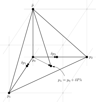
Figure 4: Overview of a tetrahedron update, showing the notation in section 3. Left: a point being updated, $\hat{p}$, which is identified with the origin, and three neighboring points $p_{0},p_{1}$, and $p_{2}$ that are assumed to be valid. The grid $\mathcal{G}$, which contains other points in the discretized domain, is sketched in light grey. The domain of the minimization problem eq. 14 is the convex hull of $p_{0},p_{1}$, and $p_{2}$. The path minimizing eq. 3 is assumed to be the line segment connecting $\hat{p}$ and $p_{\lambda}$. Not pictured is the newly valid point $p_{\operatorname{new}}$, although it is assumed that $p_{\operatorname{new}}$ equals one of $p_{0},p_{1}$, or $p_{2}$. Right: the same update tetrahedron, but this time with quantities related to the slowness function depicted.

3.1 Approximating the action functional

In this section we describe how we approximate eq. 3 and reformulate it as a constrained optimization problem which we solve to update the trial nodes surrounding a node $p_{\operatorname{new}}$ which has just become valid.

First, we assume that $\Omega\subseteq\mathbb{R}^{n}$, where $n=2,3$. The methods presented here work for general $n$. We refer to each update as a “simplex update”, since for a dimension $n$, we need to consider updates of dimensions $d$ where $0\leq d<n$. For $n=3$, we have line updates ($d=0$), triangle updates ($d=1$), and tetrahedron updates ($d=2$). So, $d$ refers to the dimension of the base of each simplex, which is the dimension of the domain of the optimization problem that we will formulate.

We assume that each update simplex is nondegenerate and that the convex hull of the update point $\hat{p}$ and $d+1$ points $p_{0},\ldots,p_{d}\in\texttt{nb}(\hat{p})$. Since we assume that our grid $\mathcal{G}$ is uniform and rectilinear, we scale and translate $\mathcal{G}$ so that $\hat{p}=0$ and $\|p_{i}\|_{\infty}=1$ for $i=0,\ldots,d$. Throughout the rest of the paper, we always shift the node $\hat{p}$ to the origin, as this simplifies our calculations.

Approximating the integration path with a straight line segment.

To approximately minimize eq. 3 we assume that the minimizing path is a straight line segment connecting $\hat{p}$ and a point in the convex hull of $\{p_{0},\ldots,p_{d}\}$, and numerically approximate the action over this integral path using quadrature. We discuss each part of this approximation in turn. First, some notation.

We parametrize the “base of the update simplex” (the convex hull of $p_{0},\ldots,p_{d}$) over the set:

$$\Delta^{d}=\left\{\lambda_{i}\geq 0\mbox{ for }i=1,\ldots,d\mbox{ and }\sum_{i=1}^{d}\lambda_{i}\leq 1\right\}.$$ (4)

If we let $\lambda_{0}=1-\sum_{i=1}^{d}\lambda_{i}$, then $(\lambda_{0},\ldots,\lambda_{d})$ is a vector of convex coefficients. We let ${\delta p}_{i}=p_{i}-p_{0}$ and define:

$${\delta P}=\begin{bmatrix}{\delta p}_{1}&\cdots&{\delta p}_{d}\end{bmatrix}\in\mathbb{R}^{n\times d}.$$ (5)

We write a point in the base of the update simplex as:

$$p_{\lambda}=p_{0}+\sum_{i=1}^{d}(p_{i}-p_{0})\lambda_{i}=p_{0}+\sum_{i=1}^{d}{\delta p}_{i}\lambda_{i}=p_{0}+{\delta P}\lambda.$$ (6)

We will use the “$\delta$” notation for differences and $\lambda$ as a subscript to denote convex combinations in other contexts, as well. E.g., ${\delta U}_{i}=U_{i}-U_{0}=U(x_{i})-U(x_{0})$ and $U_{\lambda}=U_{0}+{\delta U}^{\top}\lambda$. Likewise, ${\delta s}_{i}=s_{i}-s_{0}=s(x_{i})-s(x_{0})$. By an abuse of notation, we will think of, e.g., $s_{i}$ and $s(x_{i})$ in the context of an update as “the same”, preferring the notation $s_{i}$.

Quadrature rules.

We consider a righthand rule (rhr), a simplified midpoint rule (mp0), and a midpoint rule (mp1). Recall that $\hat{s}=s(\hat{x})$. The cost functions being minimized in eq. 3 are:

$$F_{\operatorname{rhr}}(\lambda) =U_{\lambda}+\hat{s}h\|p_{\lambda}\|,$$ (7)

$$F_{\operatorname{mp0}}(\lambda) =U_{\lambda}+\left(\frac{\hat{s}+\tfrac{1}{d+1}\sum_{i=0}^{d}s_{i}}{2}\right)h\|p_{\lambda}\|,$$ (8)

$$F_{\operatorname{mp1}}(\lambda) =U_{\lambda}+\left(\frac{\hat{s}+s_{\lambda}}{2}\right)h\|p_{\lambda}\|.$$ (9)

The difference in the quadrature rules, of course, lies in how we incorporate the slowness $s$. For $F_{\operatorname{rhr}}$, we evaluate $s$ at the righthand side of the integral, yielding $\hat{s}$. For $F_{\operatorname{mp1}}$, we evaluate $s$ at the midpoint of the integral, approximating $s$ linearly with the convex combination $s_{\lambda}$ on the base of the simplex. Finally, for $F_{\operatorname{mp0}}$, we approximate $s_{\lambda}$ itself with the arithmetic mean of the $s_{i}$’s. It will turn out that $F_{\operatorname{mp0}}$ will lead to an inconsistent numerical scheme unless extra care is taken, which is discussed in the rest of the work.

Note that in the above we use $s_{\lambda}$ and not $s(p_{\lambda})$ because we do not want to assume that we have access to a continuous functional form for $s$; in most cases, we assume that $s$ will be provided as gridded data, and that interpolation will be used to approximate $s$ off-grid.

More general quadrature rules.

The quadrature rules above are specializations of the following more general quadrature rules. With $\theta$ such that $0\leq\theta\leq 1$, we define:

$$F_{0}(\lambda) =U_{\lambda}+\left[(1-\theta)\hat{s}+\frac{\theta}{d+1}\sum_{i=0}^{d}s_{i}\right]h\|p_{\lambda}\|,$$ (10)

$$F_{1}(\lambda) =U_{\lambda}+\bigg{[}(1-\theta)\hat{s}+\theta s_{\lambda}\bigg{]}h\|p_{\lambda}\|.$$ (11)

Then, $F_{\operatorname{rhr}}=F_{0}=F_{1}$ with $\theta=0$, $F_{\operatorname{mp0}}=F_{0}$ with $\theta=\tfrac{1}{2}$, and $F_{\operatorname{mp1}}=F_{1}$ with $\theta=\tfrac{1}{2}$. To simplify notation in our proofs, we also define:

$$s^{\theta}={(1-\theta)}+\frac{\theta}{d+1}\sum_{i=0}^{d}s_{i},\qquad s^{\theta}_{\lambda}=(1-\theta)\hat{s}+\theta s_{\lambda}.$$ (12)

Then, the $\theta$-rules can be written more compactly as:

$$F_{0}(\lambda)=U_{\lambda}+s^{\theta}h\|p_{\lambda}\|,\qquad F_{1}(\lambda)=U_{\lambda}+s^{\theta}_{\lambda}h\|p_{\lambda}\|.$$ (13)

We introduce this more general “$\theta$-rule” for two reasons:

• This is a natural geometric generalization, and we wish to contextualize our results properly.

• Our proofs are written in terms of the $\theta$-rules, which allows us to provide proofs for $F_{0}$ and proofs for $F_{1}$, instead of separate proofs for each of $F_{\operatorname{rhr}}$, $F_{\operatorname{mp0}}$, and $F_{\operatorname{mp1}}$. As a bonus, our proofs apply to other $\theta$-rules not considered here. For instance, schemes using $\theta=1$ or $\theta$ chosen adaptively may be of interest.

3.2 The minimization problem

With $F_{0}$ and $F_{1}$ so defined, the minimization problem which approximates eq. 3 is:

$$\hat{U}=\min_{\lambda\in\Delta^{d}}F(\lambda),$$ (14)

where $F=F_{\operatorname{rhr}},F_{\operatorname{mp0}}$, or $F_{\operatorname{mp1}}$. This is a nonlinear, constrained optimization problem with linear inequality constraints and no equality constraints. We require the gradient and Hessian of $F_{0}$ and $F_{1}$ for our algorithms and analysis. These are easy to compute, but we have found a particular form for them to be convenient for both implementation and analysis. The proofs of all propositions and lemmas in this section can be found in section C.

In what follows, we will use the notation:

$$\mathtt{Proj}_{p}=\frac{pp^{\top}}{p^{\top}p},\qquad\mathtt{Proj}_{p}^{\perp}=I-\mathtt{Proj}_{p}=I-\frac{pp^{\top}}{p^{\top}p}$$ (15)

for orthogonal projection matrices. Here, $\mathtt{Proj}_{p}$ projects orthogonally onto $\operatorname{span}(p)$, and $\mathtt{Proj}_{p}^{\perp}$ onto its orthogonal complement.

Proposition 1

The gradient and Hessian of $F_{0}(\lambda)$ are given by:

$$\nabla F_{0}(\lambda) ={\delta U}+s^{\theta}h{\delta P}^{\top}\nu_{\lambda},$$ (16)

$$\nabla^{2}F_{0}(\lambda) =\frac{s^{\theta}h}{\|p_{\lambda}\|}{\delta P}^{\top}\mathtt{Proj}^{\perp}_{p_{\lambda}}{\delta P},$$ (17)

where $\nu_{\lambda}=p_{\lambda}/\|p_{\lambda}\|$ is the unit vector in the direction of $p_{\lambda}$.

Proposition 2

The gradient and Hessian of $F_{1}(\lambda)$ satisfy:

$$\nabla F_{1}(\lambda) ={\delta U}+\theta h\|p_{\lambda}\|{\delta s}+s^{\theta}_{\lambda}h{\delta P}^{\top}\nu_{\lambda},$$ (18)

$$\nabla^{2}F_{1}(\lambda) =\left\{{\delta P}^{\top}\nu_{\lambda},\theta h{\delta s}\right\}+\frac{s^{\theta}_{\lambda}h}{\|p_{\lambda}\|}{\delta P}^{\top}\mathtt{Proj}^{\perp}_{p_{\lambda}}{\delta P},$$ (19)

where $\left\{a,b\right\}=ab^{\top}+ba^{\top}$ is the anticommutator of two vectors.

Our task is to minimize $F_{0}$ and $F_{1}$ over the convex set $\Delta^{n}$; so, we need to determine whether $F_{0}$ and $F_{1}$ are convex functions. The next two lemmas address this point.

Lemma 1

Let $p_{0},\ldots,p_{d}$ form a nondegenerate simplex (i.e., $p_{0},\ldots,p_{d}$ are linearly independent) together with $\hat{p}$ and assume that $s$ is positive. Then, $\nabla^{2}F_{0}$ is positive definite and $F_{0}$ is strictly convex.

For $F_{1}$, we can only obtain convexity (let alone strict convexity) for $h$ sufficiently small. For large enough $h$, we will encounter nonconvex updates. To obtain convexity, we need to stipulate that the slowness function $s$ is Lipschitz continuous on $\Omega$ with a Lipschitz constant that is independent of $h$. In practice, we have not found this to be a particularly stringent restriction.

Lemma 2

In the setting of lemma 1, additionally assume that $s$ is Lipschitz continuous with Lipschitz constant $K\leq C$ on $\Omega$, for some constant $C>0$ independent of $h$. Then, $\nabla^{2}F_{1}$ is positive definite (hence, $F_{1}$ is strictly convex) for $h$ small enough.

We have found that all mp1 updates become strictly convex problems rapidly as $h\to 0$. The reason for this is discussed at the end of section 3.6.

3.3 Validation of mp0

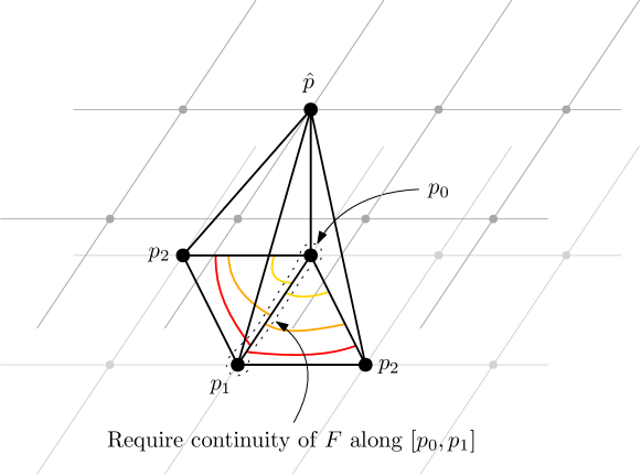
Figure 5: A problem with mp0 for which we provide a simple solution. The cost function $F$ must be continuous across the boundaries of adjacent update simplexes, otherwise an inconsistent solver can come about. Here, the colorered level sets depict the discontinuity of $F_{\operatorname{mp0}}$ across the bases of the update simplexes. In this case, two adjacent update simplexes share a common boundary on their base, shown here as the line segment $[p_{0},p_{1}]$. Two layers of surrounding grid points from $\mathcal{G}$ are shown. The point $\hat{p}$ is in the top layer and the points $p_{0}$, $p_{1}$, and $p_{2}$ are in the bottom layer.

If we use $F_{\operatorname{mp0}}$ directly, then we run into a situation where the cost function $F_{\operatorname{mp0}}$ is not continuous between the bases of adjacent update simplices (see fig. 5). We require $F$ to be continuous across simplex boundaries to avoid an inconsistent or divergent solver. Now, if we first use $F_{\operatorname{mp0}}$ to compute the minimizer $\lambda_{0}^{*}$ of eq. 14 with $F=F_{\operatorname{mp0}}$, and then set $\hat{U}=F_{\operatorname{mp1}}(\lambda_{0}^{*})$, we will recover continuity, and indeed, as we will show, the scheme is convergent. The motivation this is that eq. 14 can be solved exactly for the $\theta$-rule $F_{0}$ using a QR decomposition instead of an iterative solver, making it very cheap. In the next section, we will show how this can be done.

Let $\lambda_{0}^{*}$ and $\lambda_{1}^{*}$, denote the optima of eq. 14, where $F=F_{0}$ and $F=F_{1}$ (the general $\theta$-rules), respectively. We could imagine using Newton’s method to minimize $F_{1}$, starting from $\lambda_{0}^{*}$ (to be clear, this is not the approach we will ultimately take numerically). This would allow us to use the convergence theory of Newton’s method to bound the distance between $\lambda_{0}^{*}$ and $\lambda_{1}^{*}$, thereby bounding the error incurred by using mp0 instead of mp1 to find the minimizing argument of eq. 14. We follow this idea now.

Theorem 3.1

Using lemma 2, let $h$ be sufficiently small so that $F_{1}$ is strictly convex. Then, the error ${\delta\lambda}^{*}=\lambda_{1}^{*}-\lambda_{0}^{*}$ satisfies $\left\|{\delta\lambda}^{*}\right\|=O(h)$. Further, if we let $\lambda_{0}=\lambda_{0}^{*}$ in the following Newton iteration:

$$\lambda_{k+1}\leftarrow\lambda_{k}-\nabla^{2}F_{1}(\lambda_{k})^{-1}\nabla F_{1}(\lambda_{k}),\qquad k=0,1,\ldots,$$ (20)

then this iteration is well-defined, and converges quadratically to $\lambda_{1}^{*}$. This immediately implies that the error incurred by mp0 is $O(h^{3})$ per update compared to mp1; i.e.:

$$\left|F_{1}(\lambda_{1}^{*})-F_{1}(\lambda_{0}^{*})\right|=O(h^{3}).$$ (21)

Proof

The proof of theorem 3.1 is detailed in appendix D.

We will show in the next section how $\lambda_{0}^{*}$ can be computed directly using a QR decomposition and without using an iterative solver.

We can provide some intuition for why this bound is satisfactory. If we assume that our domain is spanned along a diameter by $O(N)$ nodes, and that $h\sim N^{-1}$, then we can anticipate $O(N)$ downwind updates, starting from bd and extending to the boundary of $\mathcal{G}$ in any direction. Accumulating the error over these nodes, we can expect the maximum pointwise error between a solution to eq. 1 computed by using mp0 and mp1 to be $O(h^{2})$, which is dominated by the $O(h)$ discretization error coming from the linear convergence of the method itself. Hence, using mp0 instead of mp1 only to find the parameter $\lambda$, and then evaluate $\hat{U}$ using $F_{1}$, should introduce no significant extra error.

3.4 Exact solution for rhr and mp0 using a QR decomposition

Since $F_{0}$ is strictly convex, $\nabla F_{0}(\lambda)=0$ is sufficient for the optimality of $\lambda$, ignoring the constraint $\lambda\in\Delta^{d}$. The unconstrained system of nonlinear equations defined by $\nabla F_{0}(\lambda)=0$ can be solved exactly without an iterative solver. We can compute the solution using the reduced QR decomposition of ${\delta P}$ and by considering the problem’s geometry (see also figure 21, in the appendix). This is captured in the following theorem. We will discuss how to use this theorem efficiently in a solver in section 4.4.

Theorem 3.2

Let ${\delta P}=QR$ be the reduced QR decomposition of ${\delta P}$; i.e., where $Q\in\mathbb{R}^{n\times d},R\in\mathbb{R}^{d\times d},Q^{\top}Q=I_{d}$, and with $R$ upper triangular. For $s^{\theta},h$, and $U$ fixed, if $\lambda^{*}=\operatorname{argmin}_{\lambda\in\mathbb{R}^{n}}F_{0}(\lambda)$, then:

$$\|p_{\lambda^{*}}\| =\sqrt{\frac{p_{0}^{\top}{(I-QQ^{\top})}p_{0}}{1-\left\|R^{-\top}\frac{{\delta U}}{s^{\theta}h}\right\|^{2}}},$$ (22)

$$\lambda^{*} =-R^{-1}\left(Q^{\top}p_{0}+\|p_{\lambda^{*}}\|R^{-\top}\frac{{\delta U}}{s^{\theta}h}\right),$$ (23)

$$\hat{U} =U_{0}+\frac{s^{\theta}h}{\|p_{\lambda^{*}}\|}p_{0}^{\top}p_{\lambda^{*}}.$$ (24)

Proof

See section E.

3.5 Equivalence of the upwind finite difference scheme and $F_{0}$

If we linearly approximate $U$ near $\hat{p}$, then for $i=0,\ldots,n-1$, we find that $\hat{U}$ satisfies:

$$U_{i}-\hat{U}=\nabla\hat{U}^{\top}p_{i}.$$ (25)

This finite difference approximation to eq. 1 can be solved exactly and is a known generalization of the upwind finite difference scheme used in the fast marching method on an unstructured mesh kimmel1998computing ; sethian2000fast . Computing $\hat{U}$ using this approximation is equivalent to solving:

$$\hat{U}=\min_{\lambda\in\Delta^{n}}F_{0}(\lambda)$$ (26)

in a sense made precise by the following theorem. As we have pointed out, this theorem is not new, but we present it here for the sake of continuity and because it dovetails with our other theorems, providing context.

Theorem 3.3 (Equivalence of upwind finite difference scheme and $F_{0}$)

Let $\hat{U}$ by the solution of eq. 25 and let $\hat{U}^{\prime}=\min_{\lambda\in\mathbb{R}^{n}}F_{0}(\lambda)$. Then, $\hat{U}$ exists if and only if $\|R^{-\top}{\delta U}\|\leq s^{\theta}h$, and can be computed from:

$$\hat{U}=U_{i}-p_{i}^{\top}QR^{-\top}{\delta U}+\left\|p_{\operatorname{min}}\right\|\sqrt{{(s^{\theta}h)}^{2}-\left\|R^{-\top}{\delta U}\right\|^{2}},$$ (27)

where $p_{\operatorname{min}}=(I-QQ^{\top})p_{i}$ (for all $i=0,\ldots,n-1$—see figure 21 in section E). Additionally, the following hold:

1. The finite difference solution and line integral solution coincide: i.e., $\hat{U}=\hat{U}^{\prime}$ can be computed from:

   $$\hat{U}=U_{i}+s^{\theta}hp_{i}^{\top}\nu_{\lambda^{*}},$$ (28)

   where $\lambda^{*}=\operatorname{argmin}_{\lambda\in\mathbb{R}^{n}}F_{0}(\lambda)$ and $\nu_{\lambda^{*}}=p_{\lambda^{*}}/\|p_{\lambda^{*}}\|$.

2. The characteristics found by solving the finite difference problem and minimizing $F_{0}$ coincide and are given by $[p_{\lambda^{*}},\hat{p}]=[p_{\lambda^{*}},0]$.

3. The approximated characteristic passes through $\operatorname{conv}(\left\{p_{0},\ldots,p_{n-1}\right\})$ if and only if $\lambda^{*}\in\Delta^{n}$.

Proof

See section F.

3.6 Causality

Dijkstra-like methods are based on the idea of monotone causality, similar to Dijkstra’s method itself. To compute shortest paths in a network, Dijkstra’s method uses dynamic programming to compute globally optimal shortest paths using local information dijkstra1959note . In this way, the distance to each downwind vertex must be greater than its upwind neighboring vertices. To ensure convergence to the correct viscosity solution, our scheme must be consistent and monotone crandall1983viscosity . Our OLIMs using the rhr quadrature rule inherit the consistency and causality of the finite difference methods which they are equivalent to if they use the same 4 (in 2D) or 6 (in 3D) point neighborhoods. Since we consider many different update neighborhoods involving distinct simplexes, we provide a simple way of checking whether each simplex is causal.

The causality of an update depends on the underlying simplex and the problem data. In particular, an update is causal for $F_{i}$ if:

$$\hat{U}=F_{i}(\lambda_{i}^{*})\geq\max_{i}U_{i}.$$ (29)

It is enough to determine whether or not each type of update simplex admits only causal updates, which relates to whether the simplex is acute.

We also consider something we refer to here as the “update gap”: the difference $\hat{U}-\max_{i}U_{i}$. As discussed in Tsitsiklis’s original paper tsitsiklis1995efficient , an alternative to Dijkstra’s algorithm is Dial’s algorithm—a bucketed version of Dijkstra’s algorithm which runs in $O(N^{n})$ time, where the constant depends on the bucket size dial1969algorithm ; kim2001calo . In this case, the size of the buckets is determined by the update gap. It is unclear whether there is any real advantage of a Dial-like solver (see jeong2008fast for a discussion), although a new numerical study suggests that there may indeed be some advantage in using a Dial-like solver kim2001calo ; gomez2019fast . Despite this, the update gap is of fundamental importance and limits the number of nodes that can be processed in parallel without violating causality.

Theorem 3.4

For $\nu_{i}=p_{i}/\|p_{i}\|$, an update simplex is causal for $F_{0}$ if and only if $\nu_{i}^{\top}\nu_{j}\geq 0$ for all $i$ and $j$ such that $0\leq i<n$ and $0\leq j<n$. The update gap is given explicitly by:

$$\hat{U}-\max_{i}U_{i}=s^{\theta}h\min_{i,j}\frac{\nu_{i}^{\top}\nu_{j}}{\left\|p_{i}\right\|}.$$ (30)

If we assume that $s$ is Lipschitz continuous, then for $h$ small enough, the simplex is also causal for $F_{1}$, and the term in $F_{1}$ which prevents an update from being causal decays with order $O(h^{2})$.

Proof

See section G.

In section 4.2 we present a table of update gaps for all update simplices considered in this paper.

The fact that our methods are causal for all practical problem sizes follows from the fact that the term preventing causality decays rapidly—see eq. 99. This can be seen easily by rewriting $F_{1}(\lambda)$ as $F_{0}(\lambda)$ plus a small perturbation (which is $O(h^{2})$) and using the Lipschitz continuity of $s$.

3.7 Local factoring

Near rarefaction fans, for example if $D$ is a point source or the domain contains obstacles with corners, the rate of convergence of the eikonal equation is diminished. For the eikonal equation with point source data and constant slowness, this degrades the rate of convergence to $O(h\log h^{-1})$ qi2018corner ; zhao2005fast . Fast sweeping methods for the factored eikonal equations have been developed fomel2009fast ; luo2012fast ; likewise, fast marching methods have been developed, and have also been used in the context of travel time tomography qi2018corner ; treister2016fast .

In this section, we show how the ordered line integral method can be easily adapted to additive factoring, and provide numerical tests that show that it recovers the expected linear rate of convergence for factored point source problems. Our focus is locally factored point sources, but this approach can be applied to the globally factored equation and other types of rarefaction fans occuring at corners or discontinuities qi2018corner .

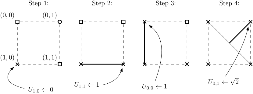
Figure 6: An example of running olim4_rhr with local factoring for three steps. Note that olim4_rhr is equivalent to the standard 2D fast marching method. We assume $s\equiv 1$. Initially, $p^{\circ}=p_{1,0}$ is the only node in bd and is factored. The first two steps proceed exactly the same as for the unfactored method, since the steps between the source nodes and the updated nodes lie along characteristics. In the third step, the unfactored method would set $U_{0,1}\leftarrow 1+\nicefrac{{\sqrt{2}}}{{2}}$. However, for the factored solver, we find that $U_{0,1}\leftarrow\nicefrac{{\sqrt{2}}}{{2}}+\nicefrac{{\sqrt{2}}}{{2}}=\sqrt{2}$.

Let $x^{\circ}\in\Omega$ be the location of a point source so that $\texttt{bd}=\left\{x^{\circ}\right\}$, define $p^{\circ}$ to be the image of $x^{\circ}$ under the same transformation that takes $\hat{x}$ to $\hat{p}$, and let $s^{\circ}=s(x^{\circ})$. The additive factorization of $U$ around $x^{\circ}$ is luo2012fast ; qi2018corner :

$$U(x)=T(x)+\tau(x),\qquad\text{where}\qquad T(x)=s^{\circ}\left\|x-x^{\circ}\right\|,$$ (31)

i.e. $u_{\lambda}=T_{\lambda}+\tau_{\lambda}$ where $T_{\lambda}=s^{\circ}h\|p_{\lambda}-p^{\circ}\|$. Our original definition of $F_{i}$ was such that $\hat{U}=F_{i}(\lambda^{*})$. We will define $G_{i}$ analogously. Letting $\tau_{\lambda}=\tau_{0}+{\delta\tau}^{\top}\lambda$, where $\tau_{i}$ and $T_{i}$ are the values of $\tau$ and $T$ at $p_{i}$ for each $i$, we define:

$$G_{0}(\lambda) =\tau_{\lambda}+T_{\lambda}+s^{\theta}h\|p_{\lambda}\|,$$ (32)

$$G_{1}(\lambda) =\tau_{\lambda}+T_{\lambda}+s^{\theta}_{\lambda}h\|p_{\lambda}\|.$$ (33)

Like with $F_{0}$ and $F_{1}$, the only difference between $G_{0}$ and $G_{1}$ is between the terms containing $s^{\theta}$ and $s^{\theta}_{\lambda}$. We do not explicitly refer to them in the rest of this paper, but the cost functions $G_{\texttt{rhr}}$, $G_{\texttt{mp0}}$, and $G_{\texttt{mp1}}$ are defined analogously to $F_{\operatorname{rhr}}$, $F_{\operatorname{mp0}}$, and $F_{\operatorname{mp1}}$ from the $\theta$-rules $G_{0}$ and $G_{1}$.

To solve the factored eikonal equation, we choose a factoring radius $r^{\circ}$, replacing $F_{i}$ with $G_{i}$ in eq. 14 for nodes which lie within a distance $r^{\circ}$ of $x^{\circ}$. For constant slowness, the effect of this is to solve eq. 1 exactly inside of the locally factored region. For clarity, this is depicted in figure 6. Algorithm 2 can be applied to solve eq. 14 for factored nodes. The gradient and Hessian of $G_{i}$ are simple modifications of the gradient and Hessian for $F_{i}$.

Lemma 3

The gradient and Hessian of $G_{i}$ for $i=0,1$ are given by:

$$\nabla G_{i}(\lambda) =\nabla F_{i}(\lambda)-{\delta\tau}+\frac{s^{\circ}h}{\|p_{\lambda}-p^{\circ}\|}{\delta P}^{\top}{(p_{\lambda}-p^{\circ})},$$ (34)

$$\nabla^{2}G_{i}(\lambda) =\nabla^{2}F_{i}(\lambda)+\frac{s^{\circ}h}{\|p_{\lambda}-p^{\circ}\|}{\delta P}^{\top}\mathtt{Proj}^{\perp}_{p_{\lambda}-p^{\circ}}{\delta P}.$$ (35)

4 Implementation of the ordered line integral method

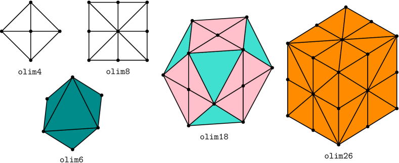
Figure 7: Neighborhoods for the top-down family of algorithms. Algorithms olim4 and olim8 are 2D solvers and the rest are 3D solvers. The color coding of tetrahedron updates is the same for this figure and figure 9 below.

Figure 8: Numbering scheme for update groups for the top-down solvers. In this diagram, $\hat{p}$ is being updated. The diagonally opposite node is the sixth (last) node, with the other six nodes numbered 0–5 cyclically.

0

$\bullet$

$\bullet$

$\bullet$

$\bullet$

$\bullet$

$\bullet$

$\bullet$

$\bullet$

$\bullet$

$\bullet$

1

$\bullet$

$\bullet$

$\bullet$

$\bullet$

$\bullet$

$\bullet$

$\bullet$

$\bullet$

$\bullet$

$\bullet$

2

$\bullet$

$\bullet$

$\bullet$

$\bullet$

$\bullet$

$\bullet$

$\bullet$

$\bullet$

$\bullet$

$\bullet$

3

$\bullet$

$\bullet$

$\bullet$

$\bullet$

$\bullet$

$\bullet$

$\bullet$

$\bullet$

$\bullet$

$\bullet$

4

$\bullet$

$\bullet$

$\bullet$

$\bullet$

$\bullet$

$\bullet$

$\bullet$

$\bullet$

$\bullet$

$\bullet$

5

$\bullet$

$\bullet$

$\bullet$

$\bullet$

$\bullet$

$\bullet$

$\bullet$

$\bullet$

$\bullet$

$\bullet$

I

II

III

IV

0

$\bullet$

$\bullet$

$\bullet$

$\bullet$

$\bullet$

1

$\bullet$

$\bullet$

$\bullet$

$\bullet$

$\bullet$

2

$\bullet$

$\bullet$

$\bullet$

$\bullet$

$\bullet$

3

$\bullet$

$\bullet$

$\bullet$

$\bullet$

$\bullet$

4

$\bullet$

$\bullet$

$\bullet$

$\bullet$

$\bullet$

5

$\bullet$

$\bullet$

$\bullet$

$\bullet$

$\bullet$

6

$\bullet$

$\bullet$

$\bullet$

$\bullet$

$\bullet$

$\bullet$

$\bullet$

$\bullet$

$\bullet$

$\bullet$

$\bullet$

$\bullet$

$\bullet$

$\bullet$

$\bullet$

V

VI

VII

Figure 9: Tables of update groups. These tables should be scanned columnwise: each column of dots selects a different tetrahedron. Tetrahedra (0, 1, 2), (2, 3, 4), and (4, 5, 0) in group I and all tetrahedra in group VII are degenerate and can be omitted.

In this section, we describe our bottom-up and top-down algorithms (see fig. 1). We focus on 3D solvers, since in 2D the distinction between the two is less important. Each algorithm reduces the number of updates that are done without degrading solution accuracy by using an efficient enumeration or search for update simplexes. The primary difference between the two algorithms is the ordering of the updates’ dimensions: top-down proceeds from $d=n-1$ down to $d=0$, skipping lower-dimensional updates when possible, and bottom-up proceeds from $d=0$ up to $d=n-1$, skipping higher-dimensional updates when it can.

4.1 Simplex enumeration for the top-down algorithm

When a node is first removed from front and has just become valid (item 3a in algorithm 1), an isotropic solver must do updates involving, at the very least, the node’s $2n$ nearest neighbors. We can use larger neighborhoods to improve the accuracy of the result. Doing so does not necessarily improve the order of convergence of the solver, but can significantly improve the error constant of the solution. For all of the solvers considered in this paper, in 3D, we only consider neighborhoods with at most 26 neighbors. See fig. 9 for neighborhoods for the top-down solver.

For the top-down solver, we simplify things by only doing updates which have $p_{i}=p_{\operatorname{new}}$ for some $i$. To iterate over all update simplexes, by symmetry, we enumerate all simplexes in a single octant. This means enumerating, e.g., ${7\choose 3}=35$ tetrahedra. Some choices lead to degenerate tetrahedra, so the number of nondegenerate update tetrahedra is fewer than 35 per octant. This makes it reasonable to write out the update procedure as straight-line code.

We enumerate the tetrahedra in a type of “shift-order” (see, e.g., arndt2010matters )—that is, we start with an unseen bit pattern, and group this pattern together with all of its shifts (with rotation). This groups the tetrahedra into sets that are rotationally symmetric about the diagonal of the octant. In our implementation, we conditionally compile different groups so that no unnecessary branching is done. This is done using C++ templates stroustrup2013c++ . Example stencils for the versions of olim6, olim18, and olim26 that are used for our numerical test are shown in figure 9. The tetrahedron groups are shown in figures 9 and 9.

4.2 Update gaps for tetrahedron groups

If we apply theorem 3.4 to the tetrahedron groups enumerated in figures 9 and 9, we get the following update gaps, enumerated in the same order as fig. 9 (ignoring the $s^{\theta}h$ factor):

Group I	$\nicefrac{{1}}{{\sqrt{2}}}$	Group II	$\nicefrac{{1}}{{\sqrt{2}}}$	Group III	$\nicefrac{{1}}{{\sqrt{2}}}$	Group IVa	0
Group V	$\nicefrac{{1}}{{\sqrt{3}}}$	Group VIa	0	Group VIb	$\boldsymbol{\nicefrac{{2}}{{\sqrt{3}}}}$	Group IVb	$\nicefrac{{1}}{{\sqrt{2}}}$

The update gap is first explored in Tsitsiklis’s original paper tsitsiklis1995efficient ; in this work, the fact that Group IVa has no update gap and that the update gap of Group V is $1/\sqrt{3}$ is noted and an $O(N^{n})$ algorithm based on Dial’s algorithm is presented using Group V for the update tetrahedra. This same observation is made in a more recent paper about a method based on Dial’s algorithm kim2001calo . A method based on a combination of tetrahedra groups will have an update gap that is the minimum of each of the individual groups’ gaps. We note here that a solver based on a combination of Groups I and VIb has a larger update gap than a solver based on Group V. This should have a positive impact on the performance of any parallel Dijkstra-like method.

4.3 The search procedure used by the bottom-up algorithm

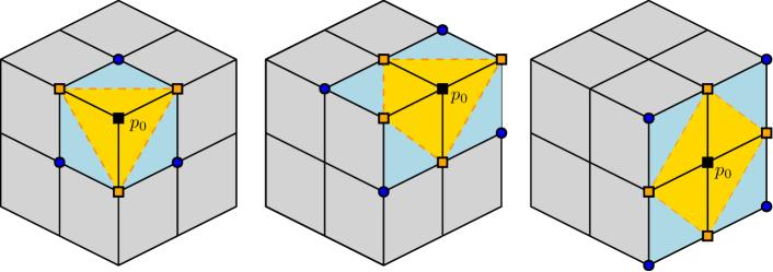
Figure 10: The three types of neighborhoods for the bottom-up algorithm. The yellow and blue regions indicate where triangle and tetrahedron updates may be performed, respectively. For instance, with $p_{0}$ the minimizing line update vertex, candiates for $p_{1}$ consist of the yellow nodes: triangle updates involving these candidates and $p_{0}$ will be performed. Once a yellow node ($p_{1}$) has been selected, tetrahedron updates involving the neighboring blue nodes (candidates for $p_{2}$) will be performed. Note that the updates performed correspond roughly to a combination of groups I, V, VIa, and VIb.

Figure 11: Skipping lower-dimensional updates when solving the unconstrained minimization problem. For $d=2$, if $\lambda_{0}^{*}\in\Delta^{2}$, all three triangle updates can be skipped. On the other hand, when minimizing $F_{0}$ using theorem 3.2, if $\lambda^{*}_{0}\notin\Delta^{2}$ and depending on where $\lambda_{0}^{*}$ lies, it is possible to skip one or two triangle updates. In this case, we label the different regions by the number of updates that it is possible to skip: $\lambda^{*}$ here lies in “zone 2”, since it is possible to skip the two triangle updates on the opposite side of $\Delta^{2}$. Along the same lines, if $\lambda^{*}$ were to lie in “zone 1”, two triangle updates would be “visible”, and it would only be possible to skip one update.

Another approach is to use local characteristic information obtained by performing lower-dimensional updates to help us avoid performing unnecessary higher-dimensional updates. Intuitively, if we find the minimum line update ($d=0$), then we can avoid triangle updates ($d=1$) that don’t include the minimizing line update. Since we only perform updates for $d>0$ that include the newly valid node $p_{\operatorname{new}}$, we can start our search with $d=1$.

After doing an update of dimension $d$, we find neighboring updates of dimension $d+1$. For $n=3$ and $d=1$, for each $p_{0}$, we find points $p_{1}$ that satisfy $\|p_{0}-p_{1}\|_{1}\leq 1$. For $d=2$, for each pair $(p_{0},p_{1})$, we find points $p_{2}$ that satisfy $\|p_{0}-p_{2}\|_{1}\leq 2$ and $\|p_{1}-p_{2}\|_{1}\leq 2$ simultaneously. In practice, we only find these neighbors once and precompute an array of indices to be used later. The neighborhoods computed in this way are shown in fig. 10.

4.4 Minimization algorithms and skipping updates

When $F_{i}=F_{0}$, we can use theorem 3.2 or 3.3 to compute $\lambda_{0}^{*}$. If $F_{i}=F_{1}$, we need to use an algorithm that can solve the constrained optimization problem defined by eq. 14. Our approach has been to use sequential quadratic programming (SQP), although there are many other options bertsekas1999nonlinear ; nocedal2006numerical . It is possible to skip some updates; and, indeed, the performance of our algorithms comes about largely because of this happening.

We skip updates in three different ways. The first two approaches are used by the top-down algorithms, and the third by the bottom-up algorithms.

Top-down constrained skipping.

When computing an update using a constrained solver, we can rule out all incident lower-dimensional updates, since we have computed the global constrained optimum on $\Delta^{d}$.

Top-down unconstrained skipping.

If we do an update using an unconstrained solver, then depending on where the optimum $\lambda_{0}^{*}$ lies, we can skip some or all lower-dimensional updates. The idea is simple and is best depicted visually, see fig. 11.

Bottom-up KKT skipping.

We can also skip higher-dimensional updates. For example, if we do the three triangle updates on the boundary of a tetrahedron update, we can use the Karush-Kuhn-Tucker necessary conditions for optimality of a constrained optimization problem nocedal2006numerical to determine if the minimizer on the boundary is also a global minimizer for the constrained minimization problem given by eq. 14. See appendix B. We note that a modified version of this strategy for skipping updates was used in the work on computing the quasipotential for nongradient SDEs in 3D yang2019computing .

4.5 The bottom-up and top-down algorithms

Algorithm 2 The top-down algorithm.

1. Set $\hat{U}\leftarrow\infty$.

2. Initialize $\mathcal{V}_{d}$ according to eq. 36 for each $d=0,\ldots,n-1$.

3. For $d=n-1$ down to $0$:

   1. For each $(p_{0},\ldots,p_{d})\in\mathcal{V}_{d}$:

      1. If $F_{i}=F_{0}$ (mp0 or rhr):

         1. Compute $U$ for $(p_{0},\ldots,p_{d})$ using theorem 3.2 or 3.3.

         2. Remove updates from $\mathcal{V}_{0},\ldots,\mathcal{V}_{d-1}$ by visibility (see figure 11).

      2. Otherwise, if $F_{i}=F_{1}$ (mp1):

         1. Compute $U$ by solving eq. 14 numerically (we use SQP).

         2. Remove all lower-dimensional updates from $\mathcal{V}_{0},\ldots,\mathcal{V}_{d-1}$.

      3. Set $\hat{U}\leftarrow\min(\hat{U},U)$.

Algorithm 3 The bottom-up algorithm.

1. Set $\hat{U}\leftarrow\infty$ and $p_{0}\leftarrow p_{\operatorname{new}}$.

2. For $i=1,\ldots,n-1$:

   1. For each valid $p_{i}$ close enough to $p_{0},\ldots,p_{i-1}$ (see section 4.3), do the update corresponding to $(p_{0},\ldots,p_{i})$ and keep track of the minimizing $\lambda^{*}\in\Delta^{i}$. This update can optionally be skipped by first computing $\mu^{*}$ corresponding to the optimum of the incident lower-dimensional update $(p_{0},\ldots,p_{i-1})$ and checking if $\mu^{*}\geq 0$.

   2. Let $p_{i}$ be the node which forms the update with the minimum value.

   3. If $F_{i}=F_{0}$ (mp0 or rhr), compute $U$ for $(p_{0},\ldots,p_{i})$ using theorem 3.2 or 3.3.

   4. Otherwise, if $F_{i}=F_{1}$ (mp1), compute $U$ for $(p_{0},\ldots,p_{i})$ by solving eq. 14.

   5. Set $\hat{U}\leftarrow\min(\hat{U},U)$.

In this section, we describe our bottom-up and top-down algorithms. We note for clarity that these algorithms correspond to the “compute $\hat{U}$” part of item 3d of alg. 1.

To describe our top-down algorithm (see algorithm 2), we define the set of admissible $d$-dimensional updates neighboring the point $\hat{p}$ by:

$$\mathcal{V}_{d}=\big{\{}\left\{p_{0},\ldots,p_{d}\right\}: p_{i}\texttt{.state}=\texttt{valid}\mbox{ for }i=0,\ldots,d,$$ (36)

$$\mbox{and}\left\{p_{0},\ldots,p_{d}\right\}\mbox{are in a selected update group},$$

$$\mbox{and }p_{\operatorname{new}}\in\left\{p_{0},\ldots,p_{d}\right\}\big{\}}$$

for $d=0,\ldots,n-1$. The update set $\mathcal{V}_{d}$ collects all admissible simplex updates of a given dimension: i.e., updates which both belong to a group as defined in section 4.1 and are valid. The third condition is an important optimization. To see why it is correct, fix an update set $\mathcal{V}_{d}$. If $\left\{p_{0},\ldots,p_{d}\right\}$ satisfies the first two conditions but not the third, we can see that $\hat{p}$ would have already been updated from it in a previous iteration. All new information affecting $\hat{U}$ during this iteration must be computed from an update involving $p_{\operatorname{new}}$.

The bottom-up algorithm (algorithm 3) builds up each update $(p_{0},\ldots,p_{d})$ one vector at a time by searching for adjacent minimizing updates of higher dimension. The optimization involving $p_{\operatorname{new}}$ described above can be incorporated by initially setting $p_{0}\leftarrow p_{\operatorname{new}}$.

5 Numerical Results

We do tests involving several different slowness functions with analytic solutions for point source data, and a linear speed function (i.e., $1/s$) which has been shown to be amenable to local factoring. For each quadrature rule described in section 3.1 (mp0, mp1, or rhr), we have two 2D algorithms, olim4 and olim8, corresponding to 4- and 8-point stencils, respectively. Since there is no advantage in 2D, we don’t apply the top-down or bottom-up approaches. In 3D, we have three top-down algorithms: olim6 (group IVa), olim18 (groups I, IVa, and IVb), and olim26 (group V). We also test the bottom-up algorithm olim3d (see figure 10).

5.1 Implementation Notes

Figure 12: Slowdown incurred by using olim6_rhr instead of the FMM. From left to right: 1) the ratio of runtimes versus $N$, 2) the total CPU runtime of each solver. We compare results on two different computers: “2.2 GHz” is a 2015 MacBook Air with a 2.2 GHz Intel Core i7 CPU, 8 GB of 1600 MHz DDR3 RAM, a 256 KiB L2 cache, and a 4 MiB L3 cache; “4.6 GHz” is a custom built workstation running Linux with a 4.6 GHz Intel Core i7 CPU, 64 GB of 2133 MHz DDR4 RAM, a 1536 KiB L2 cache, and 12 MiB L3 cache. Both computers have 32 KiB L1 instruction caches and data caches. The plots here use our standard $\Omega=[-1,1]^{3}$ domain discretized into $N=2^{p}+1$ nodes in each direction, with $s\equiv 1$ and a point source at the origin.

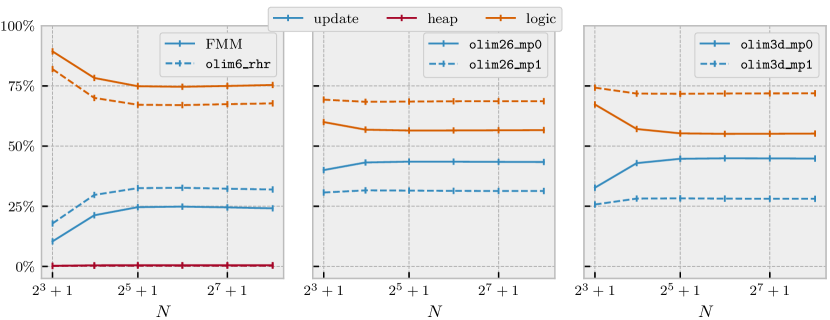
Figure 13: Percentage of time spent on different tasks as determined by profiling. The “update” tasks and “heap” tasks are clearly defined, while the “logic” task contains a variety of things related to control-flow, finding neighbors, and memory movement—basically, the parts of algorithm 1 that don’t clearly pertain to computing new $\hat{U}$ values or keeping front updated. From these plots, it is clear that memory speed plays a large role in determining efficiency. To some extent, even though the more complicated update procedures are slower, their slowness is hidden somewhat by memory latency as problem sizes grow. For large $N$ and some solvers (the middle and right plots), “heap” takes too little time, and is not picked up by the profiler.

Before describing our numerical tests, we briefly comment on our implementation and make some observations about its performance. A discussion of some of the choices that we made in our implementation follows:

• We precompute and cache all values of $s$ on the grid $\mathcal{G}$, as opposed to reevaluating $s$, because we assume that $s$ will be provided as gridded data (consider, e.g., the shape from shading problem kimmel2001optimal , where the input data is an image).

• We maintain front using a priority queue implemented using an array-based binary heap, which is updated using the sink and swim functions described in Sedgewick and Wayne sedgewick2011algorithms .

• We store front as a dense grid of states: for each node in $p\in\mathcal{G}$, we track $p$.state for all time for every node. We could implement a sparse front using a hash map or a quadtree or octree, which would save space, but would also be much slower to update.

We use a policy-based design alexandrescu2001modern written in C++. This allows us to conditionally compile different features and reuse logic to implement different Dijkstra-like algorithms. In particular, we implement the standard FMM sethian1996fast and make a direct comparison between it and the ordered line integral method which it is equivalent to, olim6_rhr (see figure 12). We have found that only a modest slowdown is incurred by using olim6_rhr for problems of moderate size. The disparity between the two is greater for smaller problem sizes, which is due to cache effects. In general, the difference in speed is due to the fact that the FMM’s update is extremely simple since it requires only the solution of quadratic equations.

Using Valgrind nethercote2007valgrind , we profiled running our solver on the numerical tests below for different problem sizes and categorized the resulting profile data. See figure 13. The “update” task corresponds to time spent actually computing updates, the “logic” task is a grab bag category for time spent on program logic, and “heap” corresponds to updating the array-based heap which implements front. Since the asymptotic complexity of the “update” and “logic” sections is $O(N^{n})$, and since “heap” is $O(N^{n}\log N)$, we can see from figure 13 that since so little time is spent updating the heap, the algorithm’s runtime is better thought of as $O(N^{n})$ for practical problem sizes (although this obviously not technically correct!). This is a consequence of using an array-based heap whose updates are cheap and cache friendly, and a dense grid of states, which can be read from and written to in $O(1)$ time.

As an aside, we mention that thorough numerical studies of eikonal solvers in the literature have been scarce, but we can point out a recent study which seeks to close this gap gomez2019fast . Our studies profiling our implementation using Valgrind are carried out in the same spirit as this work.

5.2 Slowness functions with an analytic solution for a point source

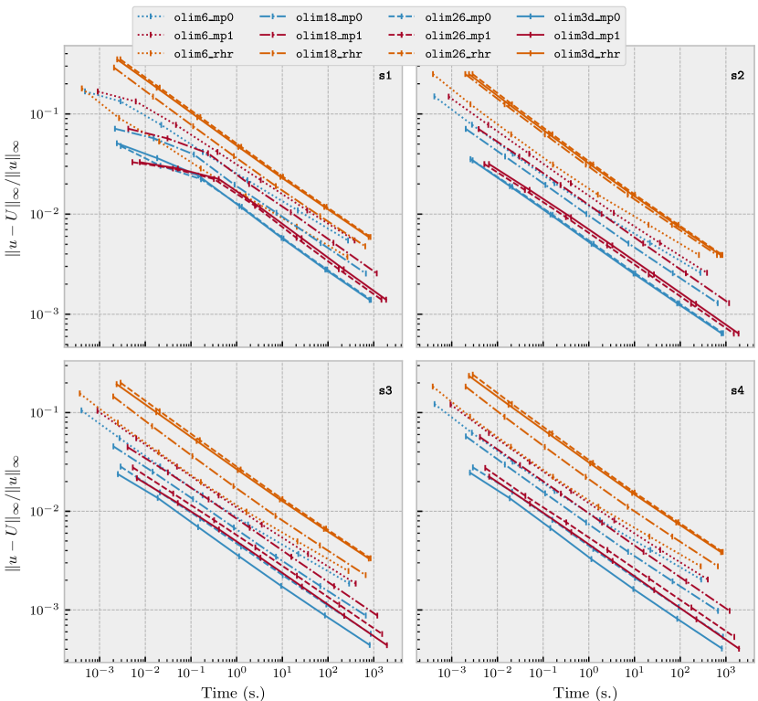
Figure 14: Relative $\ell_{\infty}$ error plotted against CPU runtime in seconds. The domain is $\Omega=[-1,1]^{3}$ discretized uniformly in each direction into $N=2^{p}+1$ points, where $p=3,\ldots,9$, so that there are $N^{3}$ points overall. The slowness functions used are listed in section 5.2. We note that the horizontal and vertical axes of each subplot are the same.

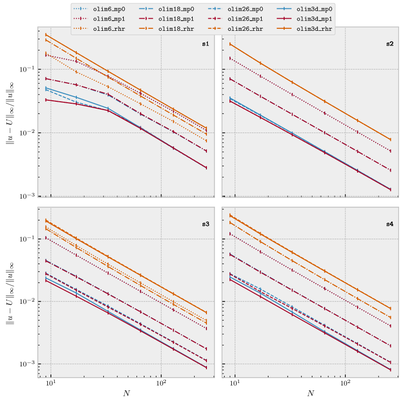
Figure 15: Relative $\ell_{\infty}$ error plotted versus $N$. The setup is the same as in figure 14, except that $p=3,\ldots,8$, so that the largest $N$ is $257$ instead of $513$. For olim26 and olim3d, we can see that mp0 is initially less accurate than mp1 but quickly attains parity, in accordance with theorem 3.1. For olim6 and olim18, the error is the same between mp0 and mp1 for all slowness functions, so these plots overlap.

Using eq. 1 directly, a simple recipe to create pairs of slowness functions and solutions is to prescribe a continuous function $u$ whose level sets are each homeomorphic to a ball and compute $s(x)=\left\|\nabla u(x)\right\|_{2}$ analytically, which is valid for a single point source at the origin. Such tests allow us to observe the effect of local factoring, and to see how mp0, mp1, and rhr compare. The following table lists our test functions:

Name	$u(x)$	$s(x)$
s1	$\cos(r)+r-1$	$1-\sin(r)$
s2	$r^{2}/2$	$r$
s3	$S(x)^{\top}AS(x)$	$\alpha\left\|\operatorname{diag}(C(x)){(A+A^{\top})}S(x)\right\|$
s4	$\tfrac{1}{2}x^{\top}A^{1/2}x$	$\left\|x\right\|_{A}=\sqrt{x^{\top}Ax}$

We assume that $x\in\Omega=[-1,1]^{3}$. We also define $r=\left\|x\right\|$, and vector fields $S(x)=(\sin(\alpha x_{i}))_{i=1}^{3}$ and $C(x)=(\cos(\alpha x_{i}))_{i=1}^{3}$; we take $\alpha=\pi/5$. For s3 and s4, we assume that $A$ is symmetric positive definite. In 3D, the matrices we use for s3 and s4 are:

$$A_{\texttt{s3}}=\begin{bmatrix}1&\nicefrac{{1}}{{4}}&\nicefrac{{1}}{{8}}\\ \nicefrac{{1}}{{4}}&1&\nicefrac{{1}}{{4}}\\ \nicefrac{{1}}{{8}}&\nicefrac{{1}}{{4}}&1\end{bmatrix}=A_{\texttt{s4}}^{1/2}$$ (37)

Our results are displayed in figures 14 and 15. We include the relative $\ell_{\infty}$ error versus problem size and time, as well as the $\ell_{\infty}$ error versus $N$. We summarize our observations:

• Using either of the midpoint rules (mp0 or mp1) allows improved directional coverage to translate into an improved error constant. See figs. 15 and 14.

• For rhr, increased directional coverage (olim6_rhr $\to$ olim18_rhr $\to$ olim26_rhr) does not lead to an improved error. In fact, for s1, s3, and s4, increasing the directional coverages causes the accuracy to deteriorate (see figure 15). This may be due to the fact that quadrature error and linear interpolation error have different signs, and may partially compensate each other (e.g., in olim6). This effect may get worse with increased directional coverage.

• If we scan each graph horizontally, focusing on the plot markers, we can see that the difference in error between mp0 and mp1 is minimal. For each mp1 graph, the corresponding mp0 graph has the same error, but is shifted to the left, reflecting the fact that the mp0 OLIMs are substantially faster. This is consistent with theorem 3.1, which justifies the use of mp0. See fig. 14.

• With respect to the choice of neighborhood, olim6 is the fastest; and, for each choice of neighborhood, mp0 provides the best combination of speed and accuracy. See fig. 14. If we are willing to pay somewhat in speed, we can dramatically improve the error constant by improving the directional coverage and using a solver like olim3d_mp0. This tradeoff is more pronounced for smaller problem sizes. A theme running through this work is that, as the problem size increases, memory access patterns come to dominate the runtime, and the disparity in runtimes between the faster and slower neighborhoods becomes less pronounced. To see this, compare the start of each graph in the top-left of the plots, and their ends in the bottom-right (again, see fig. 14). We can observe, e.g., that the maximum horizontal distance between starting points and ending points has decreased significantly, which confirms this observation.

• Our high accuracy algorithms allow us to obtain a better solution on rough grids: this is helpful since opportunities to refine the mesh are limited in 3D. Discretizing $\Omega=[-1,1]^{2}$ in each direction into $N=2^{14}+1$ nodes requires about as much memory as discretizing $\Omega=[-1,1]^{3}$ with $N=2^{9}+1$, which leads to $h$ being 32 times smaller in 2D than in 3D.

• In general, olim26 and olim3d are significantly more accurate than olim6 and olim18.

5.3 A linear speed function

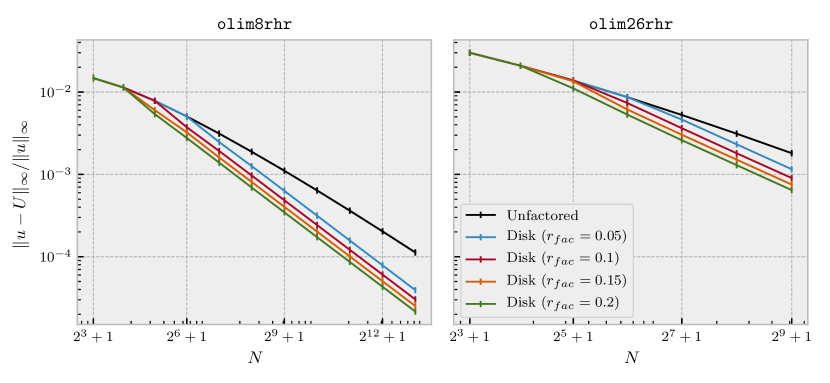
Figure 16: Comparing different ways of selecting factored nodes. For the test problem, $\Omega=[-1,1]^{n}$, with $n=2$ (left) and $n=3$ (right). The domain is descretized into $N^{3}$ nodes, where $N=2^{p}+1$, so that $h=2/(N-1)$. The slowness function is constant ($s\equiv 1$). For the 2D problem, olim8_rhr is used; olim26_rhr is used for the 3D problem. Solutions for the unfactored problem are plotted, along with solutions using a disk/sphere neighborhood with constant factoring radius given by $r^{\circ}=0.05,0.1,0.15,0.2$. We note that for this problem the choice $r^{\circ}=\sqrt{n}$ results in an exact solution. This only applies to the constant slowness function, $s\equiv 1$.

We consider a problem that has a known analytical solution and has been used as a test problem for other factored eikonal equation solvers before slotnick1959lessons ; fomel2009fast ; qi2018corner . For a single point source at $x_{i}$ and a vector $v$, we define:

$$\frac{1}{s(x)}=\frac{1}{s(x_{i})}+v^{\top}{(x-x_{i})},,$$ (38)

where $s_{i}=s(x_{i})$. The analytic solution to eq. 1 for a single source and slowness function given by eq. 38 is slotnick1959lessons :

$$u_{i}(x)=\frac{1}{\left\|v\right\|}\cosh^{-1}\left(1+\frac{s_{i}}{2}s(x)\left\|v\right\|^{2}\left\|x-x_{i}\right\|^{2}\right).$$ (39)

If we shift the point source from $x_{i}$ to another location $x_{j}$, we find:

$$\frac{1}{s_{i}}+v^{\top}{(x-x_{j}+x_{j}-x_{i})}=\frac{1}{s_{i}}+v^{\top}{(x_{j}-x_{i})}+v^{\top}{(x-x_{j})}=\frac{1}{s_{j}}+v^{\top}{(x-x_{j})}.$$ (40)

That is, the slowness function $s$ remains unchanged as it is rewritten with respect to a different source.

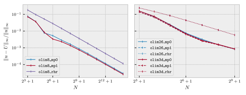
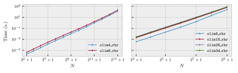
Figure 17: Numerical results for the linear speed function of section 5.3. Problem sizes are $N=2^{p}+1$, where $p=3,\ldots,14$ in 2D and $p=3,\ldots,9$ in 3D. The total number of nodes is $N^{n}$, where $n=2,3$. See section 5.3 for least squares fits. Top row: relative $\ell_{\infty}$ error plotted versus $N$ in 2D (left) and 3D (right). Bottom row: wall clock time plotted versus $N$ in 2D (left) and 3D (right).

If $\left\{x_{i}\right\}$ is a set of point sources and $u_{i}(x)$ is the solution of the eikonal equation for the single point source problem with point source given by $x_{i}$, then the solution for the multiple point source problem with sources $\left\{x_{i}\right\}$ is:

$$u(x)=\min_{i}u_{i}(x).$$ (41)

We use this formula to compare relative $\ell_{\infty}$ errors for each of our OLIMs in 2D and olim26 and olim3d in 3D for this slowness function with a pair of point sources, $x_{1}=(0,0)$ and $x_{2}=(0.8,0)$ in 2D, and $x_{1}=(0,0,0)$ and $x_{2}=(0.8,0,0)$ in 3D. We set the domain of the problem to be $\Omega=[0,1]^{n}$ and discretize it into $N=2^{p}+1$ points, so that $h=(N-1)^{-1}$.

For this choice of slowness function, we plot the CPU runtime versus $N$ (see figure 17), along with the relative $\ell_{\infty}$ error versus $N$ (see figure 17). We also do least squares fits for these plots to get an overall sense of the accuracy and speed (see 1).

We can see that our conclusions from section 5.2 also hold for the multiple point source problem. Additionally, our least-squares fits (table 1) indicate to us that our algorithms’ runtimes are accurately described by the fit $T_{N}\sim C_{T}N^{\alpha}$ with $\alpha\approx n$, and the error by $E_{N}\sim C_{E}h^{\beta}$, with $\beta\approx 1$ (here, $E_{N}$ is the relative $\ell_{\infty}$ error). In fact, for olim26 and olim3d with mp0 or mp1, the power $\beta$ is improved beyond $1$ to $\beta\approx 1.3$.

Neighborhood	$C_{T}$	$\alpha$
olim4	$7.779\times 10^{-8}$	1.0785
olim8	$1.971\times 10^{-7}$	1.0515
olim6	$2.968\times 10^{-7}$	1.085
olim18	$2.984\times 10^{-6}$	1.018
olim26	$4.649\times 10^{-6}$	1.0103
olim3d	$3.923\times 10^{-6}$	1.013

(a) $T_{N}\sim C_{T}N^{\alpha n}$

Neighborhood	$C_{E}$	$\beta$
olim8_mp0	0.4077	0.98744
olim8_mp1	0.3683	0.993
olim8_rhr	1.511	0.9728
olim26_mp0	2.328	1.3135
olim26_mp1	1.949	1.2888
olim26_rhr	1.772	0.90394
olim3d_mp0	2.268	1.3141
olim3d_mp1	1.865	1.2885
olim3d_rhr	1.77	0.90353

(b) $E_{N}\sim C_{E}h^{\beta}$

Table 1: Least-squares fits of the runtime and relative $\ell_{\infty}$ error for OLIMs in 2D and 3D. We denote the time for a given $N$ by $T_{N}$; likewise, $E_{N}$ denotes the relative $\ell_{\infty}$ error for a specific $N$. We fit $T_{N}$ to a power $C_{T}N^{\alpha}$. In 2D, we expect $\alpha\approx 2$; in 3D, $\alpha\approx 3$. In 3D, we fit $E_{N}$ to $C_{E}h^{\beta}$, and expect $\beta\approx-1$ in all cases, due to the use of local factoring. In fact, for olim26 and olim3d using either mp0 or mp1, we find that the situation is better than expected, with $\beta\approx-1.3$.

5.4 Marmousi velocity model tests

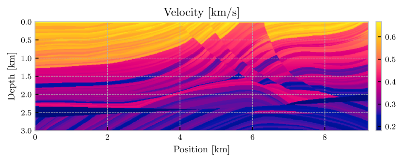
Figure 18: Marmousi slowness model. The original Marmousi model is given as a velocity model $c$. We work with $s=1/c$, so we plot this here. We also extrude this slowness model in the $y$ direction to create a 3D model.

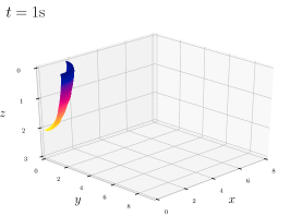
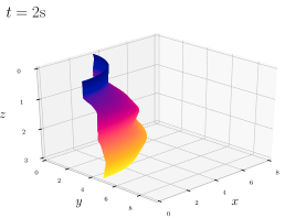
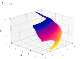
Figure 19: Level sets of $U$ (first arrival time) for $t=1$\mathrm{s}$,2$\mathrm{s}$,3$\mathrm{s}$$ for the extruded 3D Marmousi slowness model computed on a $94\times 288\times 288$ grid using olim3d_mp0. Distances are in $\mathrm{k}\mathrm{m}$. The level sets were computed using Lewiner’s version of the marching cubes algorithm lewiner2003efficient as implemented in scikit-image van2014scikit .

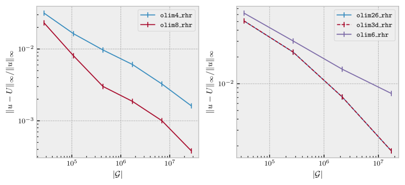
Figure 20: Relative $\ell_{\infty}$ errors for (unsmoothed) Marmousi point source problems in 2D and 3D using $F_{\operatorname{rhr}}$. The horizontal axis for each plot is the total number of grid nodes, $|\mathcal{G}|$. Left: 2D plots for olim4_rhr and olim8_rhr. Right: 3D plots for olim6_rhr, olim26_rhr, and olim3d_rhr. The 3D slowness model is obtained by extruding the original model in the $y$ direction. 2D Note that the plots for olim26_rhr and olim3d_rhr overlap.

A standard test problem in exploration geophysics is the Marmousi velocity model, which is a synthetic velocity model based on the North Quenguela Trough—see the following citation for more background information versteeg1994marmousi . The model consists of a number of stratified layers in the downward $z$ direction that are roughly piecewise constant. This model has been used frequently as a stress test for eikonal solvers, since the solution of the eikonal equation estimates the first arrival time of a seismic P-wave.

For 2D tests, if $c_{$\mathrm{m}$}(x,z)$ is the standard Marmousi velocity model in $\mathrm{m}\mathrm{/}\mathrm{s}$, we first convert to $\mathrm{k}\mathrm{m}\mathrm{/}\mathrm{s}$ and set $s(x,z)=1/c_{$\mathrm{k}\mathrm{m}$}(x,z)=1000/c_{$\mathrm{m}$}$. For the 3D tests, we just extrude the model in the $z$ direction, setting $s(x,y,z)\equiv s(x,z)$. We plot our slowness model in fig. 18. The domain used for 2D problems is $\Omega=[0,9.2]\times[0,3]$, and for 3D problems we set $\Omega=[0,9.2]\times[0,9.2]\times[0,3]$ (all distances in $\mathrm{k}\mathrm{m}$). For each test, we set $\texttt{bd}=\{0\}$. To get a sense of how a P-wave propagates in the extruded model, see fig. 19, where we plot several level sets at one second increments.

If we compare the quadrature rules defined in eq. 7, we can see that if:

$$\hat{s}=s_{0}=\cdots=s_{d}=\mbox{constant},$$ (42)

i.e., if an update is performed in a region that is locally constant, then $F_{\operatorname{rhr}}\equiv F_{\operatorname{mp0}}\equiv F_{\operatorname{mp1}}$. For the Marmousi model, we can expect this to occur in most regions, with the exception of updates that straddle two adjacent (approximately) piecewise constant regions. Naturally, our assumption that $s$ is Lipschitz breaks down for the Marmousi model.

In our numerical experiments, we have found $F_{\operatorname{rhr}}$ to handle this situation better than $F_{\operatorname{mp0}}$ or $F_{\operatorname{mp1}}$, although all of our solvers converge reasonably well for this model. We found that increased directional coverage does lead to signficantly improved accuracy. To demonstrate this phenomenon, we create a sequence of scaled Marmousi slowness models in 2D and 3D. In 2D, we used the sizes (288, 94), (575, 188), (1150, 376), (2301, 751), (4602, 1502), (9204, 3004), and (18408, 6008); in 3D, we used the sizes (144, 5, 47), (288, 10, 94), (575, 20, 188), (1150, 40, 376), (2301, 80, 751). In 2D, for our “ground truth” solution, we solve the problem at the finest resolution using olim8_rhr; for each of the smaller problem sizes, we downsample the groundtruth solution and compare with the solution computed using the smaller size to estimate the relative $\ell_{\infty}$ error. We do the same in 3D, but using olim3d_rhr. See fig. 20.

Additionally, we have included supplemental numerical experiments examining the behavior of different choices of quadrature rules on our solvers’ performance in 2D online marmousi-2d-online-supplement .

6 Conclusion

We have presented a family of fast and accurate direct solvers for the eikonal equation. The top-down algorithm relies on enumerating valid update simplexes, while the bottom-up algorithm employs a fast search for the first arrival characteristic. For each of these solvers, one can use different quadrature rules: a simplified midpoint rule (mp0), a midpoint rule (mp1), and a righthand rule (rhr).

We have analyzed the relationship between these quadrature rules, showing that the mp0 rule can be used to compute an approximate local characteristic direction, and $\hat{U}$ evaluated using this direction, while incurring only $O(h^{3})$ error per update, which justifies its use.

We have conducted extensive numerical experiments that show that olim3d_mp0 provides the best overall trade-off between runtime and error. We also compare the speed of the standard fast marching method in 3D with the equivalent olim6_rhr (equivalent in the sense that they compute the same solution to machine precision). We demonstrate that olim6_rhr incurs only a very modest overhead, suggesting that the top-down approach is an efficient way of generalizing the fast marching method; it also suggests that the bottom-up approach is a viable approach to speeding up Dijkstra-like algorithms in 3D, and should be viable for other types of algorithms that solve related equations (indeed, this has already been demonstrated for the quasipotential yang2019computing ).

To determine the relative time spent on different tasks, we have profiled our C++ implementation using Valgrind, separating time spent into several coarse-grained categories. From this, we show that for practical problem sizes, the runtime of Dijkstra-like algorithms behaves like $CN^{n}$, where $n=2,3$, and $N^{n}$ is the total number of gridpoints (even if this is not strictly true from a computational complexity viewpoint); we also emphasize that memory access patterns play a large role in algorithm runtime, especially for large $N$.

We conclude that ordered line integral methods are a powerful approach to obtaining a higher degree of accuracy when solving the eikonal equation in 3D. With an appropriate choice of quadrature rule, we are able to exploit improved directional coverage to drive down the error constant. The improved accuracy more than makes up for the modest price paid in speed, and we fully expect it to be possible to find ways to optimize this family of algorithms further. We have also attempted to demonstrate that memory access patterns dominate both update time and time spent maintaining the front data structure, from which we can conclude two things: 1) the exact time spent updating a node is important but not paramount (improving accuracy is more important than improving speed), 2) using memory optimally will lead to a substantial speed-up for large problems.

7 Acknowledgements

We thank Prof. A. Vladimirsky for valuable discussions during the course of this project.

Appendix A Minimum actional integral for the eikonal equation

The eikonal equation (eq. 1) is a Hamilton-Jacobi equation for $u$. If we let each fixed characteristic (ray) of the eikonal equation be parametrized by some parameter $\sigma$ and denote $p\equiv\nabla u$, the corresponding Hamiltonian is:

$$H{(p,x)}=\frac{\left\|p\right\|^{2}}{2}-\frac{s(x)^{2}}{2}=0.$$ (43)

Since $H=0$, eq. 43 implies $L=\sup_{p}(\langle p,x^{\prime}\rangle-H)=s(x)\left\|x^{\prime}\right\|$. Since $x^{\prime}=\partial_{p}H=p$ and $\left\|p\right\|=s(x)$ can be expressed as:

$$L(x,x^{\prime})=\langle p,x^{\prime}\rangle=\langle x^{\prime},x^{\prime}\rangle=\langle\nabla u,x^{\prime}\rangle=\frac{du}{d\sigma}.$$ (44)

Let $x(\sigma)$ be a characteristic arriving at $\hat{x}=x(\hat{\sigma})$ from $x_{0}=x(0)$, which lies on the expanding front. Integrating from $0$ to $\hat{\sigma}$ and letting $\hat{u}=u(\hat{x})$ and $u_{0}=u(x_{0})$:

$$\hat{u}-u_{0}=\int_{0}^{\hat{\sigma}}L(x,x^{\prime})d\sigma=\int_{0}^{\hat{\sigma}}s(x)\left\|x^{\prime}\right\|d\sigma=\int_{0}^{L}s(x)dl,$$ (45)

where $L$ is the length of the characteristic from $x_{0}$ to $\hat{x}$ and $dl$ is the length element. A characteristic of eq. 1 minimizes eq. 45 over admissible paths. Then, if $\hat{x}$ is fixed and $\alpha$ is an arc-length parametrized curve with $\alpha(L)=\hat{x}$, eq. 45 is equivalent to:

$$\hat{u}=u(\hat{x})=\min_{\alpha}\left\{u(\alpha(0))+\int_{\alpha}s(x)dl\right\}.$$ (46)

Our update procedure is based on eq. 46. This problem may have multiple local minima—$\hat{u}$ above corresponds to the first arrival, which is what interests us primarily in this work.

Appendix B Skipping updates in the bottom-up family of algorithms

In this section, we describe how to use the KKT conditions to skip updates in the bottom-up algorithms. In this section, we write:

$$A=\begin{bmatrix}-1&&\\ &\ddots&\\ &&-1\\ 1&\cdots&1\end{bmatrix}\in\mathbb{R}^{d+1\times d},\qquad b=\begin{bmatrix}0\\ \vdots\\ 0\\ 1\end{bmatrix}\in\mathbb{R}^{d+1}$$ (47)

Using these, the set $\Delta^{d}$ can be written as a linear matrix inequality:

$$\lambda\in\Delta^{d}\iff A\lambda\leq b$$ (48)

Let $\mu\in\mathbb{R}^{d+1}$ be the vector of Lagrange multipliers. Then, the Lagrangian function for eq. 14 is:

$$L(\lambda,\mu)=F(\lambda)+(A\lambda-b)^{\top}\mu.$$ (49)

Since $F_{0}$ is strictly convex and since we assume $h$ is small enough for $F_{1}$ to be strictly convex, if $\lambda^{*}$ lies on the boundary of $\Delta^{d}$, we only need to check that the optimum Lagrange multipliers $\mu^{*}$ are dual feasible; i.e., whether $\mu^{*}\geq 0$ (this follows directly from the standard KKT conditions bertsekas1999nonlinear ; nocedal2006numerical ). For a fixed $\lambda\in\Delta^{d}$, define the set of indices of active constraints:

$$\mathcal{I}=\left\{i:(A\lambda-b)_{i}=0\right\}$$ (50)

That is, $i\in\mathcal{I}$ if the $i$th inequality holds with equality (“is active”). Stationarity then requires:

$$A^{\top}_{\mathcal{I}}\mu_{\mathcal{I}}^{*}=\nabla F_{i}(\lambda).$$ (51)

If $i\notin\mathcal{I}$, we set $\mu_{i}^{*}=0$. If $\mu^{*}_{i}\geq 0$ for all $i$, then the update may be skipped.

When implementing this, since $A$ is sparse, it is simplest and most efficient to write out the system given by eq. 51 and write a specialized function to solve it. Note that since we always start with a lower-dimensional interior point solution lying on the boundary of a higher-dimensional problem, we only have to compute one Lagrange multiplier.

Appendix C Proofs for section 3.2

Proof (Proof of proposition 1)

For the gradient, we have:

$$\nabla F_{0}(\lambda)={\delta U}+\frac{s^{\theta}h}{2\|p_{\lambda}\|}\nabla p_{\lambda}^{\top}p_{\lambda}={\delta U}+\frac{s^{\theta}h}{\|p_{\lambda}\|}{\delta P}^{\top}p_{\lambda},$$

since $\nabla p_{\lambda}^{\top}p_{\lambda}=2{\delta P}^{\top}p_{\lambda}$. For the Hessian:

$$\nabla^{2}_{\lambda}F_{0}(\lambda) =\nabla\left(\frac{s^{\theta}h}{\|p_{\lambda}\|}p_{\lambda}^{\top}{\delta P}\right)=s^{\theta}h\left(\nabla\frac{1}{\|p_{\lambda}\|}p_{\lambda}^{\top}{\delta P}+\frac{1}{\|p_{\lambda}\|}\nabla p_{\lambda}^{\top}{\delta P}\right)$$

$$=\frac{s^{\theta}h}{\|p_{\lambda}\|}\left({\delta P}^{\top}{\delta P}-\frac{{\delta P}^{\top}p_{\lambda}p_{\lambda}^{\top}{\delta P}}{p_{\lambda}^{\top}p_{\lambda}}\right)=\frac{s^{\theta}h}{\|p_{\lambda}\|}{\delta P}^{\top}\left(I-\frac{p_{\lambda}p_{\lambda}^{\top}}{p_{\lambda}^{\top}p_{\lambda}}\right){\delta P},$$

from which the result follows.

Proof (Proof of proposition 2)

Since $F_{1}(\lambda)=u_{\lambda}+hs^{\theta}_{\lambda}\|p_{\lambda}\|$, for the gradient we have:

$$\nabla F_{1}(\lambda)={\delta U}+h\left(\theta\|p_{\lambda}\|{\delta s}+\frac{s^{\theta}_{\lambda}}{2\|p_{\lambda}\|}\nabla p_{\lambda}^{\top}p_{\lambda}\right)={\delta U}+\frac{h}{\|p_{\lambda}\|}\left(\theta p_{\lambda}^{\top}p_{\lambda}{\delta s}+s^{\theta}{\delta P}^{\top}p_{\lambda}\right),$$

and for the Hessian:

$$\nabla^{2}F_{1}(\lambda)=\frac{h}{2\|p_{\lambda}\|}\Bigg{(}\theta\Big{(}\nabla p_{\lambda}^{\top}p_{\lambda}{\delta s}^{\top} +\;{\delta s}{(\nabla p_{\lambda}^{\top}p_{\lambda})}^{\top}\Big{)}\;+$$

$$s^{\theta}_{\lambda}\left(\frac{1}{2p_{\lambda}^{\top}p_{\lambda}}\nabla p_{\lambda}^{\top}p_{\lambda}{(\nabla p_{\lambda}^{\top}p_{\lambda})}^{\top}-\nabla^{2}_{\lambda}p_{\lambda}^{\top}p_{\lambda}\right)\Bigg{)}.$$

Simplifying this gives us the result.

Proof (Proof of lemma 1)

Let $\nu_{\lambda}=p_{\lambda}/\|p_{\lambda}\|\in\mathbb{R}^{n}$ be the unit vector in the direction of $p_{\lambda}$, and assume that $Q=\begin{bmatrix}\nu_{\lambda}&U\end{bmatrix}\in\mathbb{R}^{n\times n}$ is orthonormal. Then:

$${\delta P}^{\top}\mathtt{Proj}^{\perp}_{p_{\lambda}}{\delta P}={\delta P}^{\top}{(I-\nu_{\lambda}\nu_{\lambda}^{\top})}{\delta P}={\delta P}^{\top}{(QQ^{\top}-\nu_{\lambda}\nu_{\lambda}^{\top})}{\delta P}={\delta P}^{\top}UU^{\top}{\delta P}.$$ (52)

Hence, ${\delta P}^{\top}\mathtt{Proj}^{\perp}{\delta P}$ is a Gram matrix and positive semidefinite.

Next, since $\Delta^{n}$ is nondegenerate, the vectors $p_{i}$ for $i=0,\ldots,n-1$ are linearly independent. Since the $i$th column of ${\delta P}$ is ${\delta p}_{i}=p_{i}-p_{0}$, we can see that the vector $p_{0}$ is not in the range of ${\delta P}$; hence, there is no vector $\mu$ such that ${\delta P}\mu=\alpha p_{\lambda}$, for any $\alpha\neq 0$. What’s more, by definition, $\text{ker}(\mathtt{Proj}_{p_{\lambda}}^{\perp})=\langle p_{\lambda}\rangle$. So, we can see that $\mathtt{Proj}^{\perp}_{p_{\lambda}}{\delta P}\mu=0$ only if $\mu=0$, from which we can conclude ${\delta P}^{\top}\mathtt{Proj}^{\perp}_{p_{\lambda}}{\delta P}\succ 0$. Altogether, bearing in mind that $s_{\operatorname{min}}$ is assumed to be positive, we conclude that $\nabla^{2}F_{0}$ is positive definite.

Proof (Proof of lemma 2)

To show that $\nabla^{2}F_{1}$ is positive definite for $h$ small enough, note from eq. 19 that $\nabla^{2}F_{1}=A+B$, where $A$ is positive definite and $B$ is small relative to $A$ and indefinite. To use this fact, note that since ${\delta P}^{\top}\mathtt{Proj}^{\perp}_{\lambda}{\delta P}$ is symmetric positive definite, it has an eigenvalue decomposition $Q\Lambda Q^{\top}$ where $\Lambda_{ii}>0$ for all $i$. Since ${\delta P}^{\top}\mathtt{Proj}^{\perp}_{\lambda}{\delta P}$ doesn’t depend on $h$, for a fixed set of vectors $p_{0},\ldots,p_{n}$, its eigenvalues are constant with respect to $h$. So, defining:

$$A=\frac{s^{\theta}_{\lambda}h}{\|p_{\lambda}\|}{\delta P}^{\top}\mathtt{Proj}^{\perp}_{\lambda}{\delta P}=Q\left(\frac{s^{\theta}_{\lambda}h}{\|p_{\lambda}\|}\Lambda\right)Q^{\top}$$ (53)

we can expect this matrix’s eigenvalues to be $\Theta(h)$; in particular, $\lambda_{\min}\geq Ch$ for some constant $C$, provided that $s>s_{\operatorname{min}}>0$, as assumed. This gives us a bound for the positive definite part of $\nabla F_{1}^{2}$.

The perturbation $B=\left\{{\delta P}^{\top}\nu_{\lambda},\theta h{\delta s}\right\}$ is indefinite. Since $\left\|{\delta s}\right\|=O(h)$, we find that:

$$|\lambda_{\max}(B)|=\left\|\left\{{\delta P}^{\top}\nu_{\lambda},\theta h{\delta s}\right\}\right\|_{2}\leq\theta h\sqrt{n}\left\|\left\{{\delta P}^{\top}\nu_{\lambda},{\delta s}\right\}\right\|_{\infty}=O(h^{2}),$$ (54)

where we use the fact that the Lipschitz constant of $s$ is $K\leq C$, so that:

$$|{\delta s}_{i}|=|s_{i}-s_{0}|\leq K|x_{i}-x_{0}|\leq Kh\sqrt{n}\leq Ch\sqrt{n},$$ (55)

for each $i$. Letting $z\neq 0$, we compute:

$$z^{\top}\nabla^{2}F_{1}z=z^{\top}Az+z^{\top}Bz\geq\lambda_{\min}(A)z^{\top}z+z^{\top}Bz\geq Chz^{\top}z+z^{\top}Bz.$$ (56)

Now, since $\left|z^{\top}Bz\right|\leq\left|\lambda_{\max}(B)\right|z^{\top}z\leq Dh^{2}z^{\top}z$, where $D$ is some positive constant, we can see that for $h$ small enough, it must be the case that $Chz^{\top}z+z^{\top}Bz>0$; i.e., that $\nabla^{2}F_{1}$ is positive definite; consequently, $F_{1}$ is strictly convex in this case.

Appendix D Proofs for section 3.3

In this section, we establish some technical lemmas that we will use to validate the use of mp0. Lemmas 4, 5, and 6 set up the conditions for theorem D.1 of Stoer and Bulirsch stoer2013introduction , from which theorem 3.1 readily follows.

Lemma 4

There exists $\beta=O(h^{-1})$ s.t. $\left\|\nabla^{2}F_{1}(\lambda)^{-1}\right\|\leq\beta$ for all $\lambda\in\Delta^{n}$.

Proof (Proof of lemma 4)

To simplify eq. 19, we temporarily define:

$$A=\frac{s^{\theta}_{\lambda}h}{\|p_{\lambda}\|}{\delta P}^{\top}\mathtt{Proj}^{\perp}_{\lambda}{\delta P}\mbox{ and }B=\frac{\theta h}{\|p_{\lambda}\|}\left\{{\delta P}^{\top}p_{\lambda},{\delta s}\right\}.$$ (57)

Observe that $\|A\|=O(h)$ and $\|B\|=O(h^{2})$, since $\|\delta s\|=O(h)$ and since all other factors involved in $A$ and $B$ (excluding $h$ itself) are independent of $h$. Hence:

$$\left\|A^{-1}B\right\|=\frac{\theta}{s^{\theta}_{\lambda}}\left\|\left({\delta P}^{\top}\mathtt{Proj}^{\perp}_{\lambda}{\delta P}\right)^{-1}\left\{{\delta P}^{\top}p_{\lambda},{\delta s}\right\}\right\|=O(h),$$ (58)

since $\left\|{\delta s}\right\|=O(h)$. Hence, $\left\|A^{-1}B\right\|<1$ for $h$ small enough, and we can Taylor expand:

$$\nabla^{2}F_{1}(\lambda)^{-1} =\left(A+B\right)^{-1}={(I+A^{-1}B)}^{-1}A^{-1}$$ (59)

$$=\left(I-A^{-1}B+{(A^{-1}B)}^{2}-\cdots\right)A^{-1}$$

$$=A^{-1}-A^{-1}BA^{-1}+{(A^{-1}B)}^{2}A^{-1}-\,\cdots,$$

which implies $\left\|\nabla^{2}F_{1}(\lambda)^{-1}\right\|=O(h^{-1})$. Note that when we Taylor expand, $\|A^{-1}B\|=O(h)$, so that $\|A^{-1}B\|<1$ for $h$ small enough. To define $\beta$, let:

$$\beta=\max_{\lambda\in\Delta^{n}}\left\|\nabla^{2}F_{1}(\lambda)^{-1}\right\|=O(h^{-1}),$$ (60)

completing the proof.

Lemma 5

There exists $\alpha=O(h)$ s.t. $\left\|\nabla^{2}F_{1}(\lambda_{0}^{*})^{-1}\nabla F_{1}(\lambda_{0}^{*})\right\|\leq\alpha$.

Proof (Proof of lemma 5)

From lemma 4 we have $\left\|F_{1}(\lambda_{0}^{*})^{-1}\right\|=O(h^{-1})$, so to establish the result we only need to show that $\left\|\nabla F_{1}(\lambda_{0}^{*})\right\|=O(h^{2})$. To this end, let $\underline{\lambda}={(n+1)}^{-1}\boldsymbol{1}_{n\times 1}$ (i.e., the centroid of $\Delta^{n}$, where $s^{\theta}$ is evaluated). Then, recalling figure 4, $s^{\theta}_{\lambda}=s^{\theta}+{\delta s}^{\top}(\lambda-\underline{\lambda})$ so that, for a general $\lambda$:

$$\nabla F_{1}(\lambda) =\|p_{\lambda}\|h{\delta s}+{\delta U}+\frac{s^{\theta}+{\delta s}^{\top}(\lambda-\underline{\lambda})}{\|p_{\lambda}\|}h{\delta P}^{\top}p_{\lambda}$$ (61)

$$=\|p_{\lambda}\|h{\delta s}+\nabla F_{0}(\lambda)+\frac{{\delta s}^{\top}{(\lambda-\underline{\lambda})}}{\|p_{\lambda}\|}h{\delta P}^{\top}p_{\lambda}.$$

Since $\nabla F_{0}(\lambda_{0}^{*})=0$ by optimality, we can conclude using eq. 61 and $\left\|{\delta s}\right\|=O(h)$ that:

$$\left\|\nabla F_{1}(\lambda_{0}^{*})\right\|=h\left\|\|p_{\lambda_{0}^{*}}\|{\delta s}+\frac{{\delta s}^{\top}{(\lambda-\underline{\lambda})}}{\|p_{\lambda_{0}^{*}}\|}{\delta P}^{\top}p_{\lambda}\right\|=O(h^{2}),$$ (62)

which proves the result.

Lemma 6

The Hessian $\nabla^{2}F_{1}$ is Lipschitz continuous with $O(h)$ Lipschitz constant. That is, there is some constant $\gamma=O(h)$ so that for two points $\lambda$ and $\lambda^{\prime}$:

$$\left\|\nabla^{2}F_{1}(\lambda)-\nabla^{2}F_{1}(\lambda^{\prime})\right\|\leq\gamma\left\|\lambda-\lambda^{\prime}\right\|.$$

Proof (Proof of lemma 6)

If we restrict our attention to $\Delta^{n}$, we see that $\|p_{\lambda}\|^{-1}{\delta P}^{\top}\mathtt{Proj}_{\lambda}^{\perp}{\delta P}$ is Lipschitz continuous function of $\lambda$ with $O(1)$ Lipschitz constant and $\theta\{{{\delta P}}^{\top}p_{\lambda},{\delta s}\}/\|p_{\lambda}\|$ is Lipschitz continuous with $O(h)$ Lipschitz constant since $\|\delta s\|=O(h)$. Then, since $s^{\theta}_{\lambda}$ is $O(1)$ Lipschitz, it follows that:

$$A(\lambda)=\tfrac{s^{\theta}_{\lambda}h}{\|p_{\lambda}\|}{\delta P}^{\top}\mathtt{Proj}^{\perp}_{\lambda}{\delta P}$$ (63)

has a Lipschitz constant that is $O(h)$ for $\lambda\in\Delta^{n}$, using the notation of lemma 4. Likewise,

$$B(\lambda)=\tfrac{\theta h}{\|p_{\lambda}\|}\left\{{\delta P}^{\top}p_{\lambda},{\delta s}\right\}=O(h^{2}),$$ (64)

since it is a sum of two terms involving products of $h$ and $\delta s$. Since $\nabla^{2}F_{1}(\lambda)=A(\lambda)+B(\lambda)$, we can see immediately that it is also Lipschitz on $\Delta^{n}$ with a constant that is $O(h)$.

Proof (Proof of theorem 3.1)

Our proof of theorem 3.1 relies on the following theorem on the convergence of Newton’s method, which we present for convenience.

Theorem D.1 (Theorem 5.3.2, Stoer and Bulirsch)

Let $C\subseteq\mathbb{R}^{n}$ be an open set, let $C_{0}$ be a convex set with $\overline{C}_{0}\subseteq C$, and let $f:C\to\mathbb{R}^{n}$ be differentiable for $x\in C_{0}$ and continuous for $x\in C$. For $x_{0}\in C_{0}$, let $r,\alpha,\beta,\gamma$ satisfy $S_{r}(x_{0})=\left\{x:\left\|x-x_{0}\right\|<r\right\}\subseteq C_{0}$, $\mu=\alpha\beta\gamma<2$, $r=\alpha(1-\mu)^{-1}$, and let $f$ satisfy:

1. for all $x,y\in C_{0}$, $\left\|Df(x)-Df(y)\right\|\leq\gamma\left\|x-y\right\|$,

2. for all $x\in C_{0}$, $(Df(x))^{-1}$ exists and satisfies $\left\|(Df(x))^{-1}\right\|\leq\beta$,

3. and $\left\|(Df(x_{0}))^{-1}f(x_{0})\right\|\leq\alpha$.

Then, beginning at $x_{0}$, each iterate:

$$x_{k+1}=x_{k}-Df(x_{k})^{-1}f(x_{k}),\qquad k=0,1,\ldots,$$ (65)

is well-defined and satisfies $\left\|x_{k}-x_{0}\right\|<r$ for all $k\geq 0$. Furthermore, $\lim_{k\to\infty}x_{k}=\xi$ exists and satisfies $\left\|\xi-x_{0}\right\|\leq r$ and $f(\xi)=0$.

For our situation, Theorem 5.3.2 of Stoer and Bulirsch stoer2013introduction indicates that if:

$$\|\nabla F_{1}(\lambda)^{-1}\| \leq\beta,\mbox{where }\beta=O(h^{-1}),$$ (66)

$$\|\nabla F_{1}(\lambda_{0}^{*})^{-1}\nabla F_{1}(\lambda_{0}^{*})\| \leq\alpha,\mbox{where }\alpha=O(h),\mbox{ and}$$ (67)

$$\|\nabla F_{1}(\lambda)-\nabla F_{1}(\lambda^{\prime})\| \leq\gamma\left\|\lambda-\lambda^{\prime}\right\|\mbox{ for each }\lambda,\lambda^{\prime}\in\Delta^{n},\mbox{where }\gamma=O(h),$$ (68)

then with $\lambda_{0}=\lambda_{0}^{*}$, the iteration eq. 20 is well-defined, with each iterate satisfying $\left\|\lambda_{k}-\lambda_{0}\right\|\leq r$, where $r=\alpha/(1-\alpha\beta\gamma/2)$. Additionally, the limit of this iteration exists, and the iteration converges to it quadratically; we note that since $F_{1}$ is strictly convex for $h$ small enough, the limit of the iteration must be $\lambda_{1}^{*}$, so the theorem also gives us $\left\|{\delta\lambda}^{*}\right\|=\left\|\lambda_{1}^{*}-\lambda_{0}^{*}\right\|\leq r$.

Now, we note that items 66, 67, and 68 correspond exactly to lemma 4, 5, and 6, respectively which gave us values for $\alpha,\beta$, and $\gamma$. All that remains is to compute $r$. Since the preceding lemmas imply $\alpha\beta\gamma=O(h)$, hence $\alpha\beta\gamma/2<1$ for $h$ small enough. We have:

$$r=\frac{\alpha}{1-\frac{\alpha\beta\gamma}{2}}=\alpha\left(1+\frac{\alpha\beta\gamma}{2}+\frac{\alpha^{2}\beta^{2}\gamma^{2}}{4}+\cdots\right)=O(h),$$ (69)

so that $\left\|{\delta\lambda}^{*}\right\|=O(h)$, and the result follows.

To obtain the $O(h^{3})$ error bound, from theorem 3.1, we have $\left\|{\delta\lambda}^{*}\right\|=O(h)$. Then, Taylor expanding $F_{1}(\lambda_{0}^{*})$, we get:

$$F_{1}(\lambda_{0}^{*})=F_{1}(\lambda_{1}^{*}-{\delta\lambda}^{*})=F_{1}(\lambda_{1}^{*})-\nabla F_{1}(\lambda_{1}^{*})^{\top}{\delta\lambda}^{*}+\frac{1}{2}{\delta\lambda}^{*}\nabla F_{1}^{2}(\lambda_{1}^{*}){\delta\lambda}^{*}+R,$$

where $\left|R\right|=O(\left\|{\delta\lambda}^{*}\right\|^{3})$. Since $\lambda_{1}^{*}$ is optimum, $\nabla F_{1}(\lambda_{1}^{*})=0$. Hence:

$$\left|F_{1}(\lambda_{1}^{*})-F_{1}(\lambda_{0}^{*})\right|\leq\frac{1}{2}\left\|\nabla F_{1}^{2}(\lambda_{1}^{*})\right\|\left\|{\delta\lambda}^{*}\right\|^{2}+O(\left\|{\delta\lambda}^{*}\right\|^{3})=O(h^{3}),$$

which proves the result.

Appendix E Proofs for section 3.4

Figure 21: A schematic depiction of the proof of theorem 3.2.

Proof (Proof of theorem 3.2)

We proceed by reasoning geometrically; figure 21 depicts the geometric setup. First, letting ${\delta P}=QR$ be the reduced QR decomposition of ${\delta P}$, and writing $\nu_{\lambda^{*}}=p_{\lambda^{*}}/\|p_{\lambda^{*}}\|$, we note that since:

$$\nabla F_{0}(\lambda^{*})={\delta U}+s^{\theta}h{\delta P}^{\top}\nu_{\lambda^{*}}=0,$$ (70)

the optimum $\lambda^{*}$ satisfies:

$$-R^{-\top}\frac{{\delta U}}{s^{\theta}h}=Q^{\top}\nu_{\lambda^{*}}$$ (71)

Let $\mathtt{Proj}_{{\delta P}}=QQ^{\top}$ denote the orthogonal projector onto $\operatorname{range}({\delta P})$, and $\mathtt{Proj}^{\perp}_{{\delta P}}=I-QQ^{\top}$ the projector onto its orthogonal complement. We can try to write $p_{\lambda^{*}}$ by splitting it into a component that lies in $\operatorname{range}({\delta P})$ and one that lies in $\operatorname{range}({\delta P})^{\perp}$. Letting $p_{\operatorname{min}}$ be the point in $p_{0}+\operatorname{range}({\delta P})$ with the smallest 2-norm, we write:

$$p_{\lambda^{*}}=(p_{\lambda^{*}}-p_{\operatorname{min}})+p_{\operatorname{min}},$$ (72)

where $p_{\lambda^{*}}-p_{\operatorname{min}}\in\operatorname{range}({\delta P})$ and $p_{\operatorname{min}}\in\operatorname{range}({\delta P})^{\perp}$. The vector $p_{\operatorname{min}}$ corresponds to $p_{\lambda_{\operatorname{min}}}$ where $\lambda_{\operatorname{min}}$ satisfies:

$$0={\delta P}^{\top}({\delta P}\lambda_{\operatorname{min}}+p_{0})=R^{\top}R\lambda_{\operatorname{min}}+R^{\top}Q^{\top}p_{0},$$ (73)

hence $\lambda_{\operatorname{min}}=-R^{-1}Q^{\top}p_{0}$, giving us:

$$p_{\operatorname{min}}=p_{0}+{\delta P}\lambda_{\operatorname{min}}=\mathtt{Proj}^{\perp}_{{\delta P}}p_{0}.$$ (74)

This vector is easily obtained. For $p_{\lambda^{*}}-p_{\operatorname{min}}$, we note that $\mathtt{Proj}_{{\delta P}}\nu_{\lambda^{*}}$ is proportional to $p_{\lambda^{*}}-p_{\operatorname{min}}$, suggesting that we determine the ratio $\alpha$ satisfying $p_{\lambda^{*}}-p_{\operatorname{min}}=\alpha\mathtt{Proj}_{{\delta P}}\nu_{\lambda^{*}}$. In particular, from the similarity of the triangles $(\hat{p},\nu_{\lambda^{*}},\mathtt{Proj}^{\perp}_{{\delta P}}\nu_{\lambda^{*}})$ and $(\hat{p},p_{\lambda^{*}},p_{\operatorname{min}})$ in figure 21, we have, using eqs. 71 and 74:

$$\alpha=\frac{\left\|p_{\operatorname{min}}\right\|}{\left\|\mathtt{Proj}^{\perp}_{{\delta P}}\nu_{\lambda^{*}}\right\|}=\sqrt{\frac{p_{0}^{\top}\mathtt{Proj}^{\perp}_{{\delta P}}p_{0}}{1-\left\|Q^{\top}\nu_{\lambda^{*}}\right\|^{2}}}=\sqrt{\frac{p_{0}^{\top}\mathtt{Proj}^{\perp}_{{\delta P}}p_{0}}{1-\left\|R^{-\top}\frac{{\delta U}}{s^{\theta}h}\right\|^{2}}}.$$ (75)

At the same time, since:

$$\nu_{\lambda^{*}}^{\top}\mathtt{Proj}^{\perp}_{{\delta P}}\nu_{\lambda^{*}}=\frac{{(\mathtt{Proj}^{\perp}_{{\delta P}}p_{\lambda^{*}})}^{\top}{(\mathtt{Proj}^{\perp}_{{\delta P}}p_{\lambda^{*}})}}{\|p_{\lambda_{*}}\|^{2}}=\frac{p_{\operatorname{min}}^{\top}p_{\operatorname{min}}}{\|p_{\lambda^{*}}\|^{2}}=\frac{p_{0}^{\top}\mathtt{Proj}^{\perp}_{{\delta P}}p_{0}}{\|p_{\lambda^{*}}\|^{2}}$$ (76)

we can conclude that:

$$\|p_{\lambda^{*}}\|=\alpha=\sqrt{\frac{p_{0}^{\top}\mathtt{Proj}^{\perp}_{{\delta P}}p_{0}}{1-\left\|R^{-\top}\frac{{\delta U}}{s^{\theta}h}\right\|^{2}}},$$ (77)

giving us eq. 22, proving the first part of theorem 3.2.

Next, combining eqs. 71, 72, 74, and 75, we get:

$$p_{\lambda^{*}}=\mathtt{Proj}^{\perp}_{{\delta P}}p_{0}-\sqrt{\frac{p_{0}^{\top}\mathtt{Proj}^{\perp}_{{\delta P}}p_{0}}{1-\left\|R^{-\top}\frac{{\delta U}}{s^{\theta}h}\right\|^{2}}}QR^{-\top}\frac{{\delta U}}{s^{\theta}h}.$$ (78)

This expression for $p_{\lambda^{*}}$ can be computed from our problem data and ${\delta P}$. Now, note that $p_{\lambda^{*}}=p_{0}+{\delta P}\lambda^{*}$ implies:

$$\lambda^{*}=R^{-1}Q^{\top}(p_{\lambda^{*}}-p_{0}).$$ (79)

Substituting eq. 78 into eq. 79, we obtain eq. 23 after making appropriate cancellations, establishing the second part of theorem 3.2.

To establish eq. 24, we note that by optimality of $\lambda^{*}$, our expression for $\nabla F_{0}$ (eq. 16 of proposition 1) gives:

$${\delta U}=-s^{\theta}h\frac{{\delta P}^{\top}p_{\lambda^{*}}}{\|p_{\lambda^{*}}\|}.$$ (80)

This lets us write:

$${\delta U}^{\top}\lambda^{*}=-\frac{s^{\theta}h}{\|p_{\lambda^{*}}\|}p_{\lambda^{*}}^{\top}{\delta P}^{\top}\lambda^{*}=\frac{s^{\theta}h}{\|p_{\lambda^{*}}\|}p_{\lambda^{*}}^{\top}{(p_{0}-p_{\lambda^{*}})}.$$ (81)

Combining eq. 81 with our definition of $F_{0}$ yields:

$$\hat{U}=F_{0}(\lambda^{*})=U_{0}+{\delta U}^{\top}\lambda^{*}+s^{\theta}h\|p_{\lambda^{*}}\|=U_{0}+\frac{s^{\theta}h}{\|p_{\lambda^{*}}\|}p_{\lambda^{*}}^{\top}{(p_{0}-p_{\lambda^{*}})}+\frac{s^{\theta}h}{\|p_{\lambda^{*}}\|}p_{\lambda^{*}}^{\top}p_{\lambda^{*}},$$ (82)

which gives eq. 24, completing the final part of the proof.

Appendix F Proofs for section 3.5

Proof (Proof of theorem 3.3)

We assume that $U$ is a linear function in the update simplex; hence, $\nabla U$ is constant. By stacking and subtracting eq. 25 for different values of $i$, we obtain, for $i=0,\ldots,n-1$:

$$\begin{bmatrix}{\delta P}^{\top}\\ p_{i}^{\top}\end{bmatrix}\nabla U=\begin{bmatrix}{\delta U}\\ U_{0}-\hat{U}\end{bmatrix}.$$ (83)

The inverse of the matrix in the left-hand side of eq. 83 is:

$$\begin{bmatrix}\left(I-\frac{\nu_{\operatorname{min}}p_{i}^{\top}}{\nu_{\operatorname{min}}^{\top}p_{i}}\right)QR^{-\top},&\frac{\nu_{\operatorname{min}}}{\nu_{\operatorname{min}}^{\top}p_{i}}\end{bmatrix},$$ (84)

which can be checked. This gives us:

$$\nabla U=\left(I-\frac{\nu_{\operatorname{min}}p_{i}^{\top}}{\nu_{\operatorname{min}}^{\top}p_{i}}\right)QR^{-\top}{\delta U}+\frac{U_{i}-\hat{U}}{\nu_{\operatorname{min}}^{\top}p_{i}}\nu_{\operatorname{min}}.$$ (85)

Hence, $\|\nabla U\|^{2}$ is a quadratic equation in $\hat{U}-U_{i}$. Expanding $\|\nabla U\|^{2}$, a number of cancellations occur since $Q^{\top}\nu_{\operatorname{min}}=0$. We have:

$${\delta U}^{\top}R^{-1}Q^{\top}\left(I-\frac{\nu_{\operatorname{min}}p_{i}^{\top}}{\nu_{\operatorname{min}}^{\top}p_{i}}\right)^{\top}\left(I-\frac{\nu_{\operatorname{min}}p_{i}^{\top}}{\nu_{\operatorname{min}}^{\top}p_{i}}\right)QR^{-\top}{\delta U}=\left\|R^{-\top}{\delta U}\right\|^{2}+\frac{\left(p_{i}^{\top}QR^{-\top}{\delta U}\right)^{2}}{\left\|p_{\operatorname{min}}\right\|^{2}},$$ (86)

so that, written in standard form:

$${(\hat{U}-U_{i})}^{2}+2p_{i}^{\top}QR^{-\top}{\delta U}{(\hat{U}-U_{i})} +\,\left(p_{i}^{\top}QR^{-\top}{\delta U}\right)^{2}+$$ (87)

$$\left\|p_{\operatorname{min}}\right\|^{2}\left(\left\|R^{-\top}{\delta U}\right\|^{2}-\left(s^{\theta}h\right)^{2}\right)=0.$$

Solving for $\hat{U}-U_{i}$ gives:

$$\hat{U}=U_{i}-p_{i}^{\top}QR^{-\top}{\delta U}+\left\|p_{\operatorname{min}}\right\|\sqrt{\left(s^{\theta}h\right)-\|R^{-\top}{\delta U}\|^{2}},$$ (88)

establishing eq. 27.

Next, to show that $\hat{U}^{\prime}=\hat{U}$, we compute:

$$\hat{U}^{\prime} =U_{0}+{\delta U}^{\top}\lambda^{*}+s^{\theta}h\|p_{\lambda^{*}}\|$$

$$=U_{0}-\left(Q^{\top}p_{0}+\|p_{\lambda^{*}}\|R^{-\top}\frac{{\delta U}}{s^{\theta}h}\right)^{\top}R^{-\top}{\delta U}+s^{\theta}h\|p_{\lambda^{*}}\|$$ (eq. 23)

$$=U_{0}-p_{0}^{\top}QR^{-\top}{\delta U}+s^{\theta}h\|p_{\lambda^{*}}\|\left(1-\left\|R^{-\top}\frac{{\delta U}}{s^{\theta}h}\right\|^{2}\right)$$

$$=U_{0}-p_{0}^{\top}QR^{-\top}{\delta U}+\left\|p_{\operatorname{min}}\right\|\sqrt{\left(s^{\theta}h\right)^{2}-\left\|R^{\top}{\delta U}\right\|^{2}}=\hat{U}.$$ (eq. 22)

To establish eq. 28, first note that $-R^{-\top}{\delta U}=s^{\theta}hQ^{\top}\nu_{\lambda^{*}}$ by optimality. Substituting this into eq. 27, we first obtain:

$$\hat{U}=U_{i}+\frac{s^{\theta}h}{\|p_{\lambda^{*}}\|}\left(p_{i}^{\top}\mathtt{Proj}_{{\delta P}}p_{\lambda^{*}}+\left\|p_{\operatorname{min}}\right\|\sqrt{p_{\lambda^{*}}^{\top}\mathtt{Proj}^{\perp}_{{\delta P}}p_{\lambda^{*}}}\right).$$ (89)

Now, using the notation for weighted norms and inner products, we have:

$$p_{i}^{\top}\mathtt{Proj}_{{\delta P}}p_{\lambda^{*}}+\left\|p_{\operatorname{min}}\right\|\sqrt{p_{\lambda^{*}}^{\top}\mathtt{Proj}^{\perp}_{{\delta P}}p_{\lambda^{*}}}=\langle p_{i},p_{\lambda^{*}}\rangle_{\mathtt{Proj}_{{\delta P}}}+\left\|p_{i}\right\|_{\mathtt{Proj}^{\perp}_{{\delta P}}}\left\|p_{\lambda^{*}}\right\|_{\mathtt{Proj}^{\perp}_{{\delta P}}}.$$ (90)

Since $\mathtt{Proj}^{\perp}_{{\delta P}}$ orthogonally projects onto $\operatorname{range}({\delta P})^{\perp}$, and since the dimension of this subspace is 1, $\mathtt{Proj}^{\perp}_{{\delta P}}p_{i}$ and $\mathtt{Proj}^{\perp}_{{\delta P}}p_{\lambda^{*}}$ are multiples of one another and their directions coincide (see figure 21); furthermore, the angle between them is since our simplex is nondegenerate. So, by Cauchy-Schwarz:

$$\left\|p_{i}\right\|_{\mathtt{Proj}^{\perp}_{{\delta P}}}\left\|p_{\lambda^{*}}\right\|_{\mathtt{Proj}^{\perp}_{{\delta P}}}=\langle p_{i},p_{\lambda^{*}}\rangle_{\mathtt{Proj}^{\perp}_{{\delta P}}}.$$ (91)

Combining eq. 91 with eq. 90 and cancelling terms yields:

$$p_{i}^{\top}\mathtt{Proj}_{{\delta P}}p_{\lambda^{*}}+\left\|p_{\operatorname{min}}\right\|\sqrt{p_{\lambda^{*}}^{\top}\mathtt{Proj}_{{\delta P}}p_{\lambda^{*}}}=p_{i}^{\top}p_{\lambda^{*}}.$$ (92)

Eq. 28 follows.

To parametrize the characteristic found by solving the finite difference problem, first note that the characteristic arriving at $\hat{p}$ is colinear with $\nabla\hat{U}$. If we let $\tilde{\nu}$ be the normal pointing from $\hat{p}$ in the direction of the arriving characteristic, let $\tilde{p}$ be the point of intersection between $p_{0}+\operatorname{range}({\delta P})$ and $\operatorname{span}{(\tilde{\nu})}$, and let $\tilde{l}=\left\|\tilde{p}\right\|$, then, since $\tilde{p}-p_{0}\in\operatorname{range}({\delta P})$:

$$\nu_{\operatorname{min}}^{\top}(\tilde{p}-p_{0})=0.$$ (93)

Rearranging this and substituting $\tilde{p}=\tilde{l}\tilde{\nu}$, we get:

$$\tilde{l}=\frac{\nu_{\operatorname{min}}^{\top}p_{0}}{\nu_{\operatorname{min}}^{\top}\tilde{\nu}}.$$ (94)

Now, if we assume that we can write $\tilde{p}={\delta P}\tilde{\lambda}+p_{0}$ for some $\tilde{\lambda}$, then:

$$\tilde{\lambda}=R^{-1}Q^{\top}\left(\tilde{p}-p_{0}\right)=-R^{-1}Q^{\top}\left(I-\frac{\tilde{\nu}\nu_{\operatorname{min}}^{\top}}{\tilde{\nu}^{\top}\nu_{\operatorname{min}}}\right)p_{0}.$$ (95)

To see that $\tilde{p}=p_{\lambda^{*}}$, note that since $\tilde{\nu}=-\nabla\hat{U}/\left\|\nabla\hat{U}\right\|=-\nabla\hat{U}/(s^{\theta}h)$:

$$\mathtt{Proj}_{{\delta P}}\tilde{\nu}=\frac{-\mathtt{Proj}_{{\delta P}}\nabla\hat{U}}{s^{\theta}h}=\frac{-QR^{-\top}{\delta U}}{s^{\theta}h}=\mathtt{Proj}_{{\delta P}}\nu_{\lambda^{*}}.$$ (96)

Since $\tilde{\nu}$ and $\nu_{\lambda^{*}}$ each lie in the unit sphere on the same side of the hyperplane spanned by ${\delta P}$, and since $\mathtt{Proj}_{{\delta P}}$ orthogonally projects onto $\operatorname{range}({\delta P})$, we can see that in fact $\tilde{\nu}=\nu_{\lambda^{*}}$. Hence, $\tilde{p}=p_{\lambda^{*}}\in p_{0}+\operatorname{range}({\delta P})$. The second and third parts of theorem 3.3 follow.

Appendix G Proofs for section 3.6

Proof (Proof of theorem 3.4)

For causality of $F_{0}$, we want $\hat{U}\geq\max_{i}U_{i}$, which is equivalent to $\min_{i}(\hat{U}-U_{i})\geq 0$. From eq. 27, we have:

$$\min_{i}\left(\hat{U}-U_{i}\right)=s^{\theta}h\min_{i}\min_{\lambda\in\Delta^{n}}\frac{\nu_{i}^{\top}\nu_{\lambda}}{\left\|p_{\lambda}\right\|}=s^{\theta}h\min_{i,j}\frac{\nu_{i}^{\top}\nu_{j}}{\left\|p_{i}\right\|}\geq 0.$$ (97)

The last equality follows because minimizing the cosine between two unit vectors is equivalent to maximizing the angle between them; since $\lambda$ is restricted to lie in $\Delta^{n}$, this clearly happens at a vertex since the minimization problem is a linear program.

For $F_{1}$, first rewrite $s_{\lambda}^{\theta}$ as follows:

$$s_{\lambda}^{\theta}=s^{\theta}+\theta(s_{0}+{\delta s}^{\top}\lambda-\overline{s}),$$ (98)

where $\overline{s}=n^{-1}\sum_{i=0}^{n-1}s_{i}$. If $\lambda_{0}^{\star}$ and $\lambda_{1}^{\star}$ are the minimizing arguments for $F_{0}$ and $F_{1}$, respectively, and if ${\delta\lambda}^{*}=\lambda_{1}^{*}-\lambda_{0}^{*}$, then we have:

$$F_{1}(\lambda_{1}^{*})=F_{0}(\lambda_{1}^{*})+\theta\left(s_{0}+{\delta s}^{\top}\lambda_{1}^{*}-\overline{s}\right)h\|p_{\lambda_{1}^{\star}}\|.$$ (99)

By the optimality of $\lambda_{0}^{*}$ and strict convexity of $F_{0}$ (lemma 2), we can Taylor expand and write:

$$F_{0}(\lambda_{1}^{*})=F_{0}(\lambda_{0}^{*})+\nabla F_{0}(\lambda_{0}^{*})^{\top}{\delta\lambda}^{*}+\frac{1}{2}{{\delta\lambda}^{*}}^{\top}\nabla^{2}F_{0}(\lambda_{0}^{*}){\delta\lambda}^{*}+R\geq R,$$ (100)

where $\left|R\right|=O(h^{3})$ by theorem 3.1. Let $\hat{U}=F_{1}(\lambda_{1}^{*})$. Since $F_{0}$ is causal, we can write:

$$\hat{U}\geq\max_{i}U_{i}+R+\theta\left(s_{0}+{\delta s}^{\top}\lambda_{1}^{*}-\overline{s}\right)h\|p_{\lambda_{1}^{*}}\|.$$ (101)

Since $s$ is Lipschitz, the last term is $O(h^{2})$—in particular, $\left\|{\delta s}\right\|=O(h)$ and $\left\|s_{0}-\overline{s}\right\|=O(h)$ since $s_{0}$ and $\overline{s}$ lie in the same simplex. So, because the gap $\min_{i}(\hat{U}-U_{i})$ is $O(h)$, we can see that $\hat{U}\geq\max_{i}U_{i}$ for $h$ sufficiently small.

References

- [1] https://github.com/sampotter/olim/tree/sisc19. Project page for libolim on GitHub.
- [2] https://github.com/sampotter/olim/tree/sisc19/plotting. Link to section of libolim project page containing Python plotting scripts and instructions.
- [3] Andrei Alexandrescu. Modern C++ design: generic programming and design patterns applied. Addison-Wesley, 2001.
- [4] Jörg Arndt. Matters Computational: ideas, algorithms, source code. Springer Science & Business Media, 2010.
- [5] Dimitri P Bertsekas. Network optimization: continuous and discrete models. Citeseer, 1998.
- [6] Dmitri P Bertsekas. Nonlinear programming. Athena Scientific, 1999.
- [7] Folkmar Bornemann and Christian Rasch. Finite-element discretization of static hamilton-jacobi equations based on a local variational principle. Computing and Visualization in Science, 9(2):57–69, 2006.
- [8] Alexander M Bronstein, Michael M Bronstein, and Ron Kimmel. Numerical geometry of non-rigid shapes. Springer Science & Business Media, 2008.
- [9] A. Chacon and A. Vladimirsky. Fast two-scale methods for eikonal equations. SIAM Journal on Scientific Computing, 34(2):A547–A578, 2012.
- [10] Adam Chacon and Alexander Vladimirsky. A parallel two-scale method for eikonal equations. SIAM Journal on Scientific Computing, 37(1):A156–A180, 2015.
- [11] David L Chopp. Some improvements of the fast marching method. SIAM Journal on Scientific Computing, 23(1):230–244, 2001.
- [12] Michael G Crandall and Pierre-Louis Lions. Viscosity solutions of Hamilton-Jacobi equations. Transactions of the American mathematical society, 277(1):1–42, 1983.
- [13] Daisy Dahiya and Maria Cameron. An ordered line integral method for computing the quasi-potential in the case of variable anisotropic diffusion. arXiv preprint arXiv:1806.05321, 2018.
- [14] Daisy Dahiya and Maria Cameron. Ordered line integral methods for computing the quasi-potential. Journal of Scientific Computing, 75(3):1351–1384, 2018.
- [15] Robert B Dial. Algorithm 360: shortest-path forest with topological ordering. Communications of the ACM, 12(11):632–633, 1969.
- [16] Edsger W Dijkstra. A note on two problems in connexion with graphs. Numerische mathematik, 1(1):269–271, 1959.
- [17] Jean-Denis Durou, Maurizio Falcone, and Manuela Sagona. Numerical methods for shape-from-shading: A new survey with benchmarks. Computer Vision and Image Understanding, 109(1):22–43, 2008.
- [18] Björn Engquist and Olof Runborg. Computational high frequency wave propagation. Acta numerica, 12:181–266, 2003.
- [19] Sergey Fomel, Songting Luo, and Hongkai Zhao. Fast sweeping method for the factored eikonal equation. Journal of Computational Physics, 228(17):6440–6455, 2009.
- [20] Sergey Fomel and James A Sethian. Fast-phase space computation of multiple arrivals. Proceedings of the National Academy of Sciences, 99(11):7329–7334, 2002.
- [21] Javier V Gómez, David Alvarez, Santiago Garrido, and Luis Moreno. Fast methods for eikonal equations: an experimental survey. IEEE Access, 2019.
- [22] Ivo Ihrke, Gernot Ziegler, Art Tevs, Christian Theobalt, Marcus Magnor, and Hans-Peter Seidel. Eikonal rendering: Efficient light transport in refractive objects. ACM Transactions on Graphics (TOG), 26(3):59, 2007.
- [23] Won-Ki Jeong and Ross T Whitaker. A fast iterative method for eikonal equations. SIAM Journal on Scientific Computing, 30(5):2512–2534, 2008.
- [24] Chiu-Yen Kao, Stanley Osher, and Jianliang Qian. Legendre-transform-based fast sweeping methods for static hamilton–jacobi equations on triangulated meshes. Journal of Computational Physics, 227(24):10209–10225, 2008.
- [25] Seongjai Kim. An level set method for eikonal equations. SIAM journal on scientific computing, 22(6):2178–2193, 2001.
- [26] Seongjai Kim. 3-D eikonal solvers: First-arrival traveltimes. Geophysics, 67(4):1225–1231, 2002.
- [27] Ron Kimmel and James A Sethian. Computing geodesic paths on manifolds. Proceedings of the national academy of Sciences, 95(15):8431–8435, 1998.
- [28] Ron Kimmel and James A Sethian. Optimal algorithm for shape from shading and path planning. Journal of Mathematical Imaging and Vision, 14(3):237–244, 2001.
- [29] Thomas Lewiner, Hélio Lopes, Antônio Wilson Vieira, and Geovan Tavares. Efficient implementation of marching cubes’ cases with topological guarantees. Journal of graphics tools, 8(2):1–15, 2003.
- [30] Songting Luo and Jianliang Qian. Fast sweeping methods for factored anisotropic eikonal equations: multiplicative and additive factors. Journal of Scientific Computing, 52(2):360–382, 2012.
- [31] Songting Luo and Hongkai Zhao. Convergence analysis of the fast sweeping method for static convex hamilton–jacobi equations. Research in the Mathematical Sciences, 3(1):35, 2016.
- [32] Jean-Marie Mirebeau. Anisotropic fast-marching on cartesian grids using lattice basis reduction. SIAM Journal on Numerical Analysis, 52(4):1573–1599, 2014.
- [33] Jean-Marie Mirebeau. Efficient fast marching with Finsler metrics. Numerische mathematik, 126(3):515–557, 2014.
- [34] Joseph SB Mitchell, David M Mount, and Christos H Papadimitriou. The discrete geodesic problem. SIAM Journal on Computing, 16(4):647–668, 1987.
- [35] Nicholas Nethercote and Julian Seward. Valgrind: a framework for heavyweight dynamic binary instrumentation. In ACM Sigplan Notices, pages 89–100. ACM, 2007.
- [36] J. Nocedal and S. Wright. Numerical optimization. Springer, 2006.
- [37] Stanley Osher and Ronald Fedkiw. Level set methods and dynamic implicit surfaces, volume 153. Springer Science & Business Media, 2006.
- [38] Alexander Mihai Popovici and James A Sethian. 3-d imaging using higher order fast marching traveltimes. Geophysics, 67(2):604–609, 2002.
- [39] Samuel F Potter. http://umiacs.umd.edu/~sfp. Author’s personal webpage.
- [40] Samuel F Potter and Maria K Cameron. https://github.com/sampotter/olim-plots/blob/master/marmousi_2d.ipynb. Supplemental numerical experiments in 2D for the original Marmousi model.
- [41] Emmanuel Prados and Olivier Faugeras. Shape from shading. In Handbook of mathematical models in computer vision, pages 375–388. Springer, 2006.
- [42] Rok Prislan, Gregor Veble, and Daniel Svenšek. Ray-trace modeling of acoustic Green’s function based on the semiclassical (eikonal) approximation. The Journal of the Acoustical Society of America, 140(4):2695–2702, 2016.
- [43] Dongping Qi and Alexander Vladimirsky. Corner cases, singularities, and dynamic factoring. arXiv preprint arXiv:1801.04322, 2018.
- [44] Nikunj Raghuvanshi and John Snyder. Parametric wave field coding for precomputed sound propagation. ACM Transactions on Graphics (TOG), 33(4):38, 2014.
- [45] Nikunj Raghuvanshi and John Snyder. Parametric directional coding for precomputed sound propagation. ACM Transactions on Graphics (TOG), 37(4):108, 2018.
- [46] Robert Sedgewick and Kevin Wayne. Algorithms. Addison-Wesley Professional, 2011.
- [47] James A Sethian. A fast marching level set method for monotonically advancing fronts. Proceedings of the National Academy of Sciences, 93(4):1591–1595, 1996.
- [48] James A Sethian. Level set methods and fast marching methods: evolving interfaces in computational geometry, fluid mechanics, computer vision, and materials science, volume 3. Cambridge University Press, 1999.
- [49] James A Sethian and A Mihai Popovici. 3-D traveltime computation using the fast marching method. Geophysics, 64(2):516–523, 1999.
- [50] James A Sethian and Alexander Vladimirsky. Fast methods for the Eikonal and related Hamilton–Jacobi equations on unstructured meshes. Proceedings of the National Academy of Sciences, 97(11):5699–5703, 2000.
- [51] James A Sethian and Alexander Vladimirsky. Ordered upwind methods for static Hamilton–Jacobi equations: theory and algorithms. SIAM Journal on Numerical Analysis, 41(1):325–363, 2003.
- [52] M Slotnick. Lessons in seismic computing. Soc. Expl. Geophys, 268, 1959.
- [53] J. Stoer and R. Bulirsch. Introduction to numerical analysis, volume 12. Springer Science & Business Media, 2013.
- [54] Bjarne Stroustrup. The C++ programming language. Pearson Education, 2013.
- [55] Eran Treister and Eldad Haber. A fast marching algorithm for the factored eikonal equation. Journal of Computational Physics, 324:210–225, 2016.
- [56] Yen-Hsi Richard Tsai, Li-Tien Cheng, Stanley Osher, and Hong-Kai Zhao. Fast sweeping algorithms for a class of Hamilton-Jacobi equations. SIAM journal on numerical analysis, 41(2):673–694, 2003.
- [57] John N Tsitsiklis. Efficient algorithms for globally optimal trajectories. IEEE Transactions on Automatic Control, 40(9):1528–1538, 1995.
- [58] Stefan Van der Walt, Johannes L Schönberger, Juan Nunez-Iglesias, François Boulogne, Joshua D Warner, Neil Yager, Emmanuelle Gouillart, and Tony Yu. scikit-image: image processing in python. PeerJ, 2:e453, 2014.
- [59] Jos Van Trier and William W Symes. Upwind finite-difference calculation of traveltimes. Geophysics, 56(6):812–821, 1991.
- [60] Roelof Versteeg. The marmousi experience: Velocity model determination on a synthetic complex data set. The Leading Edge, 13(9):927–936, 1994.
- [61] John E Vidale. Finite-difference calculation of traveltimes in three dimensions. Geophysics, 55(5):521–526, 1990.
- [62] Shuo Yang, Samuel F Potter, and Maria K Cameron. Computing the quasipotential for nongradient SDEs in 3D. Journal of Computational Physics, 379:325–350, 2019.
- [63] Liron Yatziv, Alberto Bartesaghi, and Guillermo Sapiro. implementation of the fast marching algorithm. Journal of computational physics, 212(2):393–399, 2006.
- [64] Yong-Tao Zhang, Hong-Kai Zhao, and Jianliang Qian. High order fast sweeping methods for static hamilton–jacobi equations. Journal of Scientific Computing, 29(1):25–56, 2006.
- [65] Hong-Kai Zhao. A fast sweeping method for eikonal equations. Mathematics of computation, 74(250):603–627, 2005.