Multi-class fundamental diagrams from the Prigogine-Herman-Boltzmann equation

Abstract

Our aim in this paper is to establish a theoretical fundamental diagram for a multi-class traffic flow from a gas-kinetic-like traffic model. We start with a multi-class generalization of the Prigogine-Herman-Boltzmann equation to construct the fundamental relation for this system. We show that there exists a critical density which depends on the relative concentration of slow and fast users and describe a procedure to find the threshold value. Finally, our flow-density relation for a two-class mixture of vehicles is contrasted with empirical data in the literature.

1 Introduction

The fundamental diagram in traffic flow modeling is considered as the corner stone since the Greenshields [1] studies at the beginning of last century. The fundamental diagram relates the average speed and the density in an homogeneous and steady state, which is usually quoted as “equilibrium”, even though it can be formulated also for a non-equilibrium state [2], [3].

There have been several approaches to describe and understand the traffic dynamics, however all of them start or end with results consistent with the fundamental diagram [2], [4], [3], [5]. It should be noticed that those may come from an empirical data fit or have their origin on proposals which take into account the general characteristics associated with the behavior of vehicles in a traffic situation. The emergence and evolution of fundamental diagrams study has been reviewed some years ago in reference [6], where it is given a very good perspective about the status played by the fundamental diagram in traffic flow understanding. Nevertheless, to the author’s knowledge, the construction of a theoretical multi-class fundamental relation based on a mesoscopic equation has never been addresed before in the literature.

The requirements which must be satisfied to give a sound relation for the fundamental diagram were synthesized in reference [7],[8] where it is said that (a) the speed values satisfy the condition $0\leq v\leq v_{max}$, (b) and the density $0\leq\rho\leq\rho_{max}$. There are specific speed values (c) $v(\rho=0)=v_{max},~{}v(\rho_{max})=0$, (d) the flow is limited by $q(\rho=0)=0$ and $q(\rho_{max})=0$. Besides (e) the free flow speed is determined by $v_{f}=(dq/d\rho)_{\rho=0}$ and, the kinematic wave speed is given as $w=(dq/d\rho)_{\rho_{max}}$. Also (f) the fundamental diagram is strictly concave, so that $(d^{2}q/d\rho^{2})<0$ for almost all $0\leq\rho\leq\rho_{max}$. Lastly (g) there exists a maximum flow $q_{max}=$ max $[q(\rho)]_{0<\rho<\rho_{max}}$ which assures that there are a critical value for the density and speed such that $q_{max}=\rho_{crit}v_{crit}$. The critical density separates the fundamental diagram in two regions: (i) the free flow characterized by $\rho<\rho_{crit}$ with increasing flow for increasing density and, (ii) the congestion region with densities $\rho>\rho_{crit}$ and decreasing flow for increasing density. Most fundamental diagrams satisfy these conditions except the concavity property which do not seem to be necessary [9], instead a weaker condition is usually taken which assumes that the speed does not increase with the increasing density ${dv}/{d\rho}\leq 0$.

Other aspect that must be considered in traffic modeling is the heterogeneity produced by the presence of several classes of vehicles and drivers on the road. Such heterogeneity has been identified as the cause of some phenomena, for example the capacity drop and the scattered behavior in the congested region, among others. This problem has been discussed in the literature in some papers [10], [11], [12], where some multi-class mesoscopic models were constructed in terms of different assumptions such as the three macroscopic variables [13]. There has been some other trends to model heterogeneous traffic flow by means of a generalization of the well known LWR model [14], all of them give some prescription to consider the interaction between classes [15], [16], [17], [18].

In this paper we start with the kinetic equation proposed by Prigogine and Herman [19], which resembles the Boltzmann kinetic equation to describe the behavior for a dilute gas and will be called as Prigogine-Herman-Boltzmann equation (PHB), to construct the fundamental diagram in an equilibrium state. The kinetic equation considers that the distribution function $f(x,c,t)$ tends to coincide with a speed desired distribution function $f^{0}(x,c,t)$ in a relaxation time $\tau(\rho)$. Besides there are interaction terms between vehicles through an overtaking probability $p(\rho)$ which depends on the density. When we consider just one class of drivers, the procedure to obtain the fundamental diagram follows similar steps as those followed in [19] and [20], where the equilibrium distribution function is obtained in terms of a desired one which can be chosen. Each selection drives to a different fundamental relation which must be consistent with the general characteristics mentioned above. As a second goal in our paper, the two-classes fundamental diagram is also obtained and compared with empirical findings.

In Section 2 we obtain the distribution functions for the equilibrium state when the desired speed distribution function corresponds to the gamma distribution describing aggressive drivers. Both, the one and two-classes distribution functions are obtained. Section 3 is devoted to the construction of the fundamental diagrams for one and two classes, taking one class as a slow one and the second class as the fast one. Section 4 presents the numerical results obtained and the requirements they satisfied are explicitly shown. Lastly, in Section 5 we give some concluding remarks.

2 The homogeneous-steady state according to the Prigogine-Herman-Boltzmann equation

In order to set the problem, let us start with a one class of vehicles traffic flow along a highway without in/out ramps. The vehicles travel in the $x-$direction with speed $c$ and will be described by the distribution function $f_{i}(x,c,t)dxdc$ which is the number of class$-i$ vehicles around $(x,~{}c)$ at time $t$. Then, according to the traffic flow equation proposed by Prigogine and Herman following the steps given by Boltzmann ideas, which will be called as PHB equation, we write

$$\frac{\partial f_{i}}{\partial t}+c\frac{\partial f_{i}}{\partial x}=-\frac{f_{i}-f_{i}^{0}}{\tau_{i}}+\sum_{j}\mathcal{I}_{ij}$$ (1)

from now and on we will write $f_{i}=f_{i}(x,c,t)$ and $f_{i}^{0}=f_{i}^{0}(x,c,t)$ if necessary to short notation but all the distribution functions depend on $(x,t)$ unless it is specified, $f_{0}(x,c,t)$ is the desired distribution function and $\tau_{i}(\rho)$ is the relaxation time taken by the actual distribution function $f_{i}(x,c,t)$ to reach the desired $f_{i}^{0}(x,c,t)$. On the other hand, the quantity $\mathcal{I}_{ij}$ is the interaction term given by

$$\mathcal{I}_{ij} = f_{j}\left(x,c,t\right)(1-p_{i})\int_{w>c}(w-c)f_{i}(x,w,t)dw$$ (2)

$$- f_{i}\left(x,c,t\right)(1-p_{i})\int_{w<c}(c-w)f_{j}(x,w,t)dw,$$

The overtaking probability $p_{i}(\rho)$ plays a role and, it is a function of an effective density which will be specified afterwards. The macroscopic variables in this problem are given through the moments of the distribution function which are written as follows

$$\rho_{i}(x,t) = \int_{0}^{\infty}f_{i}(x,c,t)dc,$$ (3)

$$\rho_{i}(x,t)v_{i}(x,t) = \int_{0}^{\infty}cf_{i}(x,c,t)dc,$$ (4)

they represent the density and the average speed. Also, we must define the average desired speed given with the desired distribution function

$$\rho_{i}\left(x,t\right)v_{i}^{0}(x,t)=\int_{0}^{\infty}cf_{i}^{0}(x,c,t)dc.$$ (5)

Let us consider the interaction terms in the kinetic equation (1) and define a passive

$$\xi_{i}(x,c,t)=\int_{w>c}\frac{f_{i}(x,w,t)}{\rho_{i}(x,t)}dw,$$ (6)

and an active interaction rate

$$\psi_{i}(x,c,t)=\int_{w<c}\frac{f_{i}(x,w,t)}{\rho_{i}(x,t)}dw,$$ (7)

which are related by

$$\psi_{i}(x,c,t)=(v_{i}-c)-\xi_{i}(x,c,t).$$ (8)

Now, the interaction term is rewritten as

$$\mathcal{I}_{ij}=f_{j}(1-p_{i})\rho_{i}\xi_{i}+f_{i}(1-p_{i})\rho_{j}\psi_{j}.$$ (9)

To go forward, let us first consider two classes: slow (class-1) and fast (class-2) drivers. Each class-2 driver always drives faster that any class-1 driver, implying that both the probability densities $\left(f_{i}(x,c,t)/\rho_{i}(x,t),~{}i=1,2\right)$ have disjoint support. Let us note that the interaction terms $\mathcal{I}_{11}$, $\mathcal{I}_{22}$ can be immediately written as

$$\mathcal{I}_{11}=(1-p_{1})\rho_{1}(v_{1}-c)f_{1}(x,c,t),$$ (10)

$$\mathcal{I}_{22}=(1-p_{2})\rho_{2}(v_{2}-c)f_{2}(x,c,t).$$ (11)

On the other hand the interaction terms $\mathcal{I}_{12}$, $\mathcal{I}_{21}$ must be integrated taking into account the corresponding supports. We first consider the contributions of interactions which the fast user class-2 yields with respect to the kinetic equation of the user class-1. In this case the active rate

$$\psi_{2}(x,c,t)=\int_{w<c}(w-c)\frac{f_{2}(x,w,t)}{\rho_{2}}dw=0,$$ (12)

because the integration is over the class-1 support where $f_{2}(x,w,t)/\rho_{2}$ vanishes, also

$$\xi_{1}(x,c,t)=\int_{w>c}(w-c)\frac{f_{1}(x,w,t)}{\rho_{1}}dw=0,$$ (13)

due to the fact that the integration interval $(w>c)$ is in the class-2 support and any slow driver can go faster than any class-2 vehicle. It means that

$$\mathcal{I}_{12}(x,c,t)=0.$$ (14)

Now we come back to the interaction contributions which the slow class-1 yields with respect to the kinetic equation of the user-class 2. The active interaction rate reads

$$\psi_{1}(x,c,t)=\int_{w<c}(w-c)\frac{f_{1}(x,w,t)}{\rho_{1}}dw,$$ (15)

here the speed $c>w$ because we are referring to the faster class-2, besides when $c<w$ the probability density $f_{1}(x,w,t)/\rho_{1}$ vanishes and the integration interval can be extended from zero to infinity. Then, $\psi_{1}(x,c,t)=v_{1}-c$. Similarly we obtain that $\xi_{2}(x,c,t)=v_{2}-c$, and the interaction term $\mathcal{I}_{21}$ is written as follows

$$\mathcal{I}_{21}=(1-p_{2})\left[\rho_{2}(v_{2}-c)f_{1}+\rho_{1}(v_{1}-c)f_{2}\right].$$ (16)

This means that class-1 drivers do not interact with class-2 whereas class-2 feels the presence of slower vehicles which impede their free motion, a situation which implies some interesting aspects of the problem. Finally the model reads

$$\frac{\partial f_{1}}{\partial t}+c\frac{\partial f_{1}}{\partial x}+\frac{f_{1}-f_{1}^{0}}{\tau_{1}} = (1-p_{1})\rho_{1}\left(v_{1}-c\right)f_{1},$$ (17)

$$\frac{\partial f_{2}}{\partial t}+c\frac{\partial f_{2}}{\partial x}+\frac{f_{2}-f_{2}^{0}}{\tau_{2}} = (1-p_{2})\left[\rho_{2}\left(v_{1}-c\right)f_{1}+\rho_{1}\left(v_{1}-c\right)f_{2}-\rho_{2}\left(v_{2}-c\right)f_{2}\right].$$ (18)

To start with the analysis we will construct the homogeneous-steady distribution function, usually called as equilibrium state which will be obtained from the PHB kinetic equation when the drift term vanishes. Since there is neither the dependence on the position coordinate nor the time the kinetic equation can be solved when the desired distribution function is given. It can be selected according to the empirical data or be taken from the aggressive drivers model among others. To begin with this program let us consider first the class-1 drivers, then Eq. (17) applied to this class can be solved, so

$$f_{1}\left(c\right)=\frac{f_{1}^{0}(c)}{1-\rho_{1}\tau_{1}\left(1-p_{1}\right)\left(v_{1}-c\right)},$$ (19)

where the quantities $(\tau,~{}p,~{}v)$ depend only on the density $\rho_{1}$. Now, $f_{i}(c)$ means that the distribution function depends only on $c$. According to Prigogine [19], one can assume that the probability of passing and the bumper to bumper density are related by

$$p_{1}\left(\rho_{1}\right)=1-\rho_{1}\ell_{1}\qquad\textrm{and}\qquad\tau_{1}=\tau_{0}\frac{\left(1-p_{1}\left(\rho_{1}\right)\right)}{p_{1}\left(\rho_{1}\right)}$$ (20)

with $\tau_{0}$ constant, so we can rewrite Eq. (19) as

$$f_{1}(c)=\frac{f_{1}^{0}(c)}{a_{1}+\gamma_{1}c},$$ (21)

where $a_{1}=1-\gamma_{1}v_{1}$ and

$$\gamma_{1}=\frac{\tau_{0}}{\ell_{1}}\frac{z_{1}^{3}}{\left(1-z_{1}\right)},$$ (22)

with $z_{1}=\rho_{1}\ell_{1}$, here $\ell_{1}$ is the size of class-1 vehicles. Note that $\gamma_{1}$ depends on $\rho_{1}$ whereas $a_{1}$ depends on the slow-class density and the mean speed $v_{1}$.

The homogeneous and steady distribution function given in Eq. (21) must satisfy the following two requirements imposed in Eqs. (3) and (4)

$$\rho_{1}=\int_{0}^{\infty}f_{1}\left(c\right)dc,$$ (23)

$$\mathcal{Q}_{1}=\rho_{1}v_{1}=\int_{0}^{\infty}cf_{1}\left(c\right)dc.$$ (24)

The fast-class homogeneous-steady state distribution function can be obtained from Eq. (18) yielding

$$f_{2}\left(c\right)=\frac{f_{2}^{0}\left(c\right)}{1-\tau_{2}\left(1-p_{2}\right)\left(\mathcal{Q}-\rho c\right)}+\frac{\rho_{2}\tau_{2}\left(1-p_{2}\right)\left(v_{2}-c\right)f_{1}^{0}\left(c\right)}{\left(1-\tau_{2}(1-p_{2})(\mathcal{Q}-\rho c)\right)\left(1-\tau_{1}(1-p_{1})(\mathcal{Q}_{1}-\rho_{1}c)\right)},$$ (25)

where $\rho=\rho_{1}+\rho_{2}$ is the total density and ${\mathcal{Q}}=\rho v=\rho_{1}v_{1}+\rho_{2}v_{2}={\mathcal{Q}}_{1}+{\mathcal{Q}}_{2}$ the total flux. Now due to the fact that class-2 is coupled with the slow class-1, the probability of overpassing $p_{2}$ will be affected by the total density instead of the partial density $\rho_{2}$ only. In fact, the effective density seen by class-1 is the $\rho_{1}$ density, whereas the one seen by class-2 is total density $\rho$, then

$$p_{2}=1-\rho l,\qquad\tau_{2}=\tau_{0}\frac{(1-p_{2})}{p_{2}},$$ (26)

and we define

$$l=\frac{\left(\rho_{1}\ell_{1}+\rho_{2}\ell_{2}\right)}{\rho},$$ (27)

note that the quantity $l$ is a kind of effective vehicular length that depends on vehicular concentration. Now, one can rewrite Eq.(25) as

$$f_{2}\left(c\right)=\frac{f_{2}^{0}\left(c\right)}{a+\gamma c}+\frac{\tau_{0}\left(1-\sigma\right)z^{2}}{\left(1-z\right)}\frac{\left(v_{2}-c\right)f_{1}^{0}\left(c\right)}{\left(a+\gamma c\right)\left(a_{1}+\gamma_{1}c\right)}$$ (28)

here we have introduced $a=1-\gamma v$ and

$$\gamma=\frac{\tau_{0}}{l}\frac{z^{3}}{\left(1-z\right)},$$ (29)

where $z=\rho l$ and $\sigma=\rho_{1}/\rho$ is the concentration of slow drivers. Again, the equilibrium distribution function given in Eq. (28) must satisfy the following two requirements imposed in Eqs. (3) and (4)

$$\rho_{2}=\int_{0}^{\infty}f_{2}\left(c\right)dc,$$ (30)

$$\mathcal{Q}_{2}=\rho_{2}v_{2}=\int_{0}^{\infty}cf_{2}\left(c\right)dc.$$ (31)

All these quantities can be calculated once we have chosen the desired distribution function.

3 The fundamental diagram

3.1 The slow user-class

Now, let us consider the gamma distribution function, which describes the behavior of aggressive drivers through a parameter $\alpha$ quantifying their acceleration. It is given as

$$f_{i}^{0}\left(c\right)=\frac{\rho_{i}}{v_{i}^{0}}\frac{\alpha}{\Gamma\left(\alpha\right)}\left(\frac{\alpha c}{v_{i}^{0}}\right)^{\alpha-1}\exp\left(-\frac{\alpha c}{v_{i}^{0}}\right),$$ (32)

where $\alpha>1$ is the shape parameter. The gamma distribution function given in Eq. (32) is introduced in equation (21), which must satisfy the condition (23) yielding

$$b_{1}=\exp\left(\mu_{1}\right)E_{\alpha}\left(\mu_{1}\right),$$ (33)

where $b_{1}=\gamma_{1}/\alpha$, $\mu_{1}=a_{1}/b_{1}$ and $E_{n}\left(x\right)$ is the exponential integral function. Recalling that $0\leq\gamma_{1}<\infty$, when $\gamma_{1}=0$ the quantity $a_{1}=1$ and as a consequence an increase on $\gamma_{1}$ means a decrease on $a_{1}$, which in fact can not be negative. This fact allows us to define a critical value $\gamma_{1}^{c}$ when $a_{1}=0$, and also a critical reduced density $z_{1}^{c}$ given through

$$\beta_{1}\left(z_{1}^{c}\right)^{3}-\frac{\alpha}{\alpha-1}\left(1-z_{1}^{c}\right)=0,$$ (34)

where $\beta_{1}=v_{1}^{0}\tau_{0}/\ell_{1}$. In the collective regime (i.e., above the reduced critical density) the traffic flow of the slow user-class $\mathcal{Q}_{1}$ is characterized by the function

$$\mathcal{Q}_{1}=\frac{1}{\tau_{0}}\frac{\left(1-z_{1}\right)}{z_{1}^{2}},\quad z_{1}>z_{c}$$ (35)

which is independent of the shape parameter $\alpha$. In the individual regime (i.e., below the reduced critical density) the traffic flow of the slow user class yields

$$\mathcal{Q}_{1}=\frac{\left(1-a_{1}\right)}{\tau_{0}}\frac{\left(1-z_{1}\right)}{z_{1}^{2}},\quad z_{1}<z_{c}$$ (36)

where $a_{1}$ must be determined numerically from Eq. (33).

3.2 The fast user-class

For the fast user class we proceed analogously as in the former case. The distribution function in Eq. (28) must determine the fast class density, when we insert Eq. (32) in (30) a straightforward calculation yields

$$b=\exp\left(\mu\right)E_{\alpha}\left[\mu\right] - b\sigma\frac{\mu_{1}}{\left(\mu_{1}-\mu\varepsilon\right)}\left[1-\frac{\mu\varepsilon}{\mu_{1}}\frac{\exp\left(\mu\varepsilon\right)E_{\alpha}\left[\mu\varepsilon\right]}{\exp\left(\mu_{1}\right)E_{\alpha}\left[\mu_{1}\right]}\right]$$ (37)

$$+ \frac{\sigma}{1-\sigma}\frac{\varepsilon}{\left(\mu_{1}-\mu\varepsilon\right)}\left(1-\mu b-\tau_{0}\mathcal{Q}_{1}\frac{z^{2}}{1-z}\right)\left[\frac{\exp\left(\mu\varepsilon\right)E_{\alpha}\left[\mu\varepsilon\right]}{\exp\left(\mu_{1}\right)E_{\alpha}\left[\mu_{1}\right]}-1\right],$$

where $b=\gamma v_{2}^{0}/\alpha$, $\mu=a/b$ and $\varepsilon=v_{2}^{0}/v_{1}^{0}$. Equations (33) and (37) must be solved simultaneously for $\mu_{1}$ and $\mu$ in order to obtain the relation $\mathcal{Q}(\rho)$. The solution was found numerically and the results are shown in Figure 1. The critical reduced density $z_{c}$ is established by setting $a=0$ in Eq. (37), which yields

$$z_{c}^{3}\left(\left(1-\sigma^{2}\right)\beta+\sigma\varepsilon\beta_{1}\right)-\frac{\alpha}{\alpha-1}\left(\left(1-\sigma\right)+\sigma\varepsilon\right)\left(1-z_{c}\right)=0,$$ (38)

where $\beta=v_{2}^{0}\tau_{0}/l$, note that in the case $\sigma=0$ we recover Eq. (34). In the individual regime the total traffic flow is given by

$$\mathcal{Q}=\frac{\left(1-a\right)}{\tau_{0}}\frac{\left(1-z\right)}{z^{2}},$$ (39)

with $a\neq 0$ while the collective traffic flow is obtained by setting $a=0$ in Eq.(39).

4 Numerical results and comparison with empirical data

The flux-density relation for the two-class mixture of drivers can be obtained by solving simultaneously Eqs. (33) and (37) for $\mu_{1}$ and $\mu$, from those quantities one can obtain $a_{1}$ and $a$ to finally determine the fundamental diagram from Eqs. (36) and (39). In Ref. [21], Coifman observed that many of the parameters of the flow-density relationship depend on vehicle length, moreover there is obtained a fundamental diagram for each class of vehicle, classified by its size. In Figure 1 we show traffic flow as a function of the density for different values of the fraction $\sigma$, or equivalently different values of the effective length $l$, for $\alpha=120$, $\varepsilon=3/2$ and $\tau_{0}=2~{}s$. Note that when fixing the lengths $\ell_{1}$ and $\ell_{2}$, for the slow and fast vehicles respectively, an effective length $l$ is established for every given value of $\sigma$ (see relation (27)). In Figure 1 one can appreciate the separation of the two regimes, induvidual and collective, by the critical density $\rho_{c}$. Note that, accordingly with data presented in Ref. [21] the critical density moves to the left in the $\rho-\mathcal{Q}$ plane as the effective length $l$ increases and the road capacity decreases as $l$ increases.

Figure 1: The total flux in $Q\left[\textrm{veh/s}\right]$ versus the total density $\rho\left[\textrm{veh/m}\right]$ for different values of the density fraction $\sigma$ corresponding to different effective lengths $l$ for $\alpha=120$, $\varepsilon=3/2$ and $\tau_{0}=2~{}s$.

In figure 2 we show the comparison between our theoretical model with Coifman empirical data for different effective lengths. In fact we consider a mixture where we have set $\sigma=0$ for $l=20~{}ft$ and $\sigma=1$ for $l=33~{}ft$, then through the relation (27) one can obtain a particular value of $l$ from every given $\sigma$, ($0\leq\sigma\leq 1$). For short vehicles the theoretical $Q-\rho$ relation fits well experimental data in the individual regime. For example the critical density $\rho_{c}$, the traffic capacity $Q_{0}$ and $v_{max}$ are well described. In the collective region and for large vehicles some other factors, as space requirements of vehicles must be considered, this generalization would be accomplished elsewhere.

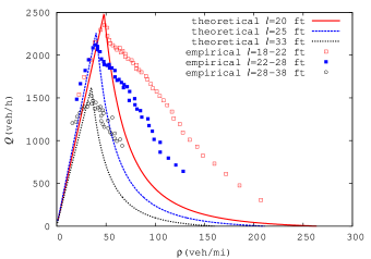
Figure 2: The flow-density relation: the lines represent the theoretical predictions derived from the non-local Prigogine-Herman kinetic equation for a gamma distribution, while the dots represent the traffic data measured by Coifman [21]. We have used the following parameters: $\alpha=120$, $\tau_{0}=35~{}s$, $\ell_{1}=33~{}ft$, $\ell_{2}=20~{}ft$ and $\epsilon\approx 1.12$. The correspondence between $\sigma-l$ is as follows: ($1.0~{}$-$~{}33ft$), ($0.38~{}$-$~{}25ft$) and ($0.0~{}$-$~{}20ft$).

At figure 3 the dependence of $z_{c}$ with $\sigma$ and $e=\ell_{2}/\ell_{1}$ for two different values of $\epsilon$. The parameter $e$ is a measure of the disparity of the lengths $\ell_{i}~{}(i=1,2)$, $e$ approaches to unity as $\ell_{2}\rightarrow\ell_{1}$ and approaches to zero as $\ell_{2}\rightarrow 0$ for $\ell_{1}$ fixed. In general, the critical value $z_{c}$ may remain fixed as $e$ increases and $\sigma$ decreases.

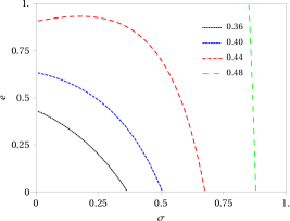
Figure 3: Contour levels at constant $z_{c}$ as a function of $\sigma$ and $e=\ell_{1}/\ell_{2}$ and for two different values $\varepsilon=2$ (left) and $\varepsilon=3/2$ (right).

5 Concluding Remarks

In this work, a theoretical model for multiclass traffic based on the Prigogine-Herman-Boltzmann equation [19] has been determined. It has been shown that the fundamental diagram, as well as other important quantities such as the critical density and the road capacity can be derived from a theoretical model. The flux-density relation has been solved numerically from our model, and the obtained diagram matches experimental data collected by Coifman in the individual regime for different values of the effective length $l$. However, we have noted that at moderate densities vehicles cannot be regarded as point-like objects, in fact they require a finite space for its own extension and reaction. In this sense it is necessary to incorporate some modifications to the PHB traffic equation, this aspects will be addressed in a near future.

acknowledgments

The authors acknowledge support from CONACyT through grant number CB2015/251273.

References

- [1] B. D. Greenshields. A study of traffic capacity. In D. C. Highway Research Board, Washington, editor, Proceedings of the Highway Research Board, pages 448–477, 1935.
- [2] B. S. Kerner. The Physics of Traffic Flow. Understanding Complex Systems. Springer, 2004.
- [3] M. Treiber, A. Kesting, and D. Helbing. Three-phase traffic theory and two-phase models with a fundamental diagram in the light of empirical stylized facts. Transp. Res. Part B, 44:983–1000, 2010. DOI: 10.1016/j.trb.2010.03.004.
- [4] B. S. Kerner. Introduction to Modern Traffic Flow Theory and Control. Springer, 2009.
- [5] D. Helbing. Traffic and related self-driven many-particle systems. Rev. Mod. Phys., 73(4):1067–1141, 2001.
- [6] F. van Wageningen-Kessels, H. van Lint, K. Vuik, and S. Hoogendoorn. Genealogy of traffic flow models. EURO J. Transp. Logist, pages 1–29, 2014. DOI: 10.1007/sl 3676-014-0045-5.
- [7] J. M. Del Castillo and F. G. Benítez. On the functional form of the speed density (i): general theory. Transp. Res. Part B, 29:373–389, 1995.
- [8] J. M. del Castillo. Three new models for the flow-density relationship: derivation and testing for freeway and urban data. Transportmetrica, 8(6):443–465, 2012. DOI: 10.1080/18128602.2011.556680.
- [9] H. M. Zhang. New perspectives on continuum traffic flow models. Netw. Spat. Econ., 1:9–33, 2001.
- [10] C. Buison and C. Ladier. Exploring the impact of homogeneity of traffic measurements on the existence of macroscopic fundamental diagrams. Transp. Res. Record: J. Transp. Res. Board, 2124:127–136, 2009. DOI: 10.3141/2124-12.
- [11] H. J. Cho and S. C. Lo. Modeling self-consistent multi-class dynamic traffic flow. Physica A, 312:342–362, 2002.
- [12] A. K. Gupta and V. K. Katiyar. A new multi-class continuum model for traffic flow. Transportmetrica, 3(1):73–85, 2007. DOI: 10.1080/18128600708685665.
- [13] S. P. Hoogendoorn and P. H. L. Bovy. Continuum modeling of multiclass traffic flow. Transp. Res. Part B, 34:123–146, 2000.
- [14] G. C. Wong and S. C. Wong. A multi-class traffic flow model – an extension of LWR model with heterogeneous drivers. Transp. Res. Part A, 36:827–841, 2001.
- [15] D. Ngoduy. Multiclass first-order modelling of traffic networks using discontinuous flow-density relationships. Transportmetrica, 6(2):121–141, 2010. DOI: 10.1080/18128600902857925.
- [16] D. Ngoduy. Multiclass first-order traffic model using stochastic fundamental diagrams. Transportmetrica, 7(2):111–125, 2011. DOI: 10.1080/18126009032251334.
- [17] van Wageningen-Kessels F., B. van’t Hof, S. P. Hoogerdoorn, H. van Lint, and K. Vuik. Anisotropy in genric multi-class traffic flow models. Transportmetrica A: Transp. Sci., 9(5):451–472, 2013. DOI: 10.1080/18128602.2011.596289.
- [18] P. Zhang, S. C. Wong, and C. W. Shu. A weighted essentially non-oscillatory numerical scheme for a multi-class traffic flow model on an inhomogeneous highway. J. Comput. Phys., 212:739–756, 2006. DOI: 10.1016/j.jcp.2005.07.019.
- [19] I. Prigogine and R. Herman. Kinetic Theory of Vehicular Traffic. Elsevier, 1971.
- [20] M. L. L. Iannini and R. Dickman. Kinetic theory of vehicular traffic. Am. J. Phys., 84(2):135–145, 2016. DOI: 10.1119/1.4935895.
- [21] B. Coifman. Empirical flow-density and speed-spacing relationships: Evidence of vehicle lenght dependence. Transp.Res. Part B, 78:54–65, 2015. DOI: 10.1016/j.trb.2015.04.006.