Single cut and multicut SDDP with cut selection for multistage stochastic linear programs: convergence proof and numerical experiments

Abstract.

We introduce a variant of Multicut Decomposition Algorithms (MuDA), called CuSMuDA (Cut Selection for Multicut Decomposition Algorithms), for solving multistage stochastic linear programs that incorporates a class of cut selection strategies to choose the most relevant cuts of the approximate recourse functions. This class contains Level 1 [28] and Limited Memory Level 1 [16] cut selection strategies, initially introduced for respectively Stochastic Dual Dynamic Programming (SDDP) and Dual Dynamic Programming (DDP). We prove the almost sure convergence of the method in a finite number of iterations and obtain as a by-product the almost sure convergence in a finite number of iterations of SDDP combined with our class of cut selection strategies.

We compare the performance of MuDA, SDDP, and their variants with cut selection (using Level 1 and Limited Memory Level 1) on several instances of a portfolio problem and of an inventory problem. On these experiments, in general, SDDP is quicker (i.e., satisfies the stopping criterion quicker) than MuDA and cut selection allows us to decrease the computational bulk with Limited Memory Level 1 being more efficient (sometimes much more) than Level 1.

Vincent Guigues (corresponding author) School of Applied Mathematics, FGV Praia de Botafogo, Rio de Janeiro, Brazil vguigues@fgv.br Michelle Bandarra School of Applied Mathematics, FGV Praia de Botafogo, Rio de Janeiro, Brazil michelle.bandarra@mirow.com.br

Keywords: Stochastic Programming; Stochastic Dual Dynamic Programming; Multicut Decomposition Algorithm; Portfolio selection; Inventory management.

AMS subject classifications: 90C15, 91B30.

1. Introduction

Multistage stochastic optimization problems are common in many areas of engineering and in finance. However, solving these problems is challenging and in general requires decomposition techniques. Two popular decomposition methods are Approximate Dynamic Programming (ADP) [30] and sampling-based variants of the Nested Decomposition (ND) algorithm [6, 5] and of the Multicut Nested Decomposition (MuND) algorithm [9, 11]. The introduction of sampling within ND was proposed by [25] and the corresponding method is usually called Stochastic Dual Dynamic Programming (SDDP). Several enhancements and extensions of SDDP have been proposed such as CUPPS [10], ReSA [20], AND [7], DOASA [29], risk-averse variants in [17, 18, 27, 14, 34, 22], cut formulas for nonlinear problems in [15], regularizations in [2] for linear problems and SDDP-REG in [19] for nonlinear problems. Convergence of these methods was proved in [29] for linear problems, in [13] for nonlinear risk-neutral problems, and in [15] for risk-averse nonlinear problems. All these algorithms compute lower approximations of the cost-to-go functions expressed as a supremum of affine functions called optimality cuts. Typically, at each iteration, a fixed number of cuts is added for each cost-to-go function. Therefore, techniques to reduce the number of cuts in each subproblem (referred to as cut selection or cut pruning) may be helpful to speed up the convergence of these methods. In stochastic optimization, the problem of cut selection for lower approximations of the cost-to-go functions associated to each node of the scenario tree was discussed for the first time in [31] where only the active cuts are selected. Pruning strategies of basis (quadratic) functions have been proposed in [12] and [24] for max-plus based approximation methods which, similarly to SDDP, approximate the cost-to-go functions of a nonlinear optimal control problem by a supremum of basis functions. More precisely, in [12], a fixed number of cuts is eliminated and cut selection is done solving a combinatorial optimization problem. For SDDP, in [34] it is suggested at some iterations to eliminate redundant cuts (a cut is redundant if it is never active in describing the lower approximate cost-to-go function). This procedure is called test of usefulness in [26]. This requires solving at each stage as many linear programs as there are cuts. In [26] and [28], only the cuts that have the largest value for at least one of the trial points computed are considered relevant. This strategy is called the Territory algorithm in [26] and Level 1 cut selection in [28]. It was presented for the first time in 2007 at the ROADEF congress by David Game and Guillaume Le Roy (GDF-Suez), see [26].

Sampling can also be incorporated into MuND algorithm (see for instance [36]). This algorithm builds many more cuts than SDDP per iteration and therefore each iteration takes more time but less iterations are in general needed to satisfy some stopping criterion. Therefore, cut selection strategies could also be useful. However, to the best of our knowledge, the combination of multicut decomposition methods with cut selection strategies, refereed to as CuSMuDA (Cut Selection for Multicut Decomposition Algorithms) in the sequel, has not been proposed so far. In this context, the objectives and contributions of this paper are the following:

• we propose cut selection strategies that are more efficient than the aforementioned ones. More precisely, instead of selecting all the cuts that are the highest at the trial points, we introduce a set of selectors that select some subset of these cuts. The selectors have to satisfy an assumption (Assumption (H3), see Section 3.2) to ensure the convergence of SDDP and MuDA combined with these cut selection strategies. We obtain a family of cut selection strategies; a given strategy corresponding to a choice of selectors along the iterations. In this family, the most economic (in terms of memory) cut selection strategy satisfying (H3) is the Limited Memory Level 1 (LML 1) strategy which selects at each trial point only one cut, namely the oldest cut. This strategy was introduced in [16] in the context of Dual Dynamic Programming but can be straightforwardly applied to SDDP and MuDA. The least economic strategy, i.e., the one that keeps the largest amount of cuts, is Level 1. “Between” these two strategies, using the flexibility offered by the selectors (as long as Assumption (H3) is satisfied by these selectors), we obtain a (large) family of cut selection strategies.

• We introduce and describe CuSMuDA, a combination of MuDA with our family of cut selection strategies.

• We prove the almost sure convergence of CuSMuDA in a finite number of iterations. This proof extends the theory in [16] in two aspects: (i) first the stochastic case is considered, i.e., SDDP and multicut SDDP are considered whereas the deterministic case, i.e., DDP, was considered in [16] and second (ii) more general cut selection strategies are dealt with. Item (ii) requires an additional technical discussion, see Lemma 1.

• We present the results of numerical experiments comparing the performance of six solution methods on several instances of a portfolio problem and of an inventory problem. These six solution methods are SDDP, SDDP with Level 1 cut selection, SDDP with LML 1 cut selection, MuDA, CuSMuDA with Level 1 cut selection, and CuSMuDA with LML 1 cut selection. To the best of our knowledge, these are the first numerical experiments on SDDP with LML 1 cut selection and the first experiments on multicut SDDP combined with cut selection. The main conclusions of these experiments are the following:

  • in general, for a given instance, CuSMuDA with LML 1 cut selection (resp. SDDP combined with LML 1 cut selection) is more efficient (i.e., allows us to satisfy more quickly the stopping criterion) than CuSMuDA with Level 1 cut selection (resp. SDDP combined with Level 1 cut selection), itself much more efficient than MuDA (resp. SDDP). Typically, variants with cut selection require more iterations but iterations are quicker with very few cuts selected for the first stages. However, on some instances, CuSMuDA with Level 1 cut selection still selected a large proportion of cuts for all stages and was less efficient than both MuDA and CuSMuDA with LML 1 cut selection.

  • MuDA (resp. CuSMuDA) in general requires much more computational bulk than SDDP (resp. SDDP with cut selection). However, on some instances, CuSMuDA with LML 1 cut selection and SDDP combined with LML 1 cut selection have shown similar performances. We also expect CuSMuDA to be more efficient than SDDP with cut selection when MuDA is already more efficient than SDDP. Even if this is not often the case, the results of numerical experiments on several instances of multistage stochastic linear programs where MuDA is quicker than SDDP are reported in [8].

The outline of the study is as follows. The class of problems considered and assumptions are discussed in Section 2. In Subsection 3.1 we recall sampling-based MuND while in Subsection 3.2 CuSMuDA is described. In Section 4, we prove Theorem 1 which states that CuSMuDA converges almost surely in a finite number of iterations to an optimal policy. As a by-product, we obtain the almost sure convergence of SDDP combined with our class of cut selection strategies (in particular Level 1 and LML 1) in a finite number of iterations. Finally, numerical experiments are presented in Section 5.

Throughout the paper, the usual scalar product in $\mathbb{R}^{n}$ is denoted by $\langle x,y\rangle=x^{\top}y$ for $x,y\in\mathbb{R}^{n}$.

2. Problem formulation and assumptions

We are interested in solution methods for linear stochastic dynamic programming equations: the first stage problem is

(1) $$\mathcal{Q}_{1}(x_{0})=\left\{\begin{array}[]{l}\inf_{x_{1}\in\mathbb{R}^{n}}\langle c_{1},x_{1}\rangle+\mathcal{Q}_{2}(x_{1})\\ A_{1}x_{1}+B_{1}x_{0}=b_{1},x_{1}\geq 0\end{array}\right.$$

for $x_{0}$ given and for $t=2,\ldots,T$, $\mathcal{Q}_{t}(x_{t-1})=\mathbb{E}_{\xi_{t}}[\mathfrak{Q}_{t}(x_{t-1},\xi_{t})]$ with

(2) $$\mathfrak{Q}_{t}(x_{t-1},\xi_{t})=\left\{\begin{array}[]{l}\inf_{x_{t}\in\mathbb{R}^{n}}\langle c_{t},x_{t}\rangle+\mathcal{Q}_{t+1}(x_{t})\\ A_{t}x_{t}+B_{t}x_{t-1}=b_{t},x_{t}\geq 0,\end{array}\right.$$

with the convention that $\mathcal{Q}_{T+1}$ is null and where for $t=2,\ldots,T$, random vector $\xi_{t}$ corresponds to the concatenation of the elements in random matrices $A_{t},B_{t}$ which have a known finite number of rows and random vectors $b_{t},c_{t}$ (it is assumed that $\xi_{1}$ is not random). For convenience, we will denote

$$X_{t}(x_{t-1},\xi_{t}):=\{x_{t}\in\mathbb{R}^{n}:A_{t}x_{t}+B_{t}x_{t-1}=b_{t},\,x_{t}\geq 0\}.$$

We make the following assumptions:

• The random vectors $\xi_{2},\ldots,\xi_{T}$ are independent and have discrete distributions with finite support.

• The set $X_{1}(x_{0},\xi_{1})$ is nonempty and bounded and for every $x_{1}\in X_{1}(x_{0},\xi_{1})$, for every $t=2,\ldots,T$, for every realization $\tilde{\xi}_{2},\ldots,\tilde{\xi}_{t}$ of $\xi_{2},\ldots,\xi_{t}$, for every $x_{\tau}\in X_{\tau}(x_{\tau-1},\tilde{\xi}_{\tau}),\tau=2,\ldots,t-1$, the set $X_{t}(x_{t-1},{\tilde{\xi}}_{t})$ is nonempty and bounded.

We will denote by $\Theta_{t}=\{\xi_{t1},\ldots,\xi_{tM_{t}}\}$ the support of $\xi_{t}$ for stage $t$ with $p_{ti}=\mathbb{P}(\xi_{t}=\xi_{ti})>0,i=1,\ldots,M_{t}$ and with vector $\xi_{tj}$ being the concatenation of the elements in $A_{tj},B_{tj},b_{tj},c_{tj}$.

3. Algorithms

3.1. Multicut stochastic decomposition

The multicut stochastic decomposition method approximates the function $\mathfrak{Q}_{t}(\cdot,\xi_{tj})$ at iteration $k$ for $t=2,\ldots,T$, $j=1,\ldots,M_{t}$, by a piecewise affine lower bounding function $\mathfrak{Q}_{t}^{k}(\cdot,\xi_{tj})$ which is a maximum of $k$ affine functions $\mathcal{C}_{tj}^{i}$ called cuts:

$$\mathfrak{Q}_{t}^{k}(x_{t-1},\xi_{tj})=\max_{1\leq i\leq k}\mathcal{C}_{tj}^{i}(x_{t-1})\mbox{ with }\mathcal{C}_{tj}^{i}(x_{t-1})=\theta_{tj}^{i}+\langle\beta_{tj}^{i},x_{t-1}\rangle$$

where coefficients $\theta_{tj}^{i},\beta_{tj}^{i}$ are computed as explained below. These approximations provide the lower bounding functions

(3) $$\mathcal{Q}_{t}^{k}(x_{t-1})=\sum_{j=1}^{M_{t}}p_{tj}\mathfrak{Q}_{t}^{k}(x_{t-1},\xi_{tj})$$

for $\mathcal{Q}_{t}$. Since $\mathcal{Q}_{T+1}$ is the null function, we will also define $\mathcal{Q}_{T+1}^{k}\equiv 0$. The steps of MuDA are described below.

Step 1: Initialization. For $t=2,\ldots,T$, $j=1,\ldots,M_{t}$, take for $\mathfrak{Q}_{t}^{0}(\cdot,\xi_{tj})$ a known lower bounding affine function for $\mathfrak{Q}_{t}(\cdot,\xi_{tj})$. Set the iteration count $k$ to 1 and $\mathcal{Q}_{T+1}^{0}\equiv 0$.

Step 2: Forward pass. We generate a sample ${\tilde{\xi}}^{k}=(\tilde{\xi}_{1}^{k},\tilde{\xi}_{2}^{k},\ldots,\tilde{\xi}_{T}^{k})$ from the distribution of $(\xi_{1},\xi_{2},\ldots,\xi_{T})$, with the convention that $\tilde{\xi}_{1}^{k}=\xi_{1}$ (here and in what follows, the tilde symbol will be used to represent realizations of random variables: for random variable $\xi$, $\tilde{\xi}$ is a realization of $\xi$). Using approximation $\mathfrak{Q}_{t}^{k-1}(\cdot,\xi_{tj})$ of $\mathfrak{Q}_{t}(\cdot,\xi_{tj})$ (computed at previous iterations), we solve the problem

(4) $$\left\{\begin{array}[]{l}\inf_{x_{t}\in\mathbb{R}^{n}}\langle x_{t},{\tilde{c}}_{t}^{k}\rangle+\mathcal{Q}_{t+1}^{k-1}(x_{t})\\ x_{t}\in X_{t}(x_{t-1}^{k},{\tilde{\xi}}_{t}^{k})\end{array}\right.$$

for $t=1,\ldots,T$, where $x_{0}^{k}=x_{0}$ and $\mathcal{Q}_{t+1}^{k-1}$ is given by (3) with $k$ replaced by $k-1$. Let $x_{t}^{k}$ be an optimal solution of the problem.

Step 3: Backward pass. The backward pass builds cuts for $\mathfrak{Q}_{t}(\cdot,\xi_{tj})$ at $x_{t-1}^{k}$ computed in the forward pass. For $k\geq 1$ and $t=1,\ldots,T$, we introduce the function ${\underline{\mathfrak{Q}}}_{t}^{k}:\mathbb{R}^{n}{\small{\times}}\Theta_{t}\rightarrow\mathbb{R}$ given by

(5) $${\underline{\mathfrak{Q}}}_{t}^{k}(x_{t-1},\xi_{t})=\left\{\begin{array}[]{l}\inf_{x_{t}\in\mathbb{R}^{n}}\langle c_{t},x_{t}\rangle+\mathcal{Q}_{t+1}^{k}(x_{t})\\ x_{t}\in X_{t}(x_{t-1},\xi_{t}),\end{array}\right.$$

with the convention that $\Theta_{1}=\{\xi_{1}\}$, and we set $\mathcal{Q}_{T+1}^{k}\equiv 0$. For $j=1,\ldots,M_{T}$, we solve the problem

(6) $$\mathfrak{Q}_{T}(x_{T-1}^{k},\xi_{Tj})=\left\{\begin{array}[]{l}\displaystyle\inf_{x_{T}\in\mathbb{R}^{n}}\langle c_{Tj},x_{T}\rangle\\ A_{Tj}x_{T}+B_{Tj}x_{T-1}^{k}=b_{Tj},x_{T}\geq 0,\end{array}\right.\mbox{ with dual }\left\{\begin{array}[]{l}\sup_{\lambda}\langle\lambda,b_{Tj}-B_{Tj}x_{T-1}^{k}\rangle\\ A_{Tj}^{\top}\lambda\leq c_{Tj}.\end{array}\right.$$

Let $\lambda_{Tj}^{k}$ be an optimal solution of the dual problem above. We get

$$\mathfrak{Q}_{T}(x_{T-1},\xi_{Tj})\geq\langle\lambda_{Tj}^{k},b_{Tj}-B_{Tj}x_{T-1}\rangle$$

and compute $\theta_{Tj}^{k}=\langle b_{Tj},\lambda_{Tj}^{k}\rangle$ and $\beta_{Tj}^{k}=-B_{Tj}^{\top}\lambda_{Tj}^{k}$. Then for $t=T-1$ down to $t=2$, knowing $\mathcal{Q}_{t+1}^{k}\leq\mathcal{Q}_{t+1}$, we solve the problem below for $j=1,\ldots,M_{t}$,

(7) $${\underline{\mathfrak{Q}}}_{t}^{k}(x_{t-1}^{k},\xi_{tj})=\left\{\begin{array}[]{l}\displaystyle\inf_{x_{t}}\langle c_{tj},x_{t}\rangle+\mathcal{Q}_{t+1}^{k}(x_{t})\\ x_{t}\in X_{t}(x_{t-1}^{k},\xi_{tj})\end{array}\right.=\left\{\begin{array}[]{l}\displaystyle\inf_{x_{t},f}\langle c_{tj},x_{t}\rangle+\sum_{\ell=1}^{M_{t+1}}p_{t+1\ell}f_{\ell}\\ A_{tj}x_{t}+B_{tj}x_{t-1}^{k}=b_{tj},x_{t}\geq 0,\\ f_{\ell}\geq\theta_{t+1\ell}^{i}+\langle\beta_{t+1\ell}^{i},x_{t}\rangle,i=1,\ldots,k,\ell=1,\ldots,M_{t+1}.\end{array}\right.$$

Observe that due to (H2) the above problem is feasible and has a finite optimal value. Therefore ${\underline{\mathfrak{Q}}}_{t}^{k}(x_{t-1}^{k},\xi_{tj})$ can be expressed as the optimal value of the corresponding dual problem:

(8) $${\underline{\mathfrak{Q}}}_{t}^{k}(x_{t-1}^{k},\xi_{tj})=\left\{\begin{array}[]{l}\displaystyle\sup_{\lambda,\mu}\;\langle\lambda,b_{tj}-B_{tj}x_{t-1}^{k}\rangle+\sum_{i=1}^{k}\sum_{\ell=1}^{M_{t+1}}\mu_{i\ell}\theta_{t+1\ell}^{i}\\ A_{tj}^{\top}\lambda+\sum_{i=1}^{k}\sum_{\ell=1}^{M_{t+1}}\mu_{i\ell}\beta_{t+1\ell}^{i}\leq c_{tj},\\ p_{t+1\ell}=\sum_{i=1}^{k}\mu_{i\ell},\,\ell=1,\ldots,M_{t+1},\\ \mu_{i\ell}\geq 0,\,i=1,\ldots,k,\ell=1,\ldots,M_{t+1}.\end{array}\right.$$

Let $(\lambda_{tj}^{k},\mu_{tj}^{k})$ be an optimal solution of dual problem (8). Using the fact that $\mathcal{Q}_{t+1}^{k}\leq\mathcal{Q}_{t+1}$, we get

$$\mathfrak{Q}_{t}(x_{t-1},\xi_{tj})\geq{\underline{\mathfrak{Q}}}_{t}^{k}(x_{t-1},\xi_{tj})\geq\langle\lambda_{tj}^{k},b_{tj}-B_{tj}x_{t-1}\rangle+\langle\mu_{tj}^{k},\theta_{t+1}^{k}\rangle$$

and we compute

$$\theta_{tj}^{k}=\langle\lambda_{tj}^{k},b_{tj}\rangle+\langle\mu_{tj}^{k},\theta_{t+1}^{k}\rangle\mbox{ and }\beta_{tj}^{k}=-B_{tj}^{\top}\lambda_{tj}^{k}.$$

In these expressions, vector $\theta_{t+1}^{k}$ has components $\theta_{t+1\ell}^{i},\ell=1,\ldots,M_{t+1},i=1,\ldots,k$, arranged in the same order as components $\mu_{tj}^{k}(\ell,i)$ of $\mu_{tj}^{k}$.

Step 4: Do $k\leftarrow k+1$ and go to Step 2.

3.2. Multicut stochastic decomposition with cut selection

We now describe a variant of MuDA that stores all cut coefficients $\theta_{tj}^{i},\beta_{tj}^{i}$, and trial points $x_{t-1}^{i}$, but that uses a reduced set of cuts $\mathcal{C}_{tj}^{i}$ to approximate functions $\mathfrak{Q}_{t}(\cdot,\xi_{tj})$ when solving problem (4) in the forward pass and (7) in the backward pass. Let $S_{tj}^{k}$ be the set of indices of the cuts selected at the end of iteration $k$ to approximate $\mathfrak{Q}_{t}(\cdot,\xi_{tj})$. At the end of the backward pass of iteration $k$, the variant of MuDA with cut selection computes approximations $\mathcal{Q}_{t}^{k}$ of $\mathcal{Q}_{t}$ given by (3) now with $\mathfrak{Q}_{t}^{k}(\cdot,\xi_{tj})$ given by

(9) $$\mathfrak{Q}_{t}^{k}(x_{t-1},\xi_{tj})=\max_{\ell\in S_{tj}^{k}}\,\mathcal{C}_{tj}^{\ell}(x_{t-1}),$$

where the set $S_{tj}^{k}$ is a subset of the set of indices of the cuts that have the largest value for at least one of the trial points computed so far. More precisely, sets $S_{tj}^{k}$ are initialized taking $S_{tj}^{0}=\{0\}$. For $t\in\{2,\ldots,T\}$ and $k\geq 1$, sets $S_{tj}^{k}$ are computed as follows. For $i=1,\ldots,k$, $t=2,\ldots,T$, $j=1,\ldots,M_{t}$, let $I_{tj}^{ik}$ be the set of cuts for $\mathfrak{Q}_{t}(\cdot,\xi_{tj})$ computed at iteration $k$ or before, that have the largest value at $x_{t-1}^{i}$:

(10) $$I_{tj}^{ik}=\operatorname*{arg\,max}_{\ell=1,\ldots,k}\mathcal{C}_{tj}^{\ell}(x_{t-1}^{i}),$$

where the cut indices in $I_{tj}^{ik}$ are sorted in ascending order. With a slight abuse of notation, we will denote the $\ell$-th smallest element in $I_{tj}^{ik}$ by $I_{tj}^{ik}(\ell)$. For instance, if $I_{tj}^{ik}=\{2,30,50\}$ then $I_{tj}^{ik}(1)=2,I_{tj}^{ik}(2)=30$, and $I_{tj}^{ik}(3)=50$. A cut selection strategy is given by a set of selectors $\mathcal{S}_{tj}(m)$, $t=2,\ldots,T$,$j=1,\ldots,M_{t}$, $m=1,2,\ldots,$ where $\mathcal{S}_{tj}(m)$ is a subset of the set of $m$ integers $\{1,2,\ldots,m\}$, giving the indices of the cuts to select in $I_{tj}^{ik}$ through the relation

$$S_{tj}^{k}=\bigcup_{i=1}^{k}\left\{I_{tj}^{ik}(\ell):\ell\in\mathcal{S}_{tj}(|I_{tj}^{ik}|)\right\},$$

where $|I_{tj}^{ik}|$ is the cardinality of set $I_{tj}^{ik}$. We require the selectors to satisfy the following assumption:

• for $t=2,\ldots,T$, $j=1,\ldots,M_{t}$, for every $m\geq 1$, $\mathcal{S}_{tj}(m)\subseteq\mathcal{S}_{tj}(m+1)$.

Level 1 and Limited Memory Level 1 cut selection strategies described in Examples 3.1 and 3.2 respectively correspond to the least and most economic selectors satisfying (H3):

Example 3.1 (Level 1 and Territory Algorithm).

The strategy $\mathcal{S}_{tj}(m)=\{1,2,\ldots,m\}$ selects all cuts that have the highest value for at least one trial point. In the context of SDDP, this strategy was called Level 1 in [28] and Territory Algorithm in [26]. For this strategy, we have $S_{Tj}^{k}=\{1,\ldots,k\}$ for all $j$ and $k\geq 1$, meaning that no cut selection is needed for the last stage $T$. This comes from the fact that for all $k\geq 2$ and $1\leq k_{1}\leq k$, cut $\mathcal{C}_{Tj}^{k_{1}}$ is selected because it is one of the cuts with the highest value at $x_{T-1}^{k_{1}}$. Indeed, for any $1\leq k_{2}\leq k$ with $k_{2}\neq k_{1}$, since $\lambda_{Tj}^{k_{2}}$ is feasible for problem (6) with $x_{T-1}^{k}$ replaced by $x_{T-1}^{k_{1}}$, we get

$$\mathcal{C}_{Tj}^{k_{1}}(x_{T-1}^{k_{1}})=\mathfrak{Q}_{T}(x_{T-1}^{k_{1}},\xi_{Tj})\geq\langle\lambda_{Tj}^{k_{2}},b_{Tj}-B_{Tj}x_{T-1}^{k_{1}}\rangle=\mathcal{C}_{Tj}^{k_{2}}(x_{T-1}^{k_{1}}).$$

Example 3.2 (Limited Memory Level 1).

The strategy that eliminates the largest amount of cuts, called Limited Memory Level 1 (LML 1 for short), consists in taking a singleton for every set $\mathcal{S}_{tj}(m)$. For (H3) to be satisfied, this implies $\mathcal{S}_{tj}(m)=\{1\}$. This choice corresponds to the Limited Memory Level 1 cut selection introduced in [16] in the context of DDP. For that particular choice, at a given point, among the cuts that have the highest value only the oldest (i.e., the cut that was first computed among the cuts that have the highest value at that point) is selected.

Remark 3.1.

Observe that our selectors select cuts for functions $\mathfrak{Q}_{t}(\cdot,\xi_{tj})$ whereas Level 1 (resp. LML 1) was introduced to select cuts for functions $\mathcal{Q}_{t}$ for SDDP (resp. DDP). Therefore we could have used the terminologies Multicut Level 1 and Multicut Limited Memory Level 1 instead of Level 1 and Limited Memory Level 1. We did not do so to simplify and therefore to know to which functions cut selection strategies apply, it suffices to add the name of the decomposition method; for instance MuDA with Level 1 cut selection (in which case cut selection applies to functions $\mathfrak{Q}_{t}(\cdot,\xi_{tj})$, as explained above) or SDDP with Limited Memory Level 1 cut selection (in which case cut selection applies to functions $\mathcal{Q}_{t}$).

The computation of $S_{tj}^{k}$, i.e., of the cut indices to select at iteration $k$, is performed in the backward pass (immediately after computing cut $\mathcal{C}_{tj}^{k}$) using the pseudo-code given in the left and right panels of Figure 1 for the Level 1 and LML 1 cut selection strategies respectively.

In this pseudo-code, we use the notation $I_{tj}^{i}$ in place of $I_{tj}^{ik}$. We also store in variable $m_{tj}^{i}$ the current value of the highest cut for $\mathfrak{Q}_{t}(\cdot,\xi_{tj})$ at $x_{t-1}^{i}$. At the end of the first iteration, we initialize $m_{tj}^{1}=\mathcal{C}_{tj}^{1}(x_{t-1}^{1})$. After cut $\mathcal{C}_{tj}^{k}$ is computed at iteration $k\geq 2$, these variables are updated using the relations

$$\left\{\begin{array}[]{lll}m_{tj}^{i}&\leftarrow&\max(m_{tj}^{i},\mathcal{C}_{tj}^{k}(x_{t-1}^{i})),\;i=1,\ldots,k-1,\\ m_{tj}^{k}&\leftarrow&\max(\mathcal{C}_{tj}^{\ell}(x_{t-1}^{k}),\ell=1,\ldots,k).\end{array}\right.$$

We also use an array of Boolean called Selected using the information given by variables $I_{tj}^{i}$ whose $\ell$-th entry is True if cut $\ell$ is selected for $\mathfrak{Q}_{t}(\cdot,\xi_{tj})$ and False otherwise. This allows us to avoid copies of cut indices that may appear in $I_{t{j}}^{i_{1}k}$ and $I_{t{j}}^{i_{2}k}$ with $i_{1}\neq i_{2}$.

Level 1

Limited Memory Level 1

$I_{tj}^{k}=\{k\}$, $m_{tj}^{k}=\mathcal{C}_{tj}^{k}(x_{t-1}^{k})$. For $\ell=1,\ldots,k-1$, If $\mathcal{C}_{tj}^{k}(x_{t-1}^{\ell})>m_{tj}^{\ell}$         $I_{tj}^{\ell}=\{k\},\;m_{tj}^{\ell}=\mathcal{C}_{tj}^{k}(x_{t-1}^{\ell})$ Else if $\mathcal{C}_{tj}^{k}(x_{t-1}^{\ell})=m_{tj}^{\ell}$         $I_{tj}^{\ell}=I_{tj}^{\ell}\cup\{k\}$ End If If $\mathcal{C}_{tj}^{\ell}(x_{t-1}^{k})>m_{tj}^{k}$         $I_{tj}^{k}=\{\ell\},\;m_{tj}^{k}=\mathcal{C}_{tj}^{\ell}(x_{t-1}^{k})$ Else if $\mathcal{C}_{tj}^{\ell}(x_{t-1}^{k})=m_{tj}^{k}$         $I_{tj}^{k}=I_{tj}^{k}\cup\{\ell\}$ End If End For For $\ell=1,\ldots,k$, Selected[$\ell$]=False End For For $\ell=1,\ldots,k$ For $m=1,\ldots,|I_{tj}^{\ell}|$         Selected[$I_{tj}^{\ell}[m]$]=True End For End For $S_{tj}^{k}=\emptyset$ For $\ell=1,\ldots,k$ If Selected[$\ell$]=True         $S_{tj}^{k}=S_{tj}^{k}\cup\{\ell\}$ End If End For

$I_{tj}^{k}=\{1\}$, $m_{tj}^{k}=\mathcal{C}_{tj}^{1}(x_{t-1}^{k})$. For $\ell=1,\ldots,k-1$, If $\mathcal{C}_{tj}^{k}(x_{t-1}^{\ell})>m_{tj}^{\ell}$         $I_{tj}^{\ell}=\{k\},\;m_{tj}^{\ell}=\mathcal{C}_{tj}^{k}(x_{t-1}^{\ell})$ End If If $\mathcal{C}_{tj}^{\ell+1}(x_{t-1}^{k})>m_{tj}^{k}$         $I_{tj}^{k}=\{\ell+1\},\;m_{tj}^{k}=\mathcal{C}_{tj}^{\ell+1}(x_{t-1}^{k})$ End If End For For $\ell=1,\ldots,k$, Selected[$\ell$]=False End For For $\ell=1,\ldots,k$ For $m=1,\ldots,|I_{tj}^{\ell}|$         Selected[$I_{tj}^{\ell}[m]$]=True End For End For $S_{tj}^{k}=\emptyset$ For $\ell=1,\ldots,k$ If Selected[$\ell$]=True         $S_{tj}^{k}=S_{tj}^{k}\cup\{\ell\}$ End If End For

Figure 1. Pseudo-codes for the computation of set $S_{tj}^{k}$ for fixed $t\in\{2,\ldots,T\},k\geq 2,j=1,\ldots,M_{t}$, and two cut selection strategies.

4. Convergence analysis

In this section, we prove that CuSMuDA converges in a finite number of iterations. We will make the following assumption:

• The samples in the forward passes are independent: $(\tilde{\xi}_{2}^{k},\ldots,\tilde{\xi}_{T}^{k})$ is a realization of $\xi^{k}=(\xi_{2}^{k},\ldots,\xi_{T}^{k})\sim(\xi_{2},\ldots,\xi_{T})$ and $\xi^{1},\xi^{2},\ldots,$ are independent.

The convergence proof is based on the following lemma:

Lemma 1.

Assume that all subproblems in the forward and backward passes of CuSMuDA are solved using an algorithm that necessarily outputs an extreme point of the feasible set (for instance the simplex algorithm). Let assumptions (H1), (H2), (H3), and (H4) hold. Then almost surely, there exists $k_{0}\geq 1$ such that for every $k\geq k_{0}$, $t=2,\ldots,T$, $j=1,\ldots,M_{t}$, we have

(11) $$\mathfrak{Q}_{t}^{k}(\cdot,\xi_{tj})=\mathfrak{Q}_{t}^{k_{0}}(\cdot,\xi_{tj})\mbox{ and }\mathcal{Q}_{t}^{k}=\mathcal{Q}_{t}^{k_{0}}.$$

Proof.

Let $\Omega_{1}$ be the event on the sample space $\Omega$ of sequences of forward scenarios such that every scenario is sampled an infinite number of times. By Assumption (H4), this event $\Omega_{1}$ has probability one.

Consider a realization $\omega\in\Omega$ of CuSMuDA in $\Omega_{1}$ corresponding to realizations $(\tilde{\xi}^{k}_{1:T})_{k}$ of $(\xi^{k}_{1:T})_{k}$ in the forward pass. To simplify, we will drop $\omega$ in the notation. For instance, we will simply write $x_{t}^{k},\mathcal{Q}_{t}^{k}$ for realizations $x_{t}^{k}(\omega)$ and $\mathcal{Q}_{t}^{k}(\cdot)(\omega)$ of $x_{t}^{k},\mathcal{Q}_{t}^{k}$ given realization $\omega\in\Omega$ of CuSMuDA.

We show by induction on $t$ that the number of different cuts computed by the algorithm is finite and that after some iteration $k_{t}$ the same cuts are selected for functions $\mathfrak{Q}_{t}(\cdot,\xi_{tj})$. Our induction hypothesis $\mathcal{H}(t)$ for $t\in\{2,\ldots,T\}$ is that the sets $\{(\theta_{tj}^{k},\beta_{tj}^{k}):k\in\mathbb{N}\},j=1,\ldots,M_{t}$, are finite and there exists some finite $k_{t}$ such that for every $k>k_{t}$ we have

(12) $$\{(\theta_{tj}^{\ell},\beta_{tj}^{\ell}):\ell\in S_{tj}^{k}\}=\{(\theta_{tj}^{\ell},\beta_{tj}^{\ell}):\ell\in S_{tj}^{k_{t}}\}\mbox{ and }x_{t-1}^{k}=x_{t-1}^{k_{t}},$$

for every $j=1,\ldots,M_{t}$. We will denote by $\mathcal{I}_{tj}^{ik}$ the set $\left\{I_{tj}^{ik}(\ell):\ell\in\mathcal{S}_{tj}(|I_{tj}^{ik}|)\right\}$. We first show, in items a and b below that $\mathcal{H}(T)$ holds.

a. Observe that $\lambda_{Tj}^{k}$ defined in the backward pass of CuSMuDA is an extreme point of the polyhedron $\{\lambda:A_{Tj}^{\top}\lambda\leq c_{Tj}\}$. This polyhedron is a finite intersection of closed half spaces in finite dimension (since $A_{Tj}$ has a finite number of rows and columns) and therefore has a finite number of extreme points. It follows that $\lambda_{Tj}^{k}$ can only take a finite number of values, same as $(\theta_{Tj}^{k},\beta_{Tj}^{k})=(\langle\lambda_{Tj}^{k},b_{Tj}\rangle,-B_{Tj}^{\top}\lambda_{Tj}^{k})$, and there exists ${\bar{k}}_{T}$ such that for every $k>{\bar{k}}_{T}$ and every $j$, each cut $\mathcal{C}_{Tj}^{k}$ is a copy of a cut $\mathcal{C}_{Tj}^{k^{\prime}}$ with $1\leq k^{\prime}\leq{\bar{k}}_{T}$ (no new cut is computed for functions $\mathfrak{Q}_{T}(\cdot,\xi_{Tj})$ for $k>{\bar{k}}_{T}$).

Now recall that $x_{T-1}^{k}$ computed in the forward pass is a solution of (4) with $t=T-1$ and this optimization problem can be written as a linear problem adding variables $f_{1},f_{2},\ldots,f_{M_{T}}$ replacing in the objective $\mathcal{Q}_{T}^{k-1}(x_{T-1})$ by $\sum_{\ell=1}^{M_{T}}p_{T\ell}f_{\ell}$ and adding the linear constraints $f_{\ell}\geq\theta_{T\ell}^{i}+\langle\beta_{T\ell}^{i},x_{T-1}\rangle$, $i=1,\ldots,k-1,$ $\ell=1,\ldots,M_{T}$. On top of that, for iterations $k>{\bar{k}}_{T}$, since functions $\mathfrak{Q}_{T}^{k}(\cdot,\xi_{Tj})$ are made of a collection of cuts taken from the finite and fixed set of cuts $\mathcal{C}_{Tj}^{\ell},\ell\leq\bar{k}_{T}$, the set of possible functions $(\mathfrak{Q}_{T}^{k}(\cdot,\xi_{Tj}))_{k\geq 1}$ and therefore of possible functions $(\mathcal{Q}_{T}^{k})_{k\geq 1}$ is finite. It follows that there is a finite set of possible polyhedrons for the feasible set of (4) (with $t=T-1$) rewritten as a linear program as we have just explained, adding variables $f_{1},f_{2},\ldots,f_{M_{T}}$. Since these polyhedrons have a finite number of extreme points (recall that there is a finite number of different linear constraints), there is only a finite number of possible trial points $(x_{T-1}^{k})_{k\geq 1}$. Therefore we can assume without loss of generality that $\bar{k}_{T}$ is such that for iterations $k>\bar{k}_{T}$, all trial point $x_{T-1}^{k}$ is also a copy of a trial point $x_{T-1}^{k^{\prime}}$ with $k^{\prime}\leq\bar{k}_{T}$.

b. We show that for every $i\geq 1$ and $j=1,\ldots,M_{T}$, there exists $1\leq i^{\prime}\leq{\bar{k}}_{T}$ and $k_{Tj}(i^{\prime})\geq{\bar{k}}_{T}$ such that for every $k\geq\max(i,k_{Tj}(i^{\prime}))$ we have

(13) $$\left\{(\theta_{Tj}^{\ell},\beta_{Tj}^{\ell}):\ell\in\mathcal{I}_{Tj}^{ik}\right\}=\left\{(\theta_{Tj}^{\ell},\beta_{Tj}^{\ell}):\ell\in\mathcal{I}_{Tj}^{i^{\prime}k_{Tj}(i^{\prime})}\right\},$$

which will show $\mathcal{H}(T)$ with $k_{T}=\max_{1\leq j\leq M_{T},1\leq i^{\prime}\leq{\bar{k}}_{T}}k_{Tj}(i^{\prime})$. Let us show that (13) indeed holds. Let us take $i\geq 1$ and $j\in\{1,\ldots,M_{T}\}$. If $1\leq i\leq{\bar{k}}_{T}$ define $i^{\prime}=i$. Otherwise due to a. we can find $1\leq i^{\prime}\leq{\bar{k}}_{T}$ such that $x_{T-1}^{i}=x_{T-1}^{i^{\prime}}$ which implies $I_{Tj}^{ik}=I_{Tj}^{i^{\prime}k}$ for every $k\geq i$. Now consider the sequence of sets $(I_{Tj}^{i^{\prime}k})_{k\geq{\bar{k}}_{T}}$. Due to the definition of $\bar{k}_{T}$, the sequence $(|I_{Tj}^{i^{\prime}k}|)_{k>{\bar{k}}_{T}}$ is nondecreasing and therefore two cases can happen:

• there exists $k_{Tj}(i^{\prime})$ such that for $k\geq k_{Tj}(i^{\prime})$ we have $I_{Tj}^{i^{\prime}k}=I_{Tj}^{i^{\prime}k_{Tj}(i^{\prime})}$ (the cuts computed after iteration $k_{Tj}(i^{\prime})$ are not active at $x_{T-1}^{i^{\prime}}$). In this case $\mathcal{I}_{Tj}^{i^{\prime}k}=\mathcal{I}_{Tj}^{i^{\prime}k_{Tj}(i^{\prime})}$ for $k\geq k_{Tj}(i^{\prime})$, $\mathcal{I}_{Tj}^{ik}=\mathcal{I}_{Tj}^{i^{\prime}k}=\mathcal{I}_{Tj}^{i^{\prime}k_{Tj}(i^{\prime})}$ for $k\geq\max(k_{Tj}(i^{\prime}),i)$ and (13) holds.

• The sequence $(|I_{Tj}^{i^{\prime}k}|)_{k\geq{\bar{k}}_{T}}$ is unbounded. Due to Assumption (H3), the sequence $(|\mathcal{S}_{Tj}(m)|)_{m}$ is nondecreasing. If there exists $k_{Tj}>\bar{k}_{T}$ such that $\mathcal{S}_{Tj}(k)=\mathcal{S}_{Tj}(k_{Tj})$ for $k\geq k_{Tj}$ then if $k_{Tj}(i^{\prime})$ is the smallest $k$ such that $|I_{Tj}^{i^{\prime}k}|\geq k_{Tj}$ then for every $k\geq k_{Tj}(i^{\prime})$ we have $\mathcal{I}_{Tj}^{i^{\prime}k}=\mathcal{I}_{Tj}^{i^{\prime}k_{Tj}(i^{\prime})}$ and for $k\geq\max(k_{Tj}(i^{\prime}),i)$ we deduce $\mathcal{I}_{Tj}^{ik}=\mathcal{I}_{Tj}^{i^{\prime}k_{Tj}(i^{\prime})}$ and (13) holds. Otherwise the sequence $(|\mathcal{S}_{Tj}(m)|)_{m}$ is unbounded and an infinite number of cut indices are selected from the sets $(I_{Tj}^{i^{\prime}k})_{k\geq i^{\prime}}$ to make up sets $(\mathcal{I}_{Tj}^{i^{\prime}k})_{k\geq i^{\prime}}$. However, since there is a finite number of different cuts, there is only a finite number of iterations where a new cut can be selected from $I_{Tj}^{i^{\prime}k}$ and therefore there exists $k_{Tj}(i^{\prime})$ such that (13) holds for $k\geq\max(k_{Tj}(i^{\prime}),i)$.

c.

Now assume that $\mathcal{H}(t+1)$ holds for some $t\in\{2,\ldots,T-1\}$. We want to show $\mathcal{H}(t)$. Consider the set $\mathcal{D}_{tjk}$ of points of form

(14) $$(\langle\lambda,b_{tj}\rangle+\sum_{\ell=1}^{M_{t+1}}\sum_{i\in S_{t+1\ell}^{k}}\mu_{i\ell}\theta_{t+1\ell}^{i},-B_{tj}^{\top}\lambda)$$

where $(\lambda,\mu)$ is an extreme point of the set $\mathcal{P}_{tjk}$ of points $(\lambda,\mu)$ satisfying

(15) $$\begin{array}[]{l}\mu\geq 0,p_{t+1\ell}=\sum_{i\in S_{t+1\ell}^{k}}\mu_{i\ell},\;\ell=1,\ldots,M_{t+1},\;A_{tj}^{\top}\lambda+\sum_{\ell=1}^{M_{t+1}}\sum_{i\in S_{t+1\ell}^{k}}\mu_{i\ell}\beta_{t+1\ell}^{i}\leq c_{tj}.\end{array}$$

We claim that for every $k>k_{t+1}$, every point from $\mathcal{D}_{tjk}$ can be written as a point from $\mathcal{D}_{tjk_{t+1}}$, i.e., a point of form (14) with $k$ replaced by $k_{t+1}$ and $(\lambda,\mu)$ an extreme point of the set $\mathcal{P}_{tjk_{t+1}}$. Indeed, take a point from $\mathcal{D}_{tjk}$, i.e., a point of form (14) with $(\lambda,\mu)$ an extreme point of $\mathcal{P}_{tjk}$ and $k>k_{t+1}$. It can be written as a point from $\mathcal{D}_{tjk_{t+1}}$, i.e., a point of form (14) with $k$ replaced by $k_{t+1}$ and $(\lambda,\hat{\mu})$ in the place of $(\lambda,\mu)$ where $(\lambda,\hat{\mu})$ is an extreme point of $\mathcal{P}_{tjk_{t+1}}$ obtained replacing the basic columns $\beta_{t+1\ell}^{i}$ with $i\in S_{t+1\ell}^{k},i\notin S_{t+1\ell}^{k_{t+1}}$ associated with $\mu$ by columns $\beta_{t+1\ell}^{i^{\prime}}$ with $i^{\prime}\in S_{t+1\ell}^{k_{t+1}}$ such that $(\theta_{t+1\ell}^{i},\beta_{t+1\ell}^{i})=(\theta_{t+1\ell}^{i^{\prime}},\beta_{t+1\ell}^{i^{\prime}})$ (this is possible due to $\mathcal{H}(t+1)$).

Since $\mathcal{P}_{tjk_{t+1}}$ has a finite number of extreme points, the set $\mathcal{D}_{tjk}$ has a finite cardinality and recalling that for CuSMuDA $(\theta_{tj}^{k},\beta_{tj}^{k})\in\mathcal{D}_{tjk}$, the cut coefficients $(\theta_{tj}^{k},\beta_{tj}^{k})$ can only take a finite number of values. This shows the first part of $\mathcal{H}(t)$. Therefore, there exists ${\bar{k}}_{t}$ such that for every $k>{\bar{k}}_{t}$ and every $j$, each cut $\mathcal{C}_{tj}^{k}$ is a copy of a cut $\mathcal{C}_{tj}^{k^{\prime}}$ with $1\leq k^{\prime}\leq{\bar{k}}_{t}$ (no new cut is computed for functions $\mathfrak{Q}_{t}(\cdot,\xi_{tj})$ for $k>{\bar{k}}_{t}$). As for the induction step $t=T$, this clearly implies that after some iteration, no new trial points are computed and therefore we can assume without loss of generality that $\bar{k}_{t}$ is such that for $k>\bar{k}_{T}$ trial point $x_{t-1}^{k}$ is a copy of some $x_{t-1}^{\ell}$ with $1\leq\ell\leq{\bar{k}}_{t}$.

Finally, we can show (12) proceeding as in b., replacing $T$ by $t$. This achieves the proof of $\mathcal{H}(t)$.

Gathering our observations, we have shown that (11) holds with $k_{0}=\max_{t=2,\ldots,T}k_{t}$. ∎

Remark 4.1.

For Level 1 and LML 1 cut selection strategies corresponding to selectors $\mathcal{S}_{tj}$ satisfying respectively $\mathcal{S}_{tj}(m)=\{1,\ldots,m\}$ and $\mathcal{S}_{tj}(m)=\{1\}$, integers $k_{0},{\bar{k}}_{t}$ defined in Lemma 1 and its proof satisfy $k_{0}\leq\max_{t=2,\ldots,T}{\bar{k}}_{t}$. For other selectors $\mathcal{S}_{tj}$ this relation is not necessarily satisfied (see b.-(B) of the proof of the lemma).

Theorem 1.

Let Assumptions (H1), (H2), (H3), and (H4) hold. Assume that all subproblems in the forward and backward passes of CuSMuDA are solved using an algorithm that necessarily outputs an extreme point of the feasible set (for instance the simplex algorithm). Then Algorithm CuSMuDA converges with probability one in a finite number of iterations to a policy which is an optimal solution of (1)-(2).

Proof.

Let $\Omega_{1}$ be defined as in the proof of Lemma 1 and let $\Omega_{2}$ be the event such that $k_{0}$ defined in Lemma 1 is finite. Note that $\Omega_{1}\cap\Omega_{2}$ has probability $1$. Consider a realization of CuSMuDA in $\Omega_{1}\cap\Omega_{2}$ corresponding to realizations $(\tilde{\xi}^{k}_{1:T})_{k}$ of $(\xi^{k}_{1:T})_{k}$ in the forward pass and let $(x_{1}^{*},x_{2}^{*}(\cdot)$, $\ldots,x_{T}^{*}(\cdot))$ be the policy obtained from iteration $k_{0}$ on which uses recourse functions $\mathcal{Q}_{t+1}^{k_{0}}$ instead of $\mathcal{Q}_{t+1}$. Recall that policy $(x_{1}^{*},x_{2}^{*}(\cdot)$, $\ldots,x_{T}^{*}(\cdot))$ is optimal if for every realization ${\tilde{\xi}}_{1:T}:=(\xi_{1},{\tilde{\xi}}_{2},\ldots,{\tilde{\xi}}_{T})$ of $\xi_{1:T}:=(\xi_{1},\xi_{2},\ldots,\xi_{T})$, we have that $x_{t}^{*}(\xi_{1},{\tilde{\xi}}_{2},\ldots,{\tilde{\xi}}_{t})$ solves

(16) $$\mathfrak{Q}_{t}(x_{t-1}^{*}({\tilde{\xi}}_{1:t-1}),{\tilde{\xi}}_{t})=\displaystyle\inf_{x_{t}}\{\langle{\tilde{c}}_{t},x_{t}\rangle+\mathcal{Q}_{t+1}(x_{t})\;:\;x_{t}\in X_{t}(x_{t-1}^{*}({\tilde{\xi}}_{1:t-1}),{\tilde{\xi}}_{t})\}$$

for every $t=1,\ldots,T$, with the convention that $x_{0}^{*}=x_{0}$. We prove for $t=1,\ldots,T$,

$$\begin{array}[]{l}{\overline{\mathcal{H}}}(t):\mbox{ for every }k\geq k_{0}\mbox{ and for every sample }{\tilde{\xi}}_{1:t}=(\xi_{1},{\tilde{\xi}}_{2},\ldots,{\tilde{\xi}}_{t})\mbox{ of }(\xi_{1},\xi_{2},\ldots,\xi_{t}),\mbox{ we have}\\ \hskip 31.2982pt{\underline{\mathfrak{Q}}}_{t}^{k}(x_{t-1}^{*}({\tilde{\xi}}_{1:t-1}),{\tilde{\xi}}_{t})=\mathfrak{Q}_{t}(x_{t-1}^{*}({\tilde{\xi}}_{1:t-1}),{\tilde{\xi}}_{t}).\end{array}$$

We show ${\overline{\mathcal{H}}}(1),\ldots,{\overline{\mathcal{H}}}(T)$ by induction. ${\overline{\mathcal{H}}}(T)$ holds since ${\underline{\mathfrak{Q}}}_{T}^{k}=\mathfrak{Q}_{T}$ for every $k$. Now assume that ${\overline{\mathcal{H}}}(t+1)$ holds for some $t\in\{1,\ldots,T-1\}$. We want to show ${\overline{\mathcal{H}}}(t)$. Take an arbitrary $k\geq k_{0}$ and a sample ${\tilde{\xi}}_{1:t-1}=(\xi_{1},{\tilde{\xi}}_{2},\ldots,{\tilde{\xi}}_{t-1})$ of $(\xi_{1},\xi_{2},\ldots,\xi_{t-1})$. We have for every $j=1,\ldots,M_{t}$, that

(17) $$\begin{array}[]{lll}{\underline{\mathfrak{Q}}}_{t}^{k}(x_{t-1}^{*}({\tilde{\xi}}_{1:t-1}),\xi_{tj})&=&\left\{\begin{array}[]{l}\inf\;\langle c_{tj},x_{t}\rangle+\mathcal{Q}_{t+1}^{k}(x_{t})\\ x_{t}\in X_{t}(x_{t-1}^{*}({\tilde{\xi}}_{1:t-1}),\xi_{tj})\end{array}\right.\\ &=&\langle c_{tj},x_{t}^{*}({\tilde{\xi}}_{1:t-1},\xi_{tj})\rangle+\mathcal{Q}_{t+1}^{k}(x_{t}^{*}({\tilde{\xi}}_{1:t-1},\xi_{tj})).\end{array}$$

Now we check that for $j=1,\ldots,M_{t}$, we have

(18) $$\mathcal{Q}_{t+1}^{k}(x_{t}^{*}({\tilde{\xi}}_{1:t-1},\xi_{tj}))=\mathcal{Q}_{t+1}(x_{t}^{*}({\tilde{\xi}}_{1:t-1},\xi_{tj})).$$

Indeed, if this relation did not hold, since $\mathcal{Q}_{t+1}^{k}\leq\mathcal{Q}_{t+1}$, we would have

$$\mathcal{Q}_{t+1}^{k_{0}}(x_{t}^{*}({\tilde{\xi}}_{1:t-1},\xi_{tj}))=\mathcal{Q}_{t+1}^{k}(x_{t}^{*}({\tilde{\xi}}_{1:t-1},\xi_{tj}))<\mathcal{Q}_{t+1}(x_{t}^{*}({\tilde{\xi}}_{1:t-1},\xi_{tj})).$$

From the definitions of $\mathcal{Q}_{t+1}^{k},\mathcal{Q}_{t+1}$, there exists $m\in\{1,\ldots,M_{t+1}\}$ such that

$$\mathfrak{Q}_{t+1}^{k_{0}}(x_{t}^{*}({\tilde{\xi}}_{1:t-1},\xi_{tj}),\xi_{t+1m})<\mathfrak{Q}_{t+1}(x_{t}^{*}({\tilde{\xi}}_{1:t-1},\xi_{tj}),\xi_{t+1m}).$$

Since the realization of CuSMuDA is in $\Omega_{1}$, there exists an infinite set of iterations such that the sampled scenario for stages $1,\ldots,t$, is $(\tilde{\xi}_{1:t-1},\xi_{tj})$. Let $\ell$ be one of these iterations strictly greater than $k_{0}$. Using ${\overline{\mathcal{H}}}(t+1)$, we have that

$${\underline{\mathfrak{Q}}}_{t+1}^{\ell}(x_{t}^{*}({\tilde{\xi}}_{1:t-1},\xi_{tj}),\xi_{t+1m})=\mathfrak{Q}_{t+1}(x_{t}^{*}({\tilde{\xi}}_{1:t-1},\xi_{tj}),\xi_{t+1m})$$

which yields

$$\mathfrak{Q}_{t+1}^{k_{0}}(x_{t}^{*}({\tilde{\xi}}_{1:t-1},\xi_{tj}),\xi_{t+1m})<{\underline{\mathfrak{Q}}}_{t+1}^{\ell}(x_{t}^{*}({\tilde{\xi}}_{1:t-1},\xi_{tj}),\xi_{t+1m})$$

and at iteration $\ell>k_{0}$ we would construct a cut for $\mathfrak{Q}_{t+1}(\cdot,\xi_{t+1m})$ at $x_{t}^{*}({\tilde{\xi}}_{1:t-1},\xi_{tj})=x_{t}^{\ell}$ with value

$${\underline{\mathfrak{Q}}}_{t+1}^{\ell}(x_{t}^{*}({\tilde{\xi}}_{1:t-1},\xi_{tj}),\xi_{t+1m})$$

strictly larger than the value at this point of all cuts computed up to iteration $k_{0}$. Due to Lemma 1, this is not possible. Therefore, (18) holds, which, plugged into (17), gives

$${\underline{\mathfrak{Q}}}_{t}^{k}(x_{t-1}^{*}({\tilde{\xi}}_{1:t-1}),\xi_{tj})=\langle c_{tj},x_{t}^{*}({\tilde{\xi}}_{1:t-1},\xi_{tj})\rangle+\mathcal{Q}_{t+1}(x_{t}^{*}({\tilde{\xi}}_{1:t-1},\xi_{tj}))\geq\mathfrak{Q}_{t}(x_{t-1}^{*}({\tilde{\xi}}_{1:t-1}),\xi_{tj})$$

(recall that $x_{t}^{*}({\tilde{\xi}}_{1:t-1},\xi_{tj})\in X_{t}(x_{t-1}^{*}({\tilde{\xi}}_{1:t-1}),\xi_{tj})$). Since ${\underline{\mathfrak{Q}}}_{t}^{k}\leq\mathfrak{Q}_{t}$, we have shown ${\underline{\mathfrak{Q}}}_{t}^{k}(x_{t-1}^{*}({\tilde{\xi}}_{1:t-1}),\xi_{tj})=\mathfrak{Q}_{t}(x_{t-1}^{*}({\tilde{\xi}}_{1:t-1}),\xi_{tj})$ for every $j=1,\ldots,M_{t}$, which is ${\overline{\mathcal{H}}}(t)$. Therefore, we have proved that for $t=1,\ldots,T,$ for every realization $(\tilde{\xi}_{1:t-1},\xi_{tj})$ of $\xi_{1:t}$, $x_{t}^{*}({\tilde{\xi}}_{1:t-1},\xi_{tj})$ satisfies $\langle c_{tj},x_{t}^{*}({\tilde{\xi}}_{1:t-1},\xi_{tj})\rangle+\mathcal{Q}_{t+1}(x_{t}^{*}({\tilde{\xi}}_{1:t-1},\xi_{tj}))=\mathfrak{Q}_{t}(x_{t-1}^{*}({\tilde{\xi}}_{1:t-1}),\xi_{tj})$, meaning that for every $j=1,\ldots,M_{t}$, $x_{t}^{*}({\tilde{\xi}}_{1:t-1},\xi_{tj})$ is an optimal solution of (16) written with $\tilde{\xi}_{1:t}=(\tilde{\xi}_{1:t-1},\xi_{tj})$ and completes the proof. ∎

Remark 4.2.

The convergence proof above also shows the almost sure convergence in a finite number of iterations for MuDA combined with cut selection strategies that would always select more cuts than any cut selection strategy satisfying Assumption (H3). It shows in particular the convergence of Level $H$ cut selection from [28] which keeps the $H$ cuts having the largest values at each trial point.

Remark 4.3.

The class of cut selection strategies described in Section 3.2 can be straightforwardly combined with SDDP. The convergence proof of the corresponding variant of SDDP applied to DP equations (1), (2) can be easily obtained adapting the proofs of Lemma 1 and Theorem 1.

5. Application to portfolio selection and inventory management

5.1. Portfolio selection

5.1.1. Model

We consider a portfolio selection problem with direct transaction costs over a discretized horizon of $T$ stages. The direct buying and selling transaction costs are proportional to the amount of the transaction ([3], [4]). Let $x_{t}(i)$ be the dollar value of asset $i=1,\ldots,n+1$ at the end of stage $t=1,\ldots,T$, where asset $n+1$ is cash; $\xi_{t}(i)$ is the return of asset $i$ at $t$; $y_{t}(i)$ is the amount of asset $i$ sold at the end of $t$; $z_{t}(i)$ is the amount of asset $i$ bought at the end of $t$, $\eta_{t}(i)>0$ and $\nu_{t}(i)>0$ are respectively the proportional selling and buying transaction costs at $t$. Each component $x_{0}(i),i=1,\ldots,n+1$, of $x_{0}$ is known. The budget available at the beginning of the investment period is $\sum_{i=1}^{n+1}\xi_{1}(i)x_{0}(i)$ and $u(i)$ represents the maximal proportion of money that can be invested in asset $i$.

For $t=1,\ldots,T$, given a portfolio $x_{t-1}=(x_{t-1}(1),\ldots,x_{t-1}(n),x_{t-1}(n+1))$ and $\xi_{t}$, we define the set $X_{t}(x_{t-1},\xi_{t})$ as the set of $(x_{t},y_{t},z_{t})\in\mathbb{R}^{n+1}\small{\times}\mathbb{R}^{n}\small{\times}\mathbb{R}^{n}$ satisfying

(19) $$x_{t}(n+1)=\xi_{t}(n+1)x_{t-1}(n+1)+\sum\limits_{i=1}^{n}\Big{(}(1-\eta_{t}(i))y_{t}(i)-(1+\nu_{t}(i))z_{t}(i)\Big{)},$$

and for $i=1,\ldots,n$,

(20a) $$x_{t}(i) =\xi_{t}(i)x_{t-1}(i)-y_{t}(i)+z_{t}(i),$$

(20b) $$x_{t}(i) \leq u(i)\sum\limits_{j=1}^{n+1}\xi_{t}(j)x_{t-1}(j),$$

(20c) $$x_{t}(i) \geq 0,y_{t}(i)\geq 0,z_{t}(i)\geq 0.$$

Constraints (19) are the cash flow balance constraints and define how much cash is available at each stage. Constraints (20a) define the amount of security $i$ held at each stage $t$ and take into account the proportional transaction costs. Constraints (20b) prevent the position in security $i$ at time $t$ from exceeding a proportion $u(i)$. Constraints (20c) prevent short-selling and enforce the non-negativity of the amounts bought and sold.

With this notation, the following dynamic programming equations of a risk-neutral portfolio model can be written: for $t=T$, setting $\mathcal{Q}_{T+1}(x_{T})=\mathbb{E}[\sum\limits_{i=1}^{n+1}\xi_{T+1}(i)x_{T}(i)]$ we solve the problem

(21) $$\mathfrak{Q}_{T}\left(x_{T-1},\xi_{T}\right)=\left\{\begin{array}[]{l}\sup\;\mathcal{Q}_{T+1}(x_{T})\\ (x_{T},y_{T},z_{T})\in X_{T}(x_{T-1},\xi_{T}),\end{array}\right.$$

while at stage $t=T-1,\dots,1$, we solve

(22) $$\mathfrak{Q}_{t}\left(x_{t-1},\xi_{t}\right)=\left\{\begin{array}[]{l}\sup\;Q_{t+1}\left(x_{t}\right)\\ (x_{t},y_{t},z_{t})\in X_{t}(x_{t-1},\xi_{t}),\end{array}\right.$$

where for $t=2,\ldots,T$, $\mathcal{Q}_{t}(x_{t-1})=\mathbb{E}[\mathfrak{Q}_{t}\left(x_{t-1},\xi_{t}\right)]$. With this model, we maximize the expected return of the portfolio taking into account the transaction costs, non-negativity constraints, and bounds imposed on the different securities.

5.1.2. CuSMuDA for portfolio selection

We assume that the return process $(\xi_{t})$ satisfies Assumption (H1). In this setting, we can solve the portfolio problem under consideration using MuDA and CuSMuDA. For the sake of completeness, we show how to apply MuDA to this problem, including the stopping criterion (CuSMuDA follows, incorporating one of the pseudo-codes from Figure 1). In this implementation, $N$ independent scenarios ${\tilde{\xi}}^{k},k=(i-1)N+1,\ldots,iN$, of $(\xi_{1},\xi_{2},\ldots,\xi_{T})$ are sampled in the forward pass of iteration $i$ to obtain $N$ sets of trial points (note that the convergence proof of Theorem 1 still applies for this variant of CuSMuDA). At the end of iteration $i$, we end up with approximate functions $\mathfrak{Q}_{t}^{i}(x_{t-1},\xi_{tj})=\max_{1\leq\ell\leq iN}\langle\beta_{tj}^{\ell},x_{t-1}\rangle$ for $\mathfrak{Q}_{t}(\cdot,\xi_{tj})$ (observe that for this problem the cuts have no intercept).

Forward pass of iteration $i$. We generate $N$ scenarios ${\tilde{\xi}}^{k}=(\tilde{\xi}_{1}^{k},,\tilde{\xi}_{2}^{k},\ldots,\tilde{\xi}_{T}^{k}),k=(i-1)N+1,\ldots,iN$, of $(\xi_{2},\ldots,\xi_{T})$ and solve for $k=(i-1)N+1,\ldots,iN$, and $t=1,\ldots,T-1$, the problem

$$\left\{\begin{array}[]{l}\displaystyle\inf_{x_{t},f}\;\sum_{\ell=1}^{M_{t+1}}p_{t+1\ell}f_{\ell}\\ x_{t}\in X_{t}(x_{t-1}^{k},{\tilde{\xi}}_{t}^{k}),\\ f_{\ell}\geq\langle\beta_{t+1\ell}^{m},x_{t}\rangle,m=1,\ldots,(i-1)N,\ell=1,\ldots,M_{t+1},\end{array}\right.$$

starting from $(x_{0}^{k},{\tilde{\xi}}_{1}^{k})=(x_{0},\xi_{1})$. Let $x_{t}^{k}$ be an optimal solution.

We then sample $S$ independant scenarios of returns and simulate the policy obtained in the end of the forward pass on these scenarios with corresponding decisions $(\bar{x}_{1}^{k},\ldots,\bar{x}_{T}^{k})$ on scenario $k=1,\ldots,S$. We compute the empirical mean ${\overline{\tt{Cost}}}^{i}$ and standard deviation $\sigma^{i}$ of the cost on these sampled scenarios:

(23) $${\overline{\tt{Cost}}}^{i}=-\frac{1}{S}\sum_{k=1}^{S}\langle\mathbb{E}[\xi_{T+1}],{\bar{x}}_{T}^{k}\rangle,\;\;\sigma^{i}=\sqrt{\frac{1}{S}\sum_{k=1}^{S}\Big{(}-\langle\mathbb{E}[\xi_{T+1}],{\bar{x}}_{T}^{k}\rangle-{\overline{\tt{Cost}}}^{i}\Big{)}^{2}}.$$

This allows us to compute the upper end $z_{\sup}^{i}$ of a one-sided confidence interval on the mean cost of the policy obtained at iteration $i$ given by

(24) $$z_{\sup}^{i}={\overline{\tt{Cost}}}^{i}+\frac{\sigma^{i}}{\sqrt{S}}\Phi^{-1}(1-\alpha)$$

where $\Phi^{-1}(1-\alpha)$ is the $(1-\alpha)$-quantile of the standard Gaussian distribution.

Backward pass of iteration $i$. For $k=(i-1)N+1,\ldots,iN$, we solve for $t=T$, $j=1,\ldots,M_{T}$,

(25) $$\left\{\begin{array}[]{l}\inf\;-\langle x_{T},\mathbb{E}[\xi_{T+1}]\rangle\\ x_{T}\in X_{T}(x_{T-1}^{k},\xi_{Tj})\end{array}\right.$$

and for $t=T-1,\ldots,2$, $j=1,\ldots,M_{t}$,

(26) $$\left\{\begin{array}[]{l}\displaystyle\inf_{x_{t},f}\;\sum_{\ell=1}^{M_{t+1}}p_{t+1\ell}f_{\ell}\\ x_{t}\in X_{t}(x_{t-1}^{k},\xi_{tj}),\\ f_{\ell}\geq\langle\beta_{t+1\ell}^{m},x_{t}\rangle,m=1,\ldots,iN,\ell=1,\ldots,M_{t+1}.\end{array}\right.$$

For stage $t$ problem above with realization $\xi_{tj}$ of $\xi_{t}$ (problem (25) for $t=T$ and (26) for $t<T$), let $\lambda_{tj}^{k}$ be the optimal Lagrange multipliers associated to the equality constraints and let $\mu_{tj}^{k}\geq 0$ be the optimal Lagrange multipliers associated with constraint $x_{t}(i)\leq u(i)\sum\limits_{\ell=1}^{n+1}\xi_{tj}(\ell)x_{t-1}(\ell)$. We compute

$$\beta_{tj}^{k}=\Big{(}\lambda_{tj}^{k}-\langle u,\mu_{tj}^{k}\rangle{\textbf{e}}\Big{)}\circ\xi_{tj},$$

where e is a vector in $\mathbb{R}^{n+1}$ of ones and where for vectors $x,y$, the vector $x\circ y$ has components $(x\circ y)(i)=x(i)y(i)$.

Stopping criterion (see [32]). At the end of the backward pass of iteration $i$, we solve

$$\left\{\begin{array}[]{l}\displaystyle\inf_{x_{1},f}\;\sum_{\ell=1}^{M_{2}}p_{2\ell}f_{\ell}\\ x_{1}\in X_{1}(x_{0},\xi_{1}),\\ f_{\ell}\geq\langle\beta_{2\ell}^{m},x_{1}\rangle,m=1,\ldots,iN,\ell=1,\ldots,M_{2},\end{array}\right.$$

whose optimal value provides a lower bound $z_{\inf}^{i}$ on the optimal value $\mathcal{Q}_{1}(x_{0})$ of the problem. Given a tolerance $\varepsilon>0$, the algorithm stops either when $z_{\inf}^{i}=0$ and $z_{\sup}^{i}\leq\varepsilon$ or when

(27) $$\left|z_{\sup}^{i}-z_{\inf}^{i}\right|\leq\varepsilon\max(1,|z_{\sup}^{i}|).$$

In the expression above, we use $\varepsilon\max(1,|z_{\sup}^{i}|)$ instead of $\varepsilon|z_{\sup}^{i}|$ in the right-hand side to account for the case $z_{\sup}^{i}=0$.

5.1.3. Numerical results

Problem data. We compare six methods to solve the porfolio problem presented in Section 5.1.1: MuDA with sampling that we have just described (denoted by MuDA for short), SDDP, CuSMuDA and SDDP with Level 1 cut selection (denoted by CuSMuDA CS 1 and SDDP CS 1 respectively for short), and CuSMuDA and SDDP with Limited Memory Level 1 cut selection (denoted by CuSMuDA CS 2 and SDDP CS 2 for short). The implementation was done in Matlab run on a laptop with Intel(R) Core(TM) i7-4510U CPU @ 2.00GHz. All subproblems in the forward and backward passes were solved numerically using Mosek Optimization Toolbox [1].

We fix $u(i)=1,i=1,\ldots,n$, while $x_{0}$ has components uniformly distributed in $[0,10]$. For the stopping criterion, we use $\alpha=0.025$, $\varepsilon=0.1$, and test two values of $N$, namely $N=1$ and $N=200$ in (27). Below, we generate various instances of the portfolio problem as follows. For fixed $T$ (number of stages [days for our experiment]) and $n$ (number of risky assets), the distributions of $\xi_{t}(1:n)$ have $M_{t}=M$ realizations with $p_{ti}=\mathbb{P}(\xi_{t}=\xi_{ti})=1/M$, and $\xi_{1}(1:n),\xi_{t1}(1:n),\ldots,\xi_{tM}(1:n)$ chosen randomly among historical data of daily returns of $n$ of the assets of the S&P 500 index for the period 18/5/2009-28/5/2015. These $n$ assets correspond to the first $n$ stocks listed in our matrix of stock prices downloaded from Wharton Research Data Services (WRDS: https://wrds-web.wharton.upenn.edu/wrds/). The daily return $\xi_{t}(n+1)$ of the risk-free asset is $0.1$% for all $t$.

Transaction costs are assumed to be known with $\nu_{t}(i)=\mu_{t}(i)$ obtained sampling from the distribution of the random variable $0.08+0.06\cos(\frac{2\pi}{T}U_{T})$ where $U_{T}$ is a random variable with a discrete distribution over the set of integers $\{1,2,\ldots,T\}$.

Results. The computational time and number of iterations required for solving 22 instances of the portfolio problem for several values of parameters $(M,T,n,N,S)$ is given in Tables 1 and 2.

On all instances except Instance 15 (with $M=2,T=6,n=10$), MuDA is much slower than SDDP, i.e., needs much more time to satisfy the stopping criterion. On most instances, both variants with cut selection are quicker than their counterpart without cut selection (on 17 instances out of 22 for SDDP and 12 out of 22 for MuDA) and LML 1 is more efficient than Level 1 (on 18 out of 22 instances for SDDP and 19 out of 22 instances for MuDA). More precisely, both for SDDP and MuDA, we observe three different patterns:

• Instances where variants with cut selection require comparable computational bulk but are quicker than their counterpart without cut selection. There are 9 of these instances for SDDP (Instances 1, 4, 7, 8, 9, 13, 15, 16, and 17) and 8 of these instances for MuDA (Instances 1, 2, 4, 6, 13, 14, 15, and 16).

• Instances where one variant with cut selection (in general LML 1) is much quicker than the other one, both of them being quicker than their counterpart without cut selection. There are 8 of these instances for SDDP (Instances 2, 5, 6, 10, 11, 12, 14, 18) and 4 of these instances for MuDA (Instances 8, 9, 10, 11).

• Instances where at least one variant with cut selection (in general Level 1) is much slower than its counterpart without cut selection. There are 5 of these instances for SDDP (Instances 3, 19, 20, 21, 22) and 10 of these instances for MuDA (3, 5, 7, 12, 17, 18, 19, 20, 21, 22).

To understand the impact of the cut selection strategies on the computational time, it is useful to analyze the number of iterations and the proportion of cuts selected along the iterations of the algorithm by the variants with cut selection in cases (P1), (P2), and (P3) described above.

As examples of instances of type (P1), consider Instance 1 for SDDP and MuDA and Instance 2 for MuDA.

Instance 1: $M=3$, $T=48$, $n=50$, $N=1$, $S=200$

	SDDP	SDDP CS 1	SDDP CS 2	MuDA	CuSMuDA CS 1	CuSMuDA CS 2
CPU time	8 750	2 857	3 201	22 857	6 800	6 964
Iteration	1152	1168	1286	1205	1176	1203

Instance 2: $M=50$, $T=4$, $n=500$, $N=1$, $S=50$

	SDDP	SDDP CS 1	SDDP CS 2	MuDA	CuSMuDA CS 1	CuSMuDA CS 2
CPU time	1726.1	727.0	517.1	3 779.0	3 405	3 348
Iteration	200	200	200	41	42	50

Instance 3: $M=5$, $T=12$, $n=5$, $N=200$, $S=200$

	SDDP	SDDP CS 1	SDDP CS 2	MuDA	CuSMuDA CS 1	CuSMuDA CS 2
CPU time	506.4	1 378.2	193.2	799.8	3053.5	168.9
Iteration	9	11	7	6	8	7

Instance 4: $M=2$, $T=6$, $n=200$, $N=1$, $S=50$

	SDDP	SDDP CS 1	SDDP CS 2	MuDA	CuSMuDA CS 1	CuSMuDA CS 2
CPU time	25.5	22.2	21.0	43.3	34.4	34.4
Iteration	83	97	94	82	93	92

Instance 5: $M=5$, $T=12$, $n=5$, $N=1$, $S=200$

	SDDP	SDDP CS 1	SDDP CS 2	MuDA	CuSMuDA CS 1	CuSMuDA CS 2
CPU time	22.0	21.9	16.9	42.2	104.5	24.0
Iteration	200	200	200	200	200	200

Instance 6: $M=5$, $T=12$, $n=10$, $N=1$, $S=200$

	SDDP	SDDP CS 1	SDDP CS 2	MuDA	CuSMuDA CS 1	CuSMuDA CS 2
CPU time	34.1	25.7	19.5	76.6	43.8	32.7
Iteration	200	200	200	200	200	200

Instance 7: $M=10$, $T=6$, $n=10$, $N=1$, $S=200$

	SDDP	SDDP CS 1	SDDP CS 2	MuDA	CuSMuDA CS 1	CuSMuDA CS 2
CPU time	53.7	17.3	14.8	90.3	143.0	26.2
Iteration	200	200	200	200	200	200

Instance 8: $M=20$, $T=6$, $n=5$, $N=1$, $S=200$

	SDDP	SDDP CS 1	SDDP CS 2	MuDA	CuSMuDA CS 1	CuSMuDA CS 2
CPU time	33.7	26.5	23.9	214.5	192.3	50.3
Iteration	200	200	200	200	200	200

Instance 9: $M=50$, $T=12$, $n=10$, $N=1$, $S=200$

	SDDP	SDDP CS 1	SDDP CS 2	MuDA	CuSMuDA CS 1	CuSMuDA CS 2
CPU time	340.7	181.8	158.8	3 649.4	2 541.8	835.3
Iteration	200	200	200	179	200	200

Instance 10: $M=10$, $T=6$, $n=10$, $N=200$, $S=200$

	SDDP	SDDP CS 1	SDDP CS 2	MuDA	CuSMuDA CS 1	CuSMuDA CS 2
CPU time	256.3	208.3	84.8	2 321.5	1 185.4	191.8
Iteration	5	5	5	6	5	5

Instance 11: $M=20$, $T=6$, $n=5$, $N=200$, $S=200$

	SDDP	SDDP CS 1	SDDP CS 2	MuDA	CuSMuDA CS 1	CuSMuDA CS 2
CPU time	250.9	189.1	72.0	2 721.3	1 838.3	232.6
Iteration	4	4	3	4	4	4

Table 1. Computational time (in seconds) and number of iterations for solving instances of the portfolio problem of Section 5.1.1 with SDDP, SDDP CS 1, SDDP CS 2, MuDA, CuSMuDA CS 1, and CuSMuDA CS 2.

Instance 12: $M=2$, $T=6$, $n=450$, $N=1$, $S=50$

	SDDP	SDDP CS 1	SDDP CS 2	MuDA	CuSMuDA CS 1	CuSMuDA CS 2
CPU time	175.3	117.7	153.7	235.6	351.7	183.7
Iteration	158	154	173	128	181	168

Instance 13: $M=2$, $T=12$, $n=50$, $N=1$, $S=50$

	SDDP	SDDP CS 1	SDDP CS 2	MuDA	CuSMuDA CS 1	CuSMuDA CS 2
CPU time	46.3	21.5	21.1	103.2	31.7	36.8
Iteration	122	137	132	125	127	137

Instance 14: $M=2$, $T=6$, $n=10$, $N=1$, $S=10$

	SDDP	SDDP CS 1	SDDP CS 2	MuDA	CuSMuDA CS 1	CuSMuDA CS 2
CPU time	0.52	0.35	0.45	0.38	0.37	0.34
Iteration	13	13	13	11	13	13

Instance 15: $M=3$, $T=36$, $n=30$, $N=1$, $S=200$

	SDDP	SDDP CS 1	SDDP CS 2	MuDA	CuSMuDA CS 1	CuSMuDA CS 2
CPU time	1029	341	394	1 710	704	634
Iteration	454	467	489	436	463	462

Instance 16: $M=3$, $T=48$, $n=10$, $N=1$, $S=50$

	SDDP	SDDP CS 1	SDDP CS 2	MuDA	CuSMuDA CS 1	CuSMuDA CS 2
CPU time	56.8	44.2	39.3	75.4	46.1	39.3
Iteration	100	139	124	100	99	98

Instance 17: $M=20$, $T=5$, $n=4$, $N=200$, $S=200$

	SDDP	SDDP CS 1	SDDP CS 2	MuDA	CuSMuDA CS 1	CuSMuDA CS 2
CPU time	103.6	88.2	81.2	538.2	807	78.6
Iteration	3	4	4	2	2	2

Instance 18: $M=20$, $T=5$, $n=5$, $N=200$, $S=200$

	SDDP	SDDP CS 1	SDDP CS 2	MuDA	CuSMuDA CS 1	CuSMuDA CS 2
CPU time	30.9	26.7	17.8	1021.8	1764.6	142.8
Iteration	1	1	1	3	3	3

Instance 19: $M=20$, $T=5$, $n=6$, $N=200$, $S=200$

	SDDP	SDDP CS 1	SDDP CS 2	MuDA	CuSMuDA CS 1	CuSMuDA CS 2
CPU time	132.2	273.2	127.8	2 752.2	3 853.2	315
Iteration	3	5	5	5	5	5

Instance 20: $M=10$, $T=8$, $n=4$, $N=200$, $S=200$

	SDDP	SDDP CS 1	SDDP CS 2	MuDA	CuSMuDA CS 1	CuSMuDA CS 2
CPU time	134.7	177.9	67.4	476.4	976.2	93.6
Iteration	4	4	4	3	3	3

Instance 21: $M=10$, $T=8$, $n=5$, $N=200$, $S=200$

	SDDP	SDDP CS 1	SDDP CS 2	MuDA	CuSMuDA CS 1	CuSMuDA CS 2
CPU time	264.7	297.0	90.9	2 603.4	4 438.8	258
Iteration	5	5	4	6	5	7

Instance 22: $M=10$, $T=8$, $n=6$, $N=200$, $S=200$

	SDDP	SDDP CS 1	SDDP CS 2	MuDA	CuSMuDA CS 1	CuSMuDA CS 2
CPU time	256.7	312.7	162.1	3 808.2	6 633	303
Iteration	5	5	6	7	9	6

Table 2. Computational time (in seconds) and number of iterations for solving instances of the portfolio problem of Section 5.1.1 with SDDP, SDDP CS 1, SDDP CS 2, MuDA, CuSMuDA CS 1, and CuSMuDA CS 2.

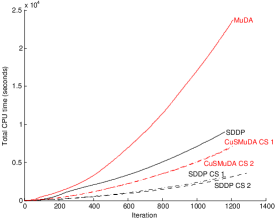
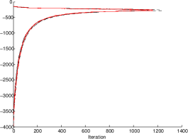
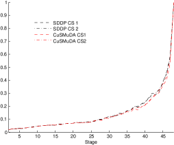
For Instance 1, the mean proportion (over the iterations of the algorithm) of cuts selected by all variants with cut selection, i.e., SDDP CS 1, SDDP CS 2, CuSMuDA CS 1, and CuSMuDA CS 2, tends to increase with the stage and is very low for nearly all stages (at most 0.1 until stage 30 and at most 0.2 until stage 40, knowing that there are $T=48$ stages for that instance); see the bottom plot of Figure 2 which represents the evolution of the mean proportion of cuts selected as a function of the stage. This makes sense since at the last stage, the cuts for functions $\mathfrak{Q}_{T}(\cdot,\xi_{Tj})$ are exact (and as we recalled, all of them are selected with CuSMuDA CS 1) but not necessarily for stages $t<T$ because for these stages approximate recourse functions are used and the approximation errors propagate backward. Therefore it is expected that at the early stages old cuts (computed at the first iterations using crude approximations of the recourse functions) will probably not be selected. Additionally, another reason why fewer cuts are selected in earlier stages may come from the fact that there are fewer distinct sampled points in the state-space.

Moreover the proportion of cuts selected is very similar for all variants.

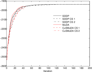
Since the degradation in the upper and lower bound for variants with cut selection is very limited (see the evolution of the upper and lower bounds along iterations for all methods on the top right plot of Figure 2), the number of iterations required to solve Instance 1 by these variants and their counterpart without cut selection is similar.

Figure 2. Top left: total CPU time (in seconds) as a function of the number of iterations for SDDP, SDDP CS 1, SDDP CS 2, MuDA, CuSMuDA CS 1, and CuSMuDA CS 2 to solve Instance 1. Top right: evolution of the upper bounds $z_{\sup}^{i}$ and lower bounds $z_{\inf}^{i}$ along the iterations of SDDP, SDDP CS 1, SDDP CS 2, MuDA, CuSMuDA CS 1, and CuSMuDA CS 2 to solve Instance 1 (no legend is given on this plot since all curves are almost identical). Bottom: mean proportion of cuts (over the iterations of the algorithm) selected for stages $t=2,\ldots,T=48$ by SDDP CS 1, SDDP CS 2, CuSMuDA CS 1, and CuSMuDA CS 2 to solve Instance 1.

Therefore, variants with cut selection are much quicker and the quickest variant with cut selection is the one requiring the least number of iterations; see the top left plot of Figure 2 which plots the total CPU time as a function of the number of iterations.

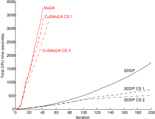
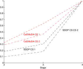
For Instance 2 solved by MuDA and its variants with cut selection, we refer to Figure 3. We see on this figure that these variants again select a very small proportion of cuts for stages 2 and 3 (here, the number of stages is $T=4$) and that this proportion increases with the stage. The degradation in the lower bound for variants with cut selection is larger than with Instance 1 but is still very limited. Therefore, variants with cut selection are much quicker. CuSMuDA CS 2 requires less cuts than CuSMuDA CS 1 but more iterations and CPU time for both variants is similar.

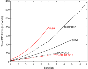
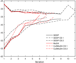
To explain patterns (P2) and (P3), we consider Instance 2 for SDDP, of type (P2), Instance 3 for SDDP and MuDA, of type (P3), and refer to Figures 3 and 4 which are the analogues of Figure 2 for Instances 2 and 3.

Figure 3. Top left: total CPU time (in seconds) as a function of the number of iterations for SDDP, SDDP CS 1, SDDP CS 2, MuDA, CuSMuDA CS 1, and CuSMuDA CS 2 to solve Instance 2. Top right: evolution of the lower bounds $z_{\inf}^{i}$ along the iterations of SDDP, SDDP CS 1, SDDP CS 2, MuDA, CuSMuDA CS 1, and CuSMuDA CS 2 to solve Instance 2. Bottom: mean proportion of cuts (over the iterations of the algorithm) selected for stages $t=2,3,T=4$, by SDDP CS 1, SDDP CS 2, CuSMuDA CS 1, and CuSMuDA CS 2 to solve Instance 2.

Figure 4. Top left: total CPU time (in seconds) as a function of the number of iterations for SDDP, SDDP CS 1, SDDP CS 2, MuDA, and CuSMuDA CS 2 to solve Instance 3 (we did not represent the curve for CuSMuDA CS 1 since the total CPU time with CuSMuDA CS 1 is much larger). Top right: evolution of the upper bounds $z_{\sup}^{i}$ and lower bounds $z_{\inf}^{i}$ along the iterations of SDDP, SDDP CS 1, SDDP CS 2, MuDA, CuSMuDA CS 1, and CuSMuDA CS 2 to solve Instance 3. Bottom: mean proportion of cuts (over the iterations of the algorithm) selected for stages $t=2,\ldots,T=12$, by SDDP CS 1, SDDP CS 2, CuSMuDA CS 1, and CuSMuDA CS 2 to solve Instance 3.

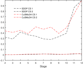On Figure 3, we see that on Instance 2, SDDP CS 1 and SDDP CS 2 select a small proportion of cuts for stages $2$ and $3$ (recall that this is an instance with $T=4$ stages) and require, as SDDP, 200 iterations (the evolution of the lower bound along iterations is similar for all 3 methods). Moreover, SDDP CS 2 selects significantly less cuts than SDDP CS 1 for stages 2 and 3 and therefore is much quicker than SDDP CS 1. This means that a large number of cuts have the same value at some trial points and for each such trial point if SDDP CS 1 selects all these cuts CuSMuDA CS 2 only selects the oldest of these cuts.

Instance 3 is an example of a problem where LML 1 cut selection strategy selects a very small number of cuts for all stages whereas Level 1 selects many more cuts, both for MuDA and SDDP (see Figure 4). On top of that, SDDP CS 1 (resp. CuSMuDA CS 1) needs more iterations than SDDP and SDDP CS 2 (resp. MuDA and CuSMuDA CS 2). Therefore the CPU time needed to solve Instance 3 with SDDP CS 1 (resp. CuSMuDA CS 1) is much larger than the CPU time needed to solve this instance with SDDP and SDDP CS 2 (resp. MuDA and CuSMuDA CS 2). This is an example of an instance where the time spent to select the cuts is not compensated by the (small) reduction in CPU time for solving the problems in the backward and forward passes.

Summarizing our observations,

• Pattern (P3) occurs when a variant with cut selection selects a large proportion of cuts and requires too many iterations;

• Patterns (P1) and (P2) occur when variants with cut selection select a small number of cuts and do not need much more iterations than the variant without cut selection. In this situation, (P1) occurs either when (i) both variants with cut selection select a similar number of cuts or when (ii) one variant selects less cuts than the other but needs slightly more iterations.

One last comment is now in order. We have already observed that on all experiments, Level 1 and Territory Algorithm cut selection strategies, i.e., SDDP CS 1 and CuSMuDA CS 1, correctly select all cuts at the final stage. However, a crude implementation of the Level 1 pseudo-code given in Figure 1 resulted in the elimination of cuts at the final stage. This comes from the fact that approximate solutions of the optimization subproblems are computed. Therefore two optimization problems could compute the same cuts but the solver may return two different (very close) approximate solutions. Similarly, a cut may be in theory the highest at some point (for instance cut $\mathcal{C}_{Tj}^{k}$ is, in theory, the highest at $x_{T-1}^{k}$) but numerically the value of another cut at this point may be deemed slightly higher, because of numerical errors. The remedy is to introduce a small error term $\varepsilon_{0}$ ($\varepsilon_{0}=10^{-6}$ in our experiments) such that the values $V_{1}$ and $V_{2}$ of two cuts $\mathcal{C}_{1}$ and $\mathcal{C}_{2}$ at a trial point are considered equal if $|V_{2}-V_{1}|\leq\varepsilon_{0}\max(1,|V_{1}|)$ while $\mathcal{C}_{1}$ is above $\mathcal{C}_{2}$ at this trial point if $V_{1}\geq V_{2}+\varepsilon_{0}\max(1,|V_{1}|)$. Therefore the pseudo-codes of Level 1 and LML 1 given in Figure 1 need to be modified. The corresponding pseudo-codes taking into account the approximation errors are given in Figure 6 in the Appendix. Adding cuts that improve the approximation by more than some threshold $\varepsilon_{0}$ was also used in [23].

5.2. Inventory management

5.2.1. Model

We consider the $T$-stage inventory management problem given in (Shapiro et al. 2009). For each stage $t=1,\ldots,T$, on the basis of the inventory level $x_{t-1}$ at the beginning of period $t$, we have to decide on the quantity $y_{t}-x_{t-1}$ of a product to buy so that the inventory level becomes $y_{t}$. Given demand $\xi_{t}$ for that product for stage $t$, the inventory level is $x_{t}=y_{t}-\xi_{t}$ at the beginning of stage $t+1$. The inventory level can become negative, in which case a backorder cost is paid. If one is interested in minimizing the average cost over the optimization period, we need to solve the following dynamic programming equations: for $t=1,\ldots,T$, defining $\mathcal{Q}_{t}(x_{t-1})=\mathbb{E}_{\xi_{t}}[\mathfrak{Q}_{t}(x_{t-1},\xi_{t})]$, the stage $t$ problem is

$$\mathfrak{Q}_{t}(x_{t-1},\xi_{t})=\left\{\begin{array}[]{l}\inf c_{t}(y_{t}-x_{t-1})+b_{t}(\xi_{t}-y_{t})_{+}+h_{t}(y_{t}-\xi_{t})_{+}+\mathcal{Q}_{t+1}(x_{t})\\ x_{t}=y_{t}-\xi_{t},y_{t}\geq x_{t-1},\end{array}\right.$$

where $c_{t}$ is the unit buying cost, $h_{t}$ is the holding cost, and $b_{t}$ the backorder cost. The optimal mean cost is $\mathcal{Q}_{1}(x_{0})$ where $x_{0}$ is the initial stock.

In what follows, we present the results of numerical simulations obtained solving this problem with SDDP, SDDP CS 1, SDDP CS 2, MuDA, CuSMuDA CS 1, and CuSMuDA CS 2 (we used the same notation as before to denote the solution methods).

5.2.2. Numerical results

We consider six values for the number of stages $T$ ($T\in\{5,10,15,20,25,30\}$) and for fixed $T$, the following values of the problem and algorithm parameters are taken:

• $c_{t}=1.5+\cos(\frac{\pi t}{6}),b_{t}=2.8,h_{t}=0.2,M_{t}=M$ for all $t=1,\ldots,T$,

• $x_{0}=10$, $p_{ti}=\frac{1}{M}=\frac{1}{20}$ for all $t,i$,

• $\xi_{1}={\overline{\xi_{1}}}$ and $(\xi_{t1},\xi_{t2},\ldots,\xi_{tM})$ corresponds to a sample from the distribution of ${\overline{\xi_{t}}}(1+0.1\varepsilon_{t})$ for i.i.d $\varepsilon_{t}\sim\mathcal{N}(0,1)$ for $t=2,\ldots,T$, where ${\overline{\xi_{t}}}=5+0.5t$,

• for the stopping criterion, in (24) $\alpha=0.025$ and $N=S=200$, and $\varepsilon=0.05$ in (27).
  

Checking the implementations. As for the portfolio problem, for each value of $T\in\{5,10,15,20,25,30\}$, we checked that upper and lower bounds computed by all 6 methods are very close for the three algorithms at the final iteration.

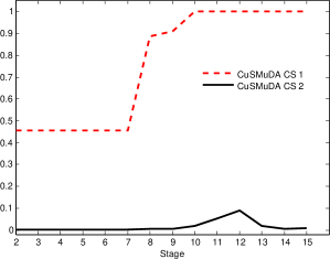
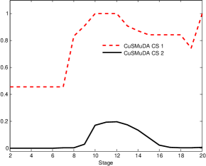
Computational time and proportion of cuts selected. Table 3 shows the CPU time needed to solve our six instances of inventory management problems. For SDDP, all variants with cut selection yield important reduction in CPU time and SDDP CS 2, that uses LML 1, is by far the quickest on 5 instances. For MuDA, Level 1 is not efficient (CPU time with CuSMuDA CS 1 is much larger than CPU time with MuDA) whereas LML 1 allows us to drastically reduce CPU time. As for instances of the portfolio problem of type (P3), the fact that CuSMuDA CS 1 is much slower than both CuSMuDA CS 2 and MuDA is that it requires a similar number of iterations and selects much more cuts than CuSMuDA CS 2 which selects very few cuts for all stages, as can be seen on Figure 5 which represents the mean proportion of cuts selected for CuSMuDA CS 1 and CuSMuDA CS 2 as a function of the number of stages for two instances.

	SDDP	SDDP CS 1	SDDP CS 2	MuDA	CuSMuDA CS 1	CuSMuDA CS 2
$T=5$	0.57	0.48	0.18	1.57	2.90	0.22
$T=10$	5.9	1.22	1.42	26.33	43.07	1.68
$T=15$	21.9	20.4	4.56	106.52	178.08	8.07
$T=20$	28.6	31.2	9.94	158.10	245.24	19.43
$T=25$	36.5	62.8	9.61	189.27	405.58	22.64
$T=30$	77.7	63.6	18.30	363.86	575.53	56.62

Table 3. Computational time (in minutes) for solving instances of the inventory problem of Section 5.2.1 for $M=20$ with SDDP, SDDP CS 1, SDDP CS 2, MuDA, CuSMuDA CS 1, and CuSMuDA CS 2.

$T=15,M=20$	$T=20,M=20$

Figure 5. Mean proportion of cuts (over the iterations of the algorithm) selected for stages $t=2,\ldots,T$ for CuSMuDA CS 1 and CuSMuDA CS 2 for the inventory problem for $M=20$.

6. Conclusion

We proposed CuSMuDA, a combination of a class of cut selection strategies with Multicut Decomposition algorithms to solve multistage stochastic linear programs. We proved the almost sure convergence of the method in a finite number of iterations and obtained as a by-product the almost sure convergence in a finite number of iterations of SDDP combined with this class of cut selection strategies.

Numerical experiments on many instances of a portfolio and of an inventory problem have shown that combining LML 1 cut selection with SDDP (resp. MuDA) allows us in general to reduce considerably the CPU time of SDDP (resp. MuDA). There are, however, situations where a variant with selection is slower than its counterpart without cut selection.

It would be interesting to test CuSMuDA and the Limited Memory variant of Level 1 (both for MuDA and SDDP) on other types of stochastic programs and to extend the analysis to nonlinear stochastic programs.

Appendix

Level 1

Limited Memory Level 1

$I_{tj}^{k}=\{k\}$, $m_{tj}^{k}=\mathcal{C}_{tj}^{k}(x_{t-1}^{k})$. For $\ell=1,\ldots,k-1$, If $\mathcal{C}_{tj}^{k}(x_{t-1}^{\ell})>m_{tj}^{\ell}+\varepsilon_{0}\max(1,|m_{tj}^{\ell}|)$         $I_{tj}^{\ell}=\{k\},\;m_{tj}^{\ell}=\mathcal{C}_{tj}^{k}(x_{t-1}^{\ell})$ Else if $|\mathcal{C}_{tj}^{k}(x_{t-1}^{\ell})-m_{tj}^{\ell}|\leq\varepsilon_{0}\max(1,|m_{tj}^{\ell}|)$         $I_{tj}^{\ell}=I_{tj}^{\ell}\cup\{k\}$ End If If $\mathcal{C}_{tj}^{\ell}(x_{t-1}^{k})>m_{tj}^{k}+\varepsilon_{0}\max(1,|m_{tj}^{k}|)$         $I_{tj}^{k}=\{\ell\},\;m_{tj}^{k}=\mathcal{C}_{tj}^{\ell}(x_{t-1}^{k})$ Else if $|\mathcal{C}_{tj}^{\ell}(x_{t-1}^{k})-m_{tj}^{k}|\leq\varepsilon_{0}\max(1,|m_{tj}^{k}|)$         $I_{tj}^{k}=I_{tj}^{k}\cup\{\ell\}$ End If End For

$I_{tj}^{k}=\{1\}$, $m_{tj}^{k}=\mathcal{C}_{tj}^{1}(x_{t-1}^{k})$. For $\ell=1,\ldots,k-1$, If $\mathcal{C}_{tj}^{k}(x_{t-1}^{\ell})>m_{tj}^{\ell}+\varepsilon_{0}\max(1,|m_{tj}^{\ell}|)$         $I_{tj}^{\ell}=\{k\},\;m_{tj}^{\ell}=\mathcal{C}_{tj}^{k}(x_{t-1}^{\ell})$ End If If $\mathcal{C}_{tj}^{\ell+1}(x_{t-1}^{k})>m_{tj}^{k}+\varepsilon_{0}\max(1,|m_{tj}^{k}|)$         $I_{tj}^{k}=\{\ell+1\},\;m_{tj}^{k}=\mathcal{C}_{tj}^{\ell+1}(x_{t-1}^{k})$ End If End For

Figure 6. Pseudo-codes for selecting the cuts using Level 1 and Limited Memory Level 1 taking into account approximation errors.

References

- [1] E. D. Andersen and K.D. Andersen. The MOSEK optimization toolbox for MATLAB manual. Version 7.0, 2013.
- [2] T. Asamov and W. Powell. Regularized decomposition of high-dimensional multistage stochastic programs with markov uncertainty. Available at: https://arxiv.org/abs/1505.02227, 2015.
- [3] A. Ben-Tal, T. Margalit, and A. Nemirovski. Robust modeling of multi-stage portfolio problems. in: H. Frenk, K. Roos, T. Terlaky, S. Zhang, Eds., High Performance Optimization, Kluwer Academic Publishers, pages 303–328, 2000.
- [4] M. Best and J. Hlouskova. An algorithm for portfolio optimization with variable transaction costs, part 1: Theory. Journal of Optimization Theory and Applications, 135:563–581, 2007.
- [5] J. Birge and F. Louveaux. Introduction to Stochastic Programming. Springer-Verlag, New York, 1997.
- [6] J.R. Birge. Decomposition and partitioning methods for multistage stochastic linear programs. Oper. Res., 33:989–1007, 1985.
- [7] J.R. Birge and C. J. Donohue. The Abridged Nested Decomposition Method for Multistage Stochastic Linear Programs with Relatively Complete Recourse. Algorithmic of Operations Research, 1:20–30, 2001.
- [8] J.R. Birge, C.J. Donohue, D.F. Holmes, and O.G. Svintsitski. A parallel implementation of the nested decomposition algorithm for multistage stochastic linear programs. Mathematical Programming, 75:327–352, 1996.
- [9] J.R. Birge and F.V. Louveaux. A multicut algorithm for two-stage stochastic linear programs. European Journal of Operational Research, 34:384–392, 1988.
- [10] Z.L. Chen and W.B. Powell. Convergent Cutting-Plane and Partial-Sampling Algorithm for Multistage Stochastic Linear Programs with Recourse. J. Optim. Theory Appl., 102:497–524, 1999.
- [11] H. Gassmann. Mslip: A computer code for the multistage stochastic linear programming problem. Math. Program., 47:407–423, 1990.
- [12] S. Gaubert, W. McEneaney, and Z. Qu. Curse of dimensionality reduction in max-plus based approximation methods: Theoretical estimates and improved pruning algorithms. 50th IEEE Conference on Decision and Control and European Control Conference (CDC-ECC), pages 1054–1061, 2011.
- [13] P. Girardeau, V. Leclere, and A.B. Philpott. On the convergence of decomposition methods for multistage stochastic convex programs. Mathematics of Operations Research, 40:130–145, 2015.
- [14] V. Guigues. SDDP for some interstage dependent risk-averse problems and application to hydro-thermal planning. Computational Optimization and Applications, 57:167–203, 2014.
- [15] V. Guigues. Convergence analysis of sampling-based decomposition methods for risk-averse multistage stochastic convex programs. SIAM Journal on Optimization, 26:2468–2494, 2016.
- [16] V. Guigues. Dual dynamic programing with cut selection: Convergence proof and numerical experiments. European Journal of Operational Research, 258:47–57, 2017.
- [17] V. Guigues and W. Römisch. Sampling-based decomposition methods for multistage stochastic programs based on extended polyhedral risk measures. SIAM J. Optim., 22:286–312, 2012.
- [18] V. Guigues and W. Römisch. SDDP for multistage stochastic linear programs based on spectral risk measures. Operations Research Letters, 40:313–318, 2012.
- [19] V. Guigues, W. Tekaya, and M. Lejeune. Regularized decomposition methods for deterministic and stochastic convex optimization and application to portfolio selection with direct transaction and market impact costs. Optimization OnLine, 2017.
- [20] M. Hindsberger and A. B. Philpott. Resa: A method for solving multi-stage stochastic linear programs. SPIX Stochastic Programming Symposium, 2001.
- [21] G. Infanger and D. Morton. Cut sharing for multistage stochastic linear programs with interstage dependency. Math. Program., 75:241–256, 1996.
- [22] V. Kozmik and D.P. Morton. Evaluating policies in risk-averse multi-stage stochastic programming. Mathematical Programming, 152:275–300, 2015.
- [23] N. Löhndorf, D. Wozabal, and S. Minner. Optimizing trading decisions for hydro storage systems using approximate dual dynamic programming. Operations Research, 61:810–823, 2013.
- [24] W.M. McEneaney, A. Deshpande, and S. Gaubert. Curse of complexity attenuation in the curse of dimensionality free method for HJB PDEs. American Control Conference, pages 4684–4690, 2008.
- [25] M.V.F. Pereira and L.M.V.G Pinto. Multi-stage stochastic optimization applied to energy planning. Math. Program., 52:359–375, 1991.
- [26] Laurent Pfeiffer, Romain Apparigliato, and Sophie Auchapt. Two methods of pruning benders’ cuts and their application to the management of a gas portfolio. Research Report RR-8133, hal-00753578, 2012.
- [27] A. Philpott and V. de Matos. Dynamic sampling algorithms for multi-stage stochastic programs with risk aversion. European Journal of Operational Research, 218:470–483, 2012.
- [28] A. Philpott, V. de Matos, and E. Finardi. Improving the performance of stochastic dual dynamic programming. Journal of Computational and Applied Mathematics, 290:196–208, 2015.
- [29] A. B. Philpott and Z. Guan. On the convergence of stochastic dual dynamic programming and related methods. Oper. Res. Lett., 36:450–455, 2008.
- [30] W.P. Powell. Approximate Dynamic Programming. John Wiley and Sons, 2nd edition, 2011.
- [31] A. Ruszczyński. Parallel decomposition of multistage stochastic programming problems. Math. Programming, 58:201–228, 1993.
- [32] A. Shapiro. Analysis of stochastic dual dynamic programming method. European Journal of Operational Research, 209:63–72, 2011.
- [33] A. Shapiro, D. Dentcheva, and A. Ruszczyński. Lectures on Stochastic Programming: Modeling and Theory. SIAM, Philadelphia, 2009.
- [34] A. Shapiro, W. Tekaya, J.P. da Costa, and M.P. Soares. Risk neutral and risk averse stochastic dual dynamic programming method. European Journal of Operational Research, 224:375–391, 2013.
- [35] A. Shapiro, W. Tekaya, J.P. da Costa, and M.P. Soares. Worst-case-expectation approach to optimization under uncertainty. Oper. Res., 61:1435–1449, 2013.
- [36] W. Zhang, H. Rahimian, and G. Bayraksan. Decomposition algorithms for risk-averse multistage stochastic programs with application to water allocation under uncertainty. INFORMS Journal on Computing, 28:385–404, 2016.