Asteroseismic masses, ages, and core properties of $\gamma$ Doradus stars using gravito-inertial dipole modes and spectroscopy

Abstract

The asteroseismic modelling of period spacing patterns from gravito-inertial modes in stars with a convective core is a high-dimensional problem. We utilise the measured period spacing pattern of prograde dipole gravity modes (acquiring $\Pi_{0}$), in combination with the effective temperature ($T_{\rm eff}$) and surface gravity ($\log g$) derived from spectroscopy, to estimate the fundamental stellar parameters and core properties of 37 $\gamma$ Doradus ($\gamma$ Dor) stars whose rotation frequency has been derived from Kepler photometry. We make use of two 6D grids of stellar models, one with step core overshooting and one with exponential core overshooting, to evaluate correlations between the three observables $\Pi_{0}$, $T_{\rm eff}$, and $\log g$ and the mass, age, core overshooting, metallicity, initial hydrogen mass fraction and envelope mixing. We provide multivariate linear model recipes relating the stellar parameters to be estimated to the three observables ($\Pi_{0}$, $T_{\rm eff}$, $\log g$). We estimate the (core) mass, age, core overshooting and metallicity of $\gamma$ Dor stars from an ensemble analysis and achieve relative uncertainties of $\sim\!10$ per cent for the parameters. The asteroseismic age determination allows us to conclude that efficient angular momentum transport occurs already early on during the main sequence. We find that the nine stars with observed Rossby modes occur across almost the entire main-sequence phase, except close to core-hydrogen exhaustion. Future improvements of our work will come from the inclusion of more types of detected modes per star, larger samples, and modelling of individual mode frequencies.

1 Introduction

The photometric data provided by space-based missions such as CoRoT (Auvergne et al., 2009) and Kepler (Koch et al., 2010) have heralded a new era for asteroseismology. Here, we are concerned with gravito-inertial asteroseismology, i.e., the study of gravity modes (g modes) in rotating intermediate-mass stars. Such modes are subject to both the Coriolis force and buoyancy as restoring forces. While CoRoT data led to the first discoveries of period spacings of gravity-mode pulsators in the core-hydrogen burning phase (Degroote et al., 2010; Pápics et al., 2012), it did not allow the identification of the angular degree of these detected oscillations without ambiguity. Secure mode identification had to await nearly uninterrupted time series photometry with at least a factor ten longer time base, such as that assembled with the Kepler space telescope (Borucki et al., 2010). Meanwhile, lots of progress has been made on the observational side in this topic over the past few years with firm detections of period spacing patterns reported in Pápics et al. (2014, 2015); Kurtz et al. (2014); Saio et al. (2015); Van Reeth et al. (2015a); Schmid et al. (2015); Van Reeth et al. (2016); Murphy et al. (2016); Guo et al. (2016); Ouazzani et al. (2017); Saio et al. (2017); Saio et al. (2018); Szewczuk & Daszyńska-Daszkiewicz (2018) and Li et al. (2019).

As shown in these papers, we have now reached the stage where tens of gravity-mode frequencies have been measured in these pulsators with sufficient precision to identify their mode degree from the 4-year nominal Kepler light curves and hence to start testing and improving stellar structure theory of intermediate-mass stars.

Forward modelling applications to a few stars have shown the need of core overshooting and envelope mixing in both B-type and F-type gravity-mode pulsators, in order to be able to explain the measured mode trapping properties (Moravveji et al., 2015, 2016; Schmid & Aerts, 2016). Moreover, the near-core rotation rates derived from the g modes (Van Reeth et al., 2016; Ouazzani et al., 2017; Van Reeth et al., 2018) have revealed shortcomings in stellar evolution theory in terms of angular momentum transport, both during the core-hydrogen burning phase (Rogers, 2015; Aerts et al., 2017; Townsend et al., 2018; Ouazzani et al., 2018) and in the red giant phase (Mosser et al., 2015; Eggenberger et al., 2017; Gehan et al., 2018) – see Aerts et al. (2019) for a recent extensive review.

Since the evolution of a star is greatly affected by the stellar rotation profile (Maeder, 2009), the opportunity to calibrate theoretical stellar models from empirically derived angular momentum distributions in stellar interiors at different evolutionary stages is of major importance. In order to compute these angular momentum distributions, the mass and radius of the star as a whole and of its convective core have to be estimated, as well as the star’s age. Given that forward asteroseismic modelling of intermediate-mass stars is a high dimensional problem (+6D, Aerts et al., 2018), a robust statistical methodology is needed.

In this paper, we explore the feasibility of estimating the most important stellar parameters, i.e., (core) mass, core overshooting, initial hydrogen mass fraction, metallicity, the amount of envelope mixing, and age (or age-proxy) of $\gamma$ Doradus (henceforth $\gamma$ Dor) stars. While these pulsators of spectral type late-A to early-F were already known to have g modes excited by a flux blocking mechanism from ground-based studies (e.g., Kaye et al., 1999; Guzik et al., 2000; Dupret et al., 2005; Cuypers et al., 2009; Bouabid et al., 2013), the derivation of g-mode period spacings had to await the long-term uninterrupted Kepler data (e.g., Bedding et al., 2015; Van Reeth et al., 2015a, b).

Van Reeth et al. (2016); Van Reeth et al. (2018) and Ouazzani et al. (2017) have developed methods to infer the near-core rotation frequency from the slope of the measured period spacing pattern of $\gamma$ Dor stars. These authors applied their methods to ensembles of 40 and 4 stars, respectively, of such gravito-inertial pulsators. Here, we consider the sample by Van Reeth et al. (2016) because 37 of these stars have been monitored with high-resolution spectroscopy (Tkachenko et al., 2013) and the asymptotic period spacing from their prograde sectoral dipole modes, effective temperatures, surface gravities and metallicity have been determined in a homogeneous way.

We explore the modelling capacity of the combined seismic parameter for dipole modes (in the non-rotating limit), $\Pi_{0}$, and the spectroscopically derived effective temperature, $T_{\rm eff}$ and surface gravity, $\log g$, as a major simplification of typical forward modelling that is based on the fitting of all the individual g-mode frequencies. In our approach, we first derive correlations between the the seismic parameter $\Pi_{0}$, the effective temperature and surface gravity on one hand, and the correlation between these three observables and the stellar parameters varied in two 6D stellar model grids on the other hand. Previous studies in the literature have derived correlations between the stellar mass, metallicity, and step overshooting for low-order modes in $\beta$ Cep stars (e.g., Briquet et al., 2007; Walczak et al., 2013) and for high-order g-modes in a Kepler slowly pulsating B-type star (Moravveji et al., 2015). In Section 2, we investigate correlations between mass, central and initial hydrogen fraction, metallicity, the amount of envelope mixing, and the mass and radius of the convective core, by means of linear multivariate regression to investigate the correlations between the parameters in a simple manner. We do this for both a step and an exponential core overshooting formalism since it was recently shown that g modes potentially allow for these two overshooting prescriptions to be distinguished (Pedersen et al., 2018). In particular, we also investigate how well a benchmark model – based on one of these two core overshooting prescriptions – can be approximated by a model based on the other overshooting prescription for the mass range of $\gamma$ Dor stars in Section 3.

Armed with the knowledge of the correlation structure in the two 6D model grids, we explore the capacity of these diagnostics $(\Pi_{0},T_{\rm eff},\log g)$ for parameter estimation from seismic modelling, using the methodology based on maximum likelihood estimation developed in Aerts et al. (2018). The results of our forward modelling are presented in Section 4. In Section 5, we describe our methodology of determining uncertainties from ensemble modelling and we conclude in Section 6.

2 Properties of 6D asteroseismic model grids

2.1 Gravity-mode period spacings

In the framework of the traditional approximation of rotation (TAR; Eckart 1960; Unno et al. 1989), the period of a high-order g-mode can be well approximated by

$$P_{\rm co}\approx\frac{\Pi_{0}}{\sqrt{\lambda_{l,m,s}}}(n_{\rm g}+\alpha_{\rm g}),$$ (1)

with $\lambda$ the eigenvalue of the Laplace tidal equation, depending on the mode geometry (spherical degree $l$ and azimuthal order $m$) and the spin parameter $s=2f_{\rm co}/f_{\rm rot}$ (cf., Townsend, 2003; Bouabid et al., 2013; Van Reeth et al., 2018). The phase term $\alpha_{\rm g}$ depends on the stellar structure and

$$\Pi_{0}\equiv 2\pi^{2}\left(\int_{\rm gc}\frac{N}{r}{\rm d}r\right)^{-1}.$$ (2)

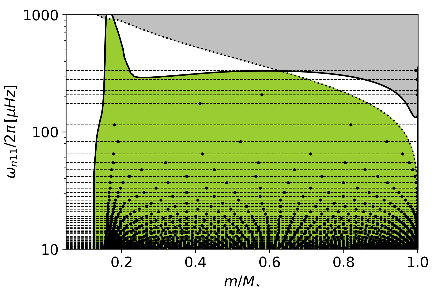
Here, the quantity $N$ is the Brunt-Väisälä frequency and $N/r$ is integrated over the gravity-mode cavity indicated as ‘gc’. An example of such a cavity is shown in Fig. 8 in the Appendix. The asymptotic period spacing of g modes, i.e., the difference in period between two modes of consecutive radial order and same angular degree, in the case of a chemically homogeneous, non-magnetic star is defined in the corotating frame as

$$\Delta P_{\rm co}\approx\frac{\Pi_{0}}{\sqrt{\lambda_{l,m,s}}}.$$ (3)

Depending on the nature of the mode and on the value of the spin parameter, the value of $\lambda_{l,m,s}$ can be approximated by simple analytical expression (cf., Townsend, 2003; Saio et al., 2017, Fig. A1). The spin parameter for the gravito-inertial modes and Rossby modes of the stars in our sample ranges from 1 to 30 (cf., Fig. 2 of Aerts et al., 2017). Given this broad range, it is not obvious to resort to analytical approximations for $\lambda_{l,m,s}$ in the case of $\gamma\,$Dor stars. This motivated Van Reeth et al. (2016) to work with numerical solutions of the Laplace tidal equation.

Comparison between the measured and theoretically predicted gravity-mode periods requires the transformation of the periods to an inertial frame of reference. In the case of a uniform stellar rotation with frequency $f_{\rm rot}$, the periods of the oscillation modes in an inertial frame can be computed as

$$P_{\rm inert}=\frac{1}{f_{\rm co}+mf_{\rm rot}},$$ (4)

where $f_{\rm co}$ is the mode frequency in the corotating frame. We adopt the convention that prograde modes correspond to $m$ > 0.

In the forward modelling applied here, we rely on the observational estimates of $\Pi_{0}$ and of $f_{\rm rot}$ as determined by Van Reeth et al. (2016); Van Reeth et al. (2018). We therefore compute the quantity $\Pi_{0}$ from theoretical stellar evolution models. The diagnostic power of the Brunt-Väisälä frequency and the $\Pi_{0}$ of g modes are well known and have already been exploited asteroseismically since ground-based multi-site white dwarf asteroseismology (Winget et al., 1991; Brassard et al., 1992). The g modes of these compact objects have periods of order a few to ten minutes, such that beating patterns can be covered in observing runs lasting several weeks. Moreover, the rotation period of such stars is of order days, such that the rotational effect on the pulsation modes can be treated from a perturbative approach. The models and g modes in white dwarfs are quite different from those of young stars, hence the parameters that can be deduced from them, as well as the mode trapping properties differ accordingly. From an observational point of view, the application and exploitation of g-mode asteroseismology to core-hydrogen burning stars had to await long-term uninterrupted Kepler photometry, given that the modes have periodicities of order days and beating patterns of years. Moreover, the g modes and rotation rates in these stars have similar periodicities, such that rotation cannot be treated perturbatively, except for a few ultra-slow rotators. This requires dedicated asteroseismic modelling tools suitable to interpret the measured frequencies. Here, we explore and apply aspects of the methodology developed specifically for gravito-inertial modes by Aerts et al. (2018). We first highlight relevant properties of the asteroseismic grids upon which we rely and subsequently exploit the probing power of the three observables ($\Pi_{0}$, $T_{\rm eff}$, $\log g$).

2.2 Correlations among the stellar model parameters

Van Reeth et al. (2016) computed two extensive grids of non-rotating stellar modes with the MESA stellar evolution code (r7385, Paxton et al., 2018, and references therein). These models vary in stellar mass ($M_{\star}$), metallicity ($Z$), diffusive envelope mixing ($D_{\rm mix}$, constant throughout the radiative zone), the extension of the core overshoot region $\alpha_{\rm ov}/f_{\rm ov}$ (i.e., for step/exponential overshoot, expressing the mean free path of a convective fluid element in a radiative region in terms of the local pressure scale height), the initial ($X_{\rm ini}$) and normalised central hydrogen content ($X_{\rm c}^{\prime}=X_{\rm c}/X_{\rm ini}$). The latter is a proxy for the evolutionary stage, hence for the age of the model. In this paper, these two grids of evolution models were extended to lower mass compared to Van Reeth et al. (2016) – a lower limit of 1.2 M_⊙ instead of 1.4 M_⊙. For the models with a convective envelope, we did not consider any undershooting, because this is not important to assess the probing power of high-order g modes.

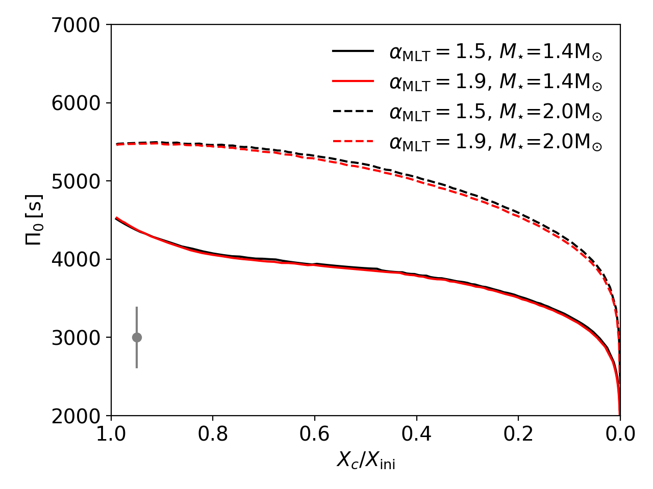
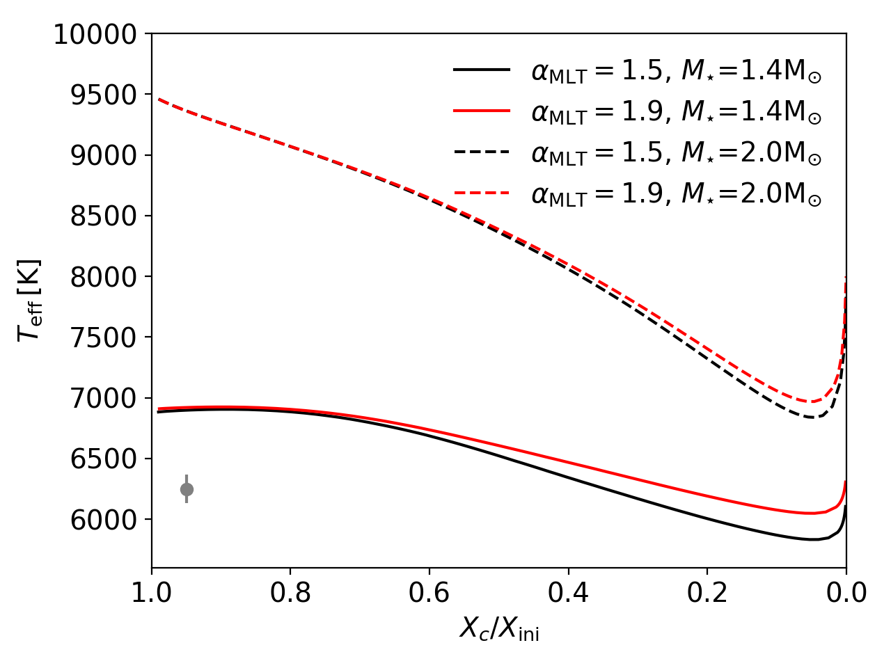
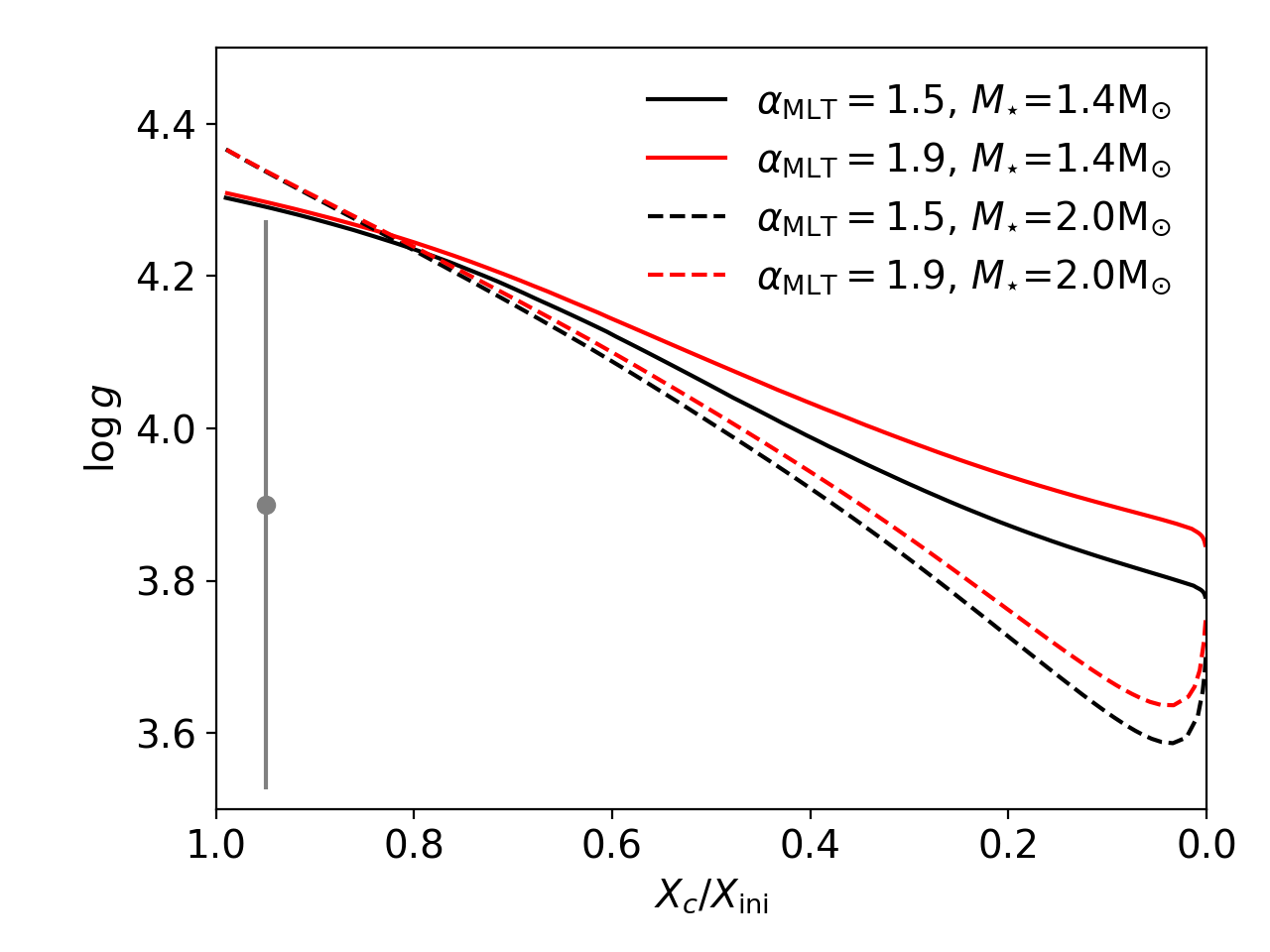
In Table 1, an overview is given of the parameters varied across the two grids and respective step sizes. The efficiency of convection, in our model grids parameterized by the mixing length parameter $\alpha_{\rm MLT}$, was kept fixed at 1.8 throughout the grids. As this was done without further discussion in Van Reeth et al. (2016), we point out here that this parameter does influence the three quantities $\Pi_{0}$, $T_{\rm eff}$, and $\log g$. This is particularly the case for the lower-mass stars in the model grids, since these have the larger convective envelope and are hence affected more by the treatment of convection than the higher-mass stars. Using table 2 from Viani et al. (2018) with the appropriate $\alpha_{\rm MLT}$ value, we made an estimate for the range of the mixing length parameter for the stars in our sample, resulting in $\alpha_{\rm MLT}\in[1.5,1.9]$. Varying $\alpha_{\rm MLT}$ between 1.5 and 1.9, we find that only for the most evolved low-mass stars do the differences in $T_{\rm eff}$ become comparable to typical observational uncertainties, while for $\Pi_{0}$ and $\log g$ the differences are always negligible. We illustrate this in Figs 13–15 in Appendix C for a low-mass and high-mass $\gamma$ Dor model. We do stress that $\alpha_{\rm MLT}$ has a major influence in forward modelling based on fitting individual g-mode frequencies (Aerts et al., 2018, table 2), but that this dependency plays an inferior role compared to the other parameters varied in our grids for forward modelling based on $\Pi_{0}$.

For the modelling done here, we also transformed to the parameter $X_{\rm c}^{\prime}=X_{\rm c}/X_{\rm ini}\in[0,1]$, i.e., to the fraction of the main-sequence duration, as a proxy for the age, rather than using $X_{\rm c}$ itself as in Van Reeth et al. (2016). In this way, the span of $X_{\rm c}^{\prime}$ in the grids is the same for all model tracks ranging from the zero-age main sequence (ZAMS; $X_{\rm c}^{\prime}=1$) to the terminal-age main sequence (TAMS; $X_{\rm c}^{\prime}=0$). After the onset of core-hydrogen burning at the ZAMS, a model requires a few iterations to return to hydrostatic equilibrium and therefore we do not consider any models with $X_{\rm c}^{\prime}>0.99$. In total, the step overshoot grid contains $1530$ evolutionary tracks with $819\,774$ stellar models and the exponential overshoot grid contains $2295$ evolutionary tracks with $1\,300\,590$ stellar models.

For each stellar model in the grids, $\Pi_{0}$ was computed, along with the effective temperature $T_{\rm eff}$ and surface gravity $\log g$, as well as the mass $M_{\rm cc}$ and radius $R_{\rm cc}$ of the convective core. We refer to Table 6 in Appendix D, where we assembled the measured values of $\Pi_{0}$ from Kepler data as determined by Van Reeth et al. (2018) under the assumption of rigid rotation. For the stars with both gravito-inertial prograde dipole modes and Rossby modes, these are improved values compared to those in Van Reeth et al. (2016). The observational estimate of $\Pi_{0}$ for all these stars was deduced along with estimation of the near-core rotation frequency $f_{\rm rot}$ from the slope of the measured period spacing patterns. The relative observational errors for $\Pi_{0}$ range from 0.2 to 26 per cent for the various sample stars. Below, we compare these observables with the theoretical predictions for $\Pi_{0}$ computed for each of the grid models. We recall explicitly that Van Reeth et al. (2016) carefully omitted modes that are trapped to estimate $\Pi_{0}$ and $f_{\rm rot}$ from the data (cf., their figs 4 and 9). These two observed quantities, along with the mode identification, were derived using the TAR to compute $\lambda_{l,m,s}$ with the pulsation code GYRE (Townsend & Teitler, 2013; Townsend et al., 2018) for each of the models in the two extensive 6D grids, which cover the relevant parameter ranges of $\gamma\,$Dor stars. In this way, our observational estimation of $\Pi_{0}$ and $f_{\rm rot}$ does not depend on particular choices of these model parameters.

Parameter	Lower boundary	Upper boundary	Step size
Step overshoot
$M_{\star}$	1.20 M⊙	2.00 M⊙	0.05 M⊙
$Z$	0.010	0.018	0.004
$\log D_{\rm mix}[$cm2s${}^{-1}]$	-1	0	1
$\alpha_{\rm ov}$	0.01	0.300	0.075
$X_{\rm ini}$	0.69	0.73	0.02
$X_{\rm c}^{\prime}$	0	0.99	<0.007
Exponential overshoot
$M_{\star}$	1.20 M⊙	2.00 M⊙	0.05 M⊙
$Z$	0.010	0.018	0.004
$\log D_{\rm mix}[$cm2s${}^{-1}]$	-1	1	1
$f_{\rm ov}$	0.001	0.0300	0.0075
$X_{\rm ini}$	0.69	0.73	0.02
$X_{\rm c}^{\prime}$	0	0.99	<0.007

Table 1: Range of the model grids for which $\Pi_{0}$, $T_{\rm eff}$, and $\log g$ have been computed.

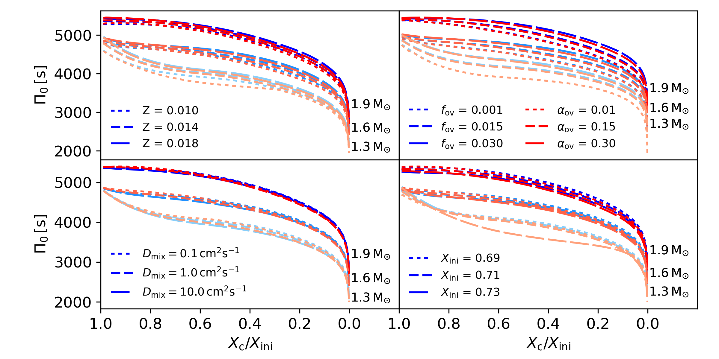
We recall that mixing in the radiative zone had to be introduced in addition to core overshooting in models of B-type pulsators to fit the frequencies of trapped g modes (Moravveji et al., 2015, 2016). In Fig. 1, the evolution of $\Pi_{0}$ as a function of the stellar age is illustrated, where either $X_{\rm ini}$, $Z$, $\alpha_{\rm ov}/f_{\rm ov}$ or $D_{\rm mix}$ is being varied, while the three remaining parameters are kept fixed, for masses 1.3, 1.6, and 1.9 M_⊙. This gives a good visual representation of the dependencies of $\Pi_{0}$ on these four model parameters in the grids. It can be seen that there is no unique monotonic relation between mass, age and $\Pi_{0}$ because the core overshooting, metallicity and initial hydrogen (in this descending order of importance) do have an effect larger than the typical measurement uncertainty of $\Pi_{0}$ deduced from the Kepler light curves (cf., Aerts et al., 2018, for a thorough discussion of theoretical uncertainties on g-mode frequencies). The envelope mixing does not influence the period spacing values as much as the other three parameters. This is entirely as expected, given that the g modes mainly probe the core overshooting, while they are hardly affected by the envelope mixing. However, the mixing at the interface between the overshoot zone and the bottom of the radiative envelope is responsible for the details of the mode trapping and has to be considered when performing frequency fitting as opposed to matching of the asymptotic period spacing (cf., Moravveji et al., 2016; Van Reeth et al., 2016; Pedersen et al., 2018).

Figure 1: Evolution of $\Pi_{0}$ along the main sequence for changing metallicity (top left), amount of core overshooting (top right), the amount of mixing in the radiative zone (bottom left) and initial hydrogen mass fraction (bottom right), for a 1.3-, 1.6- and 1.9-${\rm M}_{\odot}$ star (lightest colour to darkest). The blue lines correspond to an exponential overshooting prescription and the red lines to a step overshooting prescription, both of which consider the radiative temperature gradient in the overshoot zone. When a parameter is not being varied, it is set at $Z=0.014$, $\alpha_{\rm ov}=0.225$, $f_{\rm ov}=0.0225$, $D_{\rm mix}=$1.0\text{\,}{\mathrm{cm}}^{2}\text{\,}{\mathrm{s}}^{-1}$$ and $X_{\rm ini}=0.71$.

2.3 Linear statistical model for $\Pi_{0}$

Following problem set 3 in Aerts et al. (2018), we construct a statistical model for $\Pi_{0}$ based on the stellar input parameters of the model grids by performing a linear multivariate regression, adopting the following form

$$\Pi_{0}=\beta_{0}+\beta_{1}\alpha_{\rm ov}+\beta_{2}D_{\rm mix}+\beta_{3}M_{\star}+\beta_{4}Z+\beta_{5}X_{\rm ini}+\beta_{6}X_{\rm c}^{\prime}+\epsilon,$$ (5)

where $\epsilon$ is the residual and the coefficients $\beta_{i}$ are computed according to an ordinary least-squares regression,

$$\bm{\beta}=(\bm{X}^{\top}\bm{X})^{-1}\bm{X}^{\top}\bm{Y}.$$ (6)

Here, $\bm{Y}$ is a vector with length equal to the number of grid points $i=1,\ldots,q$, containing all values of $\Pi_{0,i}$ and

$$\bm{X}=\begin{pmatrix}1&\alpha_{{\rm ov},1}&D_{{\rm mix},1}&M_{\star,1}&Z_{1}&X_{{\rm ini},1}&X_{\rm c,1}^{\prime}\\ 1&\alpha_{{\rm ov},2}&D_{{\rm mix},2}&M_{\star,2}&Z_{2}&X_{{\rm ini},2}&X_{\rm c,2}^{\prime}\\ \vdots&\vdots&\vdots&\vdots&\vdots&\vdots&\vdots\\ 1&\alpha_{{\rm ov},q}&D_{{\rm mix},q}&M_{\star,q}&Z_{q}&X_{{\rm ini},q}&X_{{\rm c},q}^{\prime}\\ \end{pmatrix}.$$ (7)

For the step overshoot grid, $q=$819\,774$$, while for the exponential overshoot grid, $q=$1\,300\,590$$.

The residual term $\epsilon$ captures the non-linearity in $\Pi_{0}$ as it occurs in the model grids. We point out that both the coefficients $\beta_{i}$ and $\epsilon$ depend on the choices of microphysics that went into the computation of the stellar models. This concerns opacity tables, the equation of state, nuclear reactions and chemical mixtures. The effect of these choices on g-mode pulsation frequencies cannot be represented by a few simple model parameters, as discussed in detail in sections 2 to 4 in Aerts et al. (2018). That paper’s table 2 also includes a detailed quantification and hierarchical ordering of the effect of the choices of micro- and macro-physics when performing forward asteroseismic modelling of main-sequence stars.

	Step overshoot	Exponential overshoot
$\beta_{0}\,({\rm Offset})$	1095.74$\,\pm\,$12.64	1112.30$\,\pm\,$10.05
$\beta_{1}\,(\alpha_{\rm ov})$	-258.2$\,\pm\,$3.6	-3076.99$\,\pm\,$30.43
$\beta_{2}\,(D_{\rm mix})$	-53.0$\,\pm\,$0.6	-7.70$\,\pm\,$0.05
$\beta_{3}\,(M_{\star})$	520.2$\,\pm\,$2.0	631.0$\,\pm\,$1.5
$\beta_{4}\,(Z)$	32236.60$\,\pm\,$87.77	32201.55$\,\pm\,$70.09
$\beta_{5}\,(X_{\rm ini})$	456.17$\,\pm\,$17.74	236.57$\,\pm\,$14.07
$\beta_{6}\,(X_{\rm c}^{\prime})$	2620.4$\,\pm\,$3.4	2716.8$\,\pm\,$2.7
$\beta_{7}\,(M_{\rm cc})$	22176.29$\,\pm\,$33.18	21397.18$\,\pm\,$25.16
$\beta_{8}\,(R_{\rm cc})$	-24236.95$\,\pm\,$65.79	-25246.43$\,\pm\,$50.06

Table 2: Regression coefficients from an ordinary least squares fit for the best statistical model in Eq. (8) according to the BIC for $\Pi_{0}$ (s).

	Step overshoot	Exponential overshoot
$\beta_{0}\,({\rm Offset})$	7995.63$\,\pm\,$11.70	7872.1$\,\pm\,$9.1
$\beta_{1}\,(\alpha_{\rm ov})$	-393.9$\,\pm\,$3.3	-6509.54$\,\pm\,$27.48
$\beta_{2}\,(D_{\rm mix})$	-	-0.48$\,\pm\,$0.04
$\beta_{3}\,(M_{\star})$	2508.7$\,\pm\,$1.9	2351.6$\,\pm\,$1.4
$\beta_{4}\,(Z)$	-87369.35$\,\pm\,$81.21	-84919.61$\,\pm\,$63.29
$\beta_{5}\,(X_{\rm ini})$	-6879.91$\,\pm\,$16.41	-6606.00$\,\pm\,$12.71
$\beta_{6}\,(X_{\rm c}^{\prime})$	-792.5$\,\pm\,$3.1	-720.1$\,\pm\,$2.5
$\beta_{7}\,(M_{\rm cc})$	-11630.93$\,\pm\,$30.69	-7662.64$\,\pm\,$22.72
$\beta_{8}\,(R_{\rm cc})$	39468.86$\,\pm\,$60.87	36305.27$\,\pm\,$45.21

Table 3: Same as Table 2, but for a linear regression in the form of Eq. (8) for $T_{\rm eff}$ (K).

	Step overshoot	Exponential overshoot
$\beta_{0}\,({\rm Offset})$	3.746$\,\pm\,$0.002	3.704$\,\pm\,$0.002
$\beta_{1}\,(\alpha_{\rm ov})$	-0.2478$\,\pm\,$0.0007	-3.577$\,\pm\,$0.006
$\beta_{2}\,(D_{\rm mix})$	-0.0015$\,\pm\,$0.0001	-0.000560$\,\pm\,$0.000009
$\beta_{3}\,(M_{\star})$	-0.2440$\,\pm\,$0.0004	-0.2703$\,\pm\,$0.0003
$\beta_{4}\,(Z)$	-1.22$\,\pm\,$0.02	-0.61$\,\pm\,$0.01
$\beta_{5}\,(X_{\rm ini})$	0.506$\,\pm\,$0.003	0.543$\,\pm\,$0.003
$\beta_{6}\,(X_{\rm c}^{\prime})$	-0.0080$\,\pm\,$0.0006	0.0096$\,\pm\,$0.0005
$\beta_{7}\,(M_{\rm cc})$	-3.592$\,\pm\,$0.006	-2.825$\,\pm\,$0.005
$\beta_{8}\,(R_{\rm cc})$	10.48$\,\pm\,$0.01	10.131$\,\pm\,$0.009

Table 4: Same as Table  2, but for a linear regression in the form of Eq. (8) for $\log g$ ($g$ given in cm^-1s^-2).

Once a value for each of the six input parameters is chosen, the mass and radius of the convective core (denoted as $M_{\rm cc}$ and $R_{\rm cc}$, respectively) then follow. The computation of $M_{\rm cc}$ and $R_{\rm cc}$ in our setup comes through the estimation of the core boundary mixing properties, of which the parameters $f_{\rm ov}$ and $D_{\rm mix}$ are simple representations. With Eq. 5, we represent the $\Pi_{0}$ from the grid models by a multivariate linear statistical estimation, with the aim to have a fast tool to compute model properties for parameter sets that fall within the range of those of the grids but do not coincide with an actual grid point. The fit in Eq. 5 also highlights the correlations among the six parameters that should be kept in mind when trying to fit observed values of $\Pi_{0}$. Since the fit for $\Pi_{0}$ from Eq. 5 is an approximation, there is no longer a unique correspondence between the six input parameters and the values for $M_{\rm cc}$ and $R_{\rm cc}$ for parameter combinations that do not coincide with a grid model. For this reason, we also pay specific attention to $M_{\rm cc}$ and $R_{\rm cc}$.

Figure 2: Evolution from near-ZAMS to TAMS of the mass (top panel) and radius (middle panel) fraction of the convective core for different stellar masses. The evolution of the absolute radius of the convective core is given in the bottom panel. The tracks are for $X_{\rm ini}=0.71$, $Z=0.014$, $D_{\rm mix}=$0.1\text{\,}{\mathrm{cm}}^{2}\text{\,}{\mathrm{s}}^{-1}$$ and $f_{\rm ov}=0.03$.

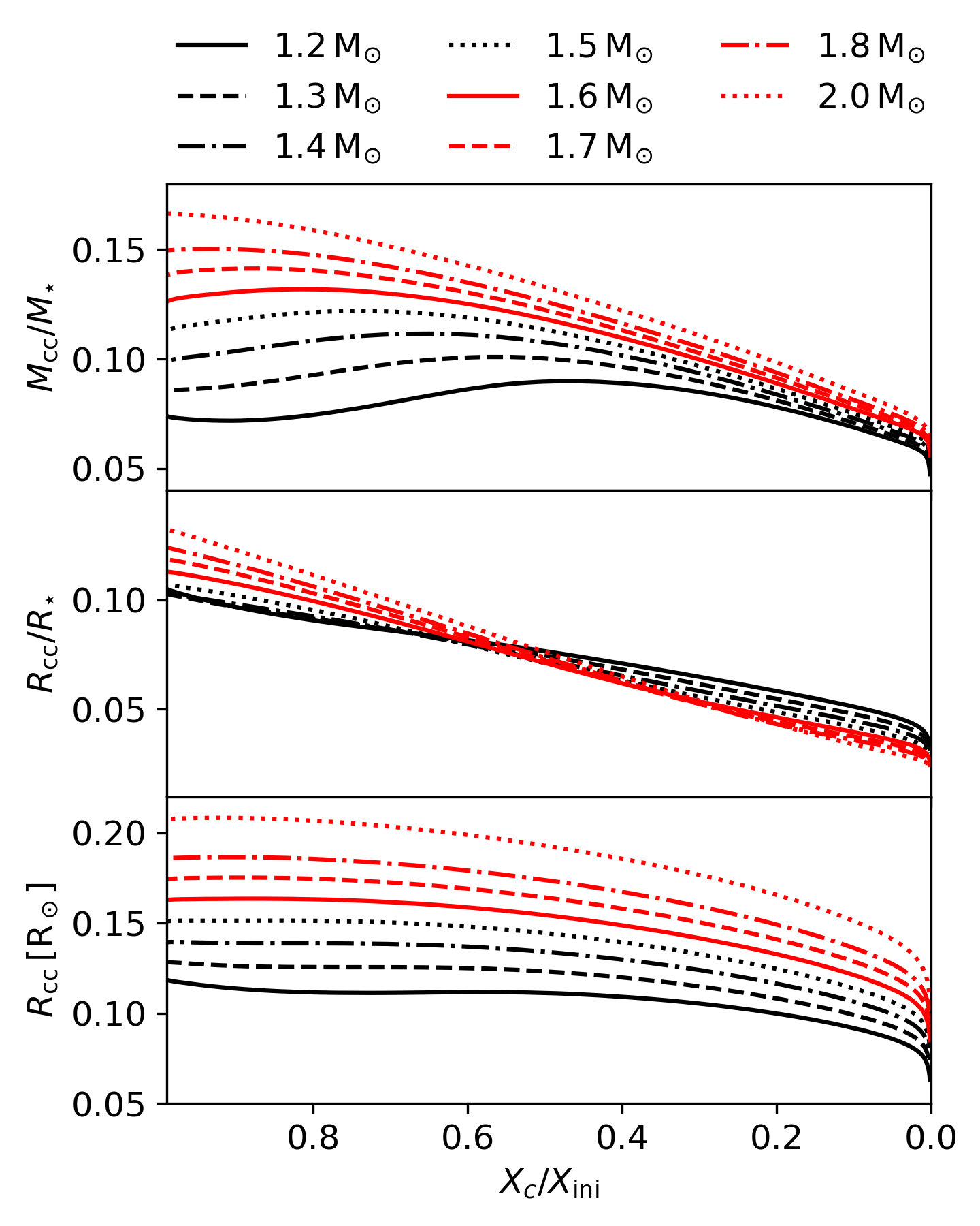
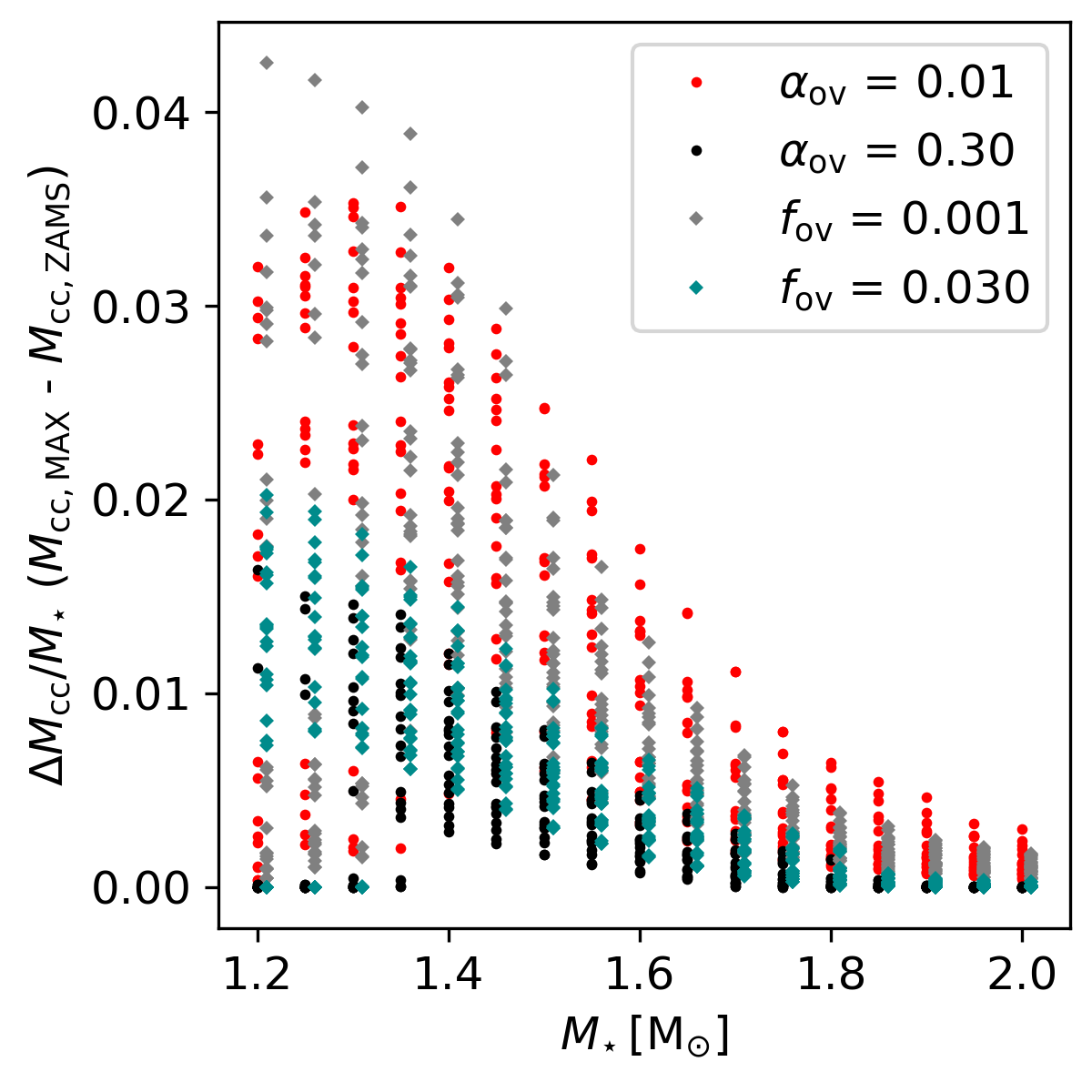
Some of the models in the grids have a growing convective core as the hydrogen-burning progresses, while others have a shrinking convective core, where the transition occurs roughly around a birth mass of 1.6 M_⊙ (cf., Fig. 3.6 in Aerts et al., 2010). This is illustrated for our grids of models in Fig. 2 in terms of the mass and size of the convective core. The phenomenon of a shrinking or growing core lies at the basis of the different correlation structure seen in the different morphologies of the trends for different masses in Fig. 1 in terms of the stellar mass, because the mode cavities are influenced by it during the evolution of the star. Moreover, the extent of the overshoot zone affects the mode trapping and shrinkage or growth of the convective core is influenced by the core overshooting. A summary representation of the maximal growth of the convective core mass during the hydrogen burning, for the entire mass range of the grids and for the two descriptions of the overshooting, is shown in Fig. 3. The gain in core mass gradually decreases as the birth mass increases. It disappears for the most massive stellar models in our grid, as their convective core never grows, but only shrinks after birth. Moreover, the evolution of the core mass is strongly dependent on the value of the overshoot parameter.

The results in Figs 2 and 3 imply that the mass and size of the convective core correlate with $\Pi_{0}$ and that the correlation structure is different for step and exponential overshoot. In order to investigate these dependencies, we add these two quantities to the linear regression model,

$$\begin{split}\Pi_{0}=&\beta_{0}+\beta_{1}\alpha_{\rm ov}+\beta_{2}D_{\rm mix}+\beta_{3}M_{\star}+\beta_{4}Z+\beta_{5}X_{\rm ini}+\beta_{6}X_{\rm c}^{\prime}\\ &+\beta_{7}M_{\rm cc}^{\prime}+\beta_{8}R_{\rm cc}^{\prime}+\epsilon,\end{split}$$ (8)

where $M_{\rm cc}^{\prime}$ is expressed in terms of $M_{\star}$ and $R_{\rm cc}^{\prime}$ is expressed in terms of $R_{\star}$. The core boundary is defined by the Ledoux criterion and we defined the core radius $R_{\rm cc}$ as the point where the Brunt-Väisälä frequency becomes larger than a small threshold $N^{2}>10^{-9}$rad²s^-2. With this set up, we test how a multivariate linear model captures the influence of the core mass and size on $\Pi_{0}$. The results are listed in Table 2 for both grids.

We evaluate the capacity of the multivariate linear model in Eq. (8) by inspecting the square-root of the residual sum of squares of the fit, averaged over all grid points, denoted here as $\sqrt{\langle\rm RSS\rangle}$. We find a value of $252\text{\,}\mathrm{s}$ for step overshoot and $253\text{\,}\mathrm{s}$ for exponential overshoot. As these $\sqrt{\langle\rm RSS\rangle}$ values are comparable with typical measurement uncertainties for $\Pi_{0}$ (Table 6), we conclude that $\Pi_{0}$ can generally be well approximated by a multivariate linear statistical model up to the level of the measurement uncertainties. We do keep in mind that the approximation works less well near the TAMS, where non-linearity of $\Pi_{0}$ is larger than for the other evolutionary phases (cf., Fig. 1). Non-linear multivariate regression to approximate $\Pi_{0}$ (and $T_{\rm eff}$ and $\log g$ further on) is beyond the scope of this paper, but may be interesting to consider as an improvement of our current work for future stellar modelling of near-TAMS pulsators.

Both overshooting prescriptions suggest that the amount of mixing in the radiative zone, $D_{\rm mix}$, has only a modest effect on $\Pi_{0}$, as already reflected in Fig. 1 (see also table 2 in Johnston et al. 2019). However, we expect $D_{\rm mix}$ to have some effect on $\Pi_{0}$ (Van Reeth et al., 2015b) and mainly on the mode trapping, as was shown from forward modelling of g modes in the Kepler B-type pulsator KIC 10526294 (Moravveji et al., 2015). For this reason, we applied the principle of ‘backward selection’, where one eliminates one-by-one the least significant $\beta$-parameter and test if the simpler statistical model is more appropriate (cf., Aerts et al., 2014, where this is explained in more detail and was applied to a similar problem).

A formal way to deduce which statistical model is the more appropriate one is the Bayesian Information Criterion (BIC). Among many other statistical tests, the BIC corrects for the complexity of a statistical model by applying a penalty involving the degrees of freedom (Claeskens & Hjort, 2008) rather than just using the RSS for the model selection. Here, we make an application, using

$${\rm BIC}\equiv q\ln\left(\frac{\rm RSS}{q}\right)+k\ln(q),$$ (9)

where $k$ is the number of free parameters and $q$ is the number of grid points. Starting with a statistical model described by Eq. (8), we compute the corresponding $\beta$ values and their $p$-value, which is defined in the case $q\gg k$ as,

$$p=2[1-\Phi(|t|)],$$ (10)

where $\Phi(|t|)$ is the cumulative standard normal distribution, i.e., the integral of the standard normal density between $-\infty$ and $|t|$. Its argument $t$ is inverse of the relative uncertainty on $\beta$, where the absolute uncertainties are computed by taking the square-root of the diagonal elements of the variance-covariance matrix

$$\bm{V}(\bm{\beta})=(\bm{X}^{\top}\bm{X})^{-1}\sigma^{2},$$ (11)

in which

$$\sigma^{2}=\frac{1}{q-(k+1)}(\bm{Y}-\bm{X\beta})^{\top}(\bm{Y}-\bm{X\beta}),$$ (12)

where for our grids $q\gg k$. Next, we compute a new statistical model where the $\beta_{i}$ with the highest $p$-value from the previous model is omitted, and the new BIC is evaluated. This process is repeated until the BIC of the new model is higher than the previous one. This previous model is then selected to be the optimal statistical model. We refer the interested reader to Aerts et al. (2018) for more details on the statistical framework discussed here. For the statistical models for $\Pi_{0}$, none of the parameters can be omitted according to the BIC criterion.

Figure 3: The maximum difference in mass fraction of the convective core as a function of stellar mass for different overshooting prescriptions. For visibility purposes, the data points corresponding to exponential overshoot have been shifted by 0.01 M_⊙ along the abscissa axis.

2.4 Linear statistical model for $T_{\rm eff}$ and $\log g$

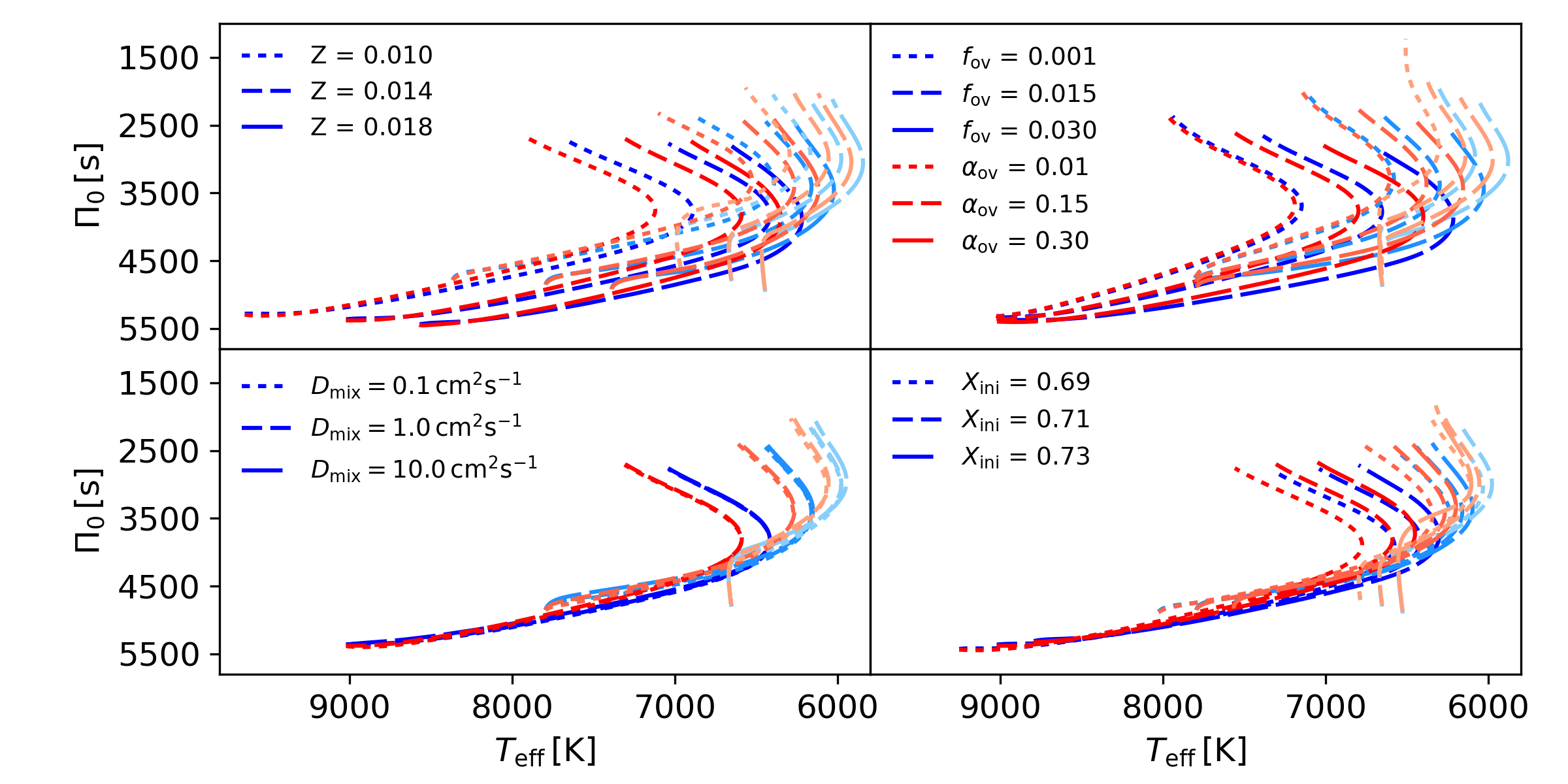
For 37 of the $\gamma$ Dor stars with identified dipole modes in the sample from Van Reeth et al. (2016), a measurement of $T_{\rm eff}$, $\log\,g$, and [M/H] has been obtained from high-resolution spectroscopy. Uncertainties for [M/H] are large ($\sim$100 per cent) (fig. 2 and table 5 in Van Reeth et al., 2015a), but the spectroscopic $T_{\rm eff}$ and $\log\,g$ measurements have relative average precisions of $\sim$2 per cent and $\sim$9 per cent, respectively, for the stars in our sample. As the relative uncertainties of $T_{\rm eff}$ and $\log g$ are comparable with the average precision on $\Pi_{0}$ (for the stars that have spectroscopic data) these observables are good candidates to lift part of the degeneracy between $\Pi_{0}$ and the stellar parameters. For the statistical models of $T_{\rm eff}$, the values of $\sqrt{\langle\rm RSS\rangle}$ are 233 and $229\text{\,}\mathrm{K}$ for step and exponential overshoot, respectively. For $\log g$, the statistical model has $\sqrt{\langle\rm RSS\rangle}=0.05$ dex for both overshooting prescriptions. For $T_{\rm eff}$ this is larger than the typical uncertainty on the observed value measured by Van Reeth et al. (2015a), while for $\log g$ it is significantly better than the observed uncertainties. As shown in Fig. 4, there is a correlation between $\Pi_{0}$ and $T_{\rm eff}$ from near-ZAMS ($X_{\rm c}^{\prime}\sim 0.99$) to near-TAMS ($X_{\rm c}^{\prime}\sim 0$). Again, we vary either $X_{\rm ini}$, $Z$, $\alpha_{\rm ov}/f_{\rm ov}$ or $D_{\rm mix}$ while keeping the other parameters fixed and do this for 1.3, 1.6 and 1.9 M_⊙.

Figure 4: Correlation between the effective temperature $T_{\rm eff}$ and the seismic parameter $\Pi_{0}$ along the main sequence (starting at $X_{\rm c}^{\prime}=0.99$) for changing metallicity (top left), amount of core overshooting (top right), the amount of mixing in the radiative zone (bottom left) and initial hydrogen mass fraction (bottom right), for a 1.3- (lightest colours), 1.6- and 1.9- M_⊙ (darkest colours) star. The blue lines correspond to an exponential overshooting prescription and the red lines to step overshooting prescription, both of which consider the radiative temperature gradient in the overshoot zone. When a parameter is not being varied, it is set at the values $X_{\rm ini}=0.71$, $Z=0.014$, $D_{\rm mix}=$1.0\text{\,}{\mathrm{cm}}^{2}\text{\,}{\mathrm{s}}^{-1}$$, $\alpha_{\rm ov}=0.225$ and $f_{\rm ov}=0.0225$. Both axis have been inverted as to emulate an HR diagram, where the main-sequence stars evolve upwards. The rapid change in $\Pi_{0}$ at constant $T_{\rm eff}$ seen in the tracks of the 1.3 M_⊙ models results from the transition from pre-MS to the MS. These models are already on the main-sequence track and are burning hydrogen in their convective cores.

Analogous to the procedure developed for $\Pi_{0}$ above, we searched for an optimal linear multivariate regression model for $T_{\rm eff}$ and $\log g$. Again, we start with a statistical model as described in Eq. (8) and perform backward selection to see if any redundant parameters can be eliminated, by minimizing the BIC. For exponential overshoot we find that $D_{\rm mix}$ has little effect on $T_{\rm eff}$, but BIC increases when this parameter is not taken into account, suggesting it is not a redundant parameter. In the case of step overshoot, a decrease in BIC of suggests the model without $D_{\rm mix}$ is statistically favoured. The results of these linear regressions for $T_{\rm eff}$ are listed in Table 3. For the statistical models of $\log g$, we find that none of the parameters may be omitted according to the BIC (Table 4).

3 Comparing the two overshooting prescriptions

A major uncertainty in evolution theory of star born with a convective core is the efficiency of the mixing inside the core overshoot region. This translates into the question of the functional prescription of the overshooting. It was recently shown that g modes have the potential to unravel the most appropriate shape, or at least to discriminate between an exponential and a step overshooting prescription (Pedersen et al., 2018).

Here, we compare theoretical models with step versus exponential overshooting prescriptions for the mass range of the $\gamma$ Dor stars to test if we can make a distinction between our two grids of models. We do this by applying the method of parameter estimation and model selection described in Aerts et al. (2018, problem 2). For both overshooting prescriptions, we chose a benchmark model from one grid and fit the corresponding $\Pi_{0}$, effective temperature and surface gravity to the models in the other grid. Adopting the notations in Aerts et al. (2018), we use the subscript to indicate the ‘observational’ values (BM) and a superscript to distinguish between a step (s) and an exponential (e) overshooting prescription. We then compute the optimal (independent) parameters

$$\bm{\theta}_{0}=(M_{\star},X_{\rm c}^{\prime},\alpha_{\rm ov}/f_{\rm ov},Z,X_{\rm ini},D_{\rm mix}),$$ (13)

for both benchmark models according to

$$\bm{\theta}_{0}^{(\rm e)}=\arg\min_{i=1}^{r_{\rm e}^{\prime}}\left[\left(\bm{Y}^{\rm(e)}_{i}-\bm{Y}^{\rm(s)}_{\rm BM}\right)^{\top}\left(\bm{\hat{V}}^{\rm(e)}\right)^{-1}\left(\bm{Y}^{\rm(e)}_{i}-\bm{Y}^{\rm(s)}_{\rm BM}\right)\right],$$ (14)

$$\bm{\theta}_{0}^{(\rm s)}=\arg\min_{j=1}^{r_{\rm s}^{\prime}}\left[\left(\bm{Y}^{\rm(s)}_{j}-\bm{Y}^{\rm(e)}_{\rm BM}\right)^{\top}\left(\bm{\hat{V}}^{\rm(s)}\right)^{-1}\left(\bm{Y}^{\rm(s)}_{j}-\bm{Y}^{\rm(e)}_{\rm BM}\right)\right],$$ (15)

where the index $i=1,\ldots,$819\,774$$ runs over all stellar models in the grid with the exponential overshooting prescription and the index $j=1,\ldots,$1\,300\,590$$ runs over all models in the grid with the step overshooting prescription (superscript on $\bm{\theta_{0}}$ indicates the corresponding grid) and

$$\bm{Y}_{i/j}=\begin{pmatrix}\Pi_{0,i/j}\\ T_{{\rm eff},i/j}\\ \log g_{i/j}\\ \end{pmatrix}.$$ (16)

Moreover, we define the matrix

$$\bm{V}(\bm{Y})=\frac{1}{q^{\prime}-1}\sum_{k=1}^{q^{\prime}}\left(\bm{Y}_{k}-\bar{\bm{Y}}\right)\left(\bm{Y}_{k}-\bar{\bm{Y}}\right)^{\top},$$ (17)

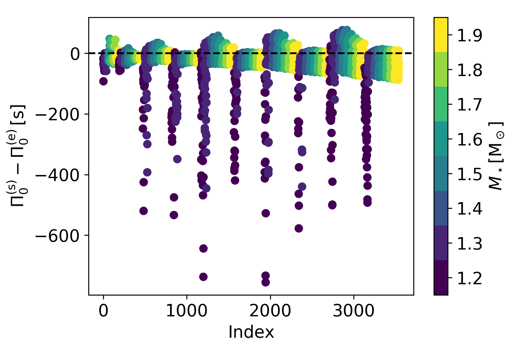
taking into account the variance across the grid, where $\bar{Y}$ is the mean value of $\bm{Y}$ in the grid. We choose eight benchmark $\gamma$ Dor models; a young low-mass star, an old low-mass star, a young high-mass star and an old high-mass star, with $Z=0.014$, $X_{\rm ini}=0.71$, $\alpha_{\rm ov}(f_{\rm ov})=0.15(0.015)$ and $D_{\rm mix}=$1.0\text{\,}{\mathrm{cm}}^{2}\text{\,}{\mathrm{s}}^{-1}$$, all for both overshooting prescriptions. In Table 5 we list the maximum likelihood estimate (MLE) from using an incorrect overshooting prescription for each of these eight benchmark models. For all of these models, the resulting $\bm{\theta}_{0}$ from fitting $(\Pi_{0},T_{\rm eff},\log g)$ does not change drastically, compared to the step size of the grids for $M_{\star}$ and $X_{\rm c}^{\prime}$. The grids contain too few points in the other parameters to draw a conclusion on how robust the MLE is for these parameters. However, even though there is scatter in $\alpha_{\rm ov}/f_{\rm ov}$, $D_{\rm mix}$, $Z$ and $X_{\rm ini}$, similar masses and age-proxies are found.

Furthermore, we note that for $\alpha_{\rm ov}=10f_{\rm ov}$, the MLE agrees well with the input parameters (see Fig. 5). This scaling with a factor 10 between $\alpha_{\rm ov}$ and $f_{\rm ov}$ is a commonly used rule-of-thumb when comparing step overshoot and exponential overshoot. In Fig. 5, the difference in $\Pi_{0}$ is plotted between two models, each from a different grid, that have the same parameters ($X_{\rm c}^{\prime}$ within 0.001) where $\alpha_{\rm ov}=10f_{\rm ov}$. This scaling rule does give similar values for $\Pi_{0}$ within the parameter space of $\gamma$ Dor stars, compared to typical uncertainties on this seismic parameter, as the difference is less than $60\text{\,}\mathrm{s}$ for masses above 1.4 M_⊙. The deviation between the two grids at the lower masses is a result from the fact that this factor 10 is not exact and also mass dependent (11.36 $\pm$ 0.22 was found by Claret & Torres, 2017). We stress that our inability to distinguish between step and exponential overshooting from the MLE is due to the coarseness of the grids (Table 1), as this determines how well $\bm{Y}^{\rm(obs)}$ can be matched in the other grid. This can be seen in the last three columns of Table 5.

Figure 5: Difference between $\Pi_{0}$ in the step overshoot grid ($\Pi_{0}^{\rm(s)}$) and the exponential overshoot grid ($\Pi_{0}^{\rm(e)}$), for pairs of models with the same parameters $M_{\star}$, $X_{\rm c}^{\prime}$, $D_{\rm mix}$, $Z$, $X_{\rm ini}$, varied across the grid. An $\alpha_{\rm ov}$ in one grid corresponds to $10f_{\rm ov}$ in the other grid. The pairs of models are equally distributed across both grids and are arbitrarily labelled from 1 to 3541. When $M_{\star}\geq 1.4$ M_⊙ the maximum difference is comparable with a typical observational uncertainty on $\Pi_{0}$. For visual aid, a dashed line is plotted at zero difference.

	$M_{\star}\,$[ M⊙ ]	$X_{\rm c}^{\prime}$	$\alpha_{\rm ov}$	$f_{\rm ov}$	$D_{\rm mix}\,$[cm-2s-1]	$Z$	$X_{\rm ini}$	$\Pi_{0}\,$[s]	$T_{\rm eff}\,$[K]	$\log g$
BM	1.30	0.90	0.150	-	1.0	0.014	0.71	4327	6669	4.33
GRID	1.35	0.92	-	0.0075	10.0	0.014	0.73	4330	6678	4.33
BM	1.30	0.90	-	0.0150	1.0	0.014	0.71	4352	6669	4.33
GRID	1.25	0.88	0.225	-	1.0	0.014	0.69	4343	6657	4.33
BM	1.30	0.10	0.150	-	1.0	0.014	0.71	3140	6158	4.04
GRID	1.35	0.10	-	0.0010	10.0	0.018	0.69	3147	6186	4.04
BM	1.30	0.10	-	0.0150	1.0	0.014	0.71	3182	6104	4.01
GRID	1.25	0.10	0.225	-	1.0	0.014	0.69	3179	6099	4.02
BM	2.00	0.90	0.150	-	1.0	0.014	0.71	5551	9217	4.29
GRID	2.00	0.90	-	0.0150	0.1	0.014	0.71	5535	9216	4.29
BM	2.00	0.90	-	0.0150	1.0	0.014	0.71	5531	9218	4.29
GRID	2.00	0.90	0.150	-	1.0	0.014	0.71	5551	9217	4.29
BM	2.00	0.10	0.150	-	1.0	0.014	0.71	4172	7100	3.69
GRID	1.80	0.17	-	0.0225	10.0	0.010	0.71	4166	7088	3.69
BM	2.00	0.10	-	0.0150	1.0	0.014	0.71	4210	6957	3.64
GRID	1.90	0.14	0.300	-	1.0	0.010	0.73	4221	6979	3.63

Table 5: The MLEs for eight different benchmark models (BM) using a grid with the incorrect overshooting prescription, i.e., step overshoot models are fitted to an exponential overshoot grid and vice versa.

4 Parameter estimation from $\Pi_{0}$, $T_{\rm eff}$, and $\log g$

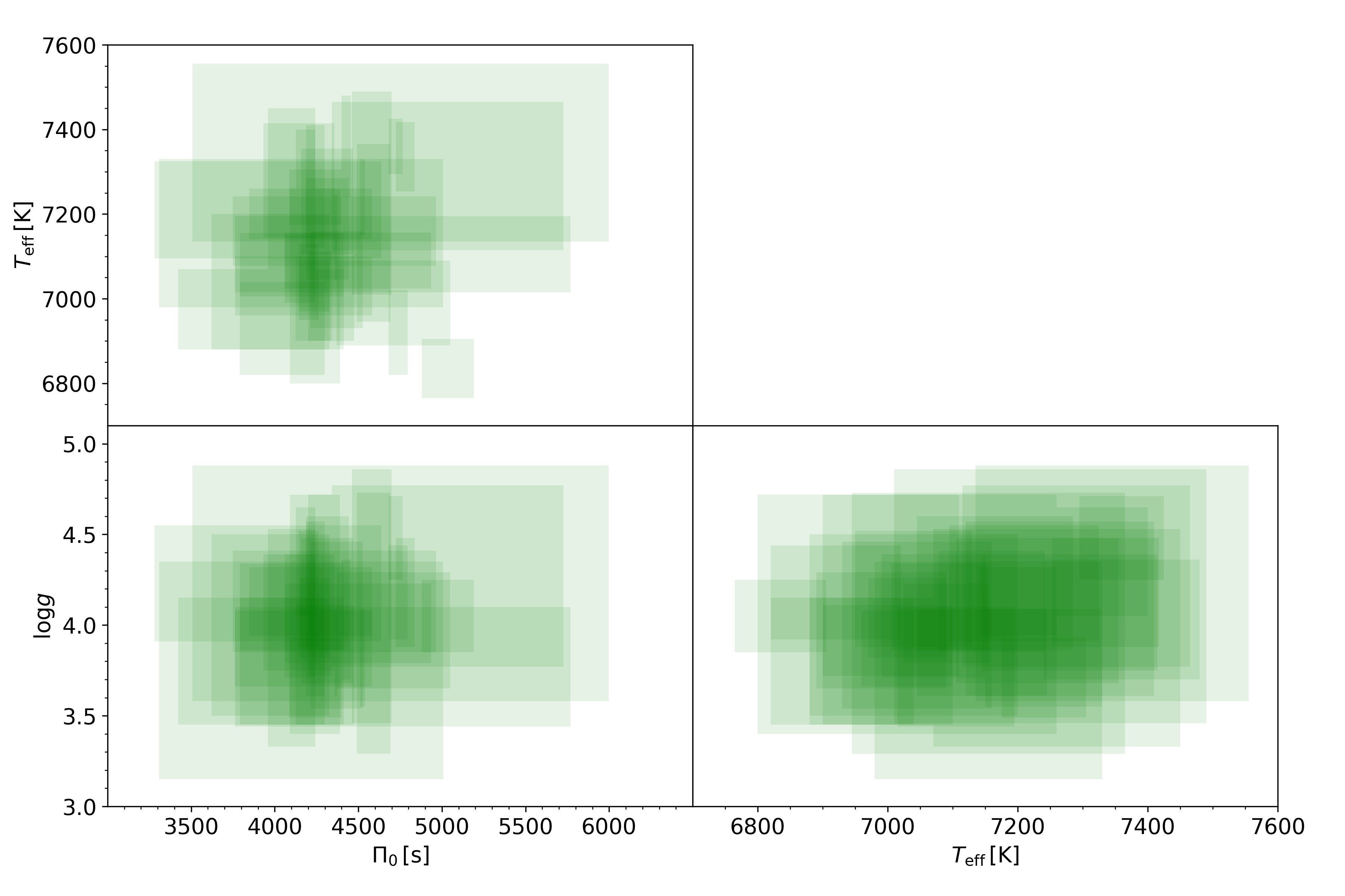
We aim to test the feasibility of estimating (some of) the six parameters in the two grids for all $\gamma$ Dor stars in the sample of Van Reeth et al. (2016) with $\Pi_{0}$ deduced from prograde dipole modes in an automated way. We recall that these measured values of $\Pi_{0}$ were derived along with estimation of the near-core rotation frequency (Van Reeth et al., 2016; Van Reeth et al., 2018). Our aim is to test if $\Pi_{0}$, along with spectroscopic measurements of $T_{\rm eff}$ and $\log g$ are sufficient to estimate $M_{\star}$, $X_{\rm c}^{\prime}$, $\alpha_{\rm ov}/f_{\rm ov}$, and possibly $Z$, $X_{\rm ini}$ and/or $D_{\rm mix}$ from an ensemble of $\gamma$ Dor stars (see Fig. 6, illustrating the 2D projected 1$\sigma$ errors on the observed parameters of each star). We use an automated grid-based approach, keeping in mind the uncertainties of individual theoretically computed g-mode frequencies due to unknown aspects of the input physics of the stellar models, as assessed by Aerts et al. (2018). These authors describe a new method for forward seismic modelling, where the correlation between the observables is taken into account. This method is based on the Mahalanobis distance which is defined in our 3D case as

$$D_{{\rm M},j}=\left(\bm{Y}_{j}^{(\rm th)}-\bm{Y}^{(\rm obs)}\right)^{\top}\left(\bm{\Lambda}+\bm{V}\right)^{-1}\left(\bm{Y}_{j}^{(\rm th)}-\bm{Y}^{(\rm obs)}\right).$$ (18)

The matrix $\bm{\Lambda}$ = diag$(\sigma_{\Pi_{0}}^{2},\sigma_{T_{\rm eff}}^{2},\sigma_{\log g}^{2})$ takes the uncertainties of the observed quantities into account and the (co-)variance matrix $\bm{V}$ is computed according Eq. (17) for both grids.

Figure 6: 2D projected 1$\sigma$ error boxes of the observable ($\Pi_{0}$, $T_{\rm eff}$, $\log g$) for the 37 stars in our sample for which spectroscopic measurements are available.

We first get MLEs for all stars in our sample for which spectroscopic data is available by minimizing the Mahalanobis distance across each of the grids. As has already been demonstrated with the statistical models presented in Section 2, some parameters are more strongly correlated with the observables than others. We therefore assess whether it is possible to reduce the dimension of our forward modelling problem from a principal component analysis (PCA). For each star, the best 10 per cent of the models is selected and the basis of this 6D solution space is redefined in terms of its principal components (PCs). These PCs are the eigenvectors of the correlation matrix and the corresponding normalised eigenvalues give the percentages of the total variance that is captured by each PC. As a rule-of-thumb, the number of PCs selected is the number of PCs which is needed to describe at least 80 per cent of the total variance (Jolliffe, 2002). In this way, we find that four PCs are sufficient for all the 37 stars in the sample.

The PCs that can be dropped are predominantly connected with $D_{\rm mix}$ and $X_{\rm ini}$. Therefore, we wish to remove these two parameters from the grid to reduce the dimensionality, by fixing a value for them. In order to assign the most appropriate fixed value, we consider each of the six combinations of these two parameters available in the grids and determine the MLE for all stars in our sample. For the four estimated parameters, the average standard deviations between these six MLEs is found to be $\langle\sigma_{M_{\star}}\rangle=0.06$ M_⊙, $\langle\sigma_{X_{\rm c}}\rangle=0.02$, $\langle\sigma_{\alpha_{\rm ov}}\rangle=0.061$ and $\langle\sigma_{Z}\rangle=0.001$, for step overshoot. For exponential overshoot, $\langle\sigma_{M_{\star}}\rangle=0.06$ M_⊙, $\langle\sigma_{X_{\rm c}}\rangle=0.03$, $\langle\sigma_{f_{\rm ov}}\rangle=0.062$ and $\langle\sigma_{Z}\rangle=0.001$. Based on these values, we argue that $D_{\rm mix}$ and $X_{\rm ini}$ can be set to the fixed values $1.0\text{\,}{\mathrm{cm}}^{2}\text{\,}{\mathrm{s}}^{-1}$ and 0.71, respectively.

The results of the parameters estimations from MLE are listed in Table 6 for both overshooting prescriptions. The corresponding fractional mass and fractional radius of the convective core of the best model are also listed. For $M_{\star}$, $X_{\rm c}^{\prime}$, $M_{\rm cc}^{\prime}$ and $R_{\rm cc}^{\prime}$ (fractional mass and radius of the convective core), the grid is comprised of a sufficiently large number of points to make a comparison. However, for these parameters there is no obvious discrepancy reported between the two overshooting prescriptions for any given star.

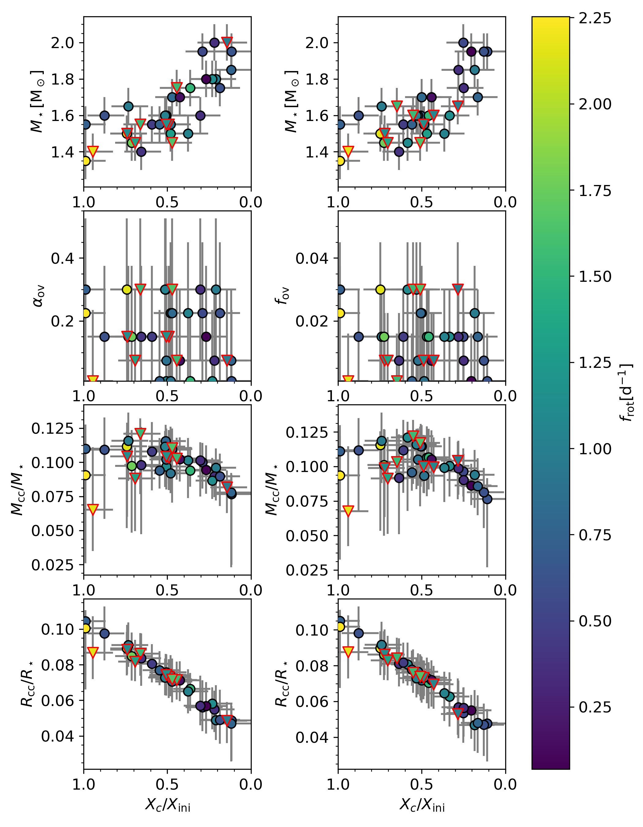
The relation between the near-core rotation frequency $f_{\rm rot}$ and the evolutionary state of the stars in our sample has previously been investigated by Aerts et al. (2017, their fig. 1), where the spectroscopic $\log g$ was used as a proxy for the evolutionary stage. In Fig. 7, $\log g$ is replaced by the MLE of $X_{\rm c}^{\prime}$ for both overshooting prescriptions. We colour-code for the measured near-core rotation rate, for which the relative uncertainty is typically a few per cent. From these more precise estimates of the proxy for stellar age, the data reveal that the cores of intermediate-mass A and F stars spin down as the stars evolve.

Ouazzani et al. (2018) report that faster rotators are less massive and younger than the slow rotators. This is consistent with our findings that the two aforementioned faster rotating near-ZAMS stars are less massive than the slower rotating stars with roughly the same $X_{\rm c}^{\prime}$, as shown in the top row of Fig. 7. As the $\gamma$ Dor instability region is relatively small (Bouabid et al., 2013), it is possible for stars to be born on the ZAMS outside of the instability region and later evolve into it, and vice versa. Therefore, it is expected that high-mass $\gamma$ Dor stars are slow rotators since they are closer to the TAMS than low-mass stars. Yet, the fact we do not observe any evolved fast rotators might also be caused by an observational selection bias, because the structure of a TAMS star combined with fast rotation creates a dense, and typically unresolvable spectrum of pulsation modes (e.g., Buysschaert et al. 2018). Nevertheless, the fact that the fastest rotators in our sample are all found to be relatively young suggests that the transport of angular momentum from the core to the envelope must be efficient already early on in the stellar evolution. Given that the convective core size decreases as the star evolves (cf., Fig. 2), our findings suggest that the efficiency of angular momentum transport is somehow connected to the convective core, as already hinted at by Aerts et al. (2019). So far, the individual roles of gravito-inertial and Rossby modes in angular momentum transport remain unclear. As can been seen in Fig. 7, we find stars with observed Rossby modes (plotted as triangles) to be situated across the main sequence, except close to the TAMS.

In the second row of Fig. 7 we plot the MLEs of the overshoot versus $X_{\rm c}^{\prime}$ and colour-code by the rotation rate to investigate if a higher overshooting estimate corresponds with faster rotation at the interface of the convective core and the radiative envelope. For both overshooting prescriptions, the MLE of the overshooting shows no correlation between the amount of core overshooting mixing and the near-core rotation frequency. This result is complementary to the conclusion by Aerts et al. (2014) that the surface nitrogen excess of a sample of OB stars, which demands efficient mixing in the stellar envelope, is not correlated with their surface rotation frequency but rather with the frequency of the pressure mode with dominant amplitude. Taking the results of both studies together suggest that core boundary mixing may have various causes, such as rotational mixing (e.g., Brott et al., 2011) or pulsational mixing induced by waves (e.g., Rogers & McElwaine, 2017), but that its shape remains to be determined. In our modelling, these various kinds of mixing were coded with two functional shapes with a free parameter, i.e., as core overshooting and envelope mixing, without specifying the underlying physical phenomenon. The estimated parameters of these two prescriptions, $f_{\rm ov}$ (or $\alpha_{\rm ov}$) and $D_{\rm mix}$, do not reveal what causes the near-core mixing, but only provide a rough level of mixing required to explain the g-mode behaviour. We find that we cannot pinpoint particular values for our ensemble of stars, suggesting that different physical phenomena may lie at the basis of the overall level of near-core mixing. This is in agreement with the findings for the more massive B-type pulsators (Aerts, 2015).

In the last two rows of Fig. 7 the fractional mass and radius of the convective core are placed on the ordinate axis. We see that estimation of the convective core mass and size is well achieved, despite the absence of predictive power for the core overshoot parameter. This is the same conclusion as found by Johnston et al. (2019) for three gravity-mode pulsators in close binaries and points to a strong probing power of dipole gravity modes (through $\Pi_{0}$) to assess convective core properties. When we compare the four stars closest to ZAMS, we notice that the two stars with a lower $f_{\rm rot}$ have more massive and larger convective cores than the two faster rotating stars. However, the overlapping confidence intervals do not allow us to claim a significant dichotomy with certainty.

5 Confidence intervals from ensemble modelling

Determining uncertainty intervals from the distributions of the Mahalanobis distance of each individual star (Aerts et al. 2018; problem 1) is not meaningful because of the large span of these intervals in the grids. This should not come as a surprise, given that one is then determining an estimator based on a single star, i.e., a sample of size one. A convenient way to deal with this consists of considering the sample of $S=37$ as an ensemble. This is taken to mean a collection of stars that, while having star-specific characteristics and hence parameters $\mbox{\boldmath$\theta$}_{s}$, makes up a sufficiently ‘natural’ family fulfilling the same underlying theory of stellar structure.

Evidently, when a sample of size $S$ is available, the average of the parameters $\mbox{\boldmath$\theta$}_{s}$, say $\theta$, can be estimated much more precisely than the parameter of an individual star. If we think of a given star parameter $\mbox{\boldmath$\theta$}_{s}$ as being decomposed into $\mbox{\boldmath$\theta$}_{s}=\mbox{\boldmath$\theta$}+\mbox{\boldmath$t$}_{s}$, with $\mbox{\boldmath$t$}_{s}$ the star-specific deviation around $\theta$, then we can use the precision of $\widehat{\mbox{\boldmath$\theta$}}$, the MLE, as a measure of precision for the entire sample. Precisely, we write the likelihood for the entire sample as

$$\begin{split}L=&\prod_{s=1}^{S}\frac{1}{(2\pi)^{P/2}|V_{s}|^{-1/2}}\times\\ &\exp\left\{-\frac{1}{2}\left[\mbox{\boldmath$Y$}_{s}(\mbox{\boldmath$\theta$}_{s})-\mbox{\boldmath$Y$}_{s}^{\ast}\right]^{\top}V_{s}^{-1}\left[\mbox{\boldmath$Y$}_{s}(\mbox{\boldmath$\theta$}_{s})-\mbox{\boldmath$Y$}_{s}^{\ast}\right]\right\},\\ \end{split}$$ (19)

with $P=\dim(\mbox{\boldmath$Y$})$. In our application, $S=37$ and $P=3$. The kernel of the log-likelihood is

$$\ell=-\frac{1}{2}\sum_{s=1}^{S}\ln|V_{s}|-\frac{1}{2}\sum_{s=1}^{S}\left[\mbox{\boldmath$Y$}_{s}(\mbox{\boldmath$\theta$}_{s})-\mbox{\boldmath$Y$}_{s}^{\ast}\right]^{\top}V_{s}^{-1}\left[\mbox{\boldmath$Y$}_{s}(\mbox{\boldmath$\theta$}_{s})-\mbox{\boldmath$Y$}_{s}^{\ast}\right].$$ (20)

Consider now the deviance function for the $k$th component of $\theta$

$$D(h) = -\sum_{s=1}^{S}\left[\mbox{\boldmath$Y$}_{s}(\mbox{\boldmath$\theta$}_{s})-\mbox{\boldmath$Y$}_{s}^{\ast}\right]^{\top}V_{s}^{-1}\left[\mbox{\boldmath$Y$}_{s}(\mbox{\boldmath$\theta$}_{s})-\mbox{\boldmath$Y$}_{s}^{\ast}\right]$$

$$+\sum_{s=1}^{S}\left[\mbox{\boldmath$Y$}_{s}(\mbox{\boldmath$\theta$}^{(k,h)}_{s})-\mbox{\boldmath$Y$}_{s}^{\ast}\right]^{\top}V_{s}^{-1}\left[\mbox{\boldmath$Y$}_{s}(\mbox{\boldmath$\theta$}^{(k,h)}_{s})-\mbox{\boldmath$Y$}_{s}^{\ast}\right],$$

with $\mbox{\boldmath$\theta$}^{(k,h)}_{s}=\mbox{\boldmath$\theta$}_{s}$, except in the $k$th component, where we put $\theta^{(k,h)}_{s,k}=\theta_{s,k}+h$, where $h$ is a (discrete) perturbation. We then search for both the negative and positive $h$ values, say $h_{L}$ and $h_{U}$, that satisfy $D(h_{L})=D(h_{U})=3.84$ which is the critical value of the $\chi^{2}_{1}$ distribution. When making use of a sufficiently fine grid, those grid points can be chosen that satisfy the above requirement sufficiently well. The corresponding confidence interval is:

$$[\theta_{s,k}+h_{L};\theta_{s,k}+h_{U}].$$

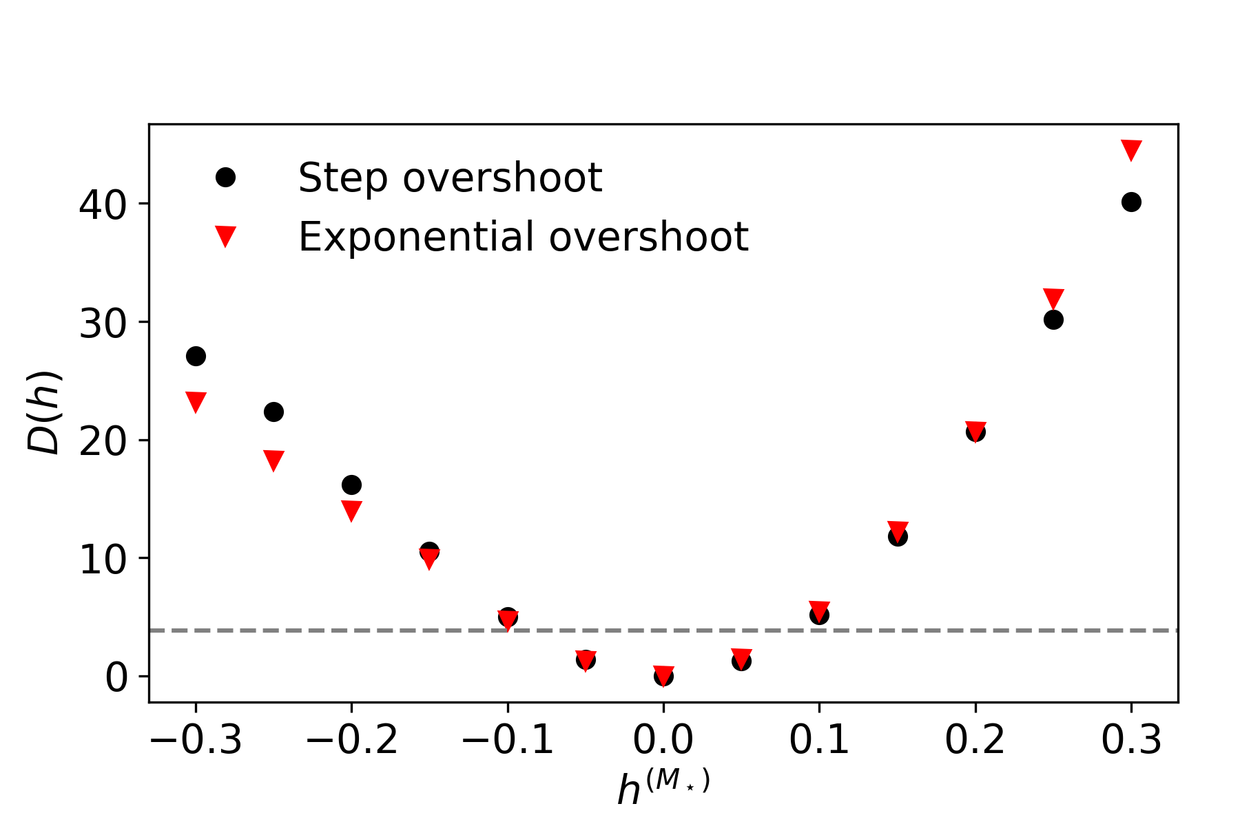
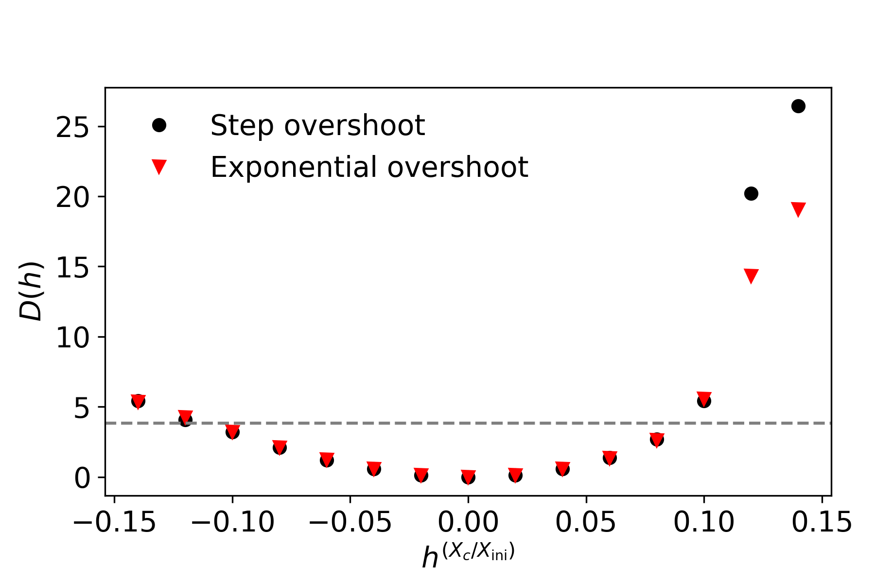
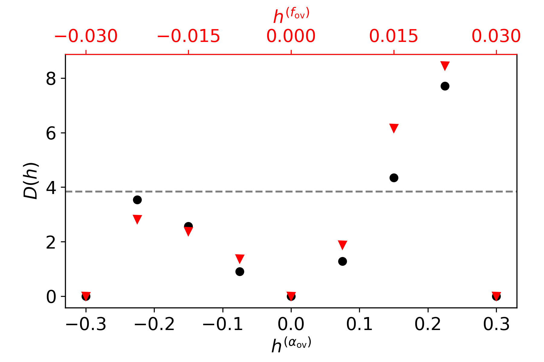
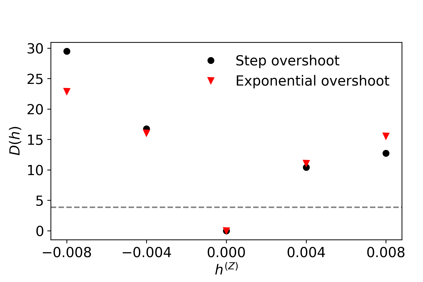
Because the likelihood ratio is not based on a quadratic approximation, the interval is not necessarily symmetric, but it will be more symmetric in larger samples. In Appendix B, the deviance function is plotted as a function of the four parameters we have estimated. The grid is quite coarse for overshoot and $Z$ to properly sample $D(h)$, hence we stay on the conservative side and pick the values of $h_{L}$ and $h_{U}$ as the smallest discrete values for which the deviance function is larger than 3.84. For $X_{\rm c}^{\prime}$, the confidence interval may, statistically seen, contain unphysical values and therefore we truncate the interval at the edge of the grid. The confidence interval of the overshoot is only truncated at the lower edge of the grid. For both overshoot grids we were not able to determine $h_{L}$ for our ensemble, therefore the lower limit on $\alpha_{\rm ov}$ and on $f_{\rm ov}$ is always the lowest value in the respective grid. In Appendix B, the sampling of $D(h)$ is shown for the four parameters that estimated from the the MLE. This yields uncertainties of 0.1 M_⊙ on $M_{\star}$, 0.004 on $Z$ (in these cases symmetric), all rounded to the nearest step in the respective grids and 0.12 and 0.10 on $X_{\rm c}^{\prime}$ for the lower and upper uncertainties, respectively. The uncertainties on $M_{\rm cc}^{\prime}$ and $R_{\rm cc}^{\prime}$ are defined as the minimum and maximum values found in the models that lay within the confidence intervals of the estimated parameters.

Figure 7: Top to bottom: MLEs for $X_{\rm c}^{\prime}$ versus mass, overshoot, convective core mass and convective core radius, colour-coded by the measured near-core rotation frequency from Van Reeth et al. (2016), for all 37 stars in our sample. Left column: Step overshoot. Right column: Exponential overshoot. Stars that have observed Rossby modes in addition to gravito-inertial prograde dipole modes are plotted as triangles.

6 Discussion & Conclusions

In this paper we have explored the power of $\Pi_{0}$ estimated from prograde dipole gravito-inertial modes and in some cases also from Rossby modes, combined with spectroscopic measurements of the effective temperature and surface gravity to perform asteroseismic modelling of $\gamma$ Dor stars, which have a well-developed convective core. We devised recipes relating the most important fundamental stellar parameters to these three observables, from multivariate linear regression, and have shown that these linear recipes have a proper predicting capacity with respect to the measurement uncertainties. The recipes are advantageous in the forward modelling of $\gamma$ Dor stars, as they imply a huge decrease in computation time while still providing good constraints for the stellar parameters in the high-dimensional parameter space. The method of backward selection based on the BIC reveals that, among the mass, metallicity, central and initial hydrogen mass fraction, mass and size of the convective core and the amount of mixing in the radiative zone, only the latter can be ignored in the linear recipes. Previously it was found that fitting frequencies of individual trapped gravity modes does require extra mixing in the radiative envelope (Moravveji et al., 2015, 2016; Schmid & Aerts, 2016).

The forward modelling of $\gamma$ Dor stars is a cumbersome task if the aim is to achieve stellar parameters with a relative precision of 10 per cent or better. This can only be reached when $\Pi_{0}$, $T_{\rm eff}$, and $\log g$ are measured with high precision. This problem is illustrated in Fig. 6 where the 2D projected 1$\sigma$ error boxes for $\bm{Y}^{\rm(obs)}$ are plotted for all 37 stars in our sample. Even though we use high-precision spectroscopy here, the error boxes are still relatively large due to the correlated nature of the three observables.

This work contains the first asteroseismic forward modelling of $\gamma$ Dor stars as an ensemble, using the Mahalanobis distance as described in Aerts et al. (2018). With this method, we assume the sample stars to adhere to a single underlying stellar evolution theory and that each star with its own parameters can be seen as a deviation of an average star in the ensemble to derive meaningful uncertainties to go along with the MLEs of $M_{\star}$, $X_{\rm c}^{\prime}$, $\alpha_{\rm ov}/f_{\rm ov}$, $Z$, as well as the mass and radius of the convective core for the 37 $\gamma$ Dor stars in our sample. From PCA it was concluded that the dimensionality of this problem could be reduced to a 4D problem when fitting $(\Pi_{0},T_{\rm eff},\log g)$, by fixing $X_{\rm ini}$ and $D_{\rm mix}$. For $M_{\star}$ and $X_{\rm c}^{\prime}$ we find in general consistent results between a step and an exponential overshooting prescription.

We have demonstrated that linear statistical models are able to capture the correlated nature of the three observables $\Pi_{0}$, $T_{\rm eff}$ and $\log g$, and the fundamental stellar parameters, up to the level of the measurement uncertainties. This finding allows us to use recipes rather than having to compute dense stellar model grids when fitting the observables $(\Pi_{0},T_{\rm eff},\log g)$ for future applications to additional $\gamma\,$Dor stars.

Future work will involve the addition of $X_{\rm ini}$, $D_{\rm mix}$ and $\alpha_{\rm MLT}$ in the modelling of the morphology of the period spacing patterns for all $\gamma\,$Dor stars with suitable mode detection and spectroscopy, rather than just $\Pi_{0}$. Especially the mixing profile in the radiative zone cannot be constrained with the observables in this paper, but does have a large effect on the morphology of the period spacing pattern. The dips in the pattern caused by mode-trapping decrease when the mixing efficiency increases as this process washes out the chemical gradient and therefore reduces the effect of mode trapping, as shown in B-type stars (Moravveji et al., 2015). As computing the individual theoretical frequencies is a more computationally demanding exercise, the MLEs of $M_{\star}$, $X_{\rm c}^{\prime}$, $\alpha_{\rm ov}/f_{\rm ov}$ and $Z$ presented in this paper provide a starting point for refined modelling to estimate $D_{\rm mix}(r)$. The ongoing NASA TESS (Ricker et al., 2015) and upcoming ESA PLATO (Rauer et al., 2014) space missions will deliver many new g-mode pulsators covering a mass range of 1.2 to $\sim$20 M_⊙. Therefore, the similar analysis of potentially thousands of new g-mode pulsators and its extension to include binary star information (e.g., Johnston et al. 2019) with the next generation of space telescopes will provide an improved insight of stellar structure and evolution of stars with convective cores across the HR diagram.

Appendix A Mode cavities in a typical $\gamma$ Dor stellar model

Here, we show an example of the mode cavities of the gravity (g) modes and pressure (p) modes in a $\gamma$ Dor star.

Figure 8: Mode cavities of the g modes (green, $n_{\rm pg}\,\in\,[-50,-1]$) and p modes (grey, $n_{\rm pg}\,\in\,[1,4]$) in a 1.8 M_⊙ star at $X_{\rm c}^{\prime}=0.4$ for $(l,m)=(1,1)$. The mode frequencies $\omega_{n11}$ were computed with GYRE, adopting the TAR for a uniform rotation at 20 per cent of the critical rotation velocity in the Roche formalism. The dashed lines are placed at the mode frequencies and the black dots mark the position of the radial nodes of each mode. The solid black line is the Brunt-Väisälä frequency, the dotted line is the dipole-mode Lamb frequency $S_{l=1}$. The effect of rotation is only taken into account in the computation of the mode frequencies and not in the equilibrium model (Aerts et al., 2018, for a thorough justification of such an approach in gravity-mode asteroseismology).

Appendix B Deviance functions

Below we show the behaviour of the deviance functions used for determining the confidence intervals from ensemble modelling as described in Section 5.

Figure 9: deviance function $D(h)$, where $h$ is a ‘perturbation’ in $M_{\star}$ of the best model. The dashed grey line at 3.84 indicates the critical value of the $\chi_{1}^{2}$ distribution.

Figure 10: Same as Fig. 9, but for $X_{\rm c}^{\prime}$.

Figure 11: Same as Fig. 9, but for overshoot.

 

Figure 12: Same as Fig. 9, but for $Z$.

Appendix C Influence of the mixing length parameter

In this appendix we present the differences in the theoretical prediction of $\Pi_{0}$, $T_{\rm eff}$, and $\log g$ caused by the use of a different value of $\alpha_{\rm MLT}$ in the computation of stellar models for a high-mass and low-mass $\gamma$ Dor star.

Figure 13: Evolution of $\Pi_{0}$ for different values of the mixing length parameter $\alpha_{\rm MLT}$. The average uncertainty on $\Pi_{0}$ (in grey) for the stars in our sample is also plotted for comparison.

Figure 14: Same as Fig. 13, but for $T_{\rm eff}$.

Figure 15: Same as Fig. 13, but for $\log g$.

Appendix D Maximum likelihood estimates of the stellar parameters

Below we present the maximum likelihood estimates described in Sections 4 and 5 for each of the five stellar parameters estimated for all the 37 stars in our sample, along with the observed value of $\Pi_{0}$.

KIC ID	$\Pi_{0}^{\rm(obs)}$[s]	$M_{\star}[M_{\odot}]$	$X_{\rm c}^{\prime}$	$\alpha_{\rm ov}$	$f_{\rm ov}$	$Z$	$M_{\rm cc}/M_{\star}$	$R_{\rm cc}/R_{\star}$
KIC2710594	4301 $\begin{subarray}{c}+175\\ -170\end{subarray}$	2.00	0.14 $\begin{subarray}{c}+0.10\\ -0.12\end{subarray}$	0.075 $\begin{subarray}{c}+0.150\\ -0.065\end{subarray}$	-	0.018	0.082 $\begin{subarray}{c}+0.013\\ -0.019\end{subarray}$	0.049 $\begin{subarray}{c}+0.011\\ -0.013\end{subarray}$
		1.65	0.29 $\begin{subarray}{c}+0.10\\ -0.12\end{subarray}$	-	0.0300 $\begin{subarray}{c}+0.0150\\ -0.0290\end{subarray}$	0.010	0.104 $\begin{subarray}{c}+0.014\\ -0.028\end{subarray}$	0.053 $\begin{subarray}{c}+0.020\\ -0.012\end{subarray}$
KIC3448365	4237 $\begin{subarray}{c}+91\\ -91\end{subarray}$	1.55	0.49 $\begin{subarray}{c}+0.10\\ -0.12\end{subarray}$	0.150 $\begin{subarray}{c}+0.150\\ -0.140\end{subarray}$	-	0.014	0.103 $\begin{subarray}{c}+0.020\\ -0.024\end{subarray}$	0.073 $\begin{subarray}{c}+0.010\\ -0.012\end{subarray}$
		1.60	0.43 $\begin{subarray}{c}+0.10\\ -0.12\end{subarray}$	-	0.0075 $\begin{subarray}{c}+0.0150\\ -0.0065\end{subarray}$	0.014	0.100 $\begin{subarray}{c}+0.021\\ -0.018\end{subarray}$	0.070 $\begin{subarray}{c}+0.010\\ -0.014\end{subarray}$
KIC4846809	4144 $\begin{subarray}{c}+198\\ -212\end{subarray}$	1.50	0.48 $\begin{subarray}{c}+0.10\\ -0.12\end{subarray}$	0.225 $\begin{subarray}{c}+0.150\\ -0.215\end{subarray}$	-	0.010	0.109 $\begin{subarray}{c}+0.017\\ -0.032\end{subarray}$	0.074 $\begin{subarray}{c}+0.011\\ -0.012\end{subarray}$
		1.50	0.47 $\begin{subarray}{c}+0.10\\ -0.12\end{subarray}$	-	0.0150 $\begin{subarray}{c}+0.0150\\ -0.0140\end{subarray}$	0.010	0.106 $\begin{subarray}{c}+0.023\\ -0.028\end{subarray}$	0.073 $\begin{subarray}{c}+0.011\\ -0.014\end{subarray}$
KIC5114382	4315 $\begin{subarray}{c}+129\\ -122\end{subarray}$	1.50	0.74 $\begin{subarray}{c}+0.10\\ -0.12\end{subarray}$	0.150 $\begin{subarray}{c}+0.150\\ -0.140\end{subarray}$	-	0.014	0.104 $\begin{subarray}{c}+0.025\\ -0.044\end{subarray}$	0.088 $\begin{subarray}{c}+0.014\\ -0.014\end{subarray}$
		1.50	0.72 $\begin{subarray}{c}+0.10\\ -0.12\end{subarray}$	-	0.0075 $\begin{subarray}{c}+0.0150\\ -0.0065\end{subarray}$	0.014	0.099 $\begin{subarray}{c}+0.028\\ -0.035\end{subarray}$	0.086 $\begin{subarray}{c}+0.014\\ -0.011\end{subarray}$
KIC5522154	4738 $\begin{subarray}{c}+57\\ -42\end{subarray}$	1.50	0.74 $\begin{subarray}{c}+0.10\\ -0.12\end{subarray}$	0.300 $\begin{subarray}{c}+0.150\\ -0.290\end{subarray}$	-	0.018	0.112 $\begin{subarray}{c}+0.011\\ -0.060\end{subarray}$	0.089 $\begin{subarray}{c}+0.009\\ -0.015\end{subarray}$
		1.50	0.75 $\begin{subarray}{c}+0.10\\ -0.12\end{subarray}$	-	0.0300 $\begin{subarray}{c}+0.0150\\ -0.0290\end{subarray}$	0.018	0.116 $\begin{subarray}{c}+0.010\\ -0.062\end{subarray}$	0.090 $\begin{subarray}{c}+0.010\\ -0.015\end{subarray}$
KIC5708550	4709 $\begin{subarray}{c}+339\\ -311\end{subarray}$	1.70	0.47 $\begin{subarray}{c}+0.10\\ -0.12\end{subarray}$	0.225 $\begin{subarray}{c}+0.150\\ -0.215\end{subarray}$	-	0.018	0.110 $\begin{subarray}{c}+0.015\\ -0.023\end{subarray}$	0.071 $\begin{subarray}{c}+0.012\\ -0.012\end{subarray}$
		1.70	0.50 $\begin{subarray}{c}+0.10\\ -0.12\end{subarray}$	-	0.0225 $\begin{subarray}{c}+0.0150\\ -0.0215\end{subarray}$	0.018	0.115 $\begin{subarray}{c}+0.015\\ -0.026\end{subarray}$	0.072 $\begin{subarray}{c}+0.013\\ -0.013\end{subarray}$
KIC5788623	3960 $\begin{subarray}{c}+679\\ -622\end{subarray}$	1.40	0.66 $\begin{subarray}{c}+0.10\\ -0.12\end{subarray}$	0.150 $\begin{subarray}{c}+0.150\\ -0.140\end{subarray}$	-	0.010	0.098 $\begin{subarray}{c}+0.028\\ -0.051\end{subarray}$	0.084 $\begin{subarray}{c}+0.014\\ -0.016\end{subarray}$
		1.40	0.64 $\begin{subarray}{c}+0.10\\ -0.12\end{subarray}$	-	0.0075 $\begin{subarray}{c}+0.0150\\ -0.0065\end{subarray}$	0.010	0.092 $\begin{subarray}{c}+0.032\\ -0.041\end{subarray}$	0.081 $\begin{subarray}{c}+0.014\\ -0.013\end{subarray}$
KIC6468146	4243 $\begin{subarray}{c}+156\\ -156\end{subarray}$	1.80	0.21 $\begin{subarray}{c}+0.10\\ -0.12\end{subarray}$	0.300 $\begin{subarray}{c}+0.150\\ -0.290\end{subarray}$	-	0.010	0.096 $\begin{subarray}{c}+0.014\\ -0.024\end{subarray}$	0.049 $\begin{subarray}{c}+0.020\\ -0.011\end{subarray}$
		1.85	0.18 $\begin{subarray}{c}+0.10\\ -0.12\end{subarray}$	-	0.0225 $\begin{subarray}{c}+0.0150\\ -0.0215\end{subarray}$	0.010	0.094 $\begin{subarray}{c}+0.018\\ -0.024\end{subarray}$	0.047 $\begin{subarray}{c}+0.019\\ -0.015\end{subarray}$
KIC6468987	4591 $\begin{subarray}{c}+100\\ -95\end{subarray}$	1.75	0.44 $\begin{subarray}{c}+0.10\\ -0.12\end{subarray}$	0.075 $\begin{subarray}{c}+0.150\\ -0.065\end{subarray}$	-	0.018	0.103 $\begin{subarray}{c}+0.015\\ -0.016\end{subarray}$	0.071 $\begin{subarray}{c}+0.010\\ -0.011\end{subarray}$
		1.60	0.55 $\begin{subarray}{c}+0.10\\ -0.12\end{subarray}$	-	0.0300 $\begin{subarray}{c}+0.0150\\ -0.0290\end{subarray}$	0.014	0.122 $\begin{subarray}{c}+0.012\\ -0.035\end{subarray}$	0.076 $\begin{subarray}{c}+0.013\\ -0.011\end{subarray}$
KIC6678174	4766 $\begin{subarray}{c}+1004\\ -877\end{subarray}$	1.95	0.29 $\begin{subarray}{c}+0.10\\ -0.12\end{subarray}$	0.225 $\begin{subarray}{c}+0.150\\ -0.215\end{subarray}$	-	0.018	0.100 $\begin{subarray}{c}+0.014\\ -0.019\end{subarray}$	0.056 $\begin{subarray}{c}+0.015\\ -0.013\end{subarray}$
		2.00	0.25 $\begin{subarray}{c}+0.10\\ -0.12\end{subarray}$	-	0.0150 $\begin{subarray}{c}+0.0150\\ -0.0140\end{subarray}$	0.018	0.096 $\begin{subarray}{c}+0.017\\ -0.018\end{subarray}$	0.053 $\begin{subarray}{c}+0.014\\ -0.017\end{subarray}$
KIC6935014	4497 $\begin{subarray}{c}+438\\ -424\end{subarray}$	1.60	0.51 $\begin{subarray}{c}+0.10\\ -0.12\end{subarray}$	0.300 $\begin{subarray}{c}+0.150\\ -0.290\end{subarray}$	-	0.014	0.115 $\begin{subarray}{c}+0.012\\ -0.031\end{subarray}$	0.074 $\begin{subarray}{c}+0.012\\ -0.011\end{subarray}$
		1.60	0.51 $\begin{subarray}{c}+0.10\\ -0.12\end{subarray}$	-	0.0225 $\begin{subarray}{c}+0.0150\\ -0.0215\end{subarray}$	0.014	0.115 $\begin{subarray}{c}+0.016\\ -0.029\end{subarray}$	0.073 $\begin{subarray}{c}+0.012\\ -0.013\end{subarray}$
KIC6953103	5035 $\begin{subarray}{c}+693\\ -622\end{subarray}$	1.55	0.99 $\begin{subarray}{c}+0.00\\ -0.12\end{subarray}$	0.300 $\begin{subarray}{c}+0.150\\ -0.290\end{subarray}$	-	0.018	0.110 $\begin{subarray}{c}+0.018\\ -0.070\end{subarray}$	0.104 $\begin{subarray}{c}+0.006\\ -0.030\end{subarray}$
		1.55	0.99 $\begin{subarray}{c}+0.00\\ -0.12\end{subarray}$	-	0.0300 $\begin{subarray}{c}+0.0150\\ -0.0290\end{subarray}$	0.018	0.111 $\begin{subarray}{c}+0.019\\ -0.059\end{subarray}$	0.105 $\begin{subarray}{c}+0.006\\ -0.023\end{subarray}$
KIC7023122	4780 $\begin{subarray}{c}+57\\ -42\end{subarray}$	1.65	0.73 $\begin{subarray}{c}+0.10\\ -0.12\end{subarray}$	0.150 $\begin{subarray}{c}+0.150\\ -0.140\end{subarray}$	-	0.018	0.116 $\begin{subarray}{c}+0.021\\ -0.029\end{subarray}$	0.091 $\begin{subarray}{c}+0.013\\ -0.012\end{subarray}$
		1.65	0.74 $\begin{subarray}{c}+0.10\\ -0.12\end{subarray}$	-	0.0150 $\begin{subarray}{c}+0.0150\\ -0.0140\end{subarray}$	0.018	0.119 $\begin{subarray}{c}+0.020\\ -0.031\end{subarray}$	0.092 $\begin{subarray}{c}+0.013\\ -0.012\end{subarray}$
KIC7365537	4723 $\begin{subarray}{c}+42\\ -42\end{subarray}$	1.35	0.99 $\begin{subarray}{c}+0.00\\ -0.12\end{subarray}$	0.225 $\begin{subarray}{c}+0.150\\ -0.215\end{subarray}$	-	0.010	0.091 $\begin{subarray}{c}+0.028\\ -0.065\end{subarray}$	0.101 $\begin{subarray}{c}+0.010\\ -0.034\end{subarray}$
		1.35	0.99 $\begin{subarray}{c}+0.00\\ -0.12\end{subarray}$	-	0.0225 $\begin{subarray}{c}+0.0150\\ -0.0215\end{subarray}$	0.010	0.094 $\begin{subarray}{c}+0.028\\ -0.061\end{subarray}$	0.102 $\begin{subarray}{c}+0.010\\ -0.034\end{subarray}$
KIC7380501	4045 $\begin{subarray}{c}+255\\ -240\end{subarray}$	1.95	0.12 $\begin{subarray}{c}+0.10\\ -0.12\end{subarray}$	0.010 $\begin{subarray}{c}+0.150\\ -0.000\end{subarray}$	-	0.018	0.077 $\begin{subarray}{c}+0.014\\ -0.052\end{subarray}$	0.049 $\begin{subarray}{c}+0.008\\ -0.023\end{subarray}$
		1.95	0.11 $\begin{subarray}{c}+0.10\\ -0.11\end{subarray}$	-	0.0010 $\begin{subarray}{c}+0.0150\\ -0.0000\end{subarray}$	0.018	0.076 $\begin{subarray}{c}+0.015\\ -0.049\end{subarray}$	0.048 $\begin{subarray}{c}+0.008\\ -0.021\end{subarray}$
KIC7434470	4271 $\begin{subarray}{c}+71\\ -71\end{subarray}$	1.45	0.71 $\begin{subarray}{c}+0.10\\ -0.12\end{subarray}$	0.150 $\begin{subarray}{c}+0.150\\ -0.140\end{subarray}$	-	0.014	0.097 $\begin{subarray}{c}+0.026\\ -0.049\end{subarray}$	0.085 $\begin{subarray}{c}+0.013\\ -0.014\end{subarray}$
		1.45	0.72 $\begin{subarray}{c}+0.10\\ -0.12\end{subarray}$	-	0.0150 $\begin{subarray}{c}+0.0150\\ -0.0140\end{subarray}$	0.014	0.101 $\begin{subarray}{c}+0.026\\ -0.051\end{subarray}$	0.086 $\begin{subarray}{c}+0.013\\ -0.014\end{subarray}$
KIC7583663	4240 $\begin{subarray}{c}+150\\ -146\end{subarray}$	1.55	0.51 $\begin{subarray}{c}+0.10\\ -0.12\end{subarray}$	0.150 $\begin{subarray}{c}+0.150\\ -0.140\end{subarray}$	-	0.014	0.104 $\begin{subarray}{c}+0.021\\ -0.024\end{subarray}$	0.074 $\begin{subarray}{c}+0.010\\ -0.012\end{subarray}$
		1.55	0.49 $\begin{subarray}{c}+0.10\\ -0.12\end{subarray}$	-	0.0075 $\begin{subarray}{c}+0.0150\\ -0.0065\end{subarray}$	0.014	0.100 $\begin{subarray}{c}+0.023\\ -0.019\end{subarray}$	0.073 $\begin{subarray}{c}+0.010\\ -0.012\end{subarray}$
KIC7939065	4243 $\begin{subarray}{c}+57\\ -57\end{subarray}$	1.60	0.51 $\begin{subarray}{c}+0.10\\ -0.12\end{subarray}$	0.010 $\begin{subarray}{c}+0.150\\ -0.000\end{subarray}$	-	0.014	0.097 $\begin{subarray}{c}+0.022\\ -0.013\end{subarray}$	0.076 $\begin{subarray}{c}+0.010\\ -0.010\end{subarray}$
		1.45	0.58 $\begin{subarray}{c}+0.10\\ -0.12\end{subarray}$	-	0.0300 $\begin{subarray}{c}+0.0150\\ -0.0290\end{subarray}$	0.010	0.121 $\begin{subarray}{c}+0.011\\ -0.053\end{subarray}$	0.081 $\begin{subarray}{c}+0.012\\ -0.012\end{subarray}$
KIC8364249	4370 $\begin{subarray}{c}+156\\ -156\end{subarray}$	1.75	0.36 $\begin{subarray}{c}+0.10\\ -0.12\end{subarray}$	0.010 $\begin{subarray}{c}+0.150\\ -0.000\end{subarray}$	-	0.018	0.094 $\begin{subarray}{c}+0.017\\ -0.012\end{subarray}$	0.067 $\begin{subarray}{c}+0.009\\ -0.013\end{subarray}$
		1.60	0.46 $\begin{subarray}{c}+0.10\\ -0.12\end{subarray}$	-	0.0150 $\begin{subarray}{c}+0.0150\\ -0.0140\end{subarray}$	0.014	0.107 $\begin{subarray}{c}+0.021\\ -0.023\end{subarray}$	0.070 $\begin{subarray}{c}+0.011\\ -0.014\end{subarray}$
KIC8375138	4151 $\begin{subarray}{c}+92\\ -61\end{subarray}$	1.45	0.47 $\begin{subarray}{c}+0.10\\ -0.12\end{subarray}$	0.300 $\begin{subarray}{c}+0.150\\ -0.290\end{subarray}$	-	0.010	0.110 $\begin{subarray}{c}+0.012\\ -0.040\end{subarray}$	0.072 $\begin{subarray}{c}+0.012\\ -0.010\end{subarray}$
		1.45	0.51 $\begin{subarray}{c}+0.10\\ -0.12\end{subarray}$	-	0.0300 $\begin{subarray}{c}+0.0150\\ -0.0290\end{subarray}$	0.010	0.117 $\begin{subarray}{c}+0.012\\ -0.046\end{subarray}$	0.074 $\begin{subarray}{c}+0.012\\ -0.011\end{subarray}$

Table 6: MLE for each star in our sample, based on the model grids. The confidence intervals were derived from treating the sample as an ensemble. The uncertainties on $M_{\star}$ and $Z$ are 0.1 M_⊙ and 0.004, respectively. When the confidence interval of $X_{\rm c}^{\prime}$ or $\alpha_{\rm ov}/f_{\rm ov}$ extends beyond physical values, it is truncated at the edge of grid as is explained in Section 5. Uncertainties on the mass and size of the convective core are derived from the extreme values from the models that lay within the confidence intervals of the estimated parameters. Stars in italic have observed Rossby modes. The second column lists the observed values of $\Pi_{0}$ computed by Van Reeth et al. (2018).

KIC ID	$\Pi_{0}$[s]	$M_{\star}$[ M⊙ ]	$X_{\rm c}^{\prime}$	$\alpha_{\rm ov}$	$f_{\rm ov}$	$Z$	$M_{\rm cc}/M_{\star}$	$R_{\rm cc}/R_{\star}$
KIC8645874	4525 $\begin{subarray}{c}+14\\ -14\end{subarray}$	2.00	0.22 $\begin{subarray}{c}+0.10\\ -0.12\end{subarray}$	0.075 $\begin{subarray}{c}+0.150\\ -0.065\end{subarray}$	-	0.018	0.090 $\begin{subarray}{c}+0.012\\ -0.015\end{subarray}$	0.055 $\begin{subarray}{c}+0.010\\ -0.013\end{subarray}$
		1.85	0.28 $\begin{subarray}{c}+0.10\\ -0.12\end{subarray}$	-	0.0150 $\begin{subarray}{c}+0.0150\\ -0.0140\end{subarray}$	0.014	0.099 $\begin{subarray}{c}+0.020\\ -0.019\end{subarray}$	0.057 $\begin{subarray}{c}+0.015\\ -0.017\end{subarray}$
KIC8836473	4101 $\begin{subarray}{c}+141\\ -141\end{subarray}$	1.80	0.23 $\begin{subarray}{c}+0.10\\ -0.12\end{subarray}$	0.010 $\begin{subarray}{c}+0.150\\ -0.000\end{subarray}$	-	0.014	0.087 $\begin{subarray}{c}+0.017\\ -0.013\end{subarray}$	0.058 $\begin{subarray}{c}+0.009\\ -0.014\end{subarray}$
		1.60	0.33 $\begin{subarray}{c}+0.10\\ -0.12\end{subarray}$	-	0.0150 $\begin{subarray}{c}+0.0150\\ -0.0140\end{subarray}$	0.010	0.100 $\begin{subarray}{c}+0.021\\ -0.022\end{subarray}$	0.063 $\begin{subarray}{c}+0.014\\ -0.017\end{subarray}$
KIC9480469	4581 $\begin{subarray}{c}+112\\ -119\end{subarray}$	1.55	0.66 $\begin{subarray}{c}+0.10\\ -0.12\end{subarray}$	0.300 $\begin{subarray}{c}+0.150\\ -0.290\end{subarray}$	-	0.014	0.121 $\begin{subarray}{c}+0.011\\ -0.044\end{subarray}$	0.086 $\begin{subarray}{c}+0.012\\ -0.012\end{subarray}$
		1.65	0.65 $\begin{subarray}{c}+0.10\\ -0.12\end{subarray}$	-	0.0010 $\begin{subarray}{c}+0.0150\\ -0.0000\end{subarray}$	0.018	0.103 $\begin{subarray}{c}+0.024\\ -0.012\end{subarray}$	0.084 $\begin{subarray}{c}+0.012\\ -0.009\end{subarray}$
KIC9595743	4313 $\begin{subarray}{c}+156\\ -156\end{subarray}$	1.60	0.51 $\begin{subarray}{c}+0.10\\ -0.12\end{subarray}$	0.075 $\begin{subarray}{c}+0.150\\ -0.065\end{subarray}$	-	0.014	0.102 $\begin{subarray}{c}+0.017\\ -0.018\end{subarray}$	0.076 $\begin{subarray}{c}+0.010\\ -0.010\end{subarray}$
		1.60	0.52 $\begin{subarray}{c}+0.10\\ -0.12\end{subarray}$	-	0.0075 $\begin{subarray}{c}+0.0150\\ -0.0065\end{subarray}$	0.014	0.105 $\begin{subarray}{c}+0.023\\ -0.019\end{subarray}$	0.077 $\begin{subarray}{c}+0.010\\ -0.013\end{subarray}$
KIC9751996	4364 $\begin{subarray}{c}+7\\ -7\end{subarray}$	1.80	0.27 $\begin{subarray}{c}+0.10\\ -0.12\end{subarray}$	0.150 $\begin{subarray}{c}+0.150\\ -0.140\end{subarray}$	-	0.014	0.094 $\begin{subarray}{c}+0.018\\ -0.018\end{subarray}$	0.057 $\begin{subarray}{c}+0.013\\ -0.016\end{subarray}$
		1.95	0.20 $\begin{subarray}{c}+0.10\\ -0.12\end{subarray}$	-	0.0010 $\begin{subarray}{c}+0.0150\\ -0.0000\end{subarray}$	0.018	0.086 $\begin{subarray}{c}+0.016\\ -0.014\end{subarray}$	0.055 $\begin{subarray}{c}+0.008\\ -0.016\end{subarray}$
KIC10467146	4158 $\begin{subarray}{c}+849\\ -764\end{subarray}$	1.75	0.19 $\begin{subarray}{c}+0.10\\ -0.12\end{subarray}$	0.225 $\begin{subarray}{c}+0.150\\ -0.215\end{subarray}$	-	0.010	0.090 $\begin{subarray}{c}+0.016\\ -0.022\end{subarray}$	0.049 $\begin{subarray}{c}+0.017\\ -0.014\end{subarray}$
		1.95	0.13 $\begin{subarray}{c}+0.10\\ -0.12\end{subarray}$	-	0.0075 $\begin{subarray}{c}+0.0150\\ -0.0065\end{subarray}$	0.014	0.081 $\begin{subarray}{c}+0.018\\ -0.026\end{subarray}$	0.047 $\begin{subarray}{c}+0.012\\ -0.017\end{subarray}$
KIC11080103	4752 $\begin{subarray}{c}+1245\\ -1032\end{subarray}$	1.60	0.88 $\begin{subarray}{c}+0.10\\ -0.12\end{subarray}$	0.150 $\begin{subarray}{c}+0.150\\ -0.140\end{subarray}$	-	0.018	0.109 $\begin{subarray}{c}+0.024\\ -0.051\end{subarray}$	0.098 $\begin{subarray}{c}+0.015\\ -0.015\end{subarray}$
		1.60	0.88 $\begin{subarray}{c}+0.10\\ -0.12\end{subarray}$	-	0.0150 $\begin{subarray}{c}+0.0150\\ -0.0140\end{subarray}$	0.018	0.112 $\begin{subarray}{c}+0.023\\ -0.043\end{subarray}$	0.098 $\begin{subarray}{c}+0.015\\ -0.015\end{subarray}$
KIC11099031	5035 $\begin{subarray}{c}+141\\ -156\end{subarray}$	1.60	0.51 $\begin{subarray}{c}+0.10\\ -0.12\end{subarray}$	0.300 $\begin{subarray}{c}+0.150\\ -0.290\end{subarray}$	-	0.018	0.112 $\begin{subarray}{c}+0.011\\ -0.030\end{subarray}$	0.073 $\begin{subarray}{c}+0.011\\ -0.010\end{subarray}$
		1.60	0.53 $\begin{subarray}{c}+0.10\\ -0.12\end{subarray}$	-	0.0300 $\begin{subarray}{c}+0.0150\\ -0.0290\end{subarray}$	0.018	0.116 $\begin{subarray}{c}+0.011\\ -0.033\end{subarray}$	0.073 $\begin{subarray}{c}+0.012\\ -0.011\end{subarray}$
KIC11294808	3917 $\begin{subarray}{c}+495\\ -453\end{subarray}$	1.85	0.12 $\begin{subarray}{c}+0.10\\ -0.12\end{subarray}$	0.075 $\begin{subarray}{c}+0.150\\ -0.065\end{subarray}$	-	0.014	0.078 $\begin{subarray}{c}+0.014\\ -0.055\end{subarray}$	0.047 $\begin{subarray}{c}+0.011\\ -0.021\end{subarray}$
		1.70	0.17 $\begin{subarray}{c}+0.10\\ -0.12\end{subarray}$	-	0.0150 $\begin{subarray}{c}+0.0150\\ -0.0140\end{subarray}$	0.010	0.086 $\begin{subarray}{c}+0.020\\ -0.021\end{subarray}$	0.048 $\begin{subarray}{c}+0.015\\ -0.017\end{subarray}$
KIC11456474	3974 $\begin{subarray}{c}+354\\ -339\end{subarray}$	1.50	0.38 $\begin{subarray}{c}+0.10\\ -0.12\end{subarray}$	0.225 $\begin{subarray}{c}+0.150\\ -0.215\end{subarray}$	-	0.010	0.101 $\begin{subarray}{c}+0.016\\ -0.028\end{subarray}$	0.065 $\begin{subarray}{c}+0.012\\ -0.012\end{subarray}$
		1.50	0.37 $\begin{subarray}{c}+0.10\\ -0.12\end{subarray}$	-	0.0150 $\begin{subarray}{c}+0.0150\\ -0.0140\end{subarray}$	0.010	0.099 $\begin{subarray}{c}+0.022\\ -0.025\end{subarray}$	0.065 $\begin{subarray}{c}+0.012\\ -0.015\end{subarray}$
KIC11721304	4356 $\begin{subarray}{c}+608\\ -566\end{subarray}$	1.55	0.59 $\begin{subarray}{c}+0.10\\ -0.12\end{subarray}$	0.150 $\begin{subarray}{c}+0.150\\ -0.140\end{subarray}$	-	0.014	0.108 $\begin{subarray}{c}+0.022\\ -0.028\end{subarray}$	0.081 $\begin{subarray}{c}+0.011\\ -0.010\end{subarray}$
		1.55	0.61 $\begin{subarray}{c}+0.10\\ -0.12\end{subarray}$	-	0.0150 $\begin{subarray}{c}+0.0150\\ -0.0140\end{subarray}$	0.014	0.112 $\begin{subarray}{c}+0.022\\ -0.031\end{subarray}$	0.082 $\begin{subarray}{c}+0.011\\ -0.012\end{subarray}$
KIC11754232	4426 $\begin{subarray}{c}+28\\ -28\end{subarray}$	1.70	0.43 $\begin{subarray}{c}+0.10\\ -0.12\end{subarray}$	0.075 $\begin{subarray}{c}+0.150\\ -0.065\end{subarray}$	-	0.014	0.102 $\begin{subarray}{c}+0.016\\ -0.016\end{subarray}$	0.071 $\begin{subarray}{c}+0.011\\ -0.012\end{subarray}$
		1.70	0.44 $\begin{subarray}{c}+0.10\\ -0.12\end{subarray}$	-	0.0075 $\begin{subarray}{c}+0.0150\\ -0.0065\end{subarray}$	0.014	0.105 $\begin{subarray}{c}+0.021\\ -0.017\end{subarray}$	0.072 $\begin{subarray}{c}+0.011\\ -0.015\end{subarray}$
KIC11826272	4172 $\begin{subarray}{c}+410\\ -396\end{subarray}$	1.60	0.30 $\begin{subarray}{c}+0.10\\ -0.12\end{subarray}$	0.300 $\begin{subarray}{c}+0.150\\ -0.290\end{subarray}$	-	0.010	0.101 $\begin{subarray}{c}+0.013\\ -0.026\end{subarray}$	0.057 $\begin{subarray}{c}+0.017\\ -0.011\end{subarray}$
		1.75	0.25 $\begin{subarray}{c}+0.10\\ -0.12\end{subarray}$	-	0.0075 $\begin{subarray}{c}+0.0150\\ -0.0065\end{subarray}$	0.014	0.090 $\begin{subarray}{c}+0.019\\ -0.016\end{subarray}$	0.056 $\begin{subarray}{c}+0.012\\ -0.016\end{subarray}$
KIC11907454	4203 $\begin{subarray}{c}+59\\ -57\end{subarray}$	1.45	0.69 $\begin{subarray}{c}+0.10\\ -0.12\end{subarray}$	0.075 $\begin{subarray}{c}+0.150\\ -0.065\end{subarray}$	-	0.014	0.088 $\begin{subarray}{c}+0.023\\ -0.039\end{subarray}$	0.082 $\begin{subarray}{c}+0.012\\ -0.011\end{subarray}$
		1.45	0.70 $\begin{subarray}{c}+0.10\\ -0.12\end{subarray}$	-	0.0075 $\begin{subarray}{c}+0.0150\\ -0.0065\end{subarray}$	0.014	0.091 $\begin{subarray}{c}+0.030\\ -0.040\end{subarray}$	0.083 $\begin{subarray}{c}+0.014\\ -0.011\end{subarray}$
KIC11917550	4101 $\begin{subarray}{c}+311\\ -297\end{subarray}$	1.55	0.48 $\begin{subarray}{c}+0.10\\ -0.12\end{subarray}$	0.010 $\begin{subarray}{c}+0.150\\ -0.000\end{subarray}$	-	0.014	0.092 $\begin{subarray}{c}+0.023\\ -0.013\end{subarray}$	0.073 $\begin{subarray}{c}+0.009\\ -0.009\end{subarray}$
		1.55	0.49 $\begin{subarray}{c}+0.10\\ -0.12\end{subarray}$	-	0.0010 $\begin{subarray}{c}+0.0150\\ -0.0000\end{subarray}$	0.014	0.093 $\begin{subarray}{c}+0.024\\ -0.013\end{subarray}$	0.073 $\begin{subarray}{c}+0.009\\ -0.010\end{subarray}$
KIC11920505	4214 $\begin{subarray}{c}+368\\ -354\end{subarray}$	1.55	0.55 $\begin{subarray}{c}+0.10\\ -0.12\end{subarray}$	0.010 $\begin{subarray}{c}+0.150\\ -0.000\end{subarray}$	-	0.014	0.094 $\begin{subarray}{c}+0.024\\ -0.013\end{subarray}$	0.077 $\begin{subarray}{c}+0.011\\ -0.008\end{subarray}$
		1.55	0.56 $\begin{subarray}{c}+0.10\\ -0.12\end{subarray}$	-	0.0010 $\begin{subarray}{c}+0.0150\\ -0.0000\end{subarray}$	0.014	0.096 $\begin{subarray}{c}+0.026\\ -0.013\end{subarray}$	0.078 $\begin{subarray}{c}+0.011\\ -0.009\end{subarray}$
KIC12066947	4185 $\begin{subarray}{c}+58\\ -58\end{subarray}$	1.40	0.94 $\begin{subarray}{c}+0.05\\ -0.12\end{subarray}$	0.010 $\begin{subarray}{c}+0.150\\ -0.000\end{subarray}$	-	0.010	0.065 $\begin{subarray}{c}+0.046\\ -0.030\end{subarray}$	0.087 $\begin{subarray}{c}+0.020\\ -0.015\end{subarray}$
		1.40	0.94 $\begin{subarray}{c}+0.05\\ -0.12\end{subarray}$	-	0.0010 $\begin{subarray}{c}+0.0150\\ -0.0000\end{subarray}$	0.010	0.068 $\begin{subarray}{c}+0.047\\ -0.025\end{subarray}$	0.088 $\begin{subarray}{c}+0.021\\ -0.015\end{subarray}$

Table 7: continued

References

- Aerts (2015) Aerts C., 2015, in Meynet G., Georgy C., Groh J., Stee P., eds, IAU Symposium Vol. 307, New Windows on Massive Stars. pp 154–164 (arXiv:1407.6479), doi:10.1017/S1743921314006644
- Aerts et al. (2010) Aerts C., Christensen-Dalsgaard J., Kurtz D. W., 2010, Asteroseismology. (Berlin: Springer)
- Aerts et al. (2014) Aerts C., Simón-Díaz S., Groot P. J., Degroote P., 2014, A&A, 569, A118
- Aerts et al. (2017) Aerts C., Van Reeth T., Tkachenko A., 2017, ApJ, 847, L7
- Aerts et al. (2018) Aerts C., et al., 2018, ApJS, 237, 15
- Aerts et al. (2019) Aerts C., Mathis S., Rogers T., 2019, ARAA, in press (arXiv 1809.07779),
- Auvergne et al. (2009) Auvergne M., et al., 2009, A&A, 506, 411
- Bedding et al. (2015) Bedding T. R., Murphy S. J., Colman I. L., Kurtz D. W., 2015, in European Physical Journal Web of Conferences. p. 01005 (arXiv:1411.1883), doi:10.1051/epjconf/201510101005
- Borucki et al. (2010) Borucki W. J., et al., 2010, Science, 327, 977
- Bouabid et al. (2013) Bouabid M.-P., Dupret M.-A., Salmon S., Montalbán J., Miglio A., Noels A., 2013, MNRAS, 429, 2500
- Brassard et al. (1992) Brassard P., Fontaine G., Wesemael F., Hansen C. J., 1992, ApJS, 80, 369
- Briquet et al. (2007) Briquet M., Morel T., Thoul A., Scuflaire R., Miglio A., Montalbán J., Dupret M.-A., Aerts C., 2007, MNRAS, 381, 1482
- Brott et al. (2011) Brott I., et al., 2011, A&A, 530, A116
- Buysschaert et al. (2018) Buysschaert B., Aerts C., Bowman D. M., Johnston C., Van Reeth T., Pedersen M. G., Mathis S., Neiner C., 2018, A&A, 616, A148
- Claeskens & Hjort (2008) Claeskens G., Hjort N. L., 2008, Model Selection and Model Averaging, Cambridge Series in Statistical and Probabilistic Mathematics
- Claret & Torres (2017) Claret A., Torres G., 2017, ApJ, 849, 18
- Cuypers et al. (2009) Cuypers J., et al., 2009, A&A, 499, 967
- Degroote et al. (2010) Degroote P., et al., 2010, A&A, 519, A38
- Dupret et al. (2005) Dupret M.-A., Grigahcène A., Garrido R., De Ridder J., Scuflaire R., Gabriel M., 2005, MNRAS, 360, 1143
- Eckart (1960) Eckart C., 1960, Physics of Fluids, 3, 421
- Eggenberger et al. (2017) Eggenberger P., et al., 2017, A&A, 599, A18
- Gehan et al. (2018) Gehan C., Mosser B., Michel E., Samadi R., Kallinger T., 2018, A&A, 616, A24
- Guo et al. (2016) Guo Z., Gies D. R., Matson R. A., García Hernández A., 2016, ApJ, 826, 69
- Guzik et al. (2000) Guzik J. A., Kaye A. B., Bradley P. A., Cox A. N., Neuforge C., 2000, ApJ, 542, L57
- Johnston et al. (2019) Johnston C., Tkachenko A., Aerts C., Molenberghs G., Bowman D. M., Pedersen M. G., Buysschaert B., Pápics P. I., 2019, MNRAS, 482, 1231
- Jolliffe (2002) Jolliffe I., 2002, Principal component analysis. Springer Verlag, New York
- Kaye et al. (1999) Kaye A. B., Handler G., Krisciunas K., Poretti E., Zerbi F. M., 1999, PASP, 111, 840
- Koch et al. (2010) Koch D. G., et al., 2010, ApJ, 713, L79
- Kurtz et al. (2014) Kurtz D. W., Saio H., Takata M., Shibahashi H., Murphy S. J., Sekii T., 2014, MNRAS, 444, 102
- Li et al. (2019) Li G., Bedding T. R., Murphy S. J., Van Reeth T., Antoci V., Ouazzani R.-M., 2019, MNRAS, 482, 1757
- Maeder (2009) Maeder A., 2009, Physics, Formation and Evolution of Rotating Stars, doi:10.1007/978-3-540-76949-1.
- Moravveji et al. (2015) Moravveji E., Aerts C., Pápics P. I., Triana S. A., Vandoren B., 2015, A&A, 580, A27
- Moravveji et al. (2016) Moravveji E., Townsend R. H. D., Aerts C., Mathis S., 2016, ApJ, 823, 130
- Mosser et al. (2015) Mosser B., Vrard M., Belkacem K., Deheuvels S., Goupil M. J., 2015, A&A, 584, A50
- Murphy et al. (2016) Murphy S. J., Fossati L., Bedding T. R., Saio H., Kurtz D. W., Grassitelli L., Wang E. S., 2016, MNRAS, 459, 1201
- Ouazzani et al. (2017) Ouazzani R.-M., Salmon S. J. A. J., Antoci V., Bedding T. R., Murphy S. J., Roxburgh I. W., 2017, MNRAS, 465, 2294
- Ouazzani et al. (2018) Ouazzani R.-M., Marques J. P., Goupil M., Christophe S., Antoci V., Salmon S. J. A. J., 2018, preprint, (arXiv:1801.09228)
- Pápics et al. (2012) Pápics P. I., et al., 2012, A&A, 542, A55
- Pápics et al. (2014) Pápics P. I., Moravveji E., Aerts C., Tkachenko A., Triana S. A., Bloemen S., Southworth J., 2014, A&A, 570, C4
- Pápics et al. (2015) Pápics P. I., Tkachenko A., Aerts C., Van Reeth T., De Smedt K., Hillen M., Østensen R., Moravveji E., 2015, ApJ, 803, L25
- Paxton et al. (2018) Paxton B., et al., 2018, ApJS, 234, 34
- Pedersen et al. (2018) Pedersen M. G., Aerts C., Pápics P. I., Rogers T. M., 2018, A&A, 614, A128
- Rauer et al. (2014) Rauer H., et al., 2014, Experimental Astronomy, 38, 249
- Ricker et al. (2015) Ricker G. R., et al., 2015, Journal of Astronomical Telescopes, Instruments, and Systems, 1, 014003
- Rogers (2015) Rogers T. M., 2015, ApJ, 815, L30
- Rogers & McElwaine (2017) Rogers T. M., McElwaine J. N., 2017, ApJ, 848, L1
- Saio et al. (2015) Saio H., Kurtz D. W., Takata M., Shibahashi H., Murphy S. J., Sekii T., Bedding T. R., 2015, MNRAS, 447, 3264
- Saio et al. (2017) Saio H., Ekström S., Mowlavi N., Georgy C., Saesen S., Eggenberger P., Semaan T., Salmon S. J. A. J., 2017, MNRAS, 467, 3864
- Saio et al. (2018) Saio H., Bedding T. R., Kurtz D. W., Murphy S. J., Antoci V., Shibahashi H., Li G., Takata M., 2018, MNRAS, 477, 2183
- Schmid & Aerts (2016) Schmid V. S., Aerts C., 2016, A&A, 592, A116
- Schmid et al. (2015) Schmid V. S., et al., 2015, A&A, 584, A35
- Szewczuk & Daszyńska-Daszkiewicz (2018) Szewczuk W., Daszyńska-Daszkiewicz J., 2018, MNRAS, 478, 2243
- Tkachenko et al. (2013) Tkachenko A., et al., 2013, A&A, 556, A52
- Townsend (2003) Townsend R. H. D., 2003, MNRAS, 340, 1020
- Townsend & Teitler (2013) Townsend R. H. D., Teitler S. A., 2013, MNRAS, 435, 3406
- Townsend et al. (2018) Townsend R. H. D., Goldstein J., Zweibel E. G., 2018, MNRAS, 475, 879
- Unno et al. (1989) Unno W., Osaki Y., Ando H., Saio H., Shibahashi H., 1989, Nonradial oscillations of stars
- Van Reeth et al. (2015a) Van Reeth T., et al., 2015a, ApJS, 218, 27
- Van Reeth et al. (2015b) Van Reeth T., et al., 2015b, A&A, 574, A17
- Van Reeth et al. (2016) Van Reeth T., Tkachenko A., Aerts C., 2016, A&A, 593, A120
- Van Reeth et al. (2018) Van Reeth T., et al., 2018, A&A, 618, A24
- Viani et al. (2018) Viani L. S., Basu S., Joel Ong J. M., Bonaca A., Chaplin W. J., 2018, ApJ, 858, 28
- Walczak et al. (2013) Walczak P., Daszyńska-Daszkiewicz J., Pamyatnykh A. A., Zdravkov T., 2013, MNRAS, 432, 822
- Winget et al. (1991) Winget D. E., et al., 1991, ApJ, 378, 326
Appendix A Mode cavities in a typical Dor stellar model