A parallel Fortran framework for neural networks and deep learning

Abstract.

This paper describes neural-fortran, a parallel Fortran framework for neural networks and deep learning. It features a simple interface to construct feed-forward neural networks of arbitrary structure and size, several activation functions, and stochastic gradient descent as the default optimization algorithm. neural-fortran also leverages the Fortran 2018 standard collective subroutines to achieve data-based parallelism on shared- or distributed-memory machines. First, I describe the implementation of neural networks with Fortran derived types, whole-array arithmetic, and collective sum and broadcast operations to achieve parallelism. Second, I demonstrate the use of neural-fortran in an example of recognizing hand-written digits from images. Finally, I evaluate the computational performance in both serial and parallel modes. Ease of use and computational performance are similar to an existing popular machine learning framework, making neural-fortran a viable candidate for further development and use in production.

1. Introduction

Machine learning has seen tremendous increase in real-life applications over the past two decades, with rapid development of algorithms, software, and hardware to enable these applications. Some examples include image recognition (Krizhevsky and Hinton, 2009), natural language processing (Goldberg, 2016), and prediction of non-linear systems such as markets (Kimoto et al., 1990) or turbulent fluid flows (Kutz, 2017). In contrast to classical computer programming where the input data is processed with a predefined set of instructions to produce the output data, machine learning aims to infer the instructions from sets of input and output data. There are several widely used and battle-tested machine learning frameworks available such as Tensorflow (Abadi et al., 2016), Keras (Chollet et al., 2015), PyTorch (Paszke et al., 2017), or Scikit-learn (Pedregosa et al., 2011). Most high-level frameworks tend to be written in Python, with computational kernels written in C++. With Fortran being a high-performance, compiled, and natively parallel programming language, it is worth exploring whether Fortran is suitable for machine learning applications.

Why consider Fortran as high-level language for machine learning applications? First, Fortran is a statically and strongly typed language, making it easier to write correct programs. Second, it provides strong support for whole-array arithmetic, making it suitable to concisely express arithmetic operations over large, multidimensional arrays. Third, Fortran is a natively parallel programming language, with syntax that allows expressing parallel patterns independent from the underlying hardware architecture, shared or distributed memory alike. The most recent iteration of the Fortran standard is Fortran 2018 (Reid, 2018), which brought improvements to interoperability with C, advanced parallel programming features such as teams and events, and miscellaneous additions to the language and the standard library. These features, as well as the continued development by the Fortran Standards committee, provide a solid foundation for a Fortran framework for neural networks and deep learning.

Development of this framework was largely motivated by my own desire to learn how neural networks work inside out. In the process, I learned that there may be a multifold usefulness to such library. First, it allows existing Fortran developers without machine learning experience to ease into the field without friction that comes up when one needs to learn both a new programming language and a new concept. Second, it allows existing machine learning practitioners who are not familiar with modern Fortran to learn more about the language and its unique capabilities, such as whole-array arithmetic and native distributed parallelism. Finally, this framework can be used by scientists and engineers to integrate machine learning flows into existing Fortran software, such as those for civil engineering (Fischer et al., 2008), computational chemistry (Valiev et al., 2010), and numerical weather (Powers et al., 2017), ocean (Chassignet et al., 2006), wave (Donelan et al., 2012), and climate (Hurrell et al., 2013) prediction. This paper thus serves as a gentle introduction to each of these audiences.

This paper describes the implementation of neural-fortran. While still only a proof of concept, I demonstrate that its ease of use, serial performance, and parallel scalability make it a viable candidate for use in production on its own, or in integration with existing Fortran software. For brevity, I will not go into much detail on how neural networks work in a mathematical sense, and I will focus on the implementation details in the context of Fortran programming. I first describe the features in Section 2, then I describe the implementation in Section 3. I demonstrate the use of the framework with a real-life example in Section 4. Then, I discuss the computational performance of the framework in Section 5. Concluding remarks are given in Section 6.

2. Features

neural-fortran provides out-of-the-box support for:

• Feed-forward neural networks with arbitrary number of hidden layers with arbitrary number of neurons;

• Several activation functions, including Gaussian, RELU, sigmoid, step, and tangent hyperbolic functions;

• Optimization using stochastic gradient descent (SGD) (Rumelhart et al., 1986) and a quadratic cost function;

• Data-based parallelism using collective sum and broadcast operations;

• Single (real32), double (real64), or quadruple (real128) precision floats, selected at compile time;

• Saving and loading networks to and from file.

Feed-forward neural networks are the simplest possible flavor of all neural networks, and form a basis for other network flavors such as convolutional (Krizhevsky et al., 2012) and recurrent (Hochreiter and Schmidhuber, 1997) neural networks. Optimization algorithm and the choice of cost function allow a network to learn from the data. Parallelism allows training or evaluating the network using many processors at once. Finally, the choice of single, double, or quadruple floating-point precision is made available via type kind constants from the standard iso_fortran_env module, and selected at compile-time using a preprocessor macro. While quadruple floating-point precision is likely an overkill for most machine learning applications, it’s trivially made available by most recent Fortran compilers, and may prove to be useful if an application that requires it comes about.

3. Implementation

This section describes the fundamental data structures, networks and layers, and the implementation of methods to compute the output of the network (forward propagation), as well as learning from data (back-propagation). Finally, we will go over the method to parallelize the training of the network.

3.1. Networks, layers, and neurons

At a high level, a neural network is made of an arbitrary number of layers, each having an arbitrary number of neurons. Each neuron has at least two fundamental properties: A bias $b$, which determines how easy it is to activate the neuron, and a weight $w$ for every connection to other neurons, determining the strenght of the connection. A feed-forward neural network is also often called dense because each neuron in one layer is connected to all neurons in the next layer. Due to this unstructured nature, a contiguous Fortran array is not a convenient choice to model a network. Instead, we can model a network with a derived type, one of its components being a dynamic array of layers (Listing 1).

⬇

type :: network_type

type(layer_type), allocatable :: layers(:)

integer, allocatable :: dims(:)

procedure(activation_function), &

pointer, nopass :: activation => null()

procedure(activation_function), &

pointer, nopass :: activation_prime => null()

contains

...

end type network_type

Listing 1: Definition of the network class. Type-bound methods are omitted for brevity.

The key component in the network class is the allocatable array of layers instances. The allocatable attribute is essential to allowing the size and structure of the network to be determined at run time rather than compile time. We keep track of two procedure pointers at this point, one for the activation function and another for the derivative of the activation function. The former is input by the user, or given a default value if not specified. The latter is determined by the activation function. While not crucial for functionality, we keep the component dims for housekeeping. The network class has several private and public methods, which are omitted in Listing 1. We will look into these methods in more detail soon.

To create and initialize a network instance from a single line, we need to build all the set up logic into a custom constructor function (Listing 2).

⬇

type(network_type) function &

net_constructor(dims, activation) result(net)

integer(ik), intent(in) :: dims(:)

character(len=*), intent(in), optional :: &

activation

call net % init(dims)

if (present(activation)) then

call net % set_activation(activation)

else

call net % set_activation(’sigmoid’)

end if

call net % sync(1)

end function net_constructor

Listing 2: Custom network constructor.

The network constructor accepts two input arguments. First is a rank-1 array of integers dims. This array controls how many layers to allocate in the network, and how many neurons should each layer have. size(dims) is the total number of layers, including input and output layers. The second argument is optional, and it is a character string that contains the name of the activation function to use in the network. If not present, we default to a sigmoid function, $\sigma(x)=1/\left(1+e^{-x}\right)$, a commonly used function for neural network applications. The first step that we take in the constructor is to call the init() method, which goes on to allocate the layers and their components in memory, and to initialize their values. Second, we set the procedure pointers for the activation function and its derivative. Finally, the sync() method broadcasts the state of the network to all other processors if executed in parallel.

With our custom constructor defined, a network instance can be created from the client code as shown in Listing 3.

⬇

use mod_network, only: network_type

type(network_type) :: net

net = network_type([3, 5, 2], ’tanh’)

Listing 3: Creating a network instance in the client code.

In this example, we created a network instance with an input layer of 3 neurons, one hidden layer of 5 neurons, an output layer with 2 neurons, and a tangent hyperbolic activation function. Recall that providing the name of the activation function is optional. If omitted, it will default to a sigmoid function.

Just as a network can be made of any number of layers, so can a layer be made of any number of neurons. For the basic feed-forward network architecture, we don’t need special treatment of neurons using derived types, and modeling their properties as Fortran arrays inside the layer class is straightforward and sufficient (Listing 4).

⬇

type :: layer_type

real(rk), allocatable :: a(:) ! activations

real(rk), allocatable :: b(:) ! biases

real(rk), allocatable :: w(:,:) ! weights

real(rk), allocatable :: z(:) ! temp. array

end type layer_type

Listing 4: Definition of the layer class.

The layer is thus simply made of contiguous allocatable arrays for activations, biases, weights, and a temporary array to be used in the backpropagation step. Note that unlike the activations and biases, the weights are of rank 2, one for each neuron in this layer, and the other for all the neurons in the next layer. The kind constant rk refers to the real kind, and can be selected by the user at compile time as either real32 (single precision, default), real64 (double precision), and real128 (quadruple precision, if available).

Before we begin any training, it is important to initialize the network with quasi-random weights and biases to make it as little biased as possible. To that end, we initialize the weights using a simplified variant of Xavier’s initialization (Glorot and Bengio, 2010), as shown in Listing 5.

⬇

type(layer_type) function &

constructor(this_size, next_size) result(layer)

integer(ik), intent(in) :: this_size, next_size

allocate(layer % a(this_size))

allocate(layer % z(this_size))

layer % a = 0

layer % z = 0

layer % w = randn(this_size, next_size) &

/ this_size

layer % b = randn(this_size)

end function constructor

Listing 5: Layer constructor.

All weights are initialized as random numbers with a normal distribution centered on zero, and normalized by the number of neurons in the layer. The goal of normalization is to prevent the saturation of the network output for large networks. Activations are computed and stored during the evaluation of the network output, so they are initialized to zero.

Note that neural-fortran at this time does not treat individual neurons with their own data structure. While this approach allows for simpler implementation, it does impose limitations on what kinds of neural networks can be built. Specifically, the current design allows for a family of classic, feed-forward neural networks. More complex network architectures, such as recurrent neural networks (RNN, (Hochreiter and Schmidhuber, 1997)) which are well suited for natural language processing, would require additional logic either by modeling individual neurons with derived types, or using Fortran pointers. Efforts to generalize the possible network architectures that can be constructed in neural-fortran will be considered in the future.

3.2. Computing the network output

Given a state of a network’s weights and biases, and a sample of input data, we can compute the output of the network using the so-called forward propagation. This procedure involves computing the activations of all neurons layer by layer, starting from the input layer and finishing with the output layer. The activations of each previous layer take the role of input data.

The output of a neuron is calculated as the weighted sum of neuron outputs from the previous layer, plus the bias of that neuron, result of which is passed to an activation function. For each neuron $i$ in layer $j$, we evaluate its output as:

(1) $$a_{ij}=\sigma\left(\sum_{i}w_{i(j-1)}x_{i(j-1)}+b_{ij}\right)$$

where $\sigma$ is the activation function. $\sum w_{i(j-1)}x_{i(j-1)}$ is an expanded form of a dot product, so we can write this more concisely in vector form as:

(2) $$\mathbf{a}_{j}=\sigma\left(\mathbf{w}_{j-1}\cdot\mathbf{x}_{j-1}+\mathbf{b}_{j}\right)$$

Fortran’s whole array arithmetic allows us to express Eq. 2 in code almost identically, as shown in Listing 6.

⬇

pure subroutine fwdprop(self, x)

class(network_type), intent(in out) :: self

real(rk), intent(in) :: x(:)

integer(ik) :: n

associate(layers => self % layers)

layers(1) % a = x

do n = 2, size(layers)

layers(n) % z = &

matmul(transpose(layers(n-1) % w), &

layers(n-1) % a) + layers(n) % b

layers(n) % a = &

self % activation(layers(n) % z)

end do

end associate

end subroutine fwdprop

Listing 6: A subroutine to perform the forward propagation of the network, and store intermediate activations for later use.

The activations for the first (input) layer are just input data $x$. The actual computation of activations is done from the second layer and onward. For each following layer, the input data are the activations of the previous layer. For the evaluation of $\mathbf{w}_{j-1}\cdot\mathbf{x}_{j-1}$, we use the intrinsic matmul rather than the dot_product because layer_type % w is a rank 2 array, one rank for all neurons in this layer, and one rank for all neurons in the following (connecting) layer. The associate construct is here only to make the code less verbose, and is otherwise unnecessary for the implementation.

While the fwdprop subroutine is declared as pure, it does modify the state of the network, by storing $\mathbf{w}_{j-1}\cdot\mathbf{x}_{j-1}+\mathbf{b}_{j}$ of each layer as it propagates through the layers. Storing these values is necessary for the back-propagation algorithm used for updating the weights and biases (see subsection 3.3).

A variant of fwdprop that doesn’t store any intermediate values but only returns the output of the network is also available as a pure function network_type % output(). This method should be used in any case outside of training of the network, such as testing or prediction.

3.3. Optimization

The optimization method used in neural-fortran is the backpropagation with the stochastic gradient descent (Rumelhart et al., 1986). I omit the details for brevity, but the essence of the method can be described in three steps:

1. Evaluate the cost function $C$ of the network, that is, calculate the error of the network output relative to the training or testing data;

2. Find the gradient of $C$ in the weight-bias space: $\left(\dfrac{\partial C}{\partial w},\dfrac{\partial C}{\partial b}\right)$. The gradient vector informs us about the direction in which $C$ decreases the fastest;

3. Update weights and biases in all layers such that $C$ decreases.

Thus the name gradient descent. The second step is the core of the method. The ”stochastic” part comes about in the way that the input data is shuffled during the training.

Back to our code. Assuming we have done a forward propagation step and updated the activations in all layers, a backward propagation step will compute the weight and bias tendencies dw and db, as shown in Listing 7.

⬇

pure subroutine backprop(self, y, dw, db)

class(network_type), intent(in out) :: self

real(rk), intent(in) :: y(:)

type(array2d), allocatable, intent(out) :: dw(:)

type(array1d), allocatable, intent(out) :: db(:)

integer :: n, nm

associate(dims => self % dims, layers => self % layers)

call db_init(db, dims)

call dw_init(dw, dims)

n = size(dims)

db(n) % array = (layers(n) % a - y) * self % activation_prime(layers(n) % z)

dw(n-1) % array = matmul(reshape(layers(n-1) % a, [dims(n-1), 1]), &

reshape(db(n) % array, [1, dims(n)]))

do n = size(dims) - 1, 2, -1

db(n) % array = matmul(layers(n) % w, db(n+1) % array) &

* self % activation_prime(layers(n) % z)

dw(n-1) % array = matmul(reshape(layers(n-1) % a, [dims(n-1), 1]), &

reshape(db(n) % array, [1, dims(n)]))

end do

end associate

end subroutine backprop

Listing 7: A subroutine to perform the backpropagation using gradient descent, and return the weight and bias tendencies.

Unlike the forward propagation step, backward propagation does not modify the state of the network, but returns the weight and bias tendencies that would minimize the cost function given data y. Updating the weights and biases is just a matter of iterating over all the layers and applying the tendencies returned by network_type % backprop(). A convenience method network_type % update() is provided for this purpose, and is omitted in this paper for brevity.

3.4. The main training loop

Now that we have the essential building blocks of a neural network’s training loop (forward propagation, backward propagation, and update), we can put them together in a sequence to make a convenience high-level training procedure.

The subroutine train_single takes a single set of input data x and y, and the learning rate eta, and updates its weights and biases accordingly (Listing 8).

⬇

pure subroutine train_single(self, x, y, eta)

class(network_type), intent(in out) :: self

real(rk), intent(in) :: x(:), y(:), eta

type(array2d), allocatable :: dw(:)

type(array1d), allocatable :: db(:)

call self % fwdprop(x)

call self % backprop(y, dw, db)

call self % update(dw, db, eta)

end subroutine train_single

Listing 8: A training procedure for a single data sample.

This method takes a sample of input data $x$, output data $y$, and a learning rate as input arguments. We first forward propagate the network using the input data. At this stage, all activations in the network are updated and stored. Second, we perform the backpropagation using the output data. At this step, we get weight and bias tendencies. Finally, we pass the tendencies and the learning rate to the update method which increments the state of the network.

More commonly than not, bias and weight tendencies are computed and accumulated over a long sequence of inputs and outputs (a batch), and applied at the very end. Thus we also need the train_batch subroutine which accepts rank-2 arrays $x$ and $y$ as input arguments, first dimension corresponding to the shapes of input and output layers, respectively, and the second dimension corresponding to the size of the data batch (Listing 9).

⬇

subroutine train_batch(self, x, y, eta)

class(network_type), intent(in out) :: self

real(rk), intent(in) :: x(:,:), y(:,:), eta

...

end subroutine train_batch

Listing 9: A variant of the training method that accepts batches of data.

Finally, access to either variant is made via the generic procedure train (Listing 10).

⬇

generic, public :: &

train => train_batch, train_single

Listing 10: Overloading specific training procedures with a generic name.

The user can thus perform training using a single sample of data, or a batch of data, using the same generic procedure. The correct specific procedure is determined by the compiler depending on the rank of input data. Example:

⬇

! invokes network % train_single()

network % train(x(:,n), y(:,n), eta)

! invokes network % train_batch()

network % train(x(:,:), y(:,:), eta)

Listing 11: Using the generic training procedure with single samples and batches of data.

This subsection completes the training sequence. The last remaining piece is the implementation of the parallelism, described in the following section.

3.5. Parallelism

There are two main approaches to parallelizing neural networks: Data-based and model-based parallelism.

In the data-based parallelism approach, a training data batch is evenly distributed between the parallel processors, which can be working in either shared or distributed memory. Each processor calculates the weight and bias tendencies based on their piece of the data batch, and a collective sum operation is done over all parallel processes to calculate the total update to the weights and biases of the network. It is crucial that the randomly initialized weights and biases are equal on all parallel processors. This can be done either by all processes using the same random seed at initialization, or by broadcasing weights and biases from one process to all others. neural-fortran adopts the latter approach.

The data-based parallelism in neural-fortran is accomplished with the following steps:

1. Create the network instance on each image by invoking the network_type constructor. Inside the constructor, the networks are synchronized by broadcasting the initial weights and biases from the image 1 to all other images. This is done using the intrinsic co_broadcast subroutine. As the synchonization is built into the type constructor (see Listing 2), the user simply has to create the network instance as if they were working in serial mode.

2. Each parallel process calculates its own weight and bias tendencies given their piece of the training data batch.

3. Finally, the weight and bias tendencies are summed up across all parallel processes using the collective sum method:

   ⬇

   if (num_images() > 1) then

   call dw_co_sum(dw_batch)

   call db_co_sum(db_batch)

   end if

   Once the collective sum operation is complete, each process updates their own copy of the network. dw_co_sum and db_co_sum are thin wrappers around co_sum for arrays of derived types that hold the weight and bias tendencies, respectively.

neural-fortran thus relies exclusively on collective subroutines co_sum (for the collective sum of weight and bias tendencies) and co_broadcast (for broadcasting randomly initialized weights and biases across all processes), introduced in Fortran 2018 (Reid, 2018). Collective subroutines let the programmer express a family of parallel algorithms without involving coarrays for explicit data communication. Being easy to write, debug, and reason about, they are an extremely valuable new feature of the language.

In contrast to the data-based parallelism, the model-based parallelism entails parallelizing the dot product and matrix multiplication operations used in the forward and backward propagation steps of the training procedure. Model-based parallelism is currently not implemented in neural-fortran. The first step toward such capability would likely involve interfacing external libraries that provide parallel implementations of dot_product and matmul, such as the Intel Math Kernel Library, OpenBLAS (http://www.openblas.net), or ATLAS (Whaley et al., 2001; Whaley and Petitet, 2005). As as the matmul invocation in fwdprop and backprop would be automatically replaced by the compiler with the optimized and parallel procedure provided by the linked library, model-based parallelism could thus be accomplished without any further modification to the code.

The data- and model-based parallelism approaches are thus decoupled and independent from each other. For large systems with distributed nodes with multiple cores on each, a hybrid approach could be adopted: Intra-node (shared memory) parallelization of matmul via external linear algebra library, and inter-node (distributed memory) parallelization via Fortran 2018 collective subroutines. Viability and performance of such hybrid approach will be explored in the future and is beyond the scope of this paper.

4. Recognizing handwritten digits

To demonstrate the use of neural-fortran we will look at an example of training a network to recognize handwritten digits using the MNIST database of images (LeCun et al., 1998) (Figure 1). MNIST is commonly used in teaching machine learning methods, and for development and testing of new algorithms. This dataset is included in the neural-fortran repository as is a good example for beginners to get started and play with the framework. A convenience Fortran subroutine to load the dataset is available in the mod_io module.

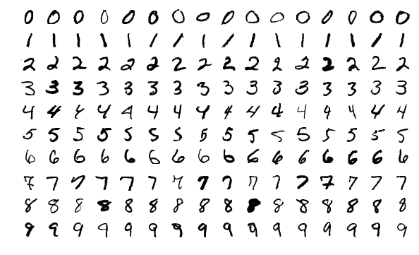
Figure 1. A small set of data samples from the MNIST database.

The MNIST dataset consists of 70000 images of handwritten digits, and the same number of labels denoting the value in each image. A label is a qualitative value that classifies the input image. In this paper, 50000 images will be used for training, and 10000 for validation. Each image is a 28 by 28 pixel greyscale scan of a numerical digit in the range [0-9]. The labels for this dataset are thus numerical values in the same range. Figure 2 offers a close-up view of one such image, labeled as number 2.

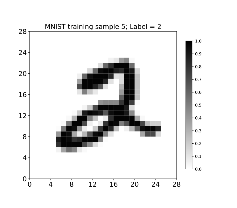
Figure 2. A close-up view at a single digit sample of 28 by 28 pixels. The value of each pixel is the greyscale intensity, zero for white and one for black.

In this example, we will load the MNIST dataset into memory, the data from each image being represented as a rank-1 real array of 784 elements, with magnitude in the range [0-1]. The pixel values from each image will serve as the input data $x$ to our network. The labels will serve as the output data $y$. Rather than a single number indicating the value of the label, we will use an array of 10 elements, one for each digit. The values of the elements will be zero for all elements except the one corresponding to the value of the label, which will take the value of one. Listing 12 shows the complete program.

⬇

program example_mnist

use mod_kinds, only: ik, rk

use mod_mnist, only: label_digits, load_mnist

use mod_network, only: network_type

implicit none

real(rk), allocatable :: tr_images(:,:), tr_labels(:)

real(rk), allocatable :: te_images(:,:), te_labels(:)

real(rk), allocatable :: input(:,:), output(:,:)

type(network_type) :: net

integer(ik) :: i, n, num_epochs

integer(ik) :: batch_size, batch_start, batch_end

real(rk) :: pos

call load_mnist(tr_images, tr_labels, te_images, te_labels)

net = network_type([784, 30, 10])

batch_size = 1000

num_epochs = 30

if (this_image() == 1) then

write(*, ’(a,f5.2,a)’) ’Initial accuracy: ’,&

net % accuracy(te_images, label_digits(te_labels)) * 100, ’ %’

end if

epochs: do n = 1, num_epochs

mini_batches: do i = 1, size(tr_labels) / batch_size

! pull a random mini-batch from the dataset

call random_number(pos)

batch_start = int(pos * (size(tr_labels) - batch_size + 1))

batch_end = batch_start + batch_size - 1

! prepare mini-batch

input = tr_images(:,batch_start:batch_end)

output = label_digits(tr_labels(batch_start:batch_end))

! train the network on the mini-batch

call net % train(input, output, eta=3._rk)

end do mini_batches

if (this_image() == 1) then

write(*, ’(a,i2,a,f5.2,a)’) ’Epoch ’, n, ’ done, Accuracy: ’,&

net % accuracy(te_images, label_digits(te_labels)) * 100, ’ %’

end if

end do epochs

end program example_mnist

Listing 12: The complete program to train and evaluate a neural network using the MNIST dataset of handwritten digits.

This program has 3 key pieces. First, it loads the training and testing data into the memory by calling the load_mnist subroutine. This subroutine returns input and output data arrays that are in the appropriate shape for working with neural-fortran. While not obvious from the listing, the training dataset consists of 50000 images, and the testing dataset consists of 10000 images. The distinction between the two is built into the data loader. It is important for the validation dataset to be completely distinct from the training dataset to ensure that the model can learn in a general way.

Second, we create our network instance, in this case a network with one input layer with 784 neurons, one hidden layer with 30 neurons, and one output layer with 10 neurons. Recall that the sizes of input and output layers are not arbitrary. The input layer size must match the size of the input data sample. In case of MNIST, each image is 28 by 28 pixels, a total of 784 pixels. Similarly, the size of the output layer must match the size of the output data sample, an array of 10 elements, one for each digit. The rationale for transforming the value of the image label into an array of 10 binary values is empirical. As the weights and biases of the network are adjusted in the training process, the network assigns higher probability to one or more digits. The output of the network is thus the probability that the input image represents each of the 10 digits. For a well trained network and a clean input image, the network should output one value that is approximately 1, and nine others that are approximately 0. This binary label representation thus allows for probabilistic output of the network. While other output layer configurations are possible, they don’t tend to yield as good results.

In the third step, we begin the training loop, which is performed for a set number of epochs. An epoch refers to one round of cycling through the whole training dataset, in our case, 50000 images. Within each epoch, however, we iterate over a number of so-called mini-batches, which are the subsets of the whole dataset. The number of mini-batches is controlled by the batch size, in our case 1000, meaning that a total of 50 training iterations will be done in each epoch. The random choice of the starting index of the mini-batch makes this gradient descent approach a stochastic one. Randomly sampling the training data in each batch prevents the network from converging toward a state that is specific to the ordering of the data. Note that in this simplistic implementation using the random_number subroutine, not all data samples will be used even for a large number of epochs, and there will be some overlap within each epoch. While this works well enough for this example, more sophisticated shuffling should be used in production.

As we saw in Section 3.3, the learning rate eta is the multiplier to weight and bias tendencies at the time of the network update. Its value is somewhat arbitrary and varies between applications. An optimal value of eta thus needs to be determined by experimentation whenever we work with new datasets or network structures. A value of eta that is too high may lead to never converging to a local minimum of the cost function. On the other hand, a value too low may lead to a slow and computationally expensive training procedure.

The neural-fortran API used in this example is rather simple. We used only a network constructor and two methods, accuracy(), and train(). All other code was for the purpose of loading and preparing the training data, slicing mini-batches out of the whole dataset, and other housekeeping.

Running this program outputs the following:

⬇

Initial accuracy: 10.09 %

Epoch 1 done, Accuracy: 27.91 %

Epoch 2 done, Accuracy: 53.17 %

Epoch 3 done, Accuracy: 75.16 %

Epoch 4 done, Accuracy: 82.96 %

Epoch 5 done, Accuracy: 87.24 %

...

Epoch 30 done, Accuracy: 93.39 %

Listing 13: Output from the MNIST training example program. Some lines omitted for brevity.

The program first outputs the initial accuracy, which is approximately 10%. The accuracy is calculated as the number of digits (out of 10000, the size of the testing dataset) that are correctly predicted by the network. Since we have not done any training at this point, the accuracy is equivalent to that of a random guess of one in ten digits. With each epoch, the accuracy steadily improves and exceeds 93% at the 30th epoch. While this is not an extraordinarily high accuracy for handwritten digit recognition, it demonstrates that our simple little network works as intended. For example, a deep 6-layer network with several thousand neurons was shown to achieve accuracy of 99.65% (Ciresan et al., 2010).

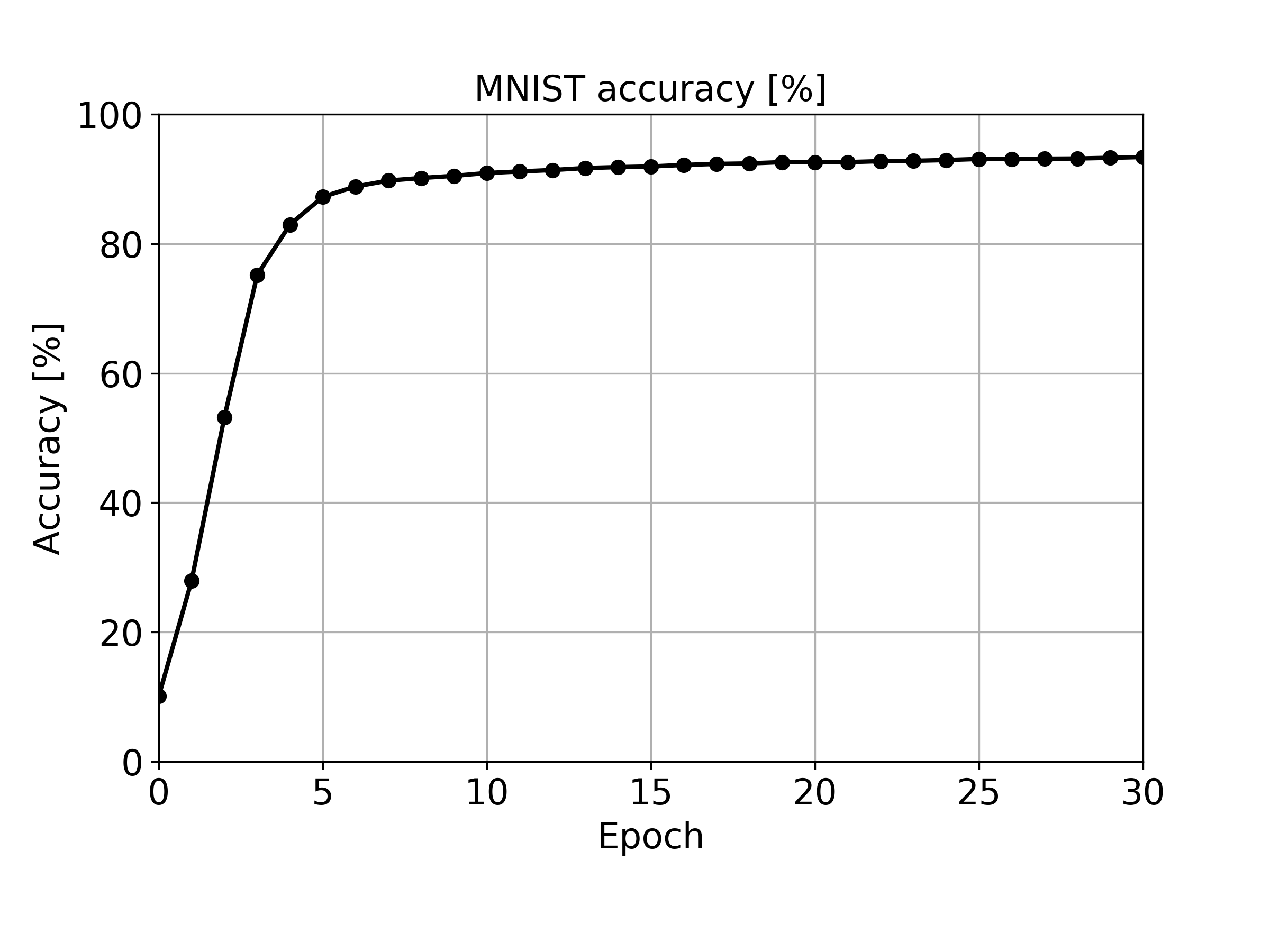
Figure 3. Accuracy as function of the number of epochs in the MNIST example.

The network accuracy as function of number of epochs is shown on Figure 3. It shows that the fastest learning occurs during the first five epochs, beyond which the network learns slowly and eventually plateaus. The rate of the increase in accuracy, and the final value at which the accuracy asymptotes is sensitive to almost every aspect of the network: Number of layers and neurons in each layer, batch size, learning rate, the choice of activation and cost functions, the initialization method for weights and biases, and more.

5. Computational performance

We evaluate two aspects of computational performance of neural-fortran: Serial performance in comparison with an established machine learning framework, and parallel scalability. Both benchmarks were done with the following configuration:

• Processor: Intel Xeon Platinum 8168 (2.70GHz)

• Operating System: Fedora 28 64-bit

• Compiler: GNU Fortran 8.2.1

• Libraries:

  • OpenMPI 2.1.1

  • OpenCoarrays 2.3.1 (Fanfarillo et al., 2014)

5.1. Serial performance

To evaluate the serial (single-core) performance of neural-fortran, we compare the elapsed training time of neural-fortran against an established and mature machine learning framework, Keras 2.2.4 (Chollet et al., 2015) using Tensorflow 1.12.0 (Abadi et al., 2016) as the computational backend. This framework was configured in a Python 3.6.8 environment with numpy 1.16.1 and scipy 1.2.1 on the same system used to run neural-fortran.

The performance is compared using the handwritten digits example with MNIST image dataset, with the same layer configuration as that used in Section 4 (784-30-10 neurons with sigmoid activations). The Keras network was configured in the exact same fashion, with stochastic gradient descent optimizer and the quadratic cost function. The default batch size for Keras is 32 if not specified, so we use that value in this comparison. A total of 10 training epochs are done in each run. As the Tensorflow backend engages multithreading by default, we explicitly limit the number of cores and threads to one, for fairness. A total of 5 runs are made, the mean and standard deviation of which are shown in Table 1.

Table 1. Computational performance of neural-fortran and Keras+Tensorflow in the MNIST training example. Elapsed time shown is the mean $\pm$ standard deviation of 5 repeated runs.

Framework	Elapsed (s)	Memory use (MB)
neural-fortran	13.933 $\pm$ 0.378	220
Keras + Tensorflow	12.419 $\pm$ 0.474	359

This basic comparison of serial performance between neural-fortran and Keras + Tensorflow in the MNIST training example demonstrates that they are similar to each other. The elapsed time is 12% longer in the case of neural-fortran on average, and 20% less variable between individual runs. This is likely because the neural-fortran program is more ”bare-bones”, in contrast to the Keras program that at a high level goes through the Python interpreter, which may add some unpredictable overhead. neural-fortran also uses about 39% less memory than Keras with Tensorflow, meaning that it could be used to solve larger problems within equivalent memory constraints. Although Keras + Tensorflow marginally outperforms neural-fortran in terms of average run-time, it’s important to note that neural-fortran’s core computations are not optimized, but expressed as a a concise proof of concept. Considering that Keras and Tensorflow are mature frameworks that are used widely in production and at scale, this suggests that neural-fortran has potential to be computationally competitive in production, especially if optimizations are made to the linear algebra operations.

Finally, it is worth comparing the ease of use of neural-fortran to that of Keras. The most straightforward metric is the number of lines of code needed to construct, train, and evaluate the network. The neural-fortran program used in this benchmark consists of 35 lines of code excluding comments, whereas the Keras script consists of 41 lines of code. Five of these lines were needed to constrain the Keras network to use a single thread. The amount of code needed for this example is thus almost equivalent between the two frameworks. The Python script used to construct, train, and time the Keras network, and the neural-fortran program used in this benchmark are available in the source code repository for this paper.

5.2. Parallel scaling

With a basic measure of serial performance established, let’s evaluate neural-fortran’s parallel scaling. All network parameters are the same as in the serial case, except for the batch size, which is now set to 1200. A large batch size is important for parallel scaling because a single batch is distributed evenly between the parallel processes. Unlike in the serial benchmarks, here we time only the traning portion of the code and exclude the loading of the dataset. Elapsed times on up to 12 parallel images on a shared-memory system are shown in Figure 4. The elapsed time decreases monotonically from over 12 s in serial mode to under 2 s on 12 parallel cores.

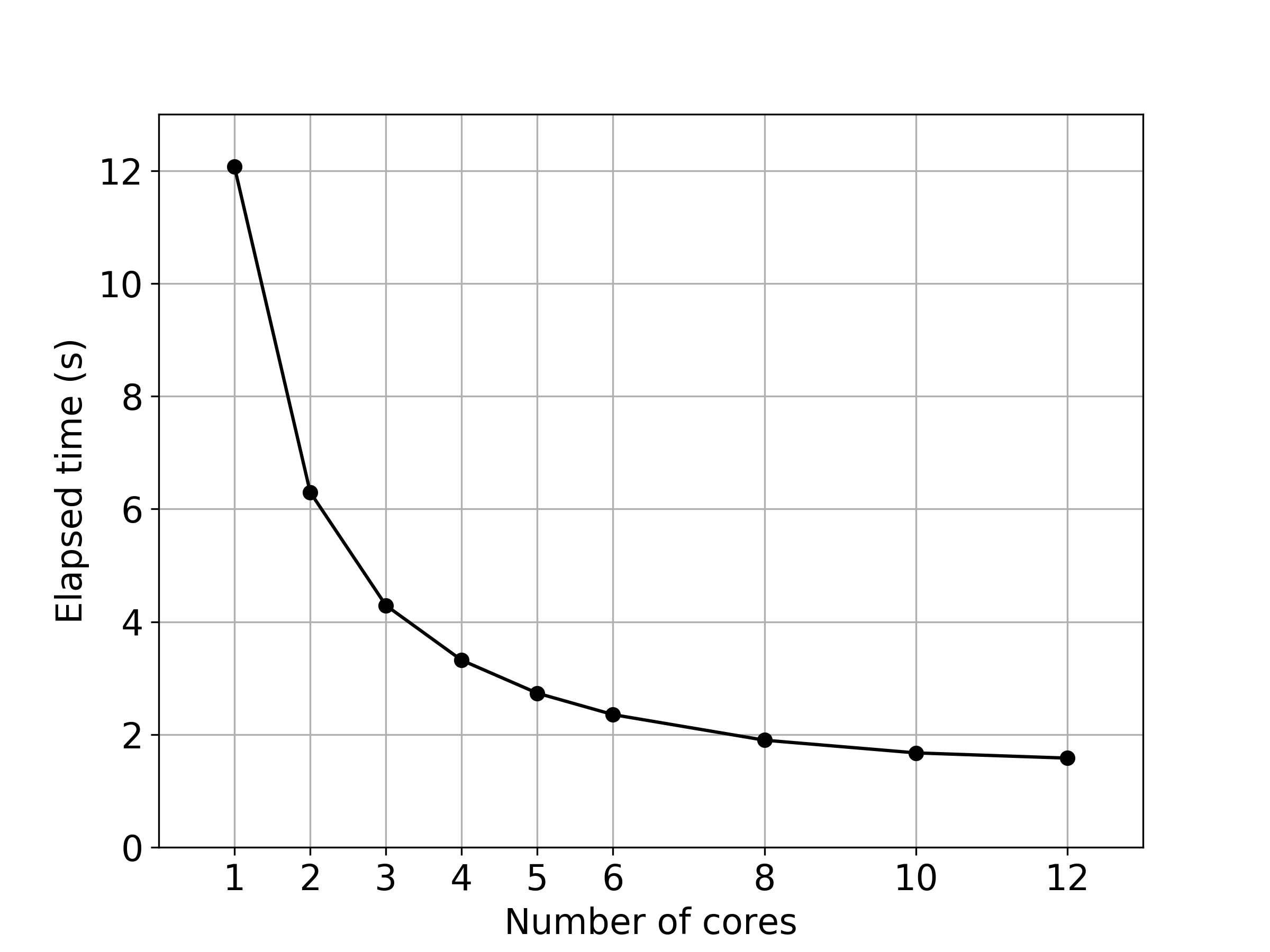
Figure 4. Mean elapsed time as function of number of cores in the MNIST training example.

Next we look at the parallel efficiency (PE), which is the serial elapsed time divided by the parallel elapsed time and the number of processes, $PE=t(1)/(nt(n))$ (Figure 5). On the high end, perfect scaling corresponds $PE=1$. On the low end, no parallel speed-up relative to the serial performance, meaning $t(n)=t(1)$ for any value of $n$, corresponds to $PE=1/n$ and is shown using the dashed line.

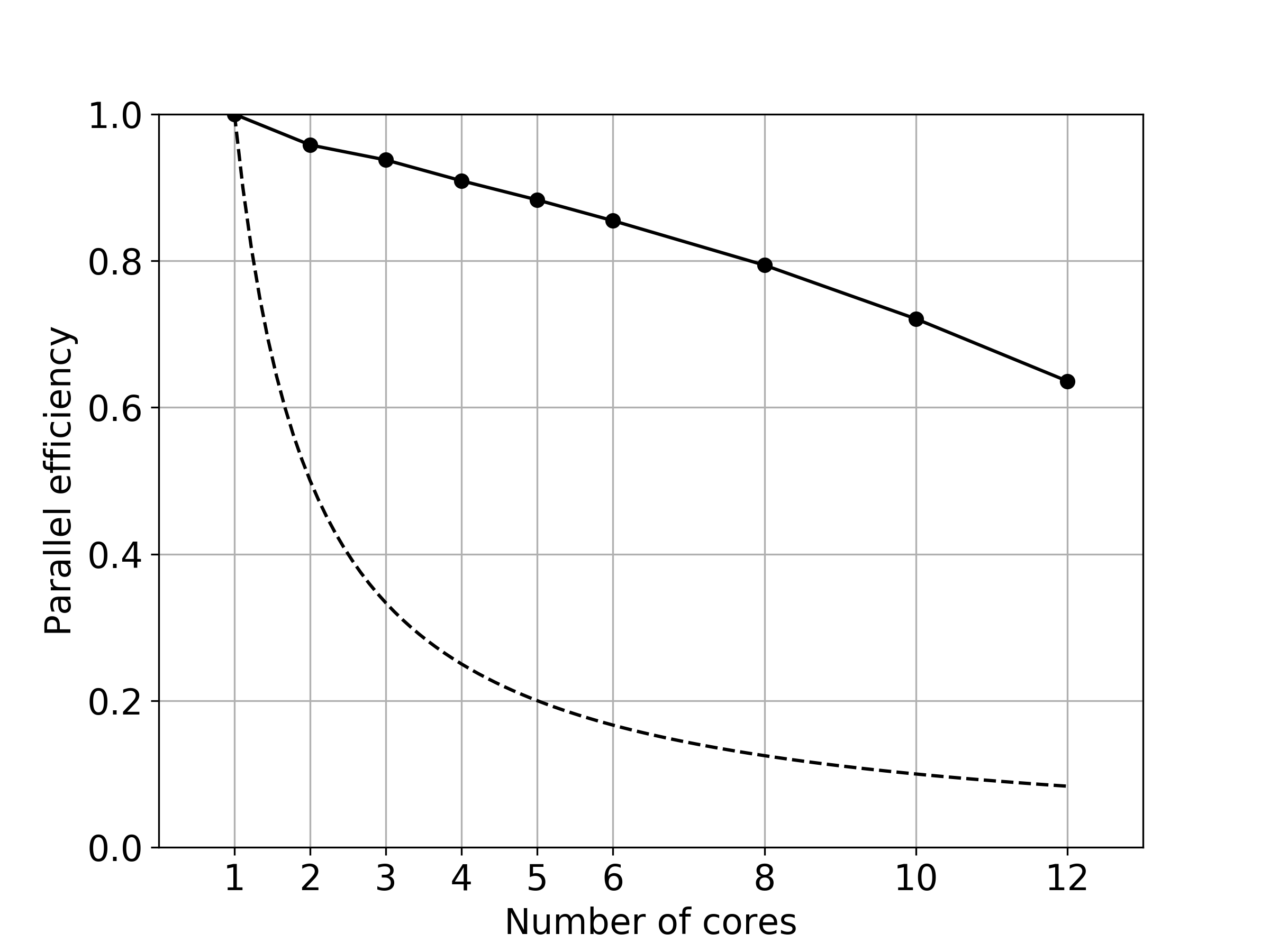
Figure 5. Parallel efficiency as function of number of cores in the MNIST training example (solid line), and zero speed-up relative to the serial mode, $PE=1/n$ (dashed line).

The mean elapsed times and their standard deviation (out of five runs) are given in Table 2.

Table 2. Parallel scaling of neural-fortran in the MNIST training example.

Cores	Elapsed (s)	Parallel efficiency
1	12.068 $\pm$ 0.136	1.000
2	6.298 $\pm$ 0.043	0.958
3	4.290 $\pm$ 0.026	0.938
4	3.318 $\pm$ 0.005	0.909
5	2.733 $\pm$ 0.005	0.883
6	2.353 $\pm$ 0.016	0.855
8	1.900 $\pm$ 0.019	0.794
10	1.674 $\pm$ 0.012	0.721
12	1.581 $\pm$ 0.046	0.636

Going from a single to 12 parallel cores, the parallel efficiency drops to 64%. With increasing number of parallel processes, the computational load decreases because the batch of the same size is divided into smaller pieces. Conversely, the amount of communication between processes that needs to be done by the collective sum of weight and bias tendencies increases. This is analogous to the scalability limits in fluid dynamics, except that here the parallel operation is global, rather than only between the neighboring processes. Nevertheless, the measured $PE$ remains well above the zero-speed-up line for all configurations, indicating that in this example neural-fortran can efficiently use all cores in a high-end shared memory system. The ability to explicitly allocate any number of cores in the system, or to execute the training on a distributed-memory system without any change to the code, are unique features of neural-fortran that are not trivial to accomplish in a framework like Keras or Tensorflow.

6. Conclusions

This paper described the implementation of neural-fortran, a parallel framework for neural networks and deep learning. It allows constructing feed-forward neural networks with any number of layers and neurons and offers several activation functions and learning via stochastic gradient descent. neural-fortran also leverages the collecive sum and broadcast procedures introduced in Fortran 2018 to accomplish data-based parallelism. Model-based parallelism can be enabled by linking to external linear algebra libraries such the Intel MKL or ATLAS. Use of neural-fortran was demonstrated in an example of training the network to recognize handwritten digits. In a rudimentary benchmark, computational performance of neural-fortran is comparable to an established and mature framework (Keras + Tensorflow), making it a viable candidate for use in production. While currently only a proof of concept with a limited number of features, neural-fortran provides a good foundation for further development and applications.

There are two potential benefits of using neural-fortran in new software development and machine learning projects. One is tight integration with existing Fortran code, such as computational fluid dynamics for engineering applications, or numerical weather prediction. For example, efforts to augment existing climate modeling capabilities are underway, one instance being the Earth Machine project (Schneider et al., 2017; Voosen, 2018). Such projects work with large Fortran code bases with many parametric and empirical sub-models that could be largely accelerated via tight integration with a machine learning framework such as neural-fortran. Another benefit is the ease of use for experienced Fortran programmers who want to get started with machine learning and neural networks without needing to also learn another programming language or framework. For this reason, any further development of neural-fortran will maintain ease of use as its primary focus.

- (1)
- Abadi et al. (2016) M. Abadi, P. Barham, J. Chen, Z. Chen, A. Davis, J. Dean, M. Devin, S. Ghemawat, G. Irving, M. Isard, et al. 2016. Tensorflow: a system for large-scale machine learning.. In OSDI, Vol. 16. 265–283.
- Chassignet et al. (2006) E. P. Chassignet, H. E. Hurlburt, O. M. Smedstad, G. R. Halliwell, P. J. Hogan, A. J. Wallcraft, and R. Bleck. 2006. Ocean prediction with the hybrid coordinate ocean model (HYCOM). In Ocean weather forecasting. Springer, 413–426.
- Chollet et al. (2015) F. Chollet et al. 2015. Keras. https://keras.io.
- Ciresan et al. (2010) D. C. Ciresan, U. Meier, L. M. Gambardella, and J. Schmidhuber. 2010. Deep, Big, Simple Neural Nets for Handwritten Digit Recognition. Neural Computation 22, 12 (2010), 3207–3220. https://doi.org/10.1162/NECO_a_00052
- Donelan et al. (2012) M. A. Donelan, M. Curcic, S. S. Chen, and A. K. Magnusson. 2012. Modeling waves and wind stress. Journal of Geophysical Research: Oceans 117, C11 (2012).
- Fanfarillo et al. (2014) A. Fanfarillo, T. Burnus, V. Cardellini, S. Filippone, D. Nagle, and D. Rouson. 2014. OpenCoarrays: open-source transport layers supporting coarray Fortran compilers. In Proceedings of the 8th International Conference on Partitioned Global Address Space Programming Models. ACM, 4.
- Fischer et al. (2008) P. F. Fischer, J. W. Lottes, and S. G. Kerkemeier. 2008. nek5000. http://nek5000.mcs.anl.gov
- Glorot and Bengio (2010) X. Glorot and Y. Bengio. 2010. Understanding the difficulty of training deep feedforward neural networks. In Proceedings of the thirteenth international conference on artificial intelligence and statistics. 249–256.
- Goldberg (2016) Y. Goldberg. 2016. A primer on neural network models for natural language processing. Journal of Artificial Intelligence Research 57 (2016), 345–420.
- Hochreiter and Schmidhuber (1997) S. Hochreiter and J. Schmidhuber. 1997. Long short-term memory. Neural computation 9, 8 (1997), 1735–1780.
- Hurrell et al. (2013) J. W. Hurrell, M. M. Holland, P. R. Gent, S. Ghan, Jennifer E. Kay, P. J. Kushner, J.-F. Lamarque, W. G. Large, D. Lawrence, K. Lindsay, W. H. Lipscomb, M. C. Long, N. Mahowald, D. R. Marsh, R. B. Neale, P. Rasch, S. Vavrus, M. Vertenstein, D. Bader, W. D. Collins, J. J. Hack, J. Kiehl, and S. Marshall. 2013. The Community Earth System Model: A Framework for Collaborative Research. Bulletin of the American Meteorological Society 94, 9 (2013), 1339–1360. https://doi.org/10.1175/BAMS-D-12-00121.1
- Kimoto et al. (1990) T. Kimoto, K. Asakawa, M. Yoda, and M. Takeoka. 1990. Stock market prediction system with modular neural networks. In 1990 IJCNN international joint conference on neural networks. IEEE, 1–6.
- Krizhevsky and Hinton (2009) A. Krizhevsky and G. Hinton. 2009. Learning multiple layers of features from tiny images. Technical Report. Citeseer.
- Krizhevsky et al. (2012) A. Krizhevsky, I. Sutskever, and G. E. Hinton. 2012. Imagenet classification with deep convolutional neural networks. In Advances in neural information processing systems. 1097–1105.
- Kutz (2017) J. Nathan Kutz. 2017. Deep learning in fluid dynamics. Journal of Fluid Mechanics 814 (2017), 1–4. https://doi.org/10.1017/jfm.2016.803
- LeCun et al. (1998) Y. LeCun, L. Bottou, Y. Bengio, and P. Haffner. 1998. Gradient-based learning applied to document recognition. Proc. IEEE 86, 11 (1998), 2278–2324.
- Paszke et al. (2017) A. Paszke, S. Gross, S. Chintala, G. Chanan, E. Yang, Z. DeVito, Z. Lin, A. Desmaison, L. Antiga, and A. Lerer. 2017. Automatic differentiation in PyTorch. In NIPS-W.
- Pedregosa et al. (2011) F. Pedregosa, G. Varoquaux, A. Gramfort, V. Michel, B. Thirion, O. Grisel, M. Blondel, P. Prettenhofer, R. Weiss, V. Dubourg, J. Vanderplas, A. Passos, D. Cournapeau, M. Brucher, M. Perrot, and E. Duchesnay. 2011. Scikit-learn: Machine Learning in Python. Journal of Machine Learning Research 12 (2011), 2825–2830.
- Powers et al. (2017) J. G. Powers, J. B. Klemp, W. C. Skamarock, C. A. Davis, J. Dudhia, D. O. Gill, J. L. Coen, D. J. Gochis, R. Ahmadov, S. E. Peckham, G. A. Grell, J. Michalakes, S. Trahan, S. G. Benjamin, C. R. Alexander, G. J. Dimego, W. Wang, C. S. Schwartz, G. S. Romine, Z. Liu, C. Snyder, F. Chen, M. J. Barlage, W. Yu, M. G., and Duda. 2017. The Weather Research and Forecasting Model: Overview, System Efforts, and Future Directions. Bulletin of the American Meteorological Society 98, 8 (2017), 1717–1737. https://doi.org/10.1175/BAMS-D-15-00308.1
- Reid (2018) John Reid. 2018. The new features of Fortran 2018. In ACM SIGPLAN Fortran Forum, Vol. 37. ACM, 5–43.
- Rumelhart et al. (1986) D. E. Rumelhart, G. E. Hinton, and R. J. Williams. 1986. Learning representations by back-propagating errors. Nature 323 (Oct. 1986), 533–536. https://doi.org/10.1038/323533a0
- Schneider et al. (2017) T. Schneider, S. Lan, A. Stuart, and J. Teixeira. 2017. Earth System Modeling 2.0: A Blueprint for Models That Learn From Observations and Targeted High-Resolution Simulations. Geophysical Research Letters 44, 24 (2017), 12,396–12,417. https://doi.org/10.1002/2017GL076101
- Valiev et al. (2010) M. Valiev, E. J. Bylaska, N. Govind, K. Kowalski, T. P. Straatsma, H. J. J. Van Dam, D. Wang, J. Nieplocha, E. Apra, T. L. Windus, and W. A. de Jong. 2010. NWChem: a comprehensive and scalable open-source solution for large scale molecular simulations. Computer Physics Communications 181, 9 (2010), 1477–1489.
- Voosen (2018) P. Voosen. 2018. The Earth Machine. Science 361, 6400 (2018), 344–347. https://doi.org/10.1126/science.361.6400.344
- Whaley and Petitet (2005) R. C. Whaley and A. Petitet. 2005. Minimizing development and maintenance costs in supporting persistently optimized BLAS. Software: Practice and Experience 35, 2 (2005), 101–121.
- Whaley et al. (2001) R. C. Whaley, A. Petitet, and J. J. Dongarra. 2001. Automated Empirical Optimization of Software and the ATLAS Project. Parallel Comput. 27, 1–2 (2001), 3–35.