A highly variable methanol maser in G111.256$-$0.770

Abstract

G111.256$-$0.770 is a high-mass young stellar object associated with a weak 6.7 GHz methanol maser showing strong variability. We present results of a multi-epoch monitoring program of the target, conducted with the Torun 32 m telescope for more than a decade. We found that the isotropic maser luminosity varied by a factor 16 on a timescale of 5$-$6 yr and individual features showed small amplitude short-lived ($\sim$0.2 yr) bursts superimposed on higher amplitude slow (>5 yr) variations. The maser integrated flux density appears to be correlated with the near-infrared flux observed with the (NEO)WISE, supporting radiative pumping of the maser line.

1 Introduction

Methanol masers are one of the earliest observable signatures of high-mass young stellar objects (HMYSOs), lasting $\sim 10^{4}$ yr (van der Walt, 2005) before or during the formation of ultra-compact HII regions (Walsh et al. 1998; Ellingsen 2006; Urquhart et al. 2013; de Villiers et al. 2015). It is thought that they predominantly arise in the circumstellar discs or outflows (e.g. Moscadelli et al. 2016; Sanna et al. 2017) and one of the strongest transition at 6.7 GHz probes the molecular gas of density $10^{4}-10^{8}$ cm^-3 and temperature below 150 K (Cragg, Sobolev & Godfrey, 2005).

Recent studies have revealed the maser lines as sensitive indicators of sudden changes in the pumping conditions in the environments of two HMYSOs likely triggered by accretion bursts (Caratti o Garatti et al., 2017; Moscadelli et al., 2017; Hunter et al., 2018). Changes in the stellar luminosity due to accretion episodes appear to affect all maser features and the overall maser structure at 6.7 GHz in the HMYSO S255IR-IRS3 (Moscadelli et al., 2017) while turbulence in the molecular clouds may produce short-lived (a week to a few months) random flares not correlated across different features (Goedhart, Gaylard & van der Walt, 2004). When the maser beaming effect in an assembly of clouds of arbitrary geometry is considered then quasi-periodic variations of the maser intensity may result from the rotation of maser clouds across the line of sight (Gray, Mason & Etoka, 2018). Long-lived (several months to a few years) bursts may be caused by outflows or shock waves passing through the masing region (Goedhart et al. 2004; Dodson, Ojha & Ellingsen 2004). In the paper we report the results a long term monitoring of G111.256$-$0.770 (hereafter G111) at 6.7 GHz methanol transition which can shed more light on the processes affecting the masers.

The target is one of the most variable 6.7 GHz masers in the sample studied by Szymczak et al. (2018); the relative amplitude of individual features was up to 5.5 on timescales of between two months and a few years. The maser emission of isotropic luminosity $8.5\times 10^{-8}L_{\odot}$ (Wu et al., 2010) spatially coincides with the 22 GHz H₂O masers and the radio continuum source of spectral index 0.64 between 1.3 and 3.6 cm wavelength is consistent with free-free emission from a thermal jet or with a partially thick HII region (Trinidad et al., 2006). Observations of outflow tracers revealed both redshifted and blueshifted components that largely overlap on a scale lower than 10$-$15″  suggesting an outflow almost completely along the line of sight (Wu et al., 2010; Sánchez-Monge et al., 2013) while the H₂ line emission knots and the radio continuum elongation delineate a collimated jet of size 5$-$7″  at a position angle $-$44° (Massi et al., 2018). Most of the water maser components are blueshifted with respect to the systemic velocity of $-$44.5  km s^-1  (Sánchez-Monge et al. 2013) and come from a region of size up to 800$-$1000 au (Goddi et al., 2005; Moscadelli et al., 2016) for a trigonometric distance of 3.34 kpc (Choi et al. 2014). Their proper motions have orientations both parallel and transverse to the direction of the jet (Moscadelli et al., 2016) suggesting a low angle between the jet/outflow and the line of sight.

The present paper provides evidence that the 6.7 GHz methanol maser from G111 is significantly variable on a decade timescale.

2 Observations

For the analysis presented in the paper we used published (Szymczak et al. 2018) and unpublished archival 6.7 GHz maser data and new observations, all of which were obtained with the Torun 32 m radio telescope. The new observations were carried out from February 2013 to October 2018. The beam full width at half maximum of the antenna at 6.7 GHz was 5.8 arcmin and rms pointing error was $\sim$25 arcsec but it was reduced to 10 arcsec from mid-2016 (Lew 2018). The system temperature was between 25 and 40 K. The data were dual polarization taken in frequency switching mode using a 1 MHz shift. We used an autocorrelation spectrometer to acquire spectra with a resolution of 0.09  km s^-1and the typical rms noise level of 0.35 Jy before 2015 May and 0.25 Jy afterwards. The system was calibrated continuously against a noise diode of known constant temperature and this calibration was daily checked by observing the non-variable maser source G32.744$-$0.076 and regular observations of the continuum source 3C123 (Szymczak et al. 2018). The resulting accuracy of the absolute flux density was better than 10 per cent.

To quantify the observed variability we used variability coefficients. A Gaussian function profile fitting has also been performed. We estimated time scales with the structure function analysis and minimum-maximum method. A more detailed description of the methods used is presented in Appendix A.

3 Results

Figure 1: Top: 6.7 GHz maser spectra of G111. The average (solid), high (dashed) and low (dotted) emission levels are shown. Bottom: Plots of variability index (VI), fluctuation index (FI) and reduced $\chi^{2}$.

The average spectrum for the time-span from MJD 54583 to 58418 (685 observations) together with the spectra at high- and low-emission levels and plots of three variability measures are shown in Figure 1. The variability index ($VI$) and fluctuation index ($FI$) quantify the flux amplitude change in variable sources (Aller, Aller & Hughes, 2003) and are described in Appendix A. All four persistent features displayed high variability over the whole observing period (Table 1).

There are significant differences between $VI$ and $FI$ profiles which result from their properties; $FI$ is sensitive to changes in the flux density with low signal-to-noise ratio and its value is highest in the wings of the features, whereas $VI$ better depicts high amplitude variations.

The light curve of the velocity-integrated flux density is presented in Figure 2 where the new and archival observations are complemented with the discovery detection (Szymczak et al. 2000) and a single VLA observation (Hu et al. 2016). The emission peaked around MJD 55296 and 56340 and the second outburst has a FHWM of $\sim$256 d and the rising phase a factor of two shorter than the declining phase. In periods of low activity the emission linearly decreased with a rate of $-$0.17$\pm$0.02 Jy km s^-1yr^-1. The total flux density ranged from 0.9 to 14.5 Jy km s^-1 and the average value was 4.4$\pm$0.1 Jy km s^-1. For the adopted distance of 3.34 kpc the isotropic maser luminosity reached a peak of 1.0$\pm$0.2$\times 10^{-6}L_{\odot}$ around MJD 56340 and declined to 8.9$\pm$1.9$\times 10^{-8}L_{\odot}$ at the end of the monitoring period. The median luminosity equals to 2.8$\times 10^{-7}L_{\odot}$ is a factor of 3.2 lower than that reported for the sample observed in a high sensitivity, untargeted survey with the Arecibo telescope (Pandian et al. 2009). This confirms that the source belongs to a population of weak methanol sources (Wu et al. 2010).

Table 1: Variability measures of the 6.7 GHz features. Variability index ($VI$), fluctuation index ($FI$) and $\chi^{2}_{\mathrm{r}}$ are for the mean velocity of feature while the average values $<VI>$, $<FI>$ and $<\chi^{2}_{\mathrm{r}}>$ and their standard errors are calculated for the given velocity range ($\Delta V$).

$V$	$VI$	$FI$	$\chi^{2}_{\mathrm{r}}$	$\Delta V$	$<VI>$	$<FI>$	$<\chi^{2}_{\mathrm{r}}>$
(km s-1)				(km s-1)
$-$41.22	0.79	0.38	9.68	$-$41.57;$-$40.65	0.68(0.18)	0.32(0.10)	5.44(3.15)
$-$38.85	0.93	0.34	24.25	$-$39.68;$-$38.19	0.88(0.07)	0.74(0.29)	20.39(14.31)
$-$37.84	0.92	0.59	17.78	$-$38.15;$-$37.40	0.85(0.14)	0.79(0.15)	11.67(6.31)
$-$36.83	0.93	0.36	10.97	$-$37.18;$-$36.44	0.77(0.16)	0.53(0.24)	8.52(6.08)

Figure 2: Time series for the velocity-integrated flux density of the 6.7 GHz methanol maser line. The black squares and magenta circles denote the archival Torun 32 m data and from Szymczak et al. (2018), respectively. The blue triangle refers to the first detection (Szymczak et al. 2000) and the black star marks the VLA observation at MJD 55990 (Hu et al. 2016).

The dynamic spectrum in Figure 3 visualizes the bulk variability and the bursting variability of 6.7 GHz maser emission. It was created using linear interpolation between consecutive 32 m dish spectra and the emission above $3\sigma$ level is shown. There are four spectral features in the spectrum and all of them display complex and high variability (Table 1).

Figure 3: False-colour image of the 6.7 GHz maser flux density versus velocity and time. Velocities are measured in the frame of the local standard of rest. Individual observation dates are indicated by the vertical bars below the top horizontal axis. The two longest intervals with no data are blanked.

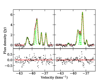
Figure 4: Examples of Gaussian profile fits to the spectra taken at MJD 55203 (left) and MJD 56276 (right).

3.1 Specific variability

In the following we deal with specific aspects of variability of the source.

The Gaussian analysis of profiles revealed a strong blending effect in some velocity ranges at different epochs (Fig. 4). For instance the emission of middle velocity features from $-$39.6 to $-$38.3 km s^-1  is composed of two Gaussian components at two time intervals of MJD 54680$-$56024 and MJD 56177$-$56485 (Figs. 3 and 5). In the first and second time-spans the emission peaked at $-$39.15 and $-$38.85 km s^-1  and at $-$38.79 and $-$38.41 km s^-1 , respectively. Changes in the flux density and line width of the bursting features near $-$39.15 and $-$38.41 km s^-1  generally followed that for the persistent emission with a mean velocity of $-$38.8 km s^-1. From MJD 55418 to 57011 this persistent emission showed a drift in velocity of 0.071 km s^-1 yr^-1.

Figure 5: Peak velocity, line width at half maximum (FWHM) and peak flux density for Gaussian components of the emission near $-$38.7 km s^-1. The red circles and green squares denote maser components appeared at slightly different velocities.

Figure 6 illustrates the behaviour of the emission near $-$36.7 km s^-1. The feature showed a long lasting ($\sim$700 d) burst with a peak of $\sim$5 Jy around MJD 55295 and several short ($<$200 d) less visible bursts and it dropped below our sensitivity level at the end of monitoring. No significant variations in the FWHM were seen. A velocity drift of $-$0.019 km s^-1 yr^-1 occurred before MJD 57039 and changed to $-$0.043 km s^-1 yr^-1 afterwards.

Figure 6: Same as in Fig. 5 but for the emission near $-$36.8 km s^-1. The green horizontal lines refer to the mean value of FWHM, the dashed violet line denotes the detection level of 0.8 Jy. The blue (dashed) and red (dotted) lines mark 1$\sigma$ and 3$\sigma$ levels, respectively.

Figure 7 depicts the variability of two features during the bursts. For the feature $-$38.73 km s^-1  the rising phase of a burst is clearly seen; the flux density increased from $\sim$1.2 to $\sim$3.6 Jy over $\sim$306 d, the peak velocity remained stable but the FWHM decreased from 0.50 to 0.24 km s^-1. This may be attributed to unsaturated amplification despite the fact that the canonical relationship between the intensity and linewidth (Goldreich & Kwan, 1974) is not fulfilled. On the other hand the declining phase is poorly seen and there is no evidence for profile broadening after the maximum.

The emission near $-$37.88 km s^-1 showed a short (49 d) burst with rising and declining phases of 11 and 38 d, respectively. It is striking that the line width was nearly constant while the peak velocity drifted by 0.086 km s^-1  during a $\sim$31 d long burst. This phenomenon can appear when a factor triggering the burst propagates to nearby layers of similar gas temperature but slightly different radial velocity. As the maser features are redshifted relative to the systemic velocity the drift may trace inflow motion.

We conclude, the variability of 6.7 GHz maser in the source is characterised by short duration (2–5 months) bursts at slightly different velocities superimposed on long lasting (1.5$-$3 yr) high relative amplitude (4$-$16) changes in the flux density showing velocity drifts (up to $\sim$0.1 km s^-1 yr^-1) for some features.

Figure 7: Same as in Fig. 5 but for two exemplary bursts. Left and right panels refer to $-$38.73 and $-$37.88 km s^-1  features, respectively. The green vertical lines denote the start time of bursts and the red vertical marks the end of burst. The grey symbols represent the measurements with the flux density below 3$\sigma$ level.

3.2 Variability timescales and delays

In order to determine a variability timescale we used the discrete structure function and minimum-maximum method (see Appendix A, Fuhrmann et al. 2008). The structure functions for the four persistent features are presented in Figure 8 and values of variability timescales obtained with both methods are given in Table 2. The timescales for the features $-$41.22 and $-$36.83 km s^-1  are 1.5 to 1.7 yr. The uncertainties of these estimates are usually lower than 26 per cent with the exception of the $-$36.83 km s^-1  feature that shows only a monotonic decrease and $t_{\mathrm{sf}}$ could not be accurately determined.

Figure 8: Structure functions of the persistent maser features.

Table 2: Variability timescales for the spectral features. $t_{\mathrm{var}}$ and $t_{\mathrm{sf}}$ are the timescales calculated with the minimum-maximum method and the structure function, respectively.

Feature ( km s-1)	$t_{\mathrm{var}}$ (d)	$t_{\mathrm{sf}}$ (d)
$-$41.22	506.1 $\pm$ 130.9	605.5${}^{+60.1}_{-69.9}$
$-$38.85	107.7 $\pm$ 10.7	274.9${}^{+58.1}_{-82.5}$
$-$37.84	45.8 $\pm$ 5.1	533.3${}^{+90.7}_{-118.2}$
$-$36.83	608.1 $\pm$ 104.9	663.6${}^{+198.2}_{-323.7}$

The values of the variability timescales for features at $-$38.85 and $-$37.84 km s^-1  obtained by the two methods differ significantly (Table 2). This is probably due to the fact that $t_{\mathrm{var}}$ strongly relies on the individual choice of the minimum and maximum measurements that make it irrelevant for describing the long lasting burst variability. We conclude that the variability timescales of the methanol masers in G111 range from 0.7 to 1.8 yr.

In order to search for time lags we computed the discrete cross-correlation function (DCF, Edelson & Krolik 1988) between the three spectral features. The maximum value was obtained with the centroid $\tau_{\mathrm{c}}$ of the DCF given by $\tau_{\mathrm{c}}={\sum_{\mathrm{i}}\tau_{\mathrm{i}}\mathrm{DCF}_{\mathrm{i}}}/{\sum_{\mathrm{i}}\mathrm{DCF_{i}}}$. Following the method presented in detail by Peterson et al. (1998) and Fuhrmann et al. (2008) we performed Monte Carlo simulations to statistically estimate meaningful time lags and their uncertainties. The influence of uneven sampling and the measurement errors were taken into account by using random subsets of the two spectral features time series and by adding random Gaussian fluctuations constrained by the measurement errors. For two pairs of the spectral features ($-$38.85 km s^-1 vs $-$37.84 km s^-1 and $-$38.85 kms^-1 vs $-$36.83 km s^-1) the centroid of the DCF maximum was computed 1000 times. The DCF and cross-correlation peak distribution (CCPD) for one pair of features are shown in Figure 9. Table 3 summarizes the results for two pairs of features. The time delay of the peaks estimated between the two maser features ($-$38.85 and $-$37.83 km s^-1) in the timespan from $\sim$MJD 56200 to 56900 is 5 months. The delay of the peak of the redshifted emission ($-$36.83 km s^-1) has a too large uncertainty to be considered as reliable. A visual inspection of the light curves (Fig. 3) implies that the burst of feature $-$37.84 km s^-1  around MJD 56200 was advanced by 147 d relative to the burst of feature at $-$38.85 km s^-1. This crude estimation is in good agreement (within 20 per cent) with that presented in Table 3.

Figure 9: Left. Example of discrete correlation function between the light curves of features $-$38.85 and $-$37.84 km s^-1. Right. Cross-correlation peak distribution for the peak of the DCF.

Table 3: Time lags corresponding to the average centroids of the DCF peaks obtained from cross-correlation peak distributions. Uncertainty values correspond to 1$\sigma$ obtained from CCPDs.

Features ( km s-1)	$\tau$ (d)
$-$38.85 v.s. $-$37.84	$-$153.7 $\pm$ 6.8
$-$38.85 v.s. $-$36.83	210.4 $\pm$ 80.3

4 Discussion

Figure 10: (a) Part of the maser light curve from Fig. 2 with the IR relative fluxes superimposed. The maser relative velocity-integrated flux density and its 5 point averaged values are marked by grey circles and grey line, respectively. IR data are from WISE and NEOWISE observations at bands W1 ($3.4\mu$m, blue crosses) and W2 ($4.6\mu$m, red crosses). The corresponding relative average IR fluxes are denoted by blue circles and red squares, respectively. (b) Relationships between the maser and IR relative fluxes. The solid lines denote the linear least-square fits to the data.

Our monitoring revealed that the methanol emission from G111 has experienced complex and erratic variations for the last decade. In the following we discuss the observed characteristics which may shed light on the processes causing variability.

One of the important factors producing the maser variability can be changes in the pump rate. Since the 6.7 GHz transition is thought to be pumped by infrared photons (Sobolev et al., 1997; Cragg et al., 2005) we examine if the maser emission is related to the near infrared radiation. Data from the WISE and NEOWISE archives (Wright et al., 2010; Mainzer et al., 2011) were retrieved for the target to construct the light curves at 3.4 and 4.6$\mu$m. In Figure 10a we show an overlay of the relative IR light curves with the methanol maser light curve. The WISE and NEOWISE photometric observations were available for 11 sessions of length of 1 to 8 d (median 1.8 d) over time-span 2010$-$2017 exactly covering our monitoring period. The changes in the IR fluxes generally followed those observed in the 6.7 GHz integrated (over the whole spectrum) maser flux in the declining phase of the long lasting ($>$5 yr) burst. Monthly averages of the integrated flux density were compared with the mean IR flux at 11 epochs and Figure 10b shows a significant correlation between the relative IR and maser fluxes. Although the IR data are not available during the maser burst around MJD 56400 and the trend in the IR relative brightness over the time-span $\sim$MJD 55200$-$55570 does not follow a decrease in maser intensity, this relationship may support a scenario in which the 6.7 GHz maser is radiatively pumped and changes in the pump rate may cause the 6.7 GHz maser variability as it was firmly demonstrated for maser sources experiencing giant bursts (Caratti o Garatti et al., 2017; Hunter et al., 2018). IR observations of sufficient cadence are required to confirm this relationship for other variable sources.

We detected variations in the centroid velocity of the two maser features. The velocity drift of feature $-$38.7 km s^-1  before $\sim$MJD 57000 can be easily recognized as due to blending effect of two features showing temporal intensity variations because velocity jumps were clearly seen over certain timespans (Fig. 5). A similar effect may occur for the $-$36.8 km s^-1  feature with FWHM ranging from 0.30 to 0.45 km s^-1  over the monitoring period (Fig. 6) and the slope of the drift changed to steeper after $\sim$MJD 57000. In this case we cannot resolve blending components probably due to the low signal-to-noise ratio. The opposite sense of the velocity drifts reinforces the interpretation that the velocity of emission fluctuates rather than drifting steadily. One can conclude that the velocity drifts are caused by slow (<10 yr) variations in the flux density of a few features at very close velocities.

In G111 we sometimes observed correlated variations across two different features combined with short-lived (2$-$3 months) flares restricted to one feature (Figs. 3, 7). If this variability timescale is on the order of the shock crossing time, which determines the lifetime of velocity coherence along the line-of-sight necessary for the maser amplification then for a typical size of the methanol maser cloud of 4 au (Bartkiewicz et al., 2016) the shock velocity is larger than 70 km s^-1. It very unlikely that the methanol maser would survive such a shock. Random bursts indicate rather local changes in the maser conditions modified for instance by turbulence (Sobolev et al., 1998); a dispersion of turbulence velocity of about 1 km s^-1  could account for the observed short-lived bursts caused by changes in the velocity coherence.

5 Summary

We report new 6.7 GHz methanol maser observations of G111 obtained since 2013 which extend the previously published light curve to $\sim$11 yr. The maser emission is characterised by short duration (2-3 months) bursts superimposed on long lasting ($>$5 yr) variations with a relative amplitude of 4 to 16. The comparison of the maser integrated flux density with the near infrared emission may support the radiative pumping scheme of the maser line but infrared observations of sufficient cadence are required to draw a firm conclusion.

Appendix A Analysis methods

A.1 Statistical variability measures

We used the variability index as proposed by Aller et al. (2003)

$$VI=\frac{(S_{\mathrm{max}}-\sigma_{\mathrm{Smax}})-(S_{\mathrm{min}}-\sigma_{\mathrm{Smin}})}{(S_{\mathrm{max}}-\sigma_{\mathrm{Smax}})+(S_{\mathrm{min}}-\sigma_{\mathrm{Smin}})},$$ (1)

where $S_{\mathrm{max}}$ and $S_{\mathrm{min}}$ refer to the maximum and minimum flux densities, respectively, while $\sigma_{\mathrm{Smax}}$ and $\sigma_{\mathrm{Smin}}$ are the corresponding uncertainties of $S_{\mathrm{max}}$ and $S_{\mathrm{min}}$. This index is useful to estimate the amplitude of the variability accounting for the measurement uncertainties and is well determined when variability is much greater than measurement errors.

The second variability measure used is the fluctuation index (Aller et al., 2003)

$$FI=\left[\left(\frac{\sum S^{2}_{\mathrm{i}}w_{\mathrm{i}}-\overline{S}\sum S_{\mathrm{i}}w_{\mathrm{i}}}{N-1}-1\right)\frac{N}{\sum w_{\mathrm{i}}}\right]^{0.5}\frac{1}{\overline{S}},$$ (2)

where $N$ is the number of observations of the flux density $S_{\mathrm{i}}$ measured with error $\sigma_{\mathrm{i}}$, weight is $w_{\mathrm{i}}=\sigma_{i}^{-2}$ and $\overline{S}$ is the average flux density. This index well estimates variability of features with low signal-to-noise ratio.

We also examined variability by computing the reduced value of $\chi^{2}$.

$$\chi^{2}_{\mathrm{r}}=\frac{1}{N-1}\sum^{N}_{i=1}\left(\frac{S_{\mathrm{i}}-\overline{S}}{\sigma_{\mathrm{i}}}\right)^{2}$$ (3)

A.2 Time scales of variability

We calculated the discrete structure function

$$SF(\tau_{\mathrm{j}})=\sum_{i=1}^{n}[S(t_{\mathrm{i}})-S(t_{\mathrm{i}}+\tau_{\mathrm{j}})]^{2}$$ (4)

for each data set $S(t_{\mathrm{i}})$ following the procedure described in Heeschen et al. (1987). Here, $n$ is the number of flux density measurements obtained at epochs $t_{\mathrm{i}}$ and $t_{\mathrm{i}}+\tau_{\mathrm{j}}$. We binned the data in 31 d intervals to get evenly sampled dataset. Two linear fits were performed to estimate the slope ($a\tau^{\beta}$) of the $SF$ before the first maximum and the mean value of $SF$ after the first maximum which estimates the saturation level $\rho_{0}$. The timescale of variability was then determined from formula

$$t_{\mathrm{sf}}=\left(\frac{\rho_{0}}{a}\right)^{\frac{1}{\beta}}$$ (5)

References

- Aller et al. (2003) Aller M. F., Aller H. D., Hughes P. A., 2003, ApJ, 586, 33
- Bartkiewicz et al. (2016) Bartkiewicz A., Szymczak M., van Langevelde H. J., 2016, A&A, 587, A104
- Caratti o Garatti et al. (2017) Caratti o Garatti A., et al., 2017, Nature Physics, 13, 276
- Choi et al. (2014) Choi Y. K., Hachisuka K., Reid M. J., Xu Y., Brunthaler A., Menten K. M., Dame T. M., 2014, ApJ, 790, 99
- Cragg et al. (2005) Cragg D. M., Sobolev A. M., Godfrey P. D., 2005, MNRAS, 360, 533
- Dodson et al. (2004) Dodson R., Ojha R., Ellingsen S. P., 2004, MNRAS, 351, 779
- Edelson & Krolik (1988) Edelson R. A., Krolik J. H., 1988, ApJ, 333, 646
- Ellingsen (2006) Ellingsen S. P., 2006, ApJ, 638, 241
- Fuhrmann et al. (2008) Fuhrmann L., et al., 2008, A&A, 490, 1019
- Goddi et al. (2005) Goddi C., Moscadelli L., Alef W., Tarchi A., Brand J., Pani M., 2005, A&A, 432, 161
- Goedhart et al. (2004) Goedhart S., Gaylard M. J., van der Walt D. J., 2004, MNRAS, 355, 553
- Goldreich & Kwan (1974) Goldreich P., Kwan J., 1974, ApJ, 190, 27
- Gray et al. (2018) Gray M. D., Mason L., Etoka S., 2018, MNRAS, 477, 2628
- Heeschen et al. (1987) Heeschen D. S., Krichbaum T., Schalinski C. J., Witzel A., 1987, AJ, 94, 1493
- Hu et al. (2016) Hu B., Menten K. M., Wu Y., Bartkiewicz A., Rygl K., Reid M. J., Urquhart J. S., Zheng X., 2016, ApJ, 833, 18
- Hunter et al. (2018) Hunter T. R., et al., 2018, ApJ, 854, 170
- Lew (2018) Lew B., 2018, Experimental Astronomy, 45, 81
- Mainzer et al. (2011) Mainzer A., et al., 2011, ApJ, 731, 53
- Massi et al. (2018) Massi F., Moscadelli L., Arcidiacono C., Bacciotti F., 2018, in Tarchi A., Reid M. J., Castangia P., eds, IAU Symposium Vol. 336, Astrophysical Masers: Unlocking the Mysteries of the Universe. pp 289–290, doi:10.1017/S1743921317011644
- Moscadelli et al. (2016) Moscadelli L., et al., 2016, A&A, 585, A71
- Moscadelli et al. (2017) Moscadelli L., et al., 2017, A&A, 600, L8
- Pandian et al. (2009) Pandian J. D., Menten K. M., Goldsmith P. F., 2009, ApJ, 706, 1609
- Peterson et al. (1998) Peterson B. M., Wanders I., Horne K., Collier S., Alexander T., Kaspi S., Maoz D., 1998, PASP, 110, 660
- Sánchez-Monge et al. (2013) Sánchez-Monge Á., López-Sepulcre A., Cesaroni R., Walmsley C. M., Codella C., Beltrán M. T., Pestalozzi M., Molinari S., 2013, A&A, 557, A94
- Sanna et al. (2017) Sanna A., Moscadelli L., Surcis G., van Langevelde H. J., Torstensson K. J. E., Sobolev A. M., 2017, A&A, 603, A94
- Sobolev et al. (1997) Sobolev A. M., Cragg D. M., Godfrey P. D., 1997, A&A, 324, 211
- Sobolev et al. (1998) Sobolev A. M., Wallin B. K., Watson W. D., 1998, ApJ, 498, 763
- Szymczak et al. (2000) Szymczak M., Hrynek G., Kus A. J., 2000, A&AS, 143, 269
- Szymczak et al. (2018) Szymczak M., Olech M., Sarniak R., Wolak P., Bartkiewicz A., 2018, MNRAS, 474, 219
- Trinidad et al. (2006) Trinidad M. A., Curiel S., Torrelles J. M., Rodríguez L. F., Migenes V., Patel N., 2006, AJ, 132, 1918
- Urquhart et al. (2013) Urquhart J. S., et al., 2013, MNRAS, 431, 1752
- Walsh et al. (1998) Walsh A. J., Burton M. G., Hyland A. R., Robinson G., 1998, MNRAS, 301, 640
- Wright et al. (2010) Wright E. L., et al., 2010, AJ, 140, 1868
- Wu et al. (2010) Wu Y. W., Xu Y., Pandian J. D., Yang J., Henkel C., Menten K. M., Zhang S. B., 2010, ApJ, 720, 392
- de Villiers et al. (2015) de Villiers H. M., et al., 2015, MNRAS, 449, 119
- van der Walt (2005) van der Walt J., 2005, MNRAS, 360, 153