Low-energy lepton physics in the MRSSM:
$(g-2)_{\mu}$, $\mu\to e\gamma$ and $\mu\to e$ conversion

Abstract

Low-energy lepton observables are discussed in the Minimal R-symmetric Supersymmetric Standard Model. We present comprehensive numerical analyses and the analytic one-loop results for $(g-2)_{\mu}$, $\mu\to e\gamma$, and $\mu\to e$ conversion. The interplay between the three observables is investigated as well as the parameter regions with large $g-2$. A striking difference to the MSSM is the absence of $\tan\beta$ enhancements; however we find smaller enhancements governed by MRSSM-specific R-Higgsino couplings $\lambda_{d}$ and $\Lambda_{d}$. As a result we find significant contributions to $g-2$ only in a small parameter space with several SUSY masses below $200$ GeV, compressed spectra and large $\lambda_{d}$, $\Lambda_{d}$. In this parameter space there is a correlation between all three considered observables. In the parameter region with small $(g-2)_{\mu}$ the SUSY masses can be larger and the correlation between $\mu\to e\gamma$ and $\mu\to e$ conversion is weak. Therefore already COMET Phase 1 has a promising sensitivity to the MRSSM.

1 Introduction

Low-energy lepton physics is an area which could lead to fundamental discoveries in the forthcoming years, and intriguing anomalies and deviations from Standard Model (SM) predictions have accumulated in observables related to leptons. In particular, there currently is a $3$–$4\sigma$ discrepancy in the muon anomalous magnetic moment $a_{\mu}$. Future measurements of $a_{\mu}$ are ongoing at Fermilab Grange:2015fou and planned at J-PARC Iinuma:2011zz ; Mibe:2011zz , with the prospect of a significant reduction of the uncertainty and the potential to firmly establish the existence of physics beyond the SM.

In addition, several measurements of charged lepton flavour violating (CLFV) processes in $\mu\to e$ transitions are planned. An upgrade of the MEG experiment TheMEG:2016wtm will increase the sensitivity for the $\mu\to e\gamma$ decay by an order of magnitude Baldini:2013ke ; Galli:2018bsc , and the planned Mu3e experiment Blondel:2013ia promises four orders of magnitude improvement on the upper limit for $\mu\to eee$. Likewise the planned COMET and Mu2e experiments at J-PARC and Fermilab are expected to improve the current sensitivity Bertl:2006up to $\mu\to e$ conversion in muonic atoms by four orders of magnitude Cui:2009zz ; Kuno:2013mha ; Adamov:2018vin ; Abrams:2012er . The progress of these experiments is accompanied by high-precision calculations of background processes Czarnecki:2011mx ; Szafron:2015kja ; Pruna:2016spf ; Pruna:2017upz .

In preparation of the planned experiments it is timely to study the range of possible predictions for these observables in candidate alternatives to the SM. See e.g. Ref. Lindner:2016bgg for a recent summary focusing on simple models.

Supersymmetry (SUSY) remains one of the best motivated ideas for physics beyond the SM. However SUSY might not be realized in its minimal form, the MSSM. In recent years, the minimal R-symmetric SUSY standard model (MRSSM) has been put forward as a viable and attractive alternative Kribs:2007ac . It is based on a continuous unbroken U(1)${}_{\text{R}}$ symmetry under which the superparticles are charged. It involves Dirac gauginos, $N=2$ SUSY multiplets in the gauge and Higgs sectors, and supersoft SUSY breaking Fox:2002bu . In contrast to many other non-minimal SUSY models, it has no MSSM limit and thus constitutes a separate, alternative realization of SUSY.

One of the original motivations was the observation Kribs:2007ac that large flavour violating mixing is viable in the sfermion sector. The consequences for $\mu\to e\gamma$, $\mu\to e$ conversion and the $\mu\to eee$ decay have first been studied in Ref. Fok:2010vk ; further flavour physics observables have also been studied in Refs. Dudas:2013gga ; Sun:2019wii . The result of Ref. Fok:2010vk was that particularly significant effects in $\mu\to e$ conversion can be possible in the MRSSM.

Here we provide an extensive analysis of the three observables: $a_{\mu}$, $\mu\to e\gamma$ and $\mu\to e$ and their correlations in the MRSSM. This is the first MRSSM study of $a_{\mu}$ and the first MRSSM study of lepton flavour violation where the role of the MRSSM-specific superpotential parameters $\lambda$, $\Lambda$ is analysed. These parameters were already very important in phenomenological studies of electroweak observables in the MRSSM Bertuzzo:2014bwa ; Diessner:2014ksa ; Diessner:2015iln . As we will show, they have a similar influence as $\tan\beta$ in the ordinary MSSM.

Our study can be compared to similar studies in the MSSM. With respect to $a_{\mu}$ it is well known that the MSSM can provide a very natural explanation of the currently observed deviation, see Refs. Czarnecki:2001pv ; Martin:2001st ; DSreview for reviews, and very detailed studies have been performed including higher-order corrections Fargnoli:2013zda ; Fargnoli:2013zia ; Athron:2015rva . The striking property of the MSSM prediction for $a_{\mu}$ is the enhancement proportional to $\tan\beta$ Moroi:1995yh ; DSreview . A similar enhancement is present in the amplitudes relevant for $\mu\to e\gamma$ and $\mu\to e$ conversion Hisano:1995cp . As a result, the observables are strongly correlated. The correlation between $a_{\mu}$ and $\mu\to e\gamma$ has been studied in Refs. Chacko:2001xd ; Isidori:2007jw ; Kersten:2014xaa , the correlation between the lepton flavour violating observables has been studied in Refs. Hisano:1995cp ; Ilakovac:2012sh and more recently, in the light of LHC data, in Ref. CalibbiShadmi .

We will show here that the MRSSM has very different properties: There is no $\tan\beta$ enhancement for any of the observables; $a_{\mu}$ can only be accommodated in a very small parameter space, and there is an interesting non-correlation between $\mu\to e\gamma$ and $\mu\to e$, which implies that $\mu\to e$ conversion places important complementary bounds on the MRSSM flavour structure.

We remark that in parallel to model specific studies there has been significant recent progress on model-independent effective field theoretical (EFT) approaches to CLFV: Loop corrections to $\mu\to e\gamma$ have been evaluated in an EFT with dimension–6 operators Crivellin:2013hpa ; Pruna:2014asa ; higher-order corrections to $\mu\to e\gamma$, $\mu\to eee$ and $\mu\to e$ from running below the weak scale have been evaluated Davidson:2016edt ; Davidson:2016utf ; Crivellin:2017rmk and disentanglement of different Wilson coefficients by experimental observables has been studied Davidson:2017nrp ; Davidson:2018kud .

The paper is structured as follows. In section 2 we provide relevant properties of the MRSSM including mass matrices and Feynman rules. Section 3 presents the theory of the three observables in general and the specific analytical results in the MRSSM. In section 4 we analyse all three observables in detail, exploring their numerical behaviour in all relevant corners of parameter space and highlighting the (non-)correlations between the observables. The Appendix contains a list of Feynman rules.

2 Details of the MRSSM

2.1 Model definition

In this section we provide the definition and relevant properties of the minimal R-symmetric supersymmetric standard model (MRSSM), originally introduced in Ref. Kribs:2007ac . The MRSSM is a supersymmetric (SUSY) extension of the SM with a continuous unbroken R-symmetry — a global U(1)_R invariance under which SM-like fields and their superpartners transform differently. Our notation and presentation extends the one of Refs. Diessner:2014ksa ; Staub:2013tta ; Staub:2012pb ; Staub:2008uz . The derivations of the following formulas has been done both using SARAH Staub:2013tta ; Staub:2012pb ; Staub:2008uz based on a model file developed for Ref. Diessner:2014ksa as well as by hand; the relevant formulas have been implemented in FlexibleSUSY Athron:2014yba ; Athron:2017fvs and in a dedicated mathematica code, allowing cross checks.

The R-charge of all SM-like fields is chosen as zero; the R-charge of all superpartner fields is then fixed by the SUSY algebra. The requirement of U(1)_R invariance forbids the usual MSSM-like Majorana mass terms for gauginos and the Higgsino-mass $\mu$-parameter. In the MRSSM, gauginos and Higgsinos obtain Dirac-like masses involving new superfields which have no MSSM counterparts. The gauginos of each gauge group require an additional chiral superfield in the adjoint representation: $\hat{\cal O}$ (octino, octet), $\hat{T}$ (triplino, triplet), $\hat{S}$ (singlino, singlet); the adjoint scalar components have R-charge 0. The Higgsinos require two new SU(2)_L doublets: ${\hat{R}}_{d,u}$ (R-Higgsinos, R-Higgs fields); the R-Higgs fields have R-charge $+2$.

The MRSSM superpotential reads

$$W= \mu_{d}\,\hat{R}_{d}\cdot\hat{H}_{d}\,+\mu_{u}\,\hat{R}_{u}\cdot\hat{H}_{u}$$

$${}+\Lambda_{d}\,\hat{R}_{d}\cdot\hat{T}\,\hat{H}_{d}\,+\Lambda_{u}\,\hat{R}_{u}\cdot\hat{T}\,\hat{H}_{u}\,+\lambda_{d}\,\hat{S}\,\hat{R}_{d}\cdot\hat{H}_{d}\,+\lambda_{u}\,\hat{S}\,\hat{R}_{u}\cdot\hat{H}_{u}$$

$${}-Y_{d}\,\hat{d}\,\hat{q}\cdot\hat{H}_{d}\,-Y_{e}\,\hat{e}\,\hat{l}\cdot\hat{H}_{d}\,+Y_{u}\,\hat{u}\,\hat{q}\cdot\hat{H}_{u}\,,$$ (1)

where the dot denotes $\epsilon$ contraction with $\epsilon_{12}=+1$ and where the triplet is defined as

$$\hat{T}=\begin{pmatrix}\hat{T}_{0}/\sqrt{2}&\hat{T}_{+}\\ \hat{T}_{-}&-\hat{T}_{0}/\sqrt{2}\\ \end{pmatrix}\,.$$ (2)

The MSSM-like superfields appearing here are the Higgs doublets $\hat{H}_{u,d}$, the quark and lepton doublets $\hat{q}$, $\hat{l}$ and singlets $\hat{u}$, $\hat{d}$, $\hat{e}$. The terms in the last line are the usual Yukawa couplings as in the MSSM. In the present paper the quark Yukawa couplings are not relevant, so we neglect the CKM matrix and assume generation-diagonal Yukawa coupling matrices in the quark and lepton sectors. We denote quarks and leptons of the three generations as

$$\nu_{g} =(\nu_{e},\nu_{\mu},\nu_{\tau}),\, l_{g} =(e,\mu,\tau),\, u_{g} =(u,c,t),\, d_{g} =(d,s,b),$$ (3)

with a generation index $g\in\{1,2,3\}$. If no ambiguities can arise, such as in Eq. (1), we drop the index $g$. Accordingly, we denote the diagonal entries of the Yukawa couplings as $Y_{e}=\text{diag}(Y_{l_{1}},Y_{l_{2}},Y_{l_{3}})$, etc.

Field	Superfield		Boson		Fermion
Gauge Vector	$\hat{g},\hat{W},\hat{B}$	0	$g,W,B$	0	$\tilde{g},\tilde{W}\tilde{B}$	+1
Matter	$\hat{l},\hat{e}$	+1	$\tilde{l},\tilde{e}^{*}_{R}$	+1	$l,e^{*}_{R}$	0
	$\hat{q},{\hat{d}},{\hat{u}}$	+1	$\tilde{q},{\tilde{d}}^{*}_{R},{\tilde{u}}^{*}_{R}$	+1	$q,d^{*}_{R},u^{*}_{R}$	0
$H$-Higgs	${\hat{H}}_{d,u}$	0	$H_{d,u}$	0	${\tilde{H}}_{d,u}$	$-$1
R-Higgs	${\hat{R}}_{d,u}$	+2	$R_{d,u}$	+2	${\tilde{R}}_{d,u}$	+1
Adjoint Chiral	$\hat{\cal O},\hat{T},\hat{S}$	0	$O,T,S$	0	$\tilde{O},\tilde{T},\tilde{S}$	$-$1

Table 1: The R-charges of the superfields and the corresponding bosonic and fermionic components. From Ref. Diessner:2014ksa .

The $\mu_{u,d}$-terms in the superpotential provide Higgsino masses which, in contrast to the MSSM, do not involve a transition between up- and down-sectors. The $\Lambda_{u,d}$- and $\lambda_{u,d}$-terms are MRSSM-specific new interaction terms. The structure of these terms resembles the one of the Yukawa couplings. As discussed in Ref. Diessner:2014ksa the $\Lambda_{u,d}$- and $\lambda_{u,d}$-terms are very important for phenomenology and can influence the $\rho$-parameter and Higgs mass calculations in a similar way as the top/bottom Yukawa couplings.

The soft SUSY-breaking Lagrangian has been defined in Ref. Kribs:2007ac , based on the discussion of supersoft supersymmetry breaking in Ref. Fox:2002bu . It contains scalar mass terms for the MSSM-like squarks and sleptons with parameters

$$\text{$(m_{\tilde{q}}^{2})_{ij}$, $(m_{\tilde{u}}^{2})_{ij}$, $(m_{\tilde{d}}^{2})_{ij}$, $(m_{\tilde{l}}^{2})_{ij}$, $(m_{\tilde{e}}^{2})_{ij}$}.$$ (4)

Here $i,j=1,2,3$ are generation indices. It also contains scalar mass terms for the Higgs fields and the new scalar fields which however are not required for the present paper. Finally, there are non-MSSM-like soft SUSY-breaking terms which give Dirac masses to the gauginos. These can be generated from spurions $W^{\prime}_{\alpha}=\theta_{\alpha}D$ from a hidden sector $U(1)^{\prime}$ that acquires a D-term Fox:2002bu , in the form $\int d^{2}\theta\frac{\hat{W^{\prime}_{\alpha}}}{M}\hat{W}_{i}^{\alpha}\hat{\Phi}_{i}$, where $\hat{W}_{i}^{\alpha}$ and $\hat{\Phi}_{i}$ are the field strength superfields and the new adjoint chiral superfields for each gauge group. This construction leads to the Lagrangian (see also the discussion in Ref. Diessner:2014ksa )

$${\cal L}_{\text{soft}}\ni\, -M_{B}^{D}(\tilde{B}\,\tilde{S}-\sqrt{2}\mathcal{D}_{B}\,S)-M_{W}^{D}(\tilde{W}^{a}\tilde{T}^{a}-\sqrt{2}\mathcal{D}_{W}^{a}T^{a})$$

$${}-M_{g}^{D}(\tilde{g}^{a}\tilde{O}^{a}-\sqrt{2}\mathcal{D}_{g}^{a}O^{a})+\mbox{h.c.}\,,$$ (5)

which describes Dirac mass terms for the gauginos and interaction terms between the adjoint scalars and the auxiliary $D$-fields of the corresponding gauge multiplet.

2.2 Masses and mixings

For the purpose of the present paper we need the Feynman rules for the lepton and quark interactions with the photon and $Z$ bosons and with sleptons/squarks and charginos and neutralinos. These in turn require an understanding of masses and mixings in the MRSSM.

We begin with basic tree-level relations between couplings, vacuum expectation values and masses of the SM $W$ and $Z$ gauge bosons:

$$e =g_{2}\sin\theta_{\text{W}}=g_{1}\cos\theta_{\text{W}}\,, g_{Z} =\frac{e}{\sin\theta_{\text{W}}\cos\theta_{\text{W}}}\,,$$ (6)

$$m_{Z}^{2} =\frac{g^{2}_{1}+g^{2}_{2}}{4}v^{2}\,, m_{W}^{2} =\frac{g^{2}_{2}}{4}(v^{2}+4v_{T}^{2})\,,$$ (7)

$$v^{2} =v_{u}^{2}+v_{d}^{2}\,, \tan\beta =\frac{v_{u}}{v_{d}}\,.$$ (8)

In the following we abbreviate $s_{\text{W}}\equiv\sin\theta_{\text{W}}$ and $c_{\text{W}}\equiv\cos\theta_{\text{W}}$. The vacuum expectation values are defined and normalized such that $H_{u,d}^{0}=\frac{1}{\sqrt{2}}v_{u,d}+\ldots$, $T^{0}=\frac{1}{\sqrt{2}}v_{T}+\ldots$, $S=\frac{1}{\sqrt{2}}v_{S}+\ldots$ and $v\approx 250$ GeV. The relations between the quark and lepton masses and the Yukawa couplings are

$$Y_{l_{g},d_{g}} =\frac{\sqrt{2}\,m_{l_{g},d_{g}}}{v_{d}}=\frac{m_{l_{g},d_{g}}\,e}{\sqrt{2}m_{Z}\cos\beta\sin\theta_{W}\cos\theta_{W}}\,,$$ (9)

$$Y_{u_{g}} =\frac{\sqrt{2}\,m_{u_{g}}}{v_{u}}=\frac{m_{u_{g}}\,e}{\sqrt{2}m_{Z}\sin\beta\sin\theta_{W}\cos\theta_{W}}\,.$$ (10)

The SU(2)${}_{L}\times$U(1)_Y gauge covariant derivative is defined as $D_{\mu}=\partial_{\mu}+ig_{2}T^{a}W^{a}_{\mu}+ig_{1}YB_{\mu}$ with generators $T^{a}$ and $Y=Q-T^{3}$ with the electric charge $Q$; hence the interaction Lagrangian for fermions and photon/$Z$ reads

$${\cal L}_{\text{int}}\ni-eQ_{f}A_{\mu}\,\bar{f}\gamma^{\mu}f-g_{Z}Z_{\mu}\,\bar{f}\gamma^{\mu}\left(Z^{{\text{L}}}_{f}{\text{P}}_{\text{L}}+Z^{{\text{R}}}_{f}{\text{P}}_{\text{R}}\right)f\,,$$ (11)

with left- and right-handed projectors $\text{P}_{{\text{L}},{\text{R}}}=\frac{1}{2}\left(1\mp\gamma_{5}\right)$ and

$$Z^{{\text{L}}}_{f} =T^{3}_{f}-Q_{f}\sin^{2}\theta_{W}\,, Z^{{\text{R}}}_{f} =-Q_{f}\sin^{2}\theta_{W}\,,$$ (12)

with the electric charge $Q_{l}=-1$, $Q_{u}=+2/3$, $Q_{d}=-1/3$ and the weak isospin $T^{3}_{l,d}=-1/2$, $T^{3}_{u}=+1/2$.

The interaction eigenstate sleptons and squarks are $\tilde{\nu}_{g{\text{L}}}$, $\tilde{l}_{g{\text{L}}/{\text{R}}}$, $\tilde{d}_{g{\text{L}}/{\text{R}}}$, $\tilde{u}_{g{\text{L}}/{\text{R}}}$, where the generation index $g=1,2,3$. Since the left-handed and right-handed sfermions have opposite R-charges, there is no left-right mixing. This is an important distinction to the MSSM and at the heart of the modified flavour properties of the MRSSM Kribs:2007ac . Still it is useful to define the mass matrices and the diagonalization in the following, MSSM-like way. For the interaction eigenstate sfermions $\tilde{f}^{\text{I}}$ of any type we write the mass term in the Lagrangian as ${{\tilde{f}}^{\text{I}\dagger}}{\mathcal{M}}_{\tilde{f}}^{2}\tilde{f}^{\text{I}}$ in terms of the basis of chirality and generation eigenstates $\tilde{f}^{\text{I}}=({\tilde{f}}_{1{\text{L}}},{\tilde{f}}_{2{\text{L}}},{\tilde{f}}_{3{\text{L}}},{\tilde{f}}_{1{\text{R}}},{\tilde{f}}_{2{\text{R}}},{\tilde{f}}_{3{\text{R}}})^{\text{T}}.$ The mass matrix ${\mathcal{M}}_{\tilde{f}}^{2}$ is a $6\times 6$ block matrix, and it can be written and diagonalized as

$${\mathcal{M}}_{\tilde{f}}^{2} =\begin{pmatrix}{\mathcal{M}}^{2}_{\tilde{f}_{\text{L}}}&0\\ 0&{\mathcal{M}}^{2}_{\tilde{f}_{\text{R}}}\end{pmatrix}\,, U^{\tilde{f}}{\mathcal{M}}^{2}_{\tilde{f}}U^{\tilde{f}\dagger} ={\mathcal{M}}^{2}_{\tilde{f}\,\text{diag}}\,, \tilde{f}^{\text{I}}_{i} =\sum_{j=1}^{6}U^{\tilde{f}\,*}_{ji}\tilde{f}_{j}\,,$$ (13)

by introducing a unitary matrix $U^{\tilde{f}}$ and mass eigenstate fields $\tilde{f}_{j}$. The values of the $3\times 3$ block mass matrices depend on the sfermion type. For the sneutrinos and charged sleptons they are given by

$$({\mathcal{M}}^{2}_{\tilde{\nu}_{\text{L}}})_{ij} =(m^{2}_{{\tilde{l}}})_{ij}+\delta_{ij}\left(-\frac{g_{1}^{2}}{8}(v_{u}^{2}-v_{d}^{2})-\frac{g_{2}^{2}}{8}(v_{u}^{2}-v_{d}^{2})-g_{1}M_{B}^{D}v_{S}+g_{2}M_{W}^{D}v_{T}\right)\,,$$ (14)

$$({\mathcal{M}}^{2}_{\tilde{\nu}_{\text{R}}})_{ij} =0\,,$$ (15)

$$({\mathcal{M}}^{2}_{{\tilde{l}}_{\text{L}}})_{ij} =(m^{2}_{{\tilde{l}}})_{ij}+\delta_{ij}\left(m^{2}_{l_{i}}-\frac{g_{1}^{2}}{8}(v_{u}^{2}-v_{d}^{2})+\frac{g_{2}^{2}}{8}(v_{u}^{2}-v_{d}^{2})-g_{1}M_{B}^{D}v_{S}-g_{2}M_{W}^{D}v_{T}\right)\,,$$ (16)

$$({\mathcal{M}}^{2}_{{\tilde{l}}_{\text{R}}})_{ij} =(m^{2}_{\tilde{e}})_{ij}+\delta_{ij}\left(m^{2}_{l_{i}}+\frac{g_{1}^{2}}{4}(v_{u}^{2}-v_{d}^{2})+2g_{1}M_{B}^{D}v_{S}\right)\,.$$ (17)

The formulas for squark masses are as follows:

$$({\mathcal{M}}^{2}_{\tilde{u}_{\text{L}}})_{ij} =(m^{2}_{\tilde{q}_{\text{L}}})_{ij}+\delta_{ij}\left(m^{2}_{u_{i}}+\frac{g_{1}^{2}}{24}(v_{u}^{2}-v_{d}^{2})-\frac{g_{2}^{2}}{8}(v_{u}^{2}-v_{d}^{2})+\frac{1}{3}g_{1}M_{B}^{D}v_{S}+g_{2}M_{W}^{D}v_{T}\right)\,,$$ (18)

$$({\mathcal{M}}^{2}_{\tilde{u}_{\text{R}}})_{ij} =(m^{2}_{\tilde{u}_{\text{R}}})_{ij}+\delta_{ij}\left(m^{2}_{u_{i}}-\frac{g_{1}^{2}}{6}(v_{u}^{2}-v_{d}^{2})-\frac{4}{3}g_{1}M_{B}^{D}v_{S}\right)\,,$$ (19)

$$({\mathcal{M}}^{2}_{\tilde{d}_{\text{L}}})_{ij} =(m^{2}_{\tilde{q}_{\text{L}}})_{ij}+\delta_{ij}\left(m^{2}_{d_{i}}+\frac{g_{1}^{2}}{24}(v_{u}^{2}-v_{d}^{2})+\frac{g_{2}^{2}}{8}(v_{u}^{2}-v_{d}^{2})+\frac{1}{3}g_{1}M_{B}^{D}v_{S}-g_{2}M_{W}^{D}v_{T}\right)\,,$$ (20)

$$({\mathcal{M}}^{2}_{\tilde{d}_{\text{R}}})_{ij} =(m^{2}_{\tilde{d}_{\text{R}}})_{ij}+\delta_{ij}\left(m^{2}_{d_{i}}+\frac{g_{1}^{2}}{12}(v_{u}^{2}-v_{d}^{2})+\frac{2}{3}g_{1}M_{B}^{D}v_{S}\right)\,.$$ (21)

The MRSSM neutralinos are Dirac fermions with twice as many degrees of freedom as in the MSSM. The two-component basis fields ${\xi}_{i}=({\tilde{B}},\tilde{W}^{0},\tilde{R}_{d}^{0},\tilde{R}_{u}^{0})$ have R-charge $+1$, the two-component basis fields $\zeta_{i}=(\tilde{S},\tilde{T}^{0},\tilde{H}_{d}^{0},\tilde{H}_{u}^{0})$ have R-charge $-1$. In terms of this basis, the mass matrix can be written as

$$m_{{\chi}}=\left(\begin{array}[]{cccc}M^{D}_{B}&0&-\frac{1}{2}g_{1}v_{d}&\frac{1}{2}g_{1}v_{u}\\ 0&M^{D}_{W}&\frac{1}{2}g_{2}v_{d}&-\frac{1}{2}g_{2}v_{u}\\ -\frac{1}{\sqrt{2}}\lambda_{d}v_{d}&-\frac{1}{2}\Lambda_{d}v_{d}&-\mu_{d}^{\text{eff,}+}&0\\ \frac{1}{\sqrt{2}}\lambda_{u}v_{u}&-\frac{1}{2}\Lambda_{u}v_{u}&0&\mu_{u}^{\text{eff,}-}\end{array}\right)\,,$$ (22)

with $\mu_{i}^{\text{eff,}\pm}=\mu_{i}+\frac{\lambda_{i}v_{S}}{\sqrt{2}}\pm\frac{\Lambda_{i}v_{T}}{2}$. The mass matrix is diagonalized with two unitary mixing matrices $N^{1}$ and $N^{2}$ and mass eigenstates $\kappa_{i}$ and $\psi_{i}$ are defined as

$${N^{1}}^{\ast}m_{{\chi}}{N^{2}}^{\dagger} ={m_{\chi}}_{\text{diag}}\,, {\xi}_{i} =\sum_{j=1}^{4}{N_{ji}^{1}}^{\ast}{\kappa}_{j}\,, \zeta_{i}=\sum_{j=1}^{4}{N_{ji}^{2}}^{\ast}{\psi}_{j}\,,$$ (23)

and physical four-component Dirac neutralinos are constructed as

$${\chi}^{0}_{i}=\left(\begin{array}[]{c}\kappa_{i}\\ {\psi}^{\ast}_{i}\end{array}\right)\,,\qquad i=1,2,3,4\,.$$ (24)

The MRSSM charginos also involve twice as many degrees of freedom as in the MSSM and can be grouped according to their R-charge. The $\chi$-charginos have R-charge$=$electric charge; the $\rho$-charginos have R-charge$=$($-$electric charge). The $\chi$-charginos are defined in terms of the basis $(\tilde{T}^{-},\tilde{H}_{d}^{-}),(\tilde{W}^{+},\tilde{R}_{d}^{+})$. The mass matrix and the diagonalization procedure are defined as

$$m_{{\chi}^{+}} =\left(\begin{array}[]{cc}g_{2}v_{T}+M^{D}_{W}&\frac{1}{\sqrt{2}}\Lambda_{d}v_{d}\\ \frac{1}{\sqrt{2}}g_{2}v_{d}&+\mu_{d}^{\text{eff,}-}\end{array}\right)\,, {U^{1}}^{*}m_{{\chi}^{+}}{V^{1}}^{\dagger} ={m_{\chi^{+}}}_{\text{diag}}\,,$$ (27)

$$\tilde{T}^{-} =\sum_{j=1}^{2}{U_{j1}^{1}}^{\ast}\lambda^{-}_{{j}}\,, \tilde{H}_{d}^{-} =\sum_{j=1}^{2}{U_{j2}^{1}}^{\ast}\lambda^{-}_{{j}}\,,$$ (28)

$$\tilde{W}^{+} =\sum_{j=1}^{2}{V_{j1}^{1}}^{\ast}\lambda^{+}_{{j}}\,, \tilde{R}_{d}^{+} =\sum_{j=1}^{2}{V_{j2}^{1}}^{\ast}\lambda^{+}_{{j}}\,,$$ (29)

with two unitary matrices $U^{1}$ and $V^{1}$ and mass-eigenstate spinors $\lambda^{\pm}_{j}$. The corresponding physical four-component charginos are constructed as

$${\chi}^{+}_{i}=\left(\begin{array}[]{c}\lambda^{+}_{i}\\ \lambda^{-*}_{i}\end{array}\right)\,,\qquad i=1,2\,.$$ (30)

The $\rho$-charginos are defined in terms of the basis $(\tilde{W}^{-},\tilde{R}_{u}^{-})$, $(\tilde{T}^{+},\tilde{H}_{u}^{+})$. The mass matrix and diagonalization procedure read

$$m_{{\rho}^{-}} =\left(\begin{array}[]{cc}-g_{2}v_{T}+M^{D}_{W}&\frac{1}{\sqrt{2}}g_{2}v_{u}\\ -\frac{1}{\sqrt{2}}\Lambda_{u}v_{u}&-\mu_{u}^{\text{eff,}+}\end{array}\right) {U^{2}}^{\ast}m_{{\rho}^{-}}{V^{2}}^{\dagger} ={m_{\rho^{-}}}_{\text{diag}}\,,$$ (33)

$$\tilde{W}^{-} =\sum_{j=1}^{2}{U_{j1}^{2}}^{\ast}\eta^{-}_{{j}}\,, \tilde{R}_{u}^{-} =\sum_{j=1}^{2}{U_{j2}^{2}}^{\ast}\eta^{-}_{{j}}\,,$$ (34)

$$\tilde{T}^{+} =\sum_{j=1}^{2}{V_{j1}^{2}}^{\ast}\eta^{+}_{{j}}\,, \tilde{H}_{u}^{+} =\sum_{j=1}^{2}{V_{j2}^{2}}^{\ast}\eta^{+}_{{j}}\,,$$ (35)

with two unitary matrices $U^{2}$ and $V^{2}$ and mass-eigenstate spinors $\eta^{\pm}_{j}$. The corresponding physical four-component charginos are constructed as

$${\rho}^{-}_{i}=\left(\begin{array}[]{c}\eta^{-}_{i}\\ \eta^{+*}_{i}\end{array}\right)\,,\qquad i=1,2\,.$$ (36)

For reference, the R-charges of the mass eigenstate sfermions, charginos and neutralinos are collected in table 2.

left-/right-handed sfermions		(anti-)neutralinos		$\chi^{-}$/$\rho^{-}$-charginos
$\tilde{f}_{L}$	$+1$	$\chi^{0c}_{i}$	$-1$	$\chi^{-}_{i}$	$-1$
$\tilde{f}_{R}$	$-1$	$\chi^{0}_{i}$	$+1$	$\rho^{-}_{i}$	$+1$

Table 2: The R-charges of the squarks and sleptons, neutralinos, antineutralinos and the $\chi$- and $\rho$-charginos. This table also shows which pairs of particles can couple to leptons or quarks.

2.3 Feynman rules

Using the definitions of the mass eigenstates we can specify the interaction Lagrangians relevant for the required Feynman rules. The interaction Lagrangian between the $Z$ boson and sleptons, $\chi$-charginos and neutralinos can be written as

$${\cal L}_{\text{int}}\ni {}-g_{Z}Z_{\mu}\overline{\chi^{0}_{A}}\gamma^{\mu}\left(z^{{\text{L}}\chi^{0}}_{AB}{\text{P}}_{\text{L}}+z^{{\text{R}}\chi^{0}}_{AB}{\text{P}}_{\text{R}}\right)\chi^{0}_{B}$$ (37)

$${}-g_{Z}Z^{\mu}\overline{\chi^{-}_{A}}\gamma^{\mu}\left(z^{{\text{L}}\chi^{-}}_{AB}{\text{P}}_{\text{L}}+z^{{\text{R}}\chi^{-}}_{AB}{\text{P}}_{\text{R}}\right)\chi^{-}_{B}$$ (38)

$${}-g_{Z}Z_{\mu}\tilde{f}_{X}^{\dagger}\left(i\overrightarrow{\partial}^{\mu}-i\overleftarrow{\partial}^{\mu}\right)z^{\tilde{f}}_{XY}\tilde{f}_{Y}\,.$$ (39)

The values of the $Z$ boson coupling coefficients $z^{i}_{j}$ and the resulting Feynman rules can be found in the Appendix.

The interaction Lagrangian between fermions, sfermions and neutralinos/charginos can be written as

$${\cal{L}}_{\text{int}} \ni\sum_{(f^{\prime},{\tilde{f}}),g}\Big{\{}{\overline{\tilde{\chi}^{-}_{A}}}(c^{\text{L}(f^{\prime})}_{gAX}{\text{P}}_{\text{L}}+c^{\text{R}(f^{\prime})}_{gAX}{\text{P}}_{\text{R}})f^{\prime}_{g}{\tilde{f}}^{\dagger}_{X}+{\overline{\tilde{\rho}^{-}_{A}}}(t^{\text{L}(f^{\prime})}_{gAX}{\text{P}}_{\text{L}}+t^{\text{R}(f^{\prime})}_{gAX}{\text{P}}_{\text{R}})f^{\prime}_{g}{\tilde{f}}^{\dagger}_{X}\Big{\}}$$

$$+\sum_{(f,{\tilde{f}}),g}\Big{\{}{\overline{\tilde{\chi}^{0}_{A}}}(n^{\text{L}(f)}_{gAX}{\text{P}}_{\text{L}}+n^{\text{R}(f)}_{gAX}{\text{P}}_{\text{R}})f_{g}{\tilde{f}}^{\dagger}_{X}+{\overline{\tilde{\chi}^{0c}_{A}}}(o^{\text{L}(f)}_{gAX}{\text{P}}_{\text{L}}+o^{\text{R}(f)}_{gAX}{\text{P}}_{\text{R}})f_{g}{\tilde{f}}^{\dagger}_{X}\Big{\}}$$

$$+{\text{H.c.}}\,.$$ (40)

In the Lagrangian the sums extend over the fermion/sfermion pairs $(f,{\tilde{f}})\in\{(\nu,{\tilde{\nu}}),\,$ $(l,{\tilde{l}}),$ $(u,{\tilde{u}}),$ $(d,{\tilde{d}})\}$ and $(f^{\prime},{\tilde{f}})\in\{(l,\tilde{\nu}),\,(\nu^{c},{\tilde{l}}),\,(d,{\tilde{u}}),\,(u^{c},{\tilde{d}})\}$ and over the generation index $g\in\{1,2,3\}$. We have written the Lagrangian in a form analogous to the one of Ref. Fargnoli:2013zia for easy comparison to the MSSM case. While in the MSSM there are only two types of couplings, the MRSSM needs four types of couplings $n,o,c,t$ for the interactions with neutralinos, antineutralinos, $\chi$-charginos and $\rho$-charginos. The indices of the couplings correspond to the chirality, type and generation of the respective quark or lepton and to the neutralino/chargino and sfermion indices.

The gaugino and Higgsino couplings are well separated in $n$, $o$, $c$, and $t$. The coefficients $n^{\text{R}}$, $o^{\text{L}}$, $c^{\text{L}}$, and $t^{\text{R}}$ are from the gaugino interactions whereas $n^{\text{L}}$, $o^{\text{R}}$, $c^{\text{R}}$, and $t^{\text{L}}$ are from Higgsino interactions and suppressed by small Yukawa couplings. The values of the coupling coefficients and the resulting Feynman rules can be found in the Appendix.

3 Theory of $a_{\mu}$, $\mu\to e\gamma$ and $\mu\to e$ in the MRSSM

In the present paper we consider three muon observables in the MRSSM: the flavour-conserving anomalous magnetic dipole moment $a_{\mu}$ and the lepton-flavour violating decay $\mu\to e\gamma$ and $\mu\to e$ conversion. In this section we collect definitions of these observables and provide explicit formulas valid in the MRSSM. The formulas are written in a way that facilitates comparisons to the MSSM and generalization to other models. We begin with $a_{\mu}$ and $\mu\to e\gamma$ which rely on the lepton–photon three-point interaction only, and then turn to $\mu\to e$ conversion, which is based on effective 4-fermion interactions.

3.1 $a_{\mu}$ and $\mu\to e\gamma$

The muon magnetic moment and the decay $\mu\to e\gamma$ are related to the lepton–photon interaction. We define the three-point vertex $i\Gamma_{\bar{l}_{i}l_{j}\gamma}$ as the sum of all Feynman diagrams with incoming lepton $l_{j}$ with incoming momentum $p$ and outgoing lepton $l_{i}$ and outgoing off-shell photon with outgoing momenta $(p-q)$ and $q$ respectively. For the flavour-conserving and CP-conserving case the effective interaction is commonly written as Jegerlehner:2017gek ; Jegerlehner:2009ry

$$i\Gamma_{\bar{l}l\gamma}^{\mu} =-ieQ_{l}\,\bar{u}_{l}(p-q)\left[\gamma^{\mu}F_{\text{E}}^{l}(q^{2})+\frac{i\sigma^{\mu\nu}(-q_{\nu})}{2m_{l}}F_{\text{M}}^{l}(q^{2})\right]u_{l}(p)\,,$$ (41)

where the overall sign reflects our choice of the gauge covariant derivative and the corresponding interaction Lagrangian in Eq. (11) and $Q_{l}=-1$. The two form factors $F_{\text{E,M}}(q^{2})$ depend on the lepton generation. The electric form factor satisfies $F_{\text{E}}(0)=1$ if $e$ is on-shell renormalized, and the magnetic dipole form factor describes the anomalous magnetic dipole moment. Specializing to the case of the muon, we have

$$a_{\mu} =\frac{(g-2)_{\mu}}{2}=F_{\text{M}}^{\mu}(0)\,.$$ (42)

The contributions of the MRSSM need to be compared with the experimental value and the SM prediction for $a_{\mu}$. Taking the most recent SM theory evaluation of the KNT collaboration Keshavarzi:2018mgv , the deviation from the Brookhaven measurement Bennett:2006fi is given by

$$\Delta a_{\mu}^{\text{Exp}-\text{SM}} =(27.06\pm 7.26)\times 10^{-10}\,.$$ (43)

Other recent evaluations Jegerlehner:2018zrj ; Davier:2016udg find similar deviations with a significance between $3.6$–$4.0\sigma$. It is noteworthy that in recent years tremendous progress has been made on consolidating and improving the accuracy of the SM hadronic contributions using lattice QCD Chakraborty:2016mwy ; DellaMorte:2017dyu ; Borsanyi:2017zdw ; Blum:2015gfa ; Gerardin:2016cqj ; Blum:2018mom , dispersion relations Pauk:2014rfa ; Colangelo:2015ama ; Colangelo:2017qdm ; Colangelo:2017fiz ; Hoferichter:2018dmo ; Hoferichter:2018kwz and $e^{+}e^{-}\to\pi\pi$ data Ablikim:2015orh ; Anastasi:2017eio ; Xiao:2017dqv ; for further progress on hadronic, QED and weak contributions see Refs. Colangelo:2014qya ; Kurz:2014wya ; Gnendiger:2013pva ; Lee:2013sx ; Kurz:2013exa ; Kurz:2015bia ; Kurz:2016bau ; Laporta:2017okg and the recent reviews Benayoun:2014tra ; Jegerlehner:2018zrj .

For the flavour-violating case relevant for $\mu\to e\gamma$ and $\mu\to e$, where the momenta are small and the mass $m_{l_{i}}$ can be neglected, the effective interaction of off-shell photon with on-shell fermions can be written as Nowakowski:2004cv ; Ilakovac:2012sh

$$i\Gamma_{\bar{l}_{i}l_{j}\gamma}^{\mu}=-ieQ_{l_{j}}\,\bar{u}_{l_{i}}(p-q)\Big{[} \left(q^{2}\gamma^{\mu}-q^{\mu}\not{q}\right)\left(A_{1}^{\bar{l}_{i}l_{j}{\text{L}}}{\text{P}}_{\text{L}}+A_{1}^{\bar{l}_{i}l_{j}{\text{R}}}{\text{P}}_{\text{R}}\right)$$

$$+m_{l_{j}}i\sigma^{\mu\nu}q_{\nu}\left(A_{2}^{\bar{l}_{i}l_{j}{\text{L}}}{\text{P}}_{\text{L}}+A_{2}^{\bar{l}_{i}l_{j}{\text{R}}}{\text{P}}_{\text{R}}\right)\Big{]}u_{l_{j}}(p)\,,$$ (44)

with constants $A_{1,2}$, which depend on the lepton generations and the chirality, as indicated. The constants $A_{2}$ describe the photon dipole interaction, and there is a strong similarity but no equality between $(-m_{\mu}^{2}(A_{2}^{{\bar{e}\mu{\text{L}}}}{\text{P}}_{\text{L}}+A_{2}^{\bar{e}\mu{\text{R}}}{\text{P}}_{\text{R}}))$ and $F_{\text{M}}^{\mu}$ because of the neglected $m_{l_{i}}$-terms in Eq. (3.1). The lepton-flavour violating decay $\mu\to e\gamma$ is then described in terms of $A_{2}^{\bar{e}\mu\,{\text{L}}/{\text{R}}}$. The decay rate and the branching ratio are given by (see e.g. Hisano:1995cp )

$$\Gamma(\mu\to e\gamma) =\frac{\alpha}{4}m_{\mu}^{5}\left(\left|A_{2}^{\bar{e}\mu{\text{L}}}\right|^{2}+\left|A_{2}^{\bar{e}\mu{\text{R}}}\right|^{2}\right)\,,$$ (45)

$$B_{\mu\to e\gamma} =\frac{\Gamma(\mu\to e\gamma)}{\Gamma(\mu\to e\nu_{\mu}{\bar{\nu}}_{e})}=\frac{48\pi^{3}\alpha}{G_{\text{F}}^{2}}\left(\left|A_{2}^{\bar{e}\mu{\text{L}}}\right|^{2}+\left|A_{2}^{\bar{e}\mu{\text{R}}}\right|^{2}\right)\,.$$ (46)

The currently best experimental upper limit has been obtained by the MEG experiment TheMEG:2016wtm ,

$$B_{\mu^{+}\to e^{+}\gamma} <4.2\times 10^{-13}\ (90\%\text{ C.L.})\,.$$ (47)

An upgrade to MEG-II is planned Baldini:2013ke ; Galli:2018bsc , with a foreseen increase in sensitivity by an order of magnitude.

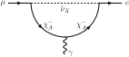
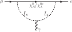
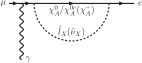
Figure 1: The four types of diagrams contributing to the photon interaction (3.1). All four diagrams contribute to the charge radius form factors $A_{1}^{\bar{e}\mu{\text{L}}/{\text{R}}}$; the first two also contribute to the dipole form factors $A_{2}^{\bar{e}\mu{\text{L}}/{\text{R}}}$.

We now discuss the MRSSM one-loop contributions to the required form factors and focus on the restrictions imposed by R-symmetry. The Feynman diagrams relevant for $\mu\to e\gamma$ are shown in Fig. 1; the diagrams for $a_{\mu}$ are analogous to the diagrams (a,b) with the replacement $e\to\mu$. We refer to table 2 for the pairs of particles which can couple to leptons without violation of R-charge conservation. Diagram (a) involves the exchange of a left-handed sneutrino and $\chi$-chargino, which involves the components $\tilde{W}$ and $\tilde{H}_{d}$. The couplings to the leptons involve the coupling coefficients $c$, which contain the gauge coupling $g_{2}$ and the lepton Yukawa couplings. Since there is no right-handed sneutrino, there is no Feynman diagram involving $\rho$-charginos. Diagram (b) in Fig. 1 involves the exchange of a slepton and a neutralino or an an antineutralino. In case of an antineutralino $\chi^{0c}_{A}$,the slepton must always be left-handed, see also Tab. 2. So the underlying physics of the antineutralino diagram is similar to the one of the chargino diagram; the involved couplings are $o$, which contain the gauge couplings $g_{2}$ and $g_{1}$ and the lepton Yukawa couplings. Diagram (b) with neutralino exchange involves the exchange of a right-handed slepton. Here the involved coupling coefficients are $n$, containing only $g_{1}$ and lepton Yukawa couplings. Diagrams (c,d) have a similar behaviour.

The MRSSM results for the constants $A_{1,2}^{\bar{e}\mu\,{\text{L}}/{\text{R}}}$ are decomposed as

$$A_{1}^{\bar{e}\mu{\text{L}}} =A_{1}^{n{\text{L}}}+A_{1}^{c{\text{L}}}\,,$$ (48)

$$A_{2}^{\bar{e}\mu{\text{L}}} =A_{2}^{n{\text{L}}}+A_{2}^{c{\text{L}}}\,,$$ (49)

$$A_{1}^{\bar{e}\mu{\text{R}}} =A_{1}^{n{\text{R}}}+A_{1}^{c{\text{R}}}\,,$$ (50)

$$A_{2}^{\bar{e}\mu{\text{R}}} =A_{2}^{n{\text{R}}}+A_{2}^{c{\text{R}}}\,,$$ (51)

into neutralino and chargino contributions. Using the dimensionless variables $x_{AX}^{n}\equiv m_{\chi^{0}_{A}}^{2}/m_{{\tilde{l}}_{X}}^{2}$ and $x_{AX}^{c}\equiv m^{2}_{\chi^{-}_{A}}/m^{2}_{{{\tilde{\nu}}}_{X}}$ and omitting terms which are suppressed by the electron Yukawa coupling, the charge radius contributions are given as

$$A_{1}^{n{\text{L}}} =\frac{1}{576\pi^{2}}\sum_{A,X}\Big{(}o^{{\text{L}}(l)\ast}_{1AX}o^{{\text{L}}(l)}_{2AX}+n^{{\text{L}}(l)\ast}_{1AX}n^{{\text{L}}(l)}_{2AX}\Big{)}\frac{1}{m_{{\tilde{l}}_{X}}^{2}}F_{0}^{n}(x_{AX}^{n})\,,$$ (52)

$$A_{1}^{n{\text{R}}} =\frac{1}{576\pi^{2}}\sum_{A,X}\Big{(}n^{{\text{R}}(l)\ast}_{1AX}n^{{\text{R}}(l)}_{2AX}+o^{{\text{R}}(l)\ast}_{1AX}o^{{\text{R}}(l)}_{2AX}\Big{)}\frac{1}{m_{{\tilde{l}}_{X}}^{2}}F_{0}^{n}(x_{AX}^{n})\,,$$ (53)

and

$$A_{1}^{c{\text{L}}} =-\frac{1}{576\pi^{2}}\sum_{A,X}c^{{\text{L}}(l)\ast}_{1AX}c^{{\text{L}}(l)}_{2AX}\frac{1}{m^{2}_{{\tilde{\nu}}_{X}}}F_{0}^{c}(x_{AX}^{c})\,,$$ (54)

$$A_{1}^{c{\text{R}}} =-\frac{1}{576\pi^{2}}\sum_{A,X}c^{{\text{R}}(l)\ast}_{1AX}c^{{\text{R}}(l)}_{2AX}\frac{1}{m^{2}_{{\tilde{\nu}}_{X}}}F_{0}^{c}(x_{AX}^{c})\,.$$ (55)

As shortly mentioned at the end of Sec. 2 the leading terms in Eqs. (52)–(55) are the $n^{\text{R}}$-, $o^{\text{L}}$-, and $c^{\text{L}}$-terms, which are from gaugino interactions; the other terms are suppressed by Yukawa couplings. Similar comments apply to the following results.

The dipole contributions from neutralinos/antineutralinos are given as

$$A_{2}^{n{\text{L}}} =\frac{1}{32\pi^{2}}\sum_{A,X}\frac{1}{m_{{\tilde{l}}_{X}}^{2}}\Big{\{}n^{{\text{R}}(l)\ast}_{1AX}n^{{\text{R}}(l)}_{2AX}F_{1}^{n}(x_{AX}^{n})+n^{{\text{R}}(l)\ast}_{1AX}n^{{\text{L}}(l)}_{2AX}\frac{m_{\chi^{0}_{A}}}{m_{\mu}}F_{2}^{n}(x_{AX}^{n})\Big{\}}$$

$$+\frac{1}{32\pi^{2}}\sum_{A,X}\frac{1}{m_{{\tilde{l}}_{X}}^{2}}\Big{\{}o^{{\text{R}}(l)\ast}_{1AX}o^{{\text{R}}(l)}_{2AX}F_{1}^{n}(x_{AX}^{n})+o^{{\text{R}}(l)\ast}_{1AX}o^{{\text{L}}(l)}_{2AX}\frac{m_{\chi^{0}_{A}}}{m_{\mu}}F_{2}^{n}(x_{AX}^{n})\Big{\}},$$ (56)

$$A_{2}^{n{\text{R}}} =\frac{1}{32\pi^{2}}\sum_{A,X}\frac{1}{m_{{\tilde{l}}_{X}}^{2}}\Big{\{}o^{{\text{L}}(l)\ast}_{1AX}o^{{\text{L}}(l)}_{2AX}F_{1}^{n}(x_{AX}^{n})+o^{{\text{L}}(l)\ast}_{1AX}o^{{\text{R}}(l)}_{2AX}\frac{m_{\chi^{0}_{A}}}{m_{\mu}}F_{2}^{n}(x_{AX}^{n})\Big{\}}$$

$$+\frac{1}{32\pi^{2}}\sum_{A,X}\frac{1}{m_{{\tilde{l}}_{X}}^{2}}\Big{\{}n^{{\text{L}}(l)\ast}_{1AX}n^{{\text{L}}(l)}_{2AX}F_{1}^{n}(x_{AX}^{n})+n^{{\text{L}}(l)\ast}_{1AX}n^{{\text{R}}(l)}_{2AX}\frac{m_{\chi^{0}_{A}}}{m_{\mu}}F_{2}^{n}(x_{AX}^{n})\Big{\}}\,.$$ (57)

The dipole contributions from charginos are given as

$$A_{2}^{c{\text{L}}} =-\frac{1}{32\pi^{2}}\sum_{A,X}\frac{1}{m^{2}_{{\tilde{\nu}}_{X}}}\Big{\{}c^{{\text{R}}(l)\ast}_{1AX}c^{{\text{R}}(l)}_{2AX}F_{1}^{c}(x_{AX}^{c})+c^{{\text{R}}(l)\ast}_{1AX}c^{{\text{L}}(l)}_{2AX}\frac{m_{\chi^{-}_{A}}}{m_{\mu}}F_{2}^{c}(x_{AX}^{c})\Big{\}}\,,$$ (58)

$$A_{2}^{c{\text{R}}} =-\frac{1}{32\pi^{2}}\sum_{A,X}\frac{1}{m^{2}_{{\tilde{\nu}}_{X}}}\Big{\{}c^{{\text{L}}(l)\ast}_{1AX}c^{{\text{L}}(l)}_{2AX}F_{1}^{c}(x_{AX}^{c})+c^{{\text{L}}(l)\ast}_{1AX}c^{{\text{R}}(l)}_{2AX}\frac{m_{\chi^{-}_{A}}}{m_{\mu}}F_{2}^{c}(x_{AX}^{c})\Big{\}}\,.$$ (59)

The MRSSM results for the contributions to $a_{\mu}$ are

$$a_{\mu}=a_{\mu}^{{\tilde{\chi}}^{-}}+a_{\mu}^{\tilde{\chi}^{0}}+a_{\mu}^{\tilde{\chi}^{0c}}\,,$$ (60)

with

$$a_{\mu}^{{\tilde{\chi}}^{-}}=\frac{1}{16\pi^{2}}\frac{m_{\mu}^{2}}{m_{{\tilde{\nu}}_{X}}^{2}}\Big{\{} (c^{{\text{L}}}_{2AX}c^{{\text{L}}\ast}_{2AX}+c^{{\text{R}}}_{2AX}c^{{\text{R}}\ast}_{2AX})F_{1}^{c}(x^{c}_{AX})$$

$$+\frac{m_{\tilde{\chi}^{-}_{A}}}{2m_{\mu}}(c^{{\text{L}}}_{2AX}c^{{\text{R}}\ast}_{2AX}+c^{{\text{R}}}_{2AX}c^{{\text{L}}\ast}_{2AX})F_{2}^{c}(x^{c}_{AX})\Big{\}}\,,$$ (61a)

$$a_{\mu}^{\tilde{\chi}^{0}}=\frac{-1}{16\pi^{2}}\frac{m_{\mu}^{2}}{m_{{\tilde{\mu}}_{X}}^{2}}\Big{\{} (n^{{\text{L}}}_{2AX}n^{{\text{L}}\ast}_{2AX}+n^{{\text{R}}}_{2AX}n^{{\text{R}}\ast}_{2AX})F_{1}^{n}(x^{n}_{AX})$$

$$+\frac{m_{\tilde{\chi}^{0}_{A}}}{2m_{\mu}}(n^{{\text{L}}}_{2AX}n^{{\text{R}}\ast}_{2AX}+n^{{\text{R}}}_{2AX}n^{{\text{L}}\ast}_{2AX})F_{2}^{n}(x^{n}_{AX})\Big{\}}\,,$$ (61b)

$$a_{\mu}^{\tilde{\chi}^{0c}}=\frac{-1}{16\pi^{2}}\frac{m_{\mu}^{2}}{m_{{\tilde{\mu}}_{X}}^{2}}\Big{\{} (o^{{\text{L}}}_{2AX}o^{{\text{L}}\ast}_{2AX}+o^{{\text{R}}}_{2AX}o^{{\text{R}}\ast}_{2AX})F_{1}^{n}(x^{n}_{AX})$$

$$+\frac{m_{\tilde{\chi}^{0}_{A}}}{2m_{\mu}}(o^{{\text{L}}}_{2AX}o^{{\text{R}}\ast}_{2AX}+o^{{\text{R}}}_{2AX}o^{{\text{L}}\ast}_{2AX})F_{2}^{n}(x^{n}_{AX})\Big{\}}\,.$$ (61c)

The appearing loop functions are defined as

$$F_{0}^{n}(x) =\frac{1}{(1-x)^{4}}(2-9x+18x^{2}-11x^{3}+6x^{3}\ln x)\,,$$ (62a)

$$F_{1}^{n}(x) =\frac{1}{6(1-x)^{4}}(1-6x+3x^{2}+2x^{3}-6x^{2}\ln x)\,,$$ (62b)

$$F_{2}^{n}(x) =\frac{1}{(1-x)^{3}}(1-x^{2}+2x\ln x)\,,$$ (62c)

$$F_{0}^{c}(x) =\frac{1}{(1-x)^{4}}(16-45x+36x^{2}-7x^{3}+6(2-3x)\ln x)\,,$$ (62d)

$$F_{1}^{c}(x) =\frac{1}{6(1-x)^{4}}(2+3x-6x^{2}+x^{3}+6x\ln x)\,,$$ (62e)

$$F_{2}^{c}(x) =\frac{1}{(1-x)^{3}}(-3+4x-x^{2}-2\ln x)\,.$$ (62f)

3.2 $\mu\to e$ conversion

The coherent $\mu\to e$ conversion in a muonic atom is related to the photon dipole interaction $A_{2}$ and the effective 4-fermion interaction between $\mu$–$e$ and the quarks $q$ in the respective nucleus. We use the precise evaluation of the $\mu\to e$ conversion rate of Ref. Kitano:2002mt , which defines the general effective Lagrangian

$${\cal L}_{\rm int}^{\text{Ref.\ \cite[cite]{\@@bibref{Authors Phrase1YearPhrase2}{Kitano:2002mt}{\@@citephrase{(}}{\@@citephrase{)}}}}} = +\frac{4G_{\rm F}}{\sqrt{2}}\left[m_{\mu}\bar{e}\sigma^{\mu\nu}\left(\mathbb{A}_{L}^{*}{\text{P}}_{\text{L}}+\mathbb{A}_{R}^{*}{\text{P}}_{\text{R}}\right)\mu F_{\mu\nu}+{\text{H.c.}}\right]$$

$$-\frac{G_{\rm F}}{\sqrt{2}}\sum_{q=u,d,s}\left[{\rule[-8.53581pt]{0.0pt}{28.45274pt}\ }\right.\left(g_{LS(q)}\bar{e}{\text{P}}_{\text{R}}\mu+g_{RS(q)}\bar{e}{\text{P}}_{\text{L}}\mu\right)\bar{q}q$$

$$\hskip 68.28644pt+\left(g_{LP(q)}\bar{e}{\text{P}}_{\text{R}}\mu+g_{RP(q)}\bar{e}{\text{P}}_{\text{L}}\mu\right)\bar{q}\gamma_{5}q$$

$$\hskip 68.28644pt+\left(g_{LV(q)}\bar{e}\gamma^{\mu}{\text{P}}_{\text{L}}\mu+g_{RV(q)}\bar{e}\gamma^{\mu}{\text{P}}_{\text{R}}\mu\right)\bar{q}\gamma_{\mu}q$$

$$\hskip 68.28644pt+\left(g_{LA(q)}\bar{e}\gamma^{\mu}{\text{P}}_{\text{L}}\mu+g_{RA(q)}\bar{e}\gamma^{\mu}{\text{P}}_{\text{R}}\mu\right)\bar{q}\gamma_{\mu}\gamma_{5}q$$

$$\hskip 68.28644pt+\ \frac{1}{2}\left(g_{LT(q)}\bar{e}\sigma^{\mu\nu}{\text{P}}_{\text{R}}\mu+g_{RT(q)}\bar{e}\sigma^{\mu\nu}{\text{P}}_{\text{L}}\mu\right)\bar{q}\sigma_{\mu\nu}q+{\rm h.c.}\left.{\rule[-8.53581pt]{0.0pt}{28.45274pt}\ }\right]\,,$$

where we have adapted the sign in front of the photon field to our definition of the gauge covariant derivative. In the MRSSM not all of the 4-fermion form factors are relevant. Like in the MSSM, the effective 4-fermion interaction is mainly generated by photon penguin, $Z$-penguin, and box diagrams. These only give rise to the vector-like form factors (up to terms suppressed by additional powers of Yukawa couplings).

For an extensive discussion of the $Z$-penguins in the context of the MSSM, see Refs. Arganda:2005ji ; Krauss:2013gya ; Abada:2014kba . Higgs-penguin diagrams have been discussed for the MSSM in Refs. Kitano:2003wn ; Cirigliano:2009bz ; Crivellin:2014cta ; they are negligible, except if the extra Higgs bosons are much lighter than the SUSY particles and if $\tan\beta$ is very large. Since we do not consider such a parameter scenario in the present paper, we neglect the Higgs penguins.

We write the generated effective interaction Lagrangian excluding dipole contributions in the form of Ref. Hisano:1995cp ,

$${\cal{L}}^{\text{Ref.\ \cite[cite]{\@@bibref{Authors Phrase1YearPhrase2}{Hisano:1995cp}{\@@citephrase{(}}{\@@citephrase{)}}}}}_{\text{eff}}= {}-e^{2}{\bar{e}}\gamma_{\alpha}\left(A_{1}^{{{\text{R}}}}{\text{P}}_{\text{R}}+A_{1}^{{{\text{L}}}}{\text{P}}_{\text{R}}\right)\mu\,\sum_{q=u,d}Q_{q}{\bar{q}}\gamma^{\alpha}q$$

$$+\frac{g^{2}_{Z}}{m^{2}_{Z}}\,{\bar{e}}\gamma^{\alpha}\left(A_{Z}^{{{\text{R}}}}{\text{P}}_{\text{R}}+A_{Z}^{{{\text{L}}}}{\text{P}}_{\text{L}}\right)\mu\,\sum_{q=u,d}\frac{Z^{\text{R}}_{q}+Z^{\text{L}}_{q}}{2}{\bar{q}}\gamma_{\alpha}q$$

$$+e^{2}\,{\bar{e}}\gamma^{\alpha}(A_{\text{box}}^{{{\text{R}}}}{}_{q}{\text{P}}_{\text{R}}+A_{\text{box}}^{{{\text{L}}}}{}_{q}{\text{P}}_{\text{L}})\mu\,\sum_{q=u,d}{\bar{q}}\gamma_{\alpha}q\,,$$ (64)

with coefficients for the $Z$-penguin and the box diagrams. Comparing this effective Lagrangian and the definition of the dipole coefficients in Eq. (3.1) with Eq. (3.2) gives the relations

$$\mathbb{A}_{L}^{*} =-\frac{\sqrt{2}\,e}{8\,G_{\text{F}}}A_{2}^{\bar{e}\mu{\text{L}}}\,,$$ (65)

$$\mathbb{A}_{R}^{*} =-\frac{\sqrt{2}\,e}{8\,G_{\text{F}}}A_{2}^{\bar{e}\mu{\text{R}}}\,,$$ (66)

$$g_{LV(q)} =\frac{\sqrt{2}}{G_{\text{F}}}\Big{(}e^{2}Q_{q}A_{1}^{{\text{L}}}-\frac{g^{2}_{Z}}{m^{2}_{Z}}\left(\frac{Z^{\text{R}}_{q}+Z^{\text{L}}_{q}}{2}\right)A_{Z}^{{\text{L}}}-e^{2}A_{\text{box}}^{{\text{L}}}{}_{q}\Big{)}\,,$$ (67)

$$g_{{RV(q)}} =\frac{\sqrt{2}}{G_{\text{F}}}\Big{(}e^{2}Q_{q}A_{1}^{{{\text{R}}}}-\frac{g^{2}_{Z}}{m^{2}_{Z}}\left(\frac{Z^{\text{R}}_{q}+Z^{\text{L}}_{q}}{2}\right)A_{Z}^{{\text{R}}}-e^{2}A_{\text{box}}^{{\text{R}}}{}_{q}\Big{)}\,.$$ (68)

With these relations we can define coefficients for protons and neutrons

$$\tilde{g}^{(p)}_{LV,RV}= 2g_{LV,RV(u)}+g_{LV,RV(d)}\,,$$ (69)

$$\tilde{g}^{(n)}_{LV,RV}= g_{LV,RV(u)}+2g_{LV,RV(d)}\,,$$ (70)

and obtain the $\mu\to e$ conversion rate and branching ratio as Kitano:2002mt

$$\omega_{\text{conv}} =2G_{\text{F}}^{2}\left|\mathbb{A}_{R}^{*}D+\tilde{g}^{(p)}_{LV}V^{(p)}+\tilde{g}^{(n)}_{LV}V^{(n)}\right|^{2}+L\leftrightarrow R\,,$$ (71)

$$B_{\mu N\to eN} =\frac{\omega_{\text{conv}}}{\omega_{\text{capt}}}\,,$$ (72)

where the constants $D$, $V^{(p,n)}$ correspond to overlap integrals evaluated in Ref. Kitano:2002mt . We will use numerical values specific for aluminum, where $D=0.0357$, $V^{(p)}=0.0159$, $V^{(n)}=0.0169$ in units of $m_{\mu}^{5/2}$. The capture rate for aluminium is $\omega_{\text{capt}}=0.7054\times 10^{6}/s=4.643\times 10^{-19}$ GeV Kitano:2002mt ; Suzuki:1987jf .

The up-to-date experimental upper limit is obtained for the gold nucleus from the SINDRUM experiment Bertl:2006up ,

$$B_{\mu\text{Au}\to e\text{Au}} <7\times 10^{-13}\ (90\%\text{ C.L.})\,.$$ (73)

In the forthcoming few years, the limit will be improved substantially by the COMET Cui:2009zz ; Kuno:2013mha and Mu2E Abrams:2012er experiments. Both of these experiments will measure $\mu\to e$ conversion in an aluminium nucleus. The foreseen limits are $7.2\times 10^{-15}$ for COMET Phase 1 and better than $10^{-16}$ for COMET Phase II and for Mu2e.

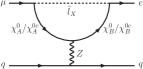
(a) Type 1 $A_{Z}^{n\,{\text{L}}/{\text{R}}\,(1)}$

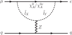
(b) Type 2 $A_{Z}^{n\,{\text{L}}/{\text{R}}\,(2)}$

(c) Type 3 $A_{Z}^{n\,{\text{L}}/{\text{R}}\,(3)}$

(d) Type 4 $A_{Z}^{n\,{\text{L}}/{\text{R}}\,(4)}$

Figure 2: The four types of $Z$-penguin diagrams corresponding to Eqs. (74). The chargino diagrams are analogous with the replacement of $\chi^{0}$ with $\chi^{-}$ and ${\tilde{l}}$ with $\tilde{\nu}$.

We now turn to the actual one-loop results in the MRSSM. The $Z$-penguin is given by the diagrams in Fig. 2. The diagrams can be first classified according to the exchanged particles: neutralinos and right-handed sleptons with couplings $n$, antineutralinos and left-handed sleptons with couplings $o$, and $\chi$-charginos and sneutrinos with couplings $c$. The diagrams can be further classified into diagrams with $Z$ coupling to the neutralino/chargino (diagram type 1), to the sfermion (type 2), and to the muon/electron (types 3, 4). Due to the Ward-like identity corresponding to broken gauge invariance the diagram types 2+3+4 exactly cancel in case of the (anti)neutralino diagrams and partially cancel in case of the chargino diagrams. The full contribution to the $Z$-penguin can thus be written as

$$A_{Z}^{{{\text{L}}}}= A_{Z}^{n{\text{L}}(1)}+A_{Z}^{n{\text{L}}(2)}+A_{Z}^{n{\text{L}}(3+4)}+A_{Z}^{c{\text{L}}(1)}+A_{Z}^{c{\text{L}}(2)}+A_{Z}^{c{\text{L}}(3+4)}\,,$$ (74a)

$$A_{Z}^{{{\text{R}}}}= A_{Z}^{n{\text{R}}(1)}+A_{Z}^{n{\text{R}}(2)}+A_{Z}^{n{\text{R}}(3+4)}+A_{Z}^{c{\text{R}}(1)}+A_{Z}^{c{\text{R}}(2)}+A_{Z}^{c{\text{R}}(3+4)}\,,$$ (74b)

where the $Z$-penguin neutralino contributions are

$$A_{Z}^{n{\text{L}}(1)}= \frac{1}{16\pi^{2}}\sum_{A,B,X}n^{{\text{L}}(l)\ast}_{1BX}n^{{\text{L}}(l)}_{2AX}\Big{\{}-2F_{2}^{Z}(m^{2}_{\chi^{0}_{A}},m^{2}_{\chi^{0}_{B}},m^{2}_{{{\tilde{l}}_{X}}})\Big{(}\frac{-N^{2\ast}_{B3}N^{2}_{A3}+N^{2\ast}_{B4}N^{2}_{A4}}{2}\Big{)}$$

$$+m_{\chi^{0}_{A}}m_{\chi^{0}_{B}}F_{1}^{Z}(m^{2}_{\chi^{0}_{A}},m^{2}_{\chi^{0}_{B}},m^{2}_{{\tilde{l}}_{X}})\Big{(}\frac{-N^{1}_{B3}N^{1\ast}_{A3}+N^{1}_{B4}N^{1\ast}_{A4}}{2}\Big{)}\Big{\}}$$

$$+\frac{1}{16\pi^{2}}\sum_{A,B,X}o^{{\text{L}}(l)\ast}_{1BX}o^{{\text{L}}(l)}_{2AX}\Big{\{}-2F_{2}^{Z}(m^{2}_{\chi^{0}_{A}},m^{2}_{\chi^{0}_{B}},m^{2}_{{\tilde{l}}_{X}})\Big{(}\frac{N^{1\ast}_{B3}N^{1}_{A3}-N^{1\ast}_{B4}N^{1}_{A4}}{2}\Big{)}$$

$$+m_{\chi^{0}_{A}}m_{\chi^{0}_{B}}F_{1}^{Z}(m^{2}_{\chi^{0}_{A}},m^{2}_{\chi^{0}_{B}},m^{2}_{{\tilde{l}}_{X}})\Big{(}\frac{N^{2}_{B3}N^{2\ast}_{A3}-N^{2}_{B4}N^{2\ast}_{A4}}{2}\Big{)}\Big{\}}\,,$$ (75)

$$A_{Z}^{n{\text{R}}(1)}= \frac{1}{16\pi^{2}}\sum_{A,B,X}n^{{\text{R}}(l)\ast}_{1BX}n^{{\text{R}}(l)}_{2AX}\Big{\{}-2F_{2}^{Z}(m^{2}_{\chi^{0}_{A}},m^{2}_{\chi^{0}_{B}},m^{2}_{{\tilde{l}}_{X}})\Big{(}\frac{-N^{1}_{B3}N^{1\ast}_{A3}+N^{1}_{B4}N^{1\ast}_{A4}}{2}\Big{)}$$

$$+m_{\chi^{0}_{A}}m_{\chi^{0}_{B}}F_{1}^{Z}(m^{2}_{\chi^{0}_{A}},m^{2}_{\chi^{0}_{B}},m^{2}_{{\tilde{l}}_{X}})\Big{(}\frac{-N^{2\ast}_{B3}N^{2}_{A3}+N^{2\ast}_{B4}N^{2}_{A4}}{2}\Big{)}\Big{\}}$$

$$+\frac{1}{16\pi^{2}}\sum_{A,B,X}o^{{\text{R}}(l)\ast}_{1BX}o^{{\text{R}}(l)}_{2AX}\Big{\{}-2F_{2}^{Z}(m^{2}_{\chi^{0}_{A}},m^{2}_{\chi^{0}_{B}},m^{2}_{{\tilde{l}}_{X}})\Big{(}\frac{N^{2}_{B3}N^{2\ast}_{A3}-N^{2}_{B4}N^{2\ast}_{A4}}{2}\Big{)}$$

$$+m_{\chi^{0}_{A}}m_{\chi^{0}_{B}}F_{1}^{Z}(m^{2}_{\chi^{0}_{A}},m^{2}_{\chi^{0}_{B}},m^{2}_{{\tilde{l}}_{X}})\Big{(}\frac{N^{1\ast}_{B3}N^{1}_{A3}-N^{1\ast}_{B4}N^{1}_{A4}}{2}\Big{)}\Big{\}}\,,$$ (76)

$$A_{Z}^{n{\text{L}}(2)}= \frac{1}{16\pi^{2}}\sum_{A,X}\Big{\{}\big{(}n^{{\text{L}}(l)\ast}_{1AY}n^{{\text{L}}(l)}_{2AX}+o^{{\text{L}}(l)\ast}_{1AY}o^{{\text{L}}(l)}_{2AX}\big{)}\big{(}-2F_{2}^{Z}(m^{2}_{\chi^{0}_{A}},m^{2}_{{\tilde{l}}_{X}},m^{2}_{{\tilde{l}}_{Y}})\big{)}$$

$$\times\Big{[}\sum_{g=1}^{3}U^{{\tilde{l}}}_{Yg}U^{{\tilde{l}}\ast}_{Xg}Z^{{\text{L}}}_{l}+U^{{\tilde{l}}}_{Y(g+3)}U^{{\tilde{l}}\ast}_{X(g+3)}Z^{{\text{R}}}_{l}\Big{]}\Big{\}}\,,$$ (77)

$$A_{Z}^{n{\text{R}}(2)}= \frac{1}{16\pi^{2}}\sum_{A,X}\Big{\{}\big{(}n^{{\text{R}}(l)\ast}_{1AY}n^{{\text{R}}(l)}_{2AX}+o^{{\text{R}}(l)\ast}_{1AY}o^{{\text{R}}(l)}_{2AX}\big{)}\big{(}-2F_{2}^{Z}(m^{2}_{\chi^{0}_{A}},m^{2}_{{\tilde{l}}_{X}},m^{2}_{{\tilde{l}}_{Y}})\big{]}$$

$$\times\Big{[}\sum_{g=1}^{3}U^{{\tilde{l}}}_{Yg}U^{{\tilde{l}}\ast}_{Xg}Z^{{\text{L}}}_{l}+U^{{\tilde{l}}}_{Y(g+3)}U^{{\tilde{l}}\ast}_{X(g+3)}Z^{{\text{R}}}_{l}\Big{]}\Big{\}}\,,$$ (78)

$$A_{Z}^{n{\text{L}}(3+4)}= \frac{1}{16\pi^{2}}\sum_{A,X}\big{(}n^{{\text{L}}(l)\ast}_{1AX}n^{{\text{L}}(l)}_{2AX}+o^{{\text{L}}(l)\ast}_{1AX}o^{{\text{L}}(l)}_{2AX}\big{)}f_{2}^{Z}(m^{2}_{\chi^{0}_{A}},m^{2}_{{\tilde{l}}_{X}})Z^{{\text{L}}}_{l},$$ (79)

$$A_{Z}^{n{\text{R}}(3+4)}= \frac{1}{16\pi^{2}}\sum_{A,X}\big{(}n^{{\text{R}}(l)\ast}_{1AX}n^{{\text{R}}(l)}_{2AX}+o^{{\text{R}}(l)\ast}_{1AX}o^{{\text{R}}(l)}_{2AX}\big{)}f_{2}^{Z}(m^{2}_{\chi^{0}_{A}},m^{2}_{{\tilde{l}}_{X}})Z^{{\text{R}}}_{l}\,,$$ (80)

where $Z^{{\text{L}}}_{l}=-\frac{1}{2}+\sin^{2}\theta_{W}$ and $Z^{{\text{R}}}_{l}=\sin^{2}\theta_{W}$ as given in Eq. (12).

The $Z$-penguin chargino contributions are given by

$$A_{Z}^{c{\text{L}}(1)}= \frac{1}{16\pi^{2}}\sum_{A,B,X}c^{{\text{L}}(l)\ast}_{1BX}c^{{\text{L}}(l)}_{2AX}\Big{\{}-2F_{2}^{Z}(m^{2}_{\chi^{-}_{A}},m^{2}_{\chi^{-}_{B}},m^{2}_{{\tilde{\nu}}_{X}})$$

$$\qquad\times\big{\{}-V^{1\ast}_{B1}V^{1}_{A1}-\frac{1}{2}V^{1\ast}_{B2}V^{1}_{A2}+s^{2}_{\text{W}}\delta_{AB}\big{\}}$$

$$+m_{\chi^{-}_{A}}m_{\chi^{-}_{B}}F_{1}^{Z}(m^{2}_{\chi^{-}_{A}},m^{2}_{\chi^{-}_{B}},m^{2}_{{\tilde{\nu}}_{X}})\big{\{}-U^{1}_{B1}U^{1\ast}_{A1}-\frac{1}{2}U^{1}_{B2}U^{1\ast}_{A2}+s^{2}_{\text{W}}\delta_{AB}\big{\}}\Big{\}}\,,$$ (81)

$$A_{Z}^{c{\text{R}}(1)}= \frac{1}{16\pi^{2}}\sum_{A,B,X}c^{{\text{R}}(l)\ast}_{1BX}c^{{\text{R}}(l)}_{2AX}\Big{\{}-2F_{2}^{Z}(m^{2}_{\chi^{-}_{A}},m^{2}_{\chi^{-}_{B}},m^{2}_{{\tilde{\nu}}_{X}})$$

$$\qquad\times\big{\{}-U^{1}_{B1}U^{1\ast}_{A1}-\frac{1}{2}U^{1}_{B2}U^{1\ast}_{A2}+s^{2}_{\text{W}}\delta_{AB}\big{\}}$$

$$+m_{\chi^{-}_{A}}m_{\chi^{-}_{B}}F_{1}^{Z}(m^{2}_{\chi^{-}_{A}},m^{2}_{\chi^{-}_{B}},m^{2}_{{\tilde{\nu}}_{X}})\big{\{}-V^{1\ast}_{B1}V^{1}_{A1}-\frac{1}{2}V^{1\ast}_{B2}V^{1}_{A2}+s^{2}_{\text{W}}\delta_{AB}\big{\}}\Big{\}}\,,$$ (82)

$$A_{Z}^{c{\text{L}}(2)}= \frac{1}{16\pi^{2}}\sum_{A,X,Y}c^{{\text{L}}(l)\ast}_{1AY}c^{{\text{L}}(l)}_{2AX}\big{(}-2F_{2}^{Z}(m^{2}_{\chi^{-}_{A}},m^{2}_{{\tilde{\nu}}_{X}},m^{2}_{{\tilde{\nu}}_{Y}})\big{)}$$

$$\times\Big{[}\sum_{g=1}^{3}U^{{\tilde{\nu}}}_{Yg}U^{{\tilde{\nu}}\ast}_{Xg}Z^{{\text{L}}}_{\nu}+U^{{\tilde{\nu}}}_{Y(g+3)}U^{{\tilde{\nu}}\ast}_{X(g+3)}Z^{{\text{R}}}_{\nu}\Big{]}\,,$$ (83)

$$A_{Z}^{c{\text{R}}(2)}= \frac{1}{16\pi^{2}}\sum_{A,X,Y}c^{{\text{R}}(l)\ast}_{1AY}c^{{\text{R}}(l)}_{2AX}\big{(}-2F_{2}^{Z}(m^{2}_{\chi^{-}_{A}},m^{2}_{{\tilde{\nu}}_{X}},m^{2}_{{\tilde{\nu}}_{Y}})\big{)}$$

$$\times\Big{[}\sum_{g=1}^{3}U^{{\tilde{\nu}}}_{Yg}U^{{\tilde{\nu}}\ast}_{Xg}Z^{{\text{L}}}_{\nu}+U^{{\tilde{\nu}}}_{Y(g+3)}U^{{\tilde{\nu}}\ast}_{X(g+3)}Z^{{\text{R}}}_{\nu}\Big{]}\,,$$ (84)

$$A_{Z}^{c{\text{L}}(3+4)}= \frac{1}{16\pi^{2}}\sum_{A,X}c^{{\text{L}}(l)\ast}_{1AX}c^{{\text{L}}(l)}_{2AX}\big{(}f_{2}^{Z}(m^{2}_{\chi^{-}_{A}},m^{2}_{{\tilde{\nu}}_{X}})Z^{{\text{L}}}_{l}\big{)}\,,$$ (85)

$$A_{Z}^{c{\text{R}}(3+4)}= \frac{1}{16\pi^{2}}\sum_{A,X}c^{{\text{R}}(l)\ast}_{1AX}c^{{\text{R}}(l)}_{2AX}\big{(}f_{2}^{Z}(m^{2}_{\chi^{-}_{A}},m^{2}_{{\tilde{\nu}}_{X}})Z^{{\text{R}}}_{l}\big{)}\,,$$ (86)

where again $Z^{{\text{L}}}_{l}=-\frac{1}{2}+\sin^{2}\theta_{W}$ and $Z^{{\text{R}}}_{l}=\sin^{2}\theta_{W}$, while $Z^{{\text{L}}}_{\nu}=\frac{1}{2}$ and $Z^{{\text{R}}}_{\nu}=0$.

The loop functions needed for the $Z$-penguin contributions are the ones defined in Ref. Ilakovac:2012sh ,

$$F_{1}^{Z}(a,b,c) =-\frac{1}{b-c}\Big{(}\frac{a\ln a-b\ln b}{a-b}-\frac{a\ln a-c\ln c}{a-c}\Big{)}\,,$$ (87)

$$F_{2}^{Z}(a,b,c) =\frac{3}{8}-\frac{1}{4(b-c)}\Big{(}\frac{a^{2}\ln a-b^{2}\ln b}{a-b}-\frac{a^{2}\ln a-c^{2}\ln c}{a-c}\Big{)}\,,$$ (88)

$$f_{2}^{Z}(a,b) =\frac{1}{2}-\frac{\ln b}{2}+\frac{a^{2}-b^{2}+2a^{2}(\ln b-\ln a)}{4(a-b)^{2}}\,.$$ (89)

The two loop functions $F_{1}^{Z}(a,b,c)$ and $F_{2}^{Z}(a,b,c)$ are totally symmetric; the loop function $f_{2}^{Z}(a,b)$ is not symmetric.

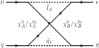
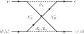
Figure 3: Box diagrams with neutralinos/antineutralinos and charginos. All indicated particles run in the direction of the arrows/from left to right.

The box diagrams are shown in Fig. 3. The results for the neutralino box diagrams are

$${A_{\text{box}}^{n{\text{L}}}}_{q_{g}} =\frac{1}{8e^{2}}\sum_{A,B,X,Y}\Big{\{}J_{4}(m_{\chi^{0}_{A}},m_{\chi^{0}_{B}},m_{{\tilde{q}}_{Y}},m_{{\tilde{l}}_{X}})$$

$$\times\Big{(}(o^{{\text{L}}(l)\ast}_{1BX}o^{{\text{L}}(l)}_{2AX}o^{{\text{L}}(q)\ast}_{gAY}o^{{\text{L}}(q)}_{gBY}+n^{{\text{L}}(l)\ast}_{1BX}n^{{\text{L}}(l)}_{2AX}n^{{\text{L}}(q)\ast}_{gAY}n^{{\text{L}}(q)}_{gBY})$$

$$-(o^{{\text{L}}(l)\ast}_{1BX}o^{{\text{L}}(l)}_{2AX}n^{{\text{R}}(q)\ast}_{gAY}n^{{\text{R}}(q)}_{gBY}+n^{{\text{L}}(l)\ast}_{1BX}n^{{\text{L}}(l)}_{2AX}o^{{\text{R}}(q)\ast}_{gAY}o^{{\text{R}}(q)}_{gBY})\Big{)}\Big{\}}$$

$$-\frac{1}{4e^{2}}\sum_{A,B,X,Y}\Big{\{}m_{\chi^{0}_{A}}m_{\chi^{0}_{B}}I_{4}(m_{\chi^{0}_{A}},m_{\chi^{0}_{B}},m_{{\tilde{q}}_{Y}},m_{{\tilde{l}}_{X}})$$

$$\times\Big{(}(o^{{\text{L}}(l)\ast}_{1BX}o^{{\text{L}}(l)}_{2AX}o^{{\text{R}}(q)}_{gAY}o^{{\text{R}}(q)\ast}_{gBY}+n^{{\text{L}}(l)\ast}_{1BX}n^{{\text{L}}(l)}_{2AX}n^{{\text{R}}(q)\ast}_{gAY}n^{{\text{R}}(q)}_{gBY})$$

$$-(o^{{\text{L}}(l)\ast}_{1BX}o^{{\text{L}}(l)}_{2AX}n^{{\text{L}}(q)}_{gAY}n^{{\text{L}}(q)\ast}_{gBY}+n^{{\text{L}}(l)\ast}_{1BX}n^{{\text{L}}(l)}_{2AX}o^{{\text{L}}(q)}_{gAY}o^{{\text{L}}(q)\ast}_{gBY})\Big{)}\Big{\}}\,,$$ (90)

$${A_{\text{box}}^{n{\text{R}}}}_{q_{g}} =\frac{1}{8e^{2}}\sum_{A,B,X,Y}\Big{\{}J_{4}(m_{\chi^{0}_{A}},m_{\chi^{0}_{B}},m_{{\tilde{q}}_{Y}},m_{{\tilde{l}}_{X}})$$

$$\times\Big{(}(n^{{\text{R}}(l)\ast}_{1BX}n^{{\text{R}}(l)}_{2AX}n^{{\text{R}}(q)\ast}_{gAY}n^{{\text{R}}(q)}_{gBY}+o^{{\text{R}}(l)\ast}_{1BX}o^{{\text{R}}(l)}_{2AX}o^{{\text{R}}(q)\ast}_{gAY}o^{{\text{R}}(q)}_{gBY})$$

$$-(n^{{\text{R}}(l)\ast}_{1BX}n^{{\text{R}}(l)}_{2AX}o^{{\text{L}}(q)\ast}_{gAY}o^{{\text{L}}(q)}_{gBY}+o^{{\text{R}}(l)\ast}_{1BX}o^{{\text{R}}(l)}_{2AX}n^{{\text{L}}(q)\ast}_{gAY}n^{{\text{L}}(q)}_{gBY})\Big{)}\Big{\}}$$

$$-\frac{1}{4e^{2}}\sum_{A,B,X,Y}\Big{\{}m_{\chi^{0}_{A}}m_{\chi^{0}_{B}}I_{4}(m_{\chi^{0}_{A}},m_{\chi^{0}_{B}},m_{{\tilde{q}}_{Y}},m_{{\tilde{l}}_{X}})$$

$$\times\Big{(}(o^{{\text{R}}(l)\ast}_{1BX}o^{{\text{R}}(l)}_{2AX}o^{{\text{L}}(q)}_{gAY}o^{{\text{L}}(q)\ast}_{gBY}+n^{{\text{R}}(l)\ast}_{1BX}n^{{\text{R}}(l)}_{2AX}n^{{\text{L}}(q)\ast}_{gAY}n^{{\text{L}}(q)}_{gBY})$$

$$-(o^{{\text{R}}(l)\ast}_{1BX}o^{{\text{R}}(l)}_{2AX}n^{{\text{R}}(q)}_{gAY}n^{{\text{R}}(q)\ast}_{gBY}+n^{{\text{R}}(l)\ast}_{1BX}n^{{\text{R}}(l)}_{2AX}o^{{\text{R}}(q)}_{gAY}o^{{\text{R}}(q)\ast}_{gBY})\Big{)}\Big{\}}\,.$$ (91)

The chargino box diagram contributions are

$${A_{\text{box}}^{c{\text{L}}}}_{u} =\frac{1}{e^{2}}\sum_{A,B,X,Y}\Big{\{}-\frac{1}{8}J_{4}(m_{\chi^{-}_{A}},m_{\chi^{-}_{B}},m_{\tilde{d}_{Y}},m_{{\tilde{l}}_{X}})c^{{\text{L}}(l)\ast}_{1BX}c^{{\text{L}}(l)}_{2AX}c^{{\text{L}}(u)\ast}_{1AY}c^{{\text{L}}(u)}_{1BY}$$

$$+\frac{1}{4}m_{\chi^{-}_{A}}m_{\chi^{-}_{B}}I_{4}(m_{\chi^{-}_{A}},m_{\chi^{-}_{B}},m_{\tilde{d}_{Y}},m_{{\tilde{l}}_{X}})c^{{\text{L}}(l)\ast}_{1BX}c^{{\text{L}}(l)}_{2AX}c^{{\text{R}}(u)\ast}_{1AY}c^{{\text{R}}(u)}_{1BY}\Big{\}}\,,$$ (92)

$${A_{\text{box}}^{c{\text{R}}}}_{u} =\frac{1}{e^{2}}\sum_{A,B,X,Y}\Big{\{}-\frac{1}{8}J_{4}(m_{\chi^{-}_{A}},m_{\chi^{-}_{B}},m_{\tilde{d}_{Y}},m_{{\tilde{l}}_{X}})c^{{\text{R}}(l)\ast}_{1BX}c^{{\text{R}}(l)}_{2AX}c^{{\text{R}}(u)\ast}_{1AY}c^{{\text{R}}(u)}_{1BY}$$

$$+\frac{1}{4}m_{\chi^{-}_{A}}m_{\chi^{-}_{B}}I_{4}(m_{\chi^{-}_{A}},m_{\chi^{-}_{B}},m_{\tilde{d}_{Y}},m_{{\tilde{l}}_{X}})c^{{\text{R}}(l)\ast}_{1BX}c^{{\text{R}}(l)}_{2AX}c^{{\text{L}}(u)\ast}_{1AY}c^{{\text{L}}(u)}_{1BY}\Big{\}}\,,$$ (93)

$${A_{\text{box}}^{c{\text{L}}}}_{d} =\frac{1}{e^{2}}\sum_{A,B,X,Y}\Big{\{}\frac{1}{8}J_{4}(m_{\chi^{-}_{A}},m_{\chi^{-}_{B}},m_{\tilde{u}_{Y}},m_{{\tilde{l}}_{X}})c^{{\text{L}}(l)\ast}_{1BX}c^{{\text{L}}(l)}_{2AX}c^{{\text{L}}(d)\ast}_{1AY}c^{{\text{L}}(d)}_{1BY}$$

$$-\frac{1}{4}m_{\chi^{-}_{A}}m_{\chi^{-}_{B}}I_{4}(m_{\chi^{-}_{A}},m_{\chi^{-}_{B}},m_{\tilde{u}_{Y}},m_{{\tilde{l}}_{X}})c^{{\text{L}}(l)\ast}_{1BX}c^{{\text{L}}(l)}_{2AX}c^{{\text{R}}(d)\ast}_{1AY}c^{{\text{R}}(d)}_{1BY}\Big{\}}\,,$$ (94)

$${A_{\text{box}}^{c{\text{R}}}}_{d} =\frac{1}{e^{2}}\sum_{A,B,X,Y}\Big{\{}\frac{1}{8}J_{4}(m_{\chi^{-}_{A}},m_{\chi^{-}_{B}},m_{\tilde{u}_{Y}},m_{{\tilde{l}}_{X}})c^{{\text{R}}(l)\ast}_{1BX}c^{{\text{R}}(l)}_{2AX}c^{{\text{R}}(d)\ast}_{1AY}c^{{\text{R}}(d)}_{1BY}$$

$$-\frac{1}{4}m_{\chi^{-}_{A}}m_{\chi^{-}_{B}}I_{4}(m_{\chi^{-}_{A}},m_{\chi^{-}_{B}},m_{\tilde{u}_{Y}},m_{{\tilde{l}}_{X}})c^{{\text{R}}(l)\ast}_{1BX}c^{{\text{R}}(l)}_{2AX}c^{{\text{L}}(d)\ast}_{1AY}c^{{\text{L}}(d)}_{1BY}\Big{\}}\,.$$ (95)

Here the following loop functions appear:

$$I_{4}(a,b,c,d) =\frac{1}{16\pi^{2}}\Big{\{}\frac{a^{2}\ln\frac{a^{2}}{d^{2}}}{(a^{2}-b^{2})(a^{2}-c^{2})(d^{2}-a^{2})}-\frac{b^{2}\ln\frac{b^{2}}{d^{2}}}{(a^{2}-b^{2})(b^{2}-c^{2})(d^{2}-b^{2})}$$

$$+\frac{c^{2}\ln\frac{c^{2}}{d^{2}}}{(a^{2}-c^{2})(b^{2}-c^{2})(d^{2}-c^{2})}\Big{\}}\,,$$ (96)

$$J_{4}(a,b,c,d) =\frac{1}{16\pi^{2}}\Big{\{}\frac{a^{4}\frac{a^{2}}{d^{2}}}{(a^{2}-b^{2})(a^{2}-c^{2})(d^{2}-a^{2})}-\frac{b^{4}\frac{b^{2}}{d^{2}}}{(a^{2}-b^{2})(b^{2}-c^{2})(d^{2}-b^{2})}$$

$$+\frac{c^{4}\frac{c^{2}}{d^{2}}}{(a^{2}-c^{2})(b^{2}-c^{2})(d^{2}-c^{2})}\Big{\}}\,.$$ (97)

4 Numerical results

4.1 Relevant parameters and experimental constraints

We begin our discussion of the numerical results with a survey of the relevant MRSSM parameters, an overview of characteristic regions of parameter space, and a discussion of applicable experimental constraints on the parameters. The three observables $a_{\mu}$, $\mu\to e\gamma$ and $\mu\to e$ depend on an increasing number of parameters. $a_{\mu}$ depends only (up to small effects due to mixing) on the masses of the gauginos and down-type Higgsinos and thus on the parameters

$$M_{B}^{D},\,M_{W}^{D},\,\mu_{d},\,\lambda_{d},\,\Lambda_{d}$$ (98)

as well as on the slepton mass parameters

$$m_{\tilde{l},22},\,m_{\tilde{e},22}.$$ (99)

The dependence on the up-type Higgsino mass $\mu_{u}$ and on $\tan\beta$ is very weak, in contrast to the MSSM.

The observable $\mu\to e\gamma$ only depends on photon dipole operators and has thus a similar parameter dependence as $a_{\mu}$, but it involves slepton mass and mixing parameters of the first and second generation. We use the common dimensionless LFV parameters

$$\delta^{{\text{L}}}_{12} \equiv\frac{(m_{\tilde{l}}^{2})_{12}}{m_{\tilde{l},11}\,m_{\tilde{l},22}} \delta^{{\text{R}}}_{12} \equiv\frac{(m_{\tilde{e}}^{2})_{12}}{m_{\tilde{e},11}\,m_{\tilde{e},22}}\,.$$ (100)

Furthermore, we keep the ratio of the slepton masses around order 1 and set always the selectron masses to $1.5$ times the corresponding smuon masses,

$$m_{\tilde{l},11} =1.5\,m_{\tilde{l},22}\,, m_{\tilde{e},11} =1.5\,m_{\tilde{e},22}\,.$$ (101)

This is not a significant restriction. We have explicitly checked that the phenomenological results presented below remain essentially the same if the factor $1.5$ is changed to a factor $1$ or anything of the order 1. Indeed the LFV observables mainly depend on the dimensionless parameters $\delta_{12}^{{\text{L}},{\text{R}}}$, unless there is a significant hierarchy between the different slepton masses, in which case the observables are simply suppressed by the heavier mass scale.

The muon-to-electron conversion $\mu\to e$ depends on additional types of diagrams and thus on additional parameters. The $Z$-penguin diagrams have a significant dependence also on the up-type Higgsino parameters and $\tan\beta$

$$\mu_{u},\,\lambda_{u},\,\Lambda_{u},\,\tan\beta,$$ (102)

and the box diagrams depend on the squark masses. For simplicity we choose a common squark mass scale without squark flavour mixing,

$$(m_{\tilde{q}}^{2})_{ij}=(m_{\tilde{u}}^{2})_{ij}=(m_{\tilde{d}}^{2})_{ij}\equiv\delta_{ij}m_{\tilde{q}}^{2}\,.$$ (103)

The parameter space can be best explored by investigating various different parameter scenarios, corresponding to distinct patterns of hierarchies between light/heavy SUSY particles. In this way we can isolate several parameter influences, separate leading and subleading terms and obtain a complete understanding of the parameter dependence. In the MSSM, corresponding parameter scenarios have been defined e.g. in Refs. Moroi:1995yh ; Cho:2011rk ; DSreview ; Fargnoli:2013zia for studies of $a_{\mu}$ and in Refs. Kersten:2014xaa ; CalibbiShadmi for LFV observables.

All Feynman diagrams for the considered observables involve the exchange of at least one neutralino/chargino and one slepton/sneutrino, and all diagrams have a generic $1/m_{\text{SUSY}}^{2}$ mass suppression. Hence we need at least two light SUSY particles in order to have non-negligible results: at least one neutralino/chargino and at least one slepton/sneutrino. In addition, at least one light neutralino/chargino must be gaugino-like since otherwise all contributions are suppressed by additional powers of Yukawa couplings.

Hence we end up with seven distinct parameter scenarios with characteristic mass hierarchies, which we denote as BL, BR, WL, BHL, BHR, WHL, equal-mass. To be concrete, we define the following patterns:

BL: $$M_{B}^{D}= m_{\text{SUSY}}, m_{\tilde{l},{22}}= (1\ldots 1.5)\times m_{\text{SUSY}}, \lambda_{d},\,\delta^{{\text{L}}}_{12}= \text{free},$$ (104a)

BR: $$M_{B}^{D}= m_{\text{SUSY}}, m_{\tilde{e},{22}}= (1\ldots 1.5)\times m_{\text{SUSY}}, \lambda_{d},\,\delta^{{\text{R}}}_{12}= \text{free},$$ (104b)

WL: $$M_{W}^{D}= m_{\text{SUSY}}, m_{\tilde{l},{22}}= (1\ldots 1.5)\times m_{\text{SUSY}}, \Lambda_{d},\,\delta^{{\text{L}}}_{12}= \text{free},$$ (104c)

BHL: $$M_{B}^{D}=\mu_{d}= m_{\text{SUSY}}, m_{\tilde{l},{22}}= (1\ldots 1.5)\times m_{\text{SUSY}}, \lambda_{d},\,\delta^{{\text{L}}}_{12}= \text{free},$$ (104d)

BHR: $$M_{B}^{D}=\mu_{d}= m_{\text{SUSY}}, m_{\tilde{e},{22}}= (1\ldots 1.5)\times m_{\text{SUSY}}, \lambda_{d},\,\delta^{{\text{R}}}_{12}= \text{free},$$ (104e)

WHL: $$M_{W}^{D}=\mu_{d}= m_{\text{SUSY}}, m_{\tilde{l},{22}}= (1\ldots 1.5)\times m_{\text{SUSY}}, \Lambda_{d},\,\delta^{{\text{L}}}_{12}= \text{free},$$ (104f)

as well as

equal-mass: $$M_{B}^{D}=M_{W}^{D}=\mu_{d}= m_{\text{SUSY}}, m_{\tilde{l},{22}}=m_{\tilde{e},{22}}= (1\ldots 1.5)\times m_{\text{SUSY}},$$

$$\lambda_{d},\,\Lambda_{d},\,\delta^{{\text{L}}}_{12},\,\delta^{{\text{R}}}_{12}= \text{free}.$$ (104g)

In each scenario of Eq. (104), all other masses not listed in the corresponding equation are set to very high values (in practice we choose $50$ TeV). Unless noted otherwise, the other, not listed $\lambda_{i},\Lambda_{i}$ and $\delta^{i}_{12}$ are set to zero, and $\tan\beta$ is set to $\tan\beta=40$; a standard value for the non-vanishing flavour mixings $\delta^{{\text{L}},{\text{R}}}_{12}=10^{-4}$ is chosen. We also always set the selectron masses as given in Eq. (101).

Thus each scenario is then characterized by one common mass scale $m_{\text{SUSY}}$. The BL, BR, WL regions contain only two light masses (one gaugino and one smuon). The parameter dependence in these scenario is particularly simple as mainly gauge couplings enter. The three further scenarios BHL, BHR, WHL with a light Higgsino show a more interesting parameter dependence; enhancements driven by $\lambda_{d}$ and $\Lambda_{d}$ become possible. The equal-mass case contains interferences between different contributions.

Now we turn to constraints on the relevant parameters from existing data. The SUSY masses are constrained by direct collider searches at LEP, Tevatron and LHC. There is a multitude of analyses of collider searches for different assumptions on the SUSY spectrum. For our purposes, the most conservative and robust bounds are the most important. They correspond to assuming small mass splittings between SUSY particles, i.e. compressed SUSY spectra such as the ones in Eq. (104). As we will see, these are the spectra which maximize the contributions to the observables studied in the present paper. The bounds on the relevant particle masses under the assumption of small mass splittings are PDG

$$m_{\chi^{\pm}_{1}} >92\text{ GeV} m_{\tilde{\mu}_{\text{R}}} >94\text{ GeV}\,.$$ (105)

Since these limits originate from kinematics, they apply equally to the MSSM and the MRSSM. For a recast of more model-dependent chargino limits to the MRSSM see Ref. Diessner:2015iln ; this reference also confirms that the limits become as weak as in Eq. (105) in case of compressed spectra.

The LHC limits from chargino and neutralino searches do not apply for our case of very compressed chargino and neutralino masses. However, limits from slepton searches are relevant. Up-to-date limits from Refs. PDG ; Aaboud:2017leg ; ATLAS-CONF-2019-008 show that certain mass splittings $\Delta m(\tilde{l}_{1},\chi^{0}_{1})$ are allowed: e.g. for $m_{\chi^{0}_{1}}$ around $100$ GeV, mass splittings between below $1$ GeV and between $20\ldots 60$ GeV are allowed, while other mass splittings are excluded under certain assumptions: mass degeneracy of all sleptons of the first and second generation and $100\%$ branching ratio of slepton decays into $\chi^{0}_{1}$, which are not fulfilled in our scenarios. As a result, our choice of varying the slepton masses in the range $(1\ldots 1.5)\times m_{\text{SUSY}}$ in the scenarios (104) is subject to these exclusion limits, and we expect that a fraction of data points in our plots might be excluded by LHC limits. However, the most interesting parameter points of each scenario are at the lower borders of the mass ranges: they involve particularly compressed spectra and are thus not excluded, and as we will see later they provide the maximum results for the observables. Hence we do not use these LHC slepton mass limits to constrain our forthcoming plots.

In the following we will only use the mass limits of Eq. (105) since these are the only ones relevant for our goal of delineating the ranges of possible values of the considered observables. But we note that under certain conditions, e.g. if the lightest chargino is wino-like and if $m_{\chi^{\pm}_{1}}\gg m_{\tilde{l}_{1}}\gg m_{\chi^{0}_{1}}$, the limits are far stronger.

Apart from the masses, the parameters $\lambda_{d,u}$ and $\Lambda_{d,u}$ are important. As mentioned above, these parameters are Yukawa-like superpotential parameters. Therefore, we always impose the perturbativity constraint

$$|\lambda_{u,d}|,\,|\Lambda_{u,d}|\leq 4\,.$$ (106)

Stronger limits can be obtained from phenomenology. In particular, these parameters enter the MRSSM predictions for the lightest Higgs boson mass and for electroweak precision observables, particularly via the $T$-parameter Diessner:2014ksa ; Bertuzzo:2014bwa . In particular, the $T$-parameter gets contributions $\propto\Lambda_{u}^{4}v_{u}^{4}+\Lambda_{d}^{4}v_{d}^{4}$ and similarly for $\lambda_{u,d}$ in the appropriate limit. Precise limits on the $\Lambda$’s from electroweak precision observables, however, would depend on the detailed spectrum in the stop/sbottom and other sectors, which is not relevant for the considered observables. For this reason we only use the approximate bounds

$$|\Lambda_{u}|,|\lambda_{u}|\leq 2\,,$$ (107)

which guarantee that the $T$-parameter contributions from this sector do not significantly overshoot the experimental limits. This limit applies for $\tan\beta\gg 1$. For $\tan\beta\lesssim 1$, a similar limit would apply to $\Lambda_{d}$ and $\lambda_{d}$, but we will not use such small values of $\tan\beta$ in the present paper.

4.2 Analysis of $a_{\mu}$ in the MRSSM

In this subsection we present a detailed analysis of the muon magnetic moment $a_{\mu}$. The contributing MRSSM diagrams are shown in Fig. 1 and the analytical results are given in Eqs. (60)–(61). All Feynman diagrams involve the exchange of one neutralino/chargino and one slepton/sneutrino, and all diagrams have a generic $1/m_{\text{SUSY}}^{2}$ mass suppression. Hence we need at least two light SUSY particles in order to have non-negligible $a_{\mu}$: at least one neutralino/chargino and at least one slepton/sneutrino. At least one light neutralino/chargino must be gaugino-like since otherwise all contributions are suppressed by additional powers of Yukawa couplings.

As described above, it is instructive to distinguish several distinct patterns of light/heavy SUSY particles, see e.g. Refs. Moroi:1995yh ; Cho:2011rk ; DSreview ; Fargnoli:2013zia ; Kersten:2014xaa ; CalibbiShadmi for corresponding discussions in the MSSM.

The first three patterns in Eq. (104) involve only two light SUSY masses:

BL: $$\text{light }M_{B}^{D},\ m_{\tilde{l}}\,,$$ (108)

BR: $$\text{light }M_{B}^{D},\ m_{\tilde{e}}\,,$$ (109)

WL: $$\text{light }M_{W}^{D},\ m_{\tilde{l}}\,.$$ (110)

In these cases $a_{\mu}$ is essentially given by the $F_{1}^{c}$- and $F_{1}^{n}$-terms in Eqs. (61) and simply proportional to $g_{1,2}^{2}/m_{\text{SUSY}}^{2}$, where $m_{\text{SUSY}}$ is the scale of the two light masses. $a_{\mu}$ in these cases can be expected to be very small.

The other patterns involve three or more light SUSY masses:

BHL: $$\text{light }M_{B}^{D},\ \mu_{d},\ m_{\tilde{l}}\,,$$ (111)

BHR: $$\text{light }M_{B}^{D},\ \mu_{d},\ m_{\tilde{e}}\,,$$ (112)

WHL: $$\text{light }M_{W}^{D},\ \mu_{d},\ m_{\tilde{l}}\,,$$ (113)

equal-mass: $$\text{light }M_{B}^{D},\ M_{W}^{D},\ \mu_{d},\ m_{\tilde{l}},\ m_{\tilde{e}}\,.$$ (114)

In the cases with light Higgsinos, $a_{\mu}$ can be enhanced by additional sources of chirality flips, similarly to the MSSM Moroi:1995yh ; DSreview . However, the origin of the enhancement is quite different from the MSSM. In the MSSM, a transition from $d$-Higgsino to $u$-Higgsino is possible, governed by the MSSM $\mu$-term. This leads to the well-known $\tan\beta$-enhancement of $a_{\mu}$ in the MSSM. A well-established way to understand the $\tan\beta$-enhancement is provided by mass-insertion diagrams involving insertions of the $\mu$-parameter and Majorana gaugino masses. Recently an extensive study has confirmed the high accuracy of the mass-insertion method Crivellin:2018mqz .

(a) $a_{\mu}^{\text{MI}\text{ (c)}}$

(b) $a_{\mu}^{\text{MI}\text{ WHL}}$

(c) $a_{\mu}^{\text{MI}\text{ BHL}}$

(d) $a_{\mu}^{\text{MI}\text{ BHR}}$

Figure 4: Mass-insertion diagrams corresponding to Eq. (115). In these diagrams the charginos and neutralinos have definite compositions as bino–singlino, wino–triplino, Higgsino–R-Higgsino states, and the off-diagonal entries of the mass matrices (27), (22) are inserted as vertices. In diagram (a), the photon can couple to all charged lines.

In contrast, the $\mu$-term and Majorana gaugino masses do not exist in the MRSSM and consequently $a_{\mu}$ is not enhanced by $\tan\beta$. Instead, however, $a_{\mu}$ can be enhanced by mass-insertion diagrams which involve a transition from $d$-(R)Higgsino to singlino/triplino to bino/wino via the Yukawa-like parameters $\lambda_{d}$ and $\Lambda_{d}$. Similarly to the MSSM, one can approximate this effect using mass-insertion diagrams with one insertion of the $\lambda_{d}$/$\Lambda_{d}$-entries in the chargino/neutralino mass matrices. The results are the simple formulas

$$a_{\mu}^{\text{MI}\,(c)} =\frac{1}{8\pi^{2}}g_{2}\Lambda_{d}m_{\mu}^{2}\frac{(g_{2}v_{T}+M_{W}^{D})\mu^{\text{eff},-}_{d}}{m_{\tilde{\nu}}^{4}}F_{a}\Big{(}\frac{(g_{2}v_{T}+M_{W}^{D})^{2}}{m_{\tilde{\nu}}^{2}},\frac{(\mu_{d}^{\text{eff,}-})^{2}}{m_{\tilde{\nu}}^{2}}\Big{)}\,,$$ (115a)

$$a_{\mu}^{\text{MI}\text{ WHL}} =-\frac{1}{16\pi^{2}}g_{2}\Lambda_{d}m_{\mu}^{2}\frac{M_{W}^{D}\mu_{d}^{\text{eff},+}}{m_{\tilde{\mu}_{\text{L}}}^{4}}F_{b}\Big{(}\frac{(M_{W}^{D})^{2}}{m_{\tilde{\mu}_{\text{L}}}^{2}},\frac{(\mu_{d}^{\text{eff,}+})^{2}}{m_{\tilde{\mu}_{\text{L}}}^{2}}\Big{)}\,,$$ (115b)

$$a_{\mu}^{\text{MI}\text{ BHL}} =-\frac{1}{16\pi^{2}}g_{1}\sqrt{2}\lambda_{d}m_{\mu}^{2}\frac{M_{B}^{D}\mu_{d}^{\text{eff},+}}{m_{\tilde{\mu}_{\text{L}}}^{4}}F_{b}\Big{(}\frac{(M_{B}^{D})^{2}}{m_{\tilde{\mu}_{\text{L}}}^{2}},\frac{(\mu_{d}^{\text{eff,}+})^{2}}{m_{\tilde{\mu}_{\text{L}}}^{2}}\Big{)}\,,$$ (115c)

$$a_{\mu}^{\text{MI}\text{ BHR}} =\frac{1}{8\pi^{2}}g_{1}\sqrt{2}\lambda_{d}m_{\mu}^{2}\frac{M_{B}^{D}\mu_{d}^{\text{eff},+}}{m_{\tilde{\mu}_{\text{R}}}^{4}}F_{b}\Big{(}\frac{(M_{B}^{D})^{2}}{m_{\tilde{\mu}_{\text{R}}}^{2}},\frac{(\mu_{d}^{\text{eff,}+})^{2}}{m_{\tilde{\mu}_{\text{R}}}^{2}}\Big{)}\,,$$ (115d)

which can be directly compared to the corresponding formulas in the MSSM Moroi:1995yh , quoted e.g. in Refs. Cho:2011rk ; Fargnoli:2013zia in the present form. The loop functions appearing here are defined as

$$F_{a}(x,y) =-\frac{G_{3}(x)-G_{3}(y)}{x-y}\,,$$ (116a)

$$F_{b}(x,y) =-\frac{G_{4}(x)-G_{4}(y)}{x-y}\,,$$ (116b)

with

$$G_{3}(x) =\frac{1}{2(x-1)^{3}}\Big{[}(x-1)(x-3)+2\log x\Big{]}\,,$$ (117a)

$$G_{4}(x) =\frac{1}{2(x-1)^{3}}\Big{[}(x-1)(x+1)-2x\log x\Big{]}\,,$$ (117b)

with the normalization $F_{a}(1,1)=1/4$, $F_{b}(1,1)=1/12$.

The comparison to the MSSM immediately shows that the MRSSM results for $a_{\mu}$ will be rather small. The suppression can be roughly expressed as

$$a_{\mu}^{\text{MRSSM}}\sim a_{\mu}^{\text{MSSM}}\times\left(\frac{\Lambda_{d}}{g_{2}\,\tan\beta},\,\frac{\lambda_{d}}{g_{1}\,\tan\beta}\right)\,.$$ (118)

We recall that the $\lambda_{d},\Lambda_{d}$-parameters are Yukawa-like parameters; values of around unity are similar to the top-Yukawa coupling, and we restrict them by Eqs. (106,107) in view of perturbativity. Then the MRSSM results for $a_{\mu}$ will be far smaller than corresponding MSSM results for $\tan\beta=50$.

  

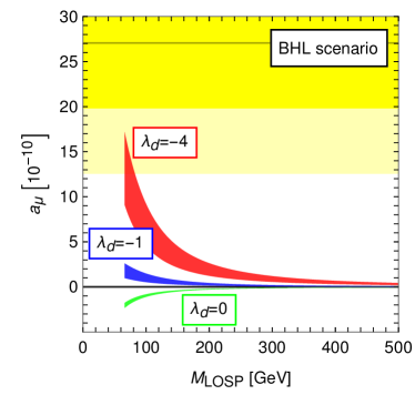
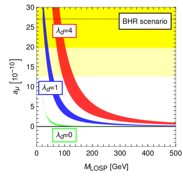
Figure 5: $a_{\mu}$ in the BHL and BHR scenarios. In each plot, the colours of the bands correspond to different values of $\lambda_{d}$ as indicated; the width of each band corresponds to a variation of the slepton masses by a factor $1.5$: the borders of each band correspond to the choices $m_{\tilde{l},\tilde{e},{22}}=m_{\text{SUSY}}$ or $=1.5m_{\text{SUSY}}$. The dark and light yellow horizontal bands correspond to the $1\sigma$ and $2\sigma$ bands given by Eq. (43).

  

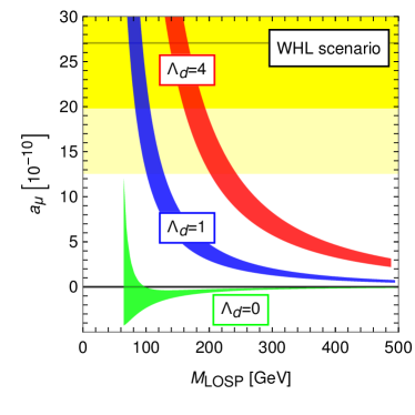
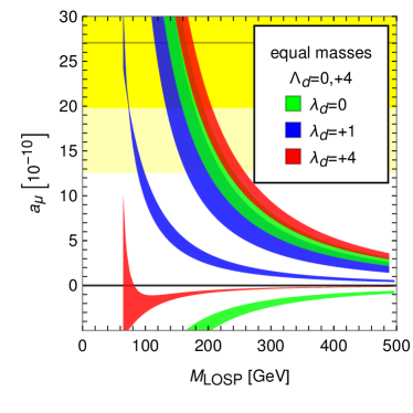
Figure 6: As Fig. 5, but for the WHL and equal-mass scenarios; in the left plot, the values of $\Lambda_{d}$ are indicated; in the right plot, the topmost three bands correspond to $\Lambda_{d}=+4$, the lower three bands to $\Lambda_{d}=0$.

Figure 5 and Figure 6 (left) show the results for $a_{\mu}$ in the BHL, BHR, WHL scenarios. The results are shown as functions of the “lightest observable SUSY mass” $m_{\text{LOSP}}$, defined as the minimum of the electrically charged SUSY particle masses. The $\lambda_{d},\Lambda_{d}$ parameters are varied, and their signs are chosen such that $a_{\mu}$ is positive.

As expected from the result of the mass-insertion diagrams above, $a_{\mu}$ is essentially proportional to $\lambda_{d}$ or $\Lambda_{d}$, as appropriate. And as expected the results are significantly smaller than the corresponding MSSM results for large $\tan\beta$ due to the absence of a $\tan\beta$ enhancement. The largest contribution can be obtained from the WHL scenario because of the larger SU(2) gauge coupling. In the blue bands, $\Lambda_{d}=1$ (corresponding to a value similar to the top-Yukawa coupling). Here the current $a_{\mu}$ deviation can be explained for $m_{\text{LOSP}}$ around 100 GeV at the $2\sigma$ level; for $\Lambda_{d}=4$ (red bands), the current deviation can be explained up to $m_{\text{LOSP}}$ around 200 GeV. We do not consider larger values of $\Lambda_{d}$ because of perturbativity.

The BHR contribution is slightly smaller than the WHL contribution, and the BHL contribution is again smaller, because of the smaller hypercharge. In the BHR case $a_{\mu}$ is just large enough for a $1\sigma$ explanation of the current deviation if $m_{\text{LOSP}}$ is around 100 GeV and $\lambda_{d}=4$. In the BHL case this is impossible, and $a_{\mu}$ reaches at most around $10\times 10^{-10}$.

The remaining contribution for vanishing $\lambda$’s, $\lambda_{d}=\Lambda_{d}=0$ is tiny; its magnitude is always below $2\times 10^{-10}$ as long as $m_{\text{LOSP}}>100$ GeV.

Figure 6(right) shows $a_{\mu}$ in the equal-mass scenario. We see that the value of $\Lambda_{d}$ is far more important than the value of $\lambda_{d}$. The maximum is reached if both $\Lambda_{d}$ and $\lambda_{d}$ are large, i.e. if the WHL and BHR contributions add up constructively. For $\Lambda_{d}=\lambda_{d}=4$, the current $a_{\mu}$ deviation can be explained at the $1\sigma$ ($2\sigma$) level for $m_{\text{LOSP}}$ slightly higher than 200 GeV (250 GeV).

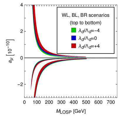
Figure 7: $a_{\mu}$ in the WL (top three bands), BL (middle three bands), BR (bottom three bands) scenarios. The three bands correspond to three different choices of $\lambda_{d}$, $\Lambda_{d}$, as appropriate; the width of the bands is defined as in Fig. 5.

Figure 7 shows $a_{\mu}$ in the BL, BR, WL scenarios. In these scenarios no enhanced chirality-flips are possible, and the $\lambda_{d},\Lambda_{d}$-parameters play a minor role via the chargino/neutralino mass matrices. Overall the values of $a_{\mu}$ are tiny and almost entirely negligible.

The width of the bands in Figs. 5,6,7 corresponds to the variation of the slepton masses by a factor $1.5$, see the definition of the scenarios in Eq. (104). In all cases, the maximum results for $a_{\mu}$ are obtained for the case of fully degenerate spectra, while mass splittings tend to decrease $a_{\mu}$. As discussed in sec. 4.1, some parameter points with certain non-vanishing mass splittings might be excluded by LHC data; thus we see here that these exclusions cannot not affect the upper borders of the bands and the overall maximum contributions for $a_{\mu}$. Similar comments will apply to the plots in the forthcoming subsections.

4.3 Analysis of $\mu\to e\gamma$ in the MRSSM

Now we turn to $\mu\to e\gamma$ in the MRSSM. Clearly there is a strong similarity between $\mu\to e\gamma$ and $a_{\mu}$. Both are given by dipole amplitudes; the difference is the existence of a flavour transition in $\mu\to e\gamma$. The dependence on the LFV parameters $\delta_{12}^{{\text{L}},{\text{R}}}$ is very simple. Neglecting terms suppressed by the electron mass, the amplitude $A_{2}^{\bar{e}\mu{\text{L}}}$ is proportional to $\delta_{12}^{\text{L}}$ and $A_{2}^{\bar{e}\mu{\text{R}}}$ is proportional to $\delta_{12}^{\text{R}}$ to a very good approximation. Hence we may write $A_{2}^{\bar{e}\mu{\text{L}}}\approx A_{2\text{ red}}^{\bar{e}\mu{\text{L}}}\times\delta_{12}^{\text{L}}$ with a “reduced” amplitude $A_{2\text{ red}}^{\bar{e}\mu{\text{L}}}$, and similarly for the right-handed amplitude. Schematically we then have

$$B_{\mu\to e\gamma}\propto|A_{2\text{ red}}^{\bar{e}\mu{\text{L}}}|^{2}\times|\delta_{12}^{\text{L}}|^{2}+|A_{2\text{ red}}^{\bar{e}\mu{\text{R}}}|^{2}\times|\delta_{12}^{\text{R}}|^{2}\,,$$ (119)

while $a_{\mu}$ can be expressed as

$$a_{\mu}\propto A_{2}^{\bar{\mu}\mu{\text{L}}}+A_{2}^{\bar{\mu}\mu{\text{R}}}\,,$$ (120)

with an obvious extension of the notation introduced in Sec. 3. These two equations specify the dependence on the $\delta$’s and the relation between the two observables.

As a result, the analysis of the dependence on SUSY masses and $\Lambda_{d}$, $\lambda_{d}$ of the previous subsection on $a_{\mu}$ carries over to $\mu\to e\gamma$, and there is a strong correlation with $a_{\mu}$.

Figure 8(left) shows this correlation and displays $\mu\to e\gamma$ as a function of $a_{\mu}$ for the three scenarios BHL, BHR, WHL (see Eq. (104)) and for different choices for $\Lambda_{d}$, $\lambda_{d}$ as indicated. In the BHL and WHL scenarios only $\delta_{12}^{\text{L}}$ is nonzero while $\delta_{12}^{\text{R}}=0$, see Eq. (104). In the BHR scenario only $\delta_{12}^{\text{R}}$ is nonzero and $\delta_{12}^{\text{L}}=0$. We see that in each scenario, $\mu\to e\gamma$ is essentially proportional to $|a_{\mu}|^{2}$ as expected. The proportionality coefficient depends on the case — for fixed $a_{\mu}$, the BHL and BHR scenarios give slightly larger $\mu\to e\gamma$. In each scenario the correlation furthermore depends on $\Lambda_{d}$ or $\lambda_{d}$ (as appropriate), and on the mass ratio between the smuon and the other light masses. The borders of the regions are defined by taking the respective smuon mass as either $m_{\text{SUSY}}$ or $1.5\times m_{\text{SUSY}}$ in Eq. (104).

  

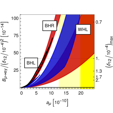
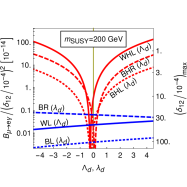
Figure 8: Left: Correlation between $a_{\mu}$ and $B_{\mu\to e\gamma}$ in the WHL, BHL, BHR scenarios, for $|\lambda_{d}|,|\Lambda_{d}|=1$ (blue) and $=4$ (red). The signs for the $\Lambda_{d},\lambda_{d}$ are chosen as in Figs. 5, 6(left). The axis on the left shows $B_{\mu\to e\gamma}$ for the fixed value of the appropriate $\delta_{12}=10^{-4}$, the axis on the right shows the maximum $\delta_{12}$ allowed by the MEG limit (47), see text for details. The very small blue region corresponds to BHR ($\lambda_{d}=1$); the black edgy contour corresponds to the BHL region with $|\lambda_{d}|=4$; the BHL region with $|\lambda_{d}|=1$ is invisibly small. Right: Detailed dependence of $B_{\mu\to e\gamma}$ on $\Lambda_{d},\lambda_{d}$ in the WHL, BHL, BHR, WL, BL, BR scenarios. In each scenario only one of the $\Lambda_{d},\lambda_{d}$ and only one of the $\delta_{12}^{{\text{L}}}$, $\delta_{12}^{{\text{R}}}$ is nonzero, see text for details. The axes are as for the left plot.

The result for $\mu\to e\gamma$ can be interpreted in two ways, as indicated by the axis labels on the left and right border of the plot. On the left border we indicate the value of $B_{\mu\to e\gamma}$ for the fixed value of the appropriate $\delta_{12}=10^{-4}$. In all scenarios $\mu\to e\gamma$ then varies in the range up to around $10^{-12}$ in the considered range for $a_{\mu}$. On the other hand, in view of Eq. (119) this allows to obtain $B_{\mu\to e\gamma}$ for any other value of the appropriate $\delta_{12}$. Conversely, it also allows to determine the value of the $\delta_{12}$, for which $B_{\mu\to e\gamma}$ is equal to the MEG limit (47). This is shown on the axis on the right border of the plot. This axis corresponds to the maximum $\delta_{12}$’s allowed for the corresponding points in the plot. We see that they are in the range $(0.5\ldots 2)\times 10^{-4}$ if $a_{\mu}$ is in the $2\sigma$-band around its experimental value.

In the plot we do not show the scenarios BL, BR, WL and $\Lambda_{d},\lambda_{d}=0$ since these cases lead to tiny $a_{\mu}$. However the correlation would be of a similar kind. We also do not show the equal-mass scenario since there destructive interference between different amplitudes can happen, as will be studied below. Overall, Fig. 8(left) is very similar to the corresponding MSSM result shown in Ref. Kersten:2014xaa .

Figure 8(right) shows the more detailed dependence of $\mu\to e\gamma$ in six scenarios, including the BL, BR, WL scenarios. In each case, only one of the two $\delta_{12}$’s is nonzero, as appropriate, see (104): for BHR and BR, only $\delta_{12}^{{\text{R}}}$ is nonzero, in the other cases only $\delta_{12}^{{\text{L}}}$. The plot then shows $B_{\mu\to e\gamma}$ as a function of either $\Lambda_{d}$ (for WHL and WL) or $\lambda_{d}$ (all other cases). The axis on the right border of the plot shows the respective maximum allowed value of $\delta_{12}$ for the respective point in the plot, computed as for Fig. 8(left). All results in Fig. 8(right) are shown for the fixed value of $m_{\text{SUSY}}=200$ GeV. The behaviour for other values of $m_{\text{SUSY}}$ would be very similar; the branching ratio simply scales as $1/m_{\text{SUSY}}^{4}$, and the maximum $\delta_{12}$’s scale as $m_{\text{SUSY}}^{2}$.

The results shown in the plot are similar to the corresponding results for $a_{\mu}$: The scenarios without Higgsinos WL, BL, BR give very small contributions, which depend on $\Lambda_{d},\lambda_{d}$ only in a minor way via the chargino/neutralino masses. The branching ratio reaches the MEG limit in these scenarios for values of the $\delta_{12}$’s around $(30\ldots 100)\times 10^{-4}$. Due to the scaling with $m_{\text{SUSY}}^{2}$, this equivalently implies that e.g. values of $\delta_{12}$ around $10\%$ are allowed if $m_{\text{SUSY}}$ is in the few TeV range.

The contributions in the scenarios with light Higgsino are significantly enhanced by large $\Lambda_{d}$ and $\lambda_{d}$; the amplitudes are enhanced linearly, while the branching ratios are enhanced quadratically. Like for $a_{\mu}$, the contributions can be largest in the WHL scenario, followed by the BHR and BHL scenarios. For $\Lambda_{d}$, $\lambda_{d}$ bigger than around unity, the contributions in these scenarios reach the MEG limit for around $\delta_{12}\sim 10^{-4}\ldots 10^{-3}$.

The scenarios with light Higgsino show an interesting behaviour at small $\Lambda_{d},\lambda_{d}$. If $\Lambda_{d},\lambda_{d}=0$, only contributions governed by gauge couplings remain, and the branching ratio becomes similarly small as in the WL, BL, BR scenarios. For certain small but nonzero values of $\Lambda_{d},\lambda_{d}$ the amplitudes pass through zero and the branching ratio vanishes.

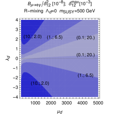
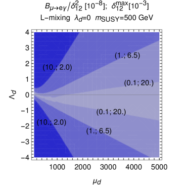
(a)    (b)

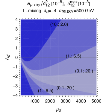
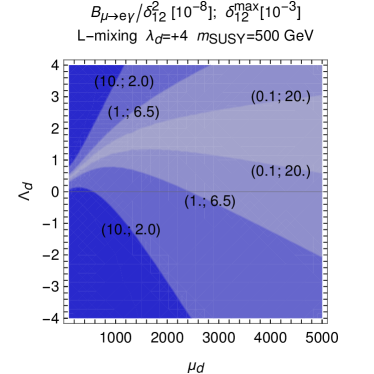
(c)    (d)

Figure 9: $\mu\to e\gamma$ in the equal-mass scenario, with $\mu_{d}$ kept as a free parameter. In plot (a) only $\delta_{12}^{{\text{R}}}$ is nonzero, while $\delta_{12}^{{\text{L}}}=0$; opposite in plots (b,c,d). The values of $\Lambda_{d},\lambda_{d}$ are indicated in the plots. The contours correspond on the one hand to $B_{\mu\to e\gamma}/(\delta_{12})^{2}$ and on the other hand to the maximum $\delta_{12}$ allowed by the MEG limit. See Eqs. (121,122) for an approximation of the behaviour.

Figure 9 shows the interference between contributions with and without Higgsinos. We begin with describing plot 9(a). Here only right-handed mixing $\delta_{12}^{{\text{R}}}$ is nonzero, while $\delta_{12}^{{\text{L}}}=0$. We consider the equal-mass scenario of Eq. (104) with $m_{\text{SUSY}}=500$ GeV, with the exception of the Higgsino mass $\mu_{d}$, which is kept as a variable. The contour plot then shows $\mu\to e\gamma$ as a function of $\mu_{d}$ and $\lambda_{d}$ for $\Lambda_{d}=0$. Again, the contours are interpreted in two ways. On the one hand they indicate $B_{\mu\to e\gamma}/(\delta_{12}^{{\text{R}}})^{2}$, on the other hand they allow to read off the maximum $\delta_{12}^{{\text{R}}}$ allowed by the MEG limit.

The behaviour of Fig. 9(a) arises from interference of BHR-type and BR-type contributions. For small $\mu_{d}$ and large $\lambda_{d}$, the BHR-type contributions dominate and show the expected $\lambda_{d}$-enhancement. The corresponding parts of the amplitude behave as $\lambda_{d}/\mu_{d}$. The BR-type contributions are approximately independent of $\lambda_{d}$ and $\mu_{d}$. In fact, the behaviour in plot (a) can be well approximated by the simple fit

$$B_{\mu\to e\gamma} \approx\left(\frac{1500\text{ GeV}}{\mu_{d}}\lambda_{d}-0.4\right)^{2}\times{10^{-8}}\left(\delta_{12}^{{\text{R}}}\right)^{2}\,,$$ (121)

at large $\mu_{d}$, exhibiting the two types of contributions. This also allows to understand the triangular region with very small $B_{\mu\to e\gamma}$ in which the $\lambda_{d}$-enhanced terms are cancelled by the BR-type contributions.

Figures 9(b,c,d) are similar but for nonzero left-handed mixing $\delta_{12}^{{\text{L}}}$ and as a function of $\Lambda_{d}$ for different choices of $\lambda_{d}$. In plot (b) the behaviour is similar to the one in plot (a) but it arises essentially from a combination of WHL- and WL-type contributions; in plots (c,d) also the BHL- and BL-type contributions matter and shift the contours according to the choice of $\lambda_{d}$. The behaviour in these plots at large $\mu_{d}$ can be approximated by

$$B_{\mu\to e\gamma} \approx\left(\frac{1200\text{ GeV}}{\mu_{d}}\left(\Lambda_{d}-\frac{\lambda_{d}}{2}\right)+0.11\right)^{2}\times 10^{-8}\left(\delta_{12}^{{\text{L}}}\right)^{2}\,.$$ (122)

4.4 Analysis of $\mu\to e$ conversion in the MRSSM

The next observable we investigate is $\mu\to e$ conversion. This observable has a much more complicated parameter dependence than the previous observables. It depends on four types of form factors $A_{1}$, $A_{2}$, $A_{Z}$, $A_{\text{box}}$, corresponding to the charge radius, the dipole, the $Z$-penguin and box diagrams. The previous observables only depended on dipole form factors.

The behaviour of the dipole form factor has been discussed in the the previous subsections in detail, so here we focus particularly on the additional parameter dependence arising from the new form factors. Not all parameters lead to a nontrivial dependence. All form factors are linear in the generation mixing parameters $\delta_{12}^{{\text{L}},{\text{R}}}$ to a very good approximation. Therefore we fix the $\delta_{12}$’s to the standard values of Sec. 4.1, i.e. to $10^{-4}$ or to zero, depending on the scenario. Furthermore, all form factors are proportional to $1/m_{\text{SUSY}}^{2}$, where $m_{\text{SUSY}}$ is a representative mass scale. Hence we also fix the overall mass scale to $m_{\text{SUSY}}=500$ GeV for our discussion.

A very useful quantity to study is the ratio between the two branching ratios for $\mu\to e$ and $\mu\to e\gamma$,

$$R(\text{Al})\equiv\frac{{B_{\mu\text{Al}\to e\text{Al}}}}{B_{\mu\to e\gamma}}\,.$$ (123)

In this ratio, the generic dependence on the $\delta$’s and the masses drops out. Knowledge of $R(\text{Al})$ also tells us the maximum possible $\mu\to e$ conversion rate given the MEG limit on $\mu\to e\gamma$ for any given parameter scenario. Interestingly, if $\mu\to e$ is dominated by the dipole form factors, then all model dependence, i.e. the full form factors $A_{2}$ drop out in the ratio $R(\text{Al})$ and there is a perfect correlation. The correlation only depends on the element used in the experiment; for Aluminum the prediction for dipole dominance is Kitano:2002mt

$$R^{\text{only dip.}}(\text{Al}) =0.0026\,.$$ (124)

Deviations of the actual result for $R(\text{Al})$ from this prediction then highlight the impact of the additional form factors $A_{1}$, $A_{Z}$, $A_{\text{box}}$.

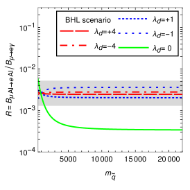
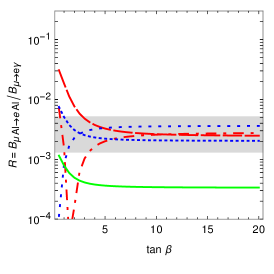
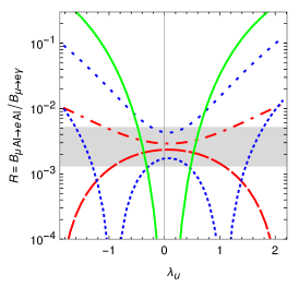
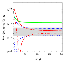
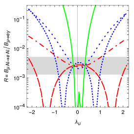
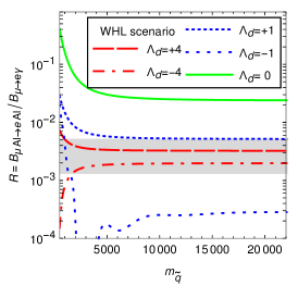
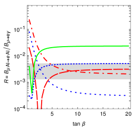
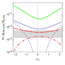
Figure 10: The ratio $R(\text{Al})$ of the $\mu\to e$ and $\mu\to e\gamma$ branching ratios as function of the squark mass, $\tan\beta$, and of $\lambda_{u}$ or $\Lambda_{u}$, as appropriate. The plots in the first, second, and third rows correspond to the BHL, BHR, WHL scenarios, respectively; the legends correspond to all plots in each row. In each plot all parameters are fixed to the standard values for each scenario with $m_{\text{SUSY}}=500$ GeV except in the $\lambda_{u}$, $\Lambda_{u}$ plots, where $\mu_{u}=m_{\text{SUSY}}$. The gray band indicates the expectation corresponding to dipole dominance, Eq. (124), allowing a fluctuation by a factor 2 up or down.

Before describing detailed plots we provide an overview of the behaviour of the four form factors.

• $A_{1}$: $A_{1}$ is dominated by diagrams with exchange of gaugino-like charginos/neutralinos. There is only a mild parameter dependence and no significant enhancement by light or heavy Higgsino masses, by large or small $\lambda$’s, by large or small $\tan\beta$. $A_{1}$ is largest in scenarios with light wino and slightly smaller if only the bino mass is light.

• $A_{2}$: As discussed for $a_{\mu}$ and $\mu\to e\gamma$, the dipole form factor is essentially linearly enhanced by $\lambda_{d}$, $\Lambda_{d}$ if $\mu_{d}$ is light. The remaining terms are small and of a similar size as $A_{1}$. Hence if the dipole is not enhanced, there can be significant constructive or destructive interference between $A_{1}$ and $A_{2}$ within $\mu\to e$ conversion.

• $A_{Z}$: The $Z$-penguin contributions are smaller than the $A_{1}$ and $A_{2}$ contributions in a large parameter region. The Feynman diagrammatic reason is that the $Z$ boson only couples to Higgsino-like charginos/neutralinos (this is obvious from the neutralino–$Z$ Feynman rule; for the charginos there is a cancellation between diagram types 1,2,3,4 in Fig. 2, see also the MSSM case Hisano:1995cp ). On the other hand, for the same reason the $Z$-penguin can be strongly enhanced proportional to

  $$\propto v_{d}^{2}\lambda_{d}^{2}\,, \propto v_{d}^{2}\Lambda_{d}^{2}\,,$$ (125a)

  $$\propto v_{u}^{2}\lambda_{u}^{2}\,, \propto v_{u}^{2}\Lambda_{u}^{2}\,,$$ (125b)

  corresponding to two insertions of gaugino–Higgsino mixing terms. The enhancements proportional to $v_{d}^{2}$ become important for small $\tan\beta$, leading to a $1/\tan^{2}\beta$ enhancement. The enhancements proportional to $v_{u}^{2}$ become important if the up-type Higgsino $\mu_{u}$ is light. A similar but smaller enhancement governed by gauge couplings instead of $\lambda$’s has been discussed in Ref. Fok:2010vk .

• $A_{\text{box}}$: The box diagrams are negligible for large squark masses; for small $m_{\tilde{q}}$ they reach similar values as $A_{1}$ and have a similarly mild dependence on all other parameters.

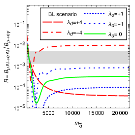
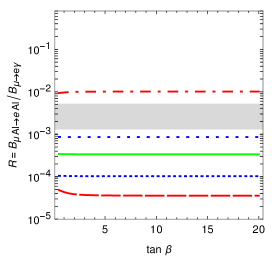
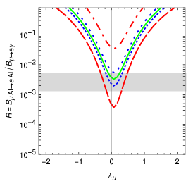
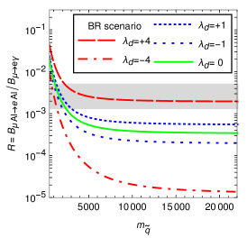
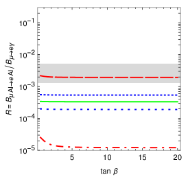
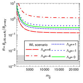
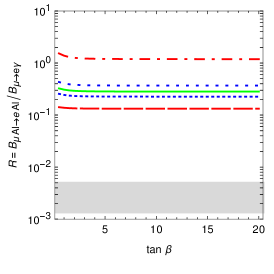
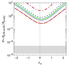
Figure 11: As Fig. 10, but for the scenarios BL, BR, WL without light $\mu_{d}$.

Figures 10 and 11 show the behaviour of the ratio of branching ratios $R(\text{Al})$ as a function of all relevant parameters in the six scenarios BHL, BHR, WHL, BL, BR, WL. Each row in the Figures corresponds to one of the scenarios. For each scenario, $m_{\text{SUSY}}=500$ GeV fixed and $\lambda_{d}$ or $\Lambda_{d}$ is set to the five values $\pm 4$, $\pm 1$, 0. The first plot in each row shows $R(\text{Al})$ as a function of the squark mass $m_{\tilde{q}}$, the second plot as a function of $\tan\beta$, and the third plot as a function of $\lambda_{u}$ or $\Lambda_{u}$ (as appropriate) while $\mu_{u}=m_{\text{SUSY}}$. All other parameters are set to the standard values explained in Sec. 4.1. The gray band indicates the expectation corresponding to dipole dominance, Eq. (124), allowing an up or down fluctuation by a factor 2.

The plots allow to easily read off under which conditions dipole dominance holds and under which conditions $\mu\to e$ can be enhanced relative to $\mu\to e\gamma$. The cases with enhanced $\mu\to e$ are very interesting in view of the forthcoming COMET and Mu2e experiments since they allow signals in those experiments without violating the MEG limit on $\mu\to e\gamma$.

For the discussion we first focus on the regions of large $m_{\tilde{q}}$ in the squark mass plots in the first column and large $\tan\beta$ in the $\tan\beta$ plots in the second column. These regions show the “baseline behaviour” resulting only from the form factors $A_{1}$ and $A_{2}$, while the $Z$-penguin and box diagrams are negligible. The results for large $|\lambda_{d}|$, $|\Lambda_{d}|$ in the BHL, BHR, WHL scenarios are in the gray region: this corresponds to the expected dipole dominance for light Higgsino mass $\mu_{d}$ and large $|\lambda_{d}|$, $|\Lambda_{d}|$ resulting from the mass insertion diagrams discussed in Sec. 4.2.

If $\lambda_{d},\Lambda_{d}=0$ in the BHL, BHR, WHL scenarios, the form factors $A_{1}$ and $A_{2}$ are of a similar size. The same is true in the BL, BR, WL scenarios, independently of $\lambda_{d}$, $\Lambda_{d}$. Hence in all these cases we get strong deviations from dipole dominance $R^{\text{only dip.}}(\text{Al})$. The actual ratio ranges from $R(\text{Al})\sim 10^{-5}$ in the BR scenario (due to an accidental cancellation between $A_{1}$ and $A_{2}$ which happens around $\lambda_{d}\approx-4$) up to $R(\text{Al})\sim 1$ in the WL scenario (where $A_{1}$ is a few times larger than $A_{2}$).

Next we focus on the dependence on $m_{\tilde{q}}$, which arises only from the box diagrams. For large squark masses they are negligible and we obtain the baseline behaviour discussed before; for smaller squark masses below around $5\times m_{\text{SUSY}}$ they become relevant. Of course, their impact is particularly pronounced in cases where the dipole $A_{2}$ is small, i.e. for small $\lambda_{d},\Lambda_{d}$ and/or in the BL, BR, WL scenarios. In these cases the box diagrams can increase $\mu\to e$ by a factor of a few.

Finally we describe the influence of the $Z$-penguin contributions. They are enhanced by two powers of the gaugino–Higgsino mixing, see Eq. (125). The enhancements governed by $v_{d}^{2}$ and $\lambda_{d}^{2},\Lambda_{d}^{2}$ are visible in the $\tan\beta$ plots at small $\tan\beta$, where these terms become large. For $\tan\beta\leq 5$, this effect can lead to dramatic enhancements in the scenarios with light Higgsino mass $\mu_{d}$.

The enhancements governed by $v_{u}^{2}$ and $\lambda_{u}^{2},\Lambda_{u}^{2}$ can be seen in the $\lambda_{u}$, $\Lambda_{u}$ plots in the third column. For small $\lambda_{u}$, $\Lambda_{u}$, the results are similar to the baseline behaviour discussed above (the slight differences are due to $\mu_{u}=m_{\text{SUSY}}$ instead of $\mu_{u}\gg m_{\text{SUSY}}$). For larger values of $\lambda_{u}$, $\Lambda_{u}$ the $Z$-penguin dominates, leading to very strong enhancements as well as to zeroes in $\mu\to e$ due to cancellations between the different form factors.

The largest overall values of the ratio of branching ratios can reach more than $R(\text{Al})>10$ in the scenarios with small dipoles (i.e. for small $\lambda_{d},\Lambda_{d}$ and/or the scenarios BL, BR, WL with heavy $\mu_{d}$). In scenarios with large dipole, e.g. in the WHL scenario with $\Lambda_{d}=1$, $R(\text{Al})$ can still be 10 times larger than the value $R^{\text{only dip.}}(\text{Al})$.

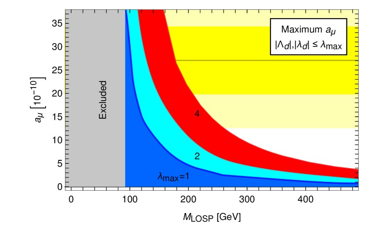
Figure 12: Maximum possible results for $a_{\mu}$ in the MRSSM obtained from a parameter scan applying the constraints of Sec. 4.1 and maximum values for $\Lambda_{d}$, $\lambda_{d}$ as indicated in the plot. The dark and light yellow horizontal bands correspond to the $1\sigma$ and $2\sigma$ bands given by Eq. (43). The vertical band corresponds to the exclusion limit (105).

4.5 Summary plots based on scans

The previous subsections have analyzed the detailed parameter dependences of all three observables $a_{\mu}$, $\mu\to e\gamma$ and $\mu\to e$ conversion in the MRSSM. In the present subsection we will show several plots based on parameter scans. These plots summarize the generic behaviour and show maximum possible results and the correlations between the observables.

Figure 12 shows the maximum possible results for $a_{\mu}$ in the MRSSM, as a function of the LOSP mass, i.e. the lightest electrically charged SUSY particle mass. It is based on a scan in parameter space where the ratios between the masses are varied and various upper limits on $\Lambda_{d},\lambda_{d}$ are imposed. As expected from section 4.2 and Fig. 6 the maximum $a_{\mu}$ is obtained in scenarios where the WHL- and BHR-like contributions add up constructively and the corresponding masses are all similar. Again the plot shows that very small masses are required to explain the current $a_{\mu}$ deviation. For $|\Lambda_{d}|<4$, a $1\sigma$ explanation requires $m_{\text{LOSP}}<200$ GeV, and for $|\Lambda_{d}|<2$, it requires $m_{\text{LOSP}}<150$ GeV.

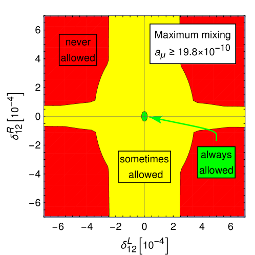
Figure 13: Scan over parameter choices for which $a_{\mu}$ agrees with the deviation (43), displaying regions for $\delta^{{\text{L}}}_{12}$ and $\delta^{{\text{R}}}_{12}$ allowed by the MEG limit on $\mu\to e\gamma$ (47). The small, inner green region is allowed by all parameter choices which explain $a_{\mu}$, the cross-shaped large yellow region is allowed by some parameter choices, and the outer red region is not allowed by any parameter choice.

Figure 13 focuses on the correlation between $a_{\mu}$ and $\mu\to e\gamma$. It derives limits on the flavour-violating parameters $\delta^{{\text{L}},{\text{R}}}_{12}$, valid under the condition that the $a_{\mu}$ deviation is fully explained by the MRSSM. The logic behind this plot is as follows. For each parameter choice with a certain value of $a_{\mu}$, the prediction for $\mu\to e\gamma$ is essentially fixed, since both observables are governed by dipole form factors, see Fig. 8. The only remaining free parameters are the $\delta^{{\text{L}},{\text{R}}}_{12}$, which enter as in Eq. (119). As a result, for each parameter choice which explains the $a_{\mu}$ deviation, there is a certain ellipse-shaped region in the $\delta^{{\text{L}}}_{12}$–$\delta^{{\text{R}}}_{12}$-space allowed by the MEG limit on $\mu\to e\gamma$.

Fig. 13 shows the results of a scan over all parameter choices for which the current $a_{\mu}$ deviation is explained, and for which the parameter constraints of Sec. 4.1 are met. The values of the $\delta$’s in the small green inner contour are allowed by all parameter choices (i.e. $\mu\to e\gamma$ is always below the MEG limit). This inner contour arises from the intersection of all ellipses and has itself approximately the shape of an ellipse. On the other hand, the values of the $\delta$’s in the large cross-like yellow region are allowed by some parameter choices and forbidden by others; this region corresponds to the union of all ellipses. The cross-like shape arises because for certain parameter choices the ellipses degenerate to large rectangles: For the WHL-like case shown in Fig. 8, $\mu\to e\gamma$ only depends on $\delta^{{\text{L}}}_{12}$ and hence there is an upper limit on $\delta^{{\text{L}}}_{12}$ but $\delta^{{\text{R}}}_{12}$ can be arbitrarily large; similarly BHR-like parameter choices lead to unconstrained $\delta^{{\text{L}}}_{12}$. Numerically, values of the $\delta$’s below around $10^{-5}$ are always allowed. On the other hand, choices where both $\delta_{12}$’s are significantly above around $10^{-4}$ are always forbidden.

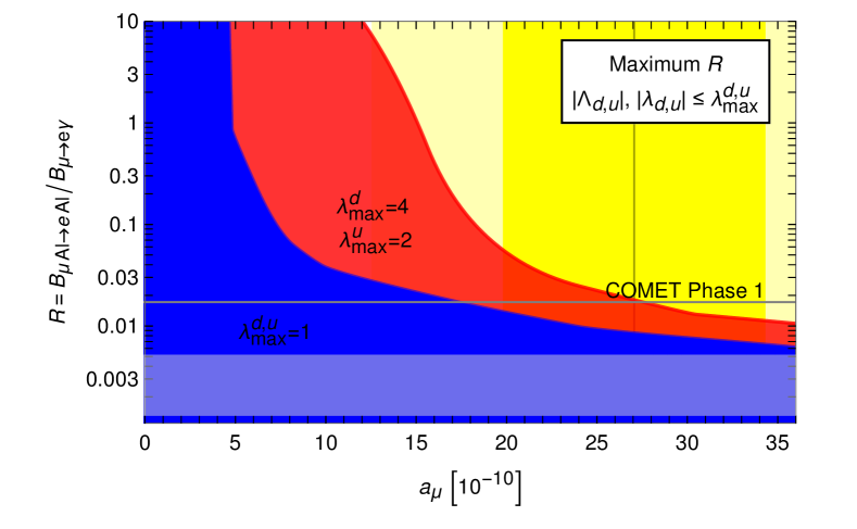
Figure 14: The correlation between $\mu\to e$ conversion and $\mu\to e\gamma$, as a function of $a_{\mu}$; equivalently, the maximum value for $\mu\to e$ conversion for a given value of $\mu\to e\gamma$. The possible ranges have been obtained from a parameter scan respecting the constraints of Sec. 4.1. In particular, in the outer red region, the $\lambda$’s take the maximum values allowed in Sec. 4.1; in the blue inner region the $\lambda$’s are constrained to be less than unity. The vertical yellow band is defined as in Fig. 5; the horizontal light gray band indicates the expectation corresponding to dipole dominance as in Fig. 10. The thin horizontal line indicates the minimum value of $R(\text{Al})$ for which COMET Phase 1 is sensitive to $\mu\to e$ conversion, given the current MEG limit on $\mu\to e\gamma$.

Figure 14 focuses on the correlation of all three observables $a_{\mu}$, $\mu\to e\gamma$ and $\mu\to e$ conversion. It is based on the following expectation. If $a_{\mu}$ is large, the dipole form factor must be large, and in dipole-dominated cases $\mu\to e\gamma$ and $\mu\to e$ are strongly correlated, see Eq. (124). If $a_{\mu}$ is small, the dipole form factor can be small and $\mu\to e\gamma$ and $\mu\to e$ become uncorrelated. Therefore Fig. 14 shows the ratio $R(\text{Al})={B_{\mu\text{Al}\to e\text{Al}}}/{B_{\mu\to e\gamma}}$ as a function of $a_{\mu}$ in a parameter scan fulfilling the constraints of Sec. 4.1. The scan is further constrained by $\delta^{{\text{L}}}_{12}=\delta^{{\text{R}}}_{12}$.

The result has the expected behaviour. If $a_{\mu}\gtrsim 30\times 10^{-10}$, the ratio $R(\text{Al})$ is within the expectation of dipole dominance up to a factor 5, and even up to a factor 2 if all $\lambda_{i}$, $\Lambda_{i}$ are constrained to be below unity. Combining this upper limit on $R(\text{Al})$ with the MEG limit on $\mu\to e\gamma$ shows that in this parameter region the $\mu\to e$ conversion rate is below the reach of COMET Phase 1. In the plot, this can be seen with the help of the thin horizontal line, which corresponds to $R(\text{Al})=0.017$, the ratio of the COMET Phase 1 sensitivity and the MEG limit (47).

If $a_{\mu}>12\times 10^{-10}$, just within the $2\sigma$ region around the observed deviation, the ratio $R(\text{Al})$ can be 10 times larger even for moderate $\lambda_{i}$, $\Lambda_{i}$. This is interesting in view of the forthcoming COMET Phase 1 measurement of $\mu\to e$ conversion: a positive signal at COMET Phase 1 is possible while $\mu\to e\gamma$ remains below the current MEG limit.

For lower $a_{\mu}$ and/or larger values of the $\lambda_{i}$ and $\Lambda_{i}$, $R(\text{Al})$ can be even larger. The parameter choices which maximize $R(\text{Al})$ are choices where $\Lambda_{u}$ and $\lambda_{u}$ take values at the border of the allowed region and where all masses except the Higgsino masses are very similar. In such parameter regions the MRSSM prediction for $\mu\to e$ conversion can be easily in reach of COMET Phase 1 even if $\mu\to e\gamma$ is orders of magnitude below the current MEG limit.

As mentioned above, Fig. 14 uses the constraint $\delta^{{\text{L}}}_{12}=\delta^{{\text{R}}}_{12}$ (the actual value drops out in the ratio $R(\text{Al})$ and is not important). If this constraint is dropped and $\delta^{{\text{L}}}_{12}=0$ or $\delta^{{\text{R}}}_{12}=0$ are allowed, the ratio $R(\text{Al})$ becomes unconstrained. E.g. we could choose a WHL-like mass pattern with large $a_{\mu}$ and tune the masses and $\lambda_{d}$ such that the right-handed dipole amplitude vanishes. If we then set $\delta^{{\text{L}}}_{12}=0$ but $\delta^{{\text{R}}}_{12}\neq 0$, all flavour-violating dipole amplitudes vanish and $\mu\to e\gamma$ is impossible, while $\mu\to e$ conversion is still possible due to the other form factors. Accordingly $R(\text{Al})$ can be arbitrarily large independently of $a_{\mu}$ if one of the $\delta$’s is allowed to vanish.

5 Conclusions

The MRSSM provides an attractive alternative realization of SUSY with promising phenomenological properties. In the present paper we have considered the MRSSM predictions for $a_{\mu}$ and the lepton-flavour violating observables $\mu\to e\gamma$ and $\mu\to e$. We presented analytic one-loop results, useful compact approximations and a detailed numerical analysis.

A striking difference to the familiar MSSM case is the absence of $\tan\beta$ enhancements in all dipole amplitudes. The reason is that the $\tan\beta$ enhancement in the MSSM originates from insertions of the MSSM $\mu$-parameter and Majorana gaugino masses. Both are forbidden in the MRSSM by R-symmetry. The absence of $\tan\beta$ enhancements alters the phenomenology significantly.

In spite of this we have found that dipole amplitudes can be enhanced in the MRSSM by MRSSM-specific superpotential parameters $\Lambda_{d}$, $\lambda_{d}$. The mechanism is similar to the $\tan\beta$ enhancements in the MSSM but its numerical impact is restricted by constraints on the superpotential parameters from electroweak precision observables and perturbativity.

The analysis of $a_{\mu}$ has shown that it is very hard to explain the currently observed deviation in the MRSSM. An explanation is possible only in particular corners of the MRSSM parameter space: several SUSY masses, among them at least one smuon, one gaugino and one Higgsino, should be around 200 GeV or below and the values of $\Lambda_{d}$ and/or $\lambda_{d}$ should be at least as large as the top Yukawa coupling, preferably larger. Such parameter choices are viable since compressed light spectra are not excluded by LHC data.

The required large values of $\Lambda_{d}$, $\lambda_{d}$ are intriguing. Similar large values of $\Lambda_{u}$, $\lambda_{u}$ have been found helpful in explaining the measured value of the Higgs boson mass Diessner:2014ksa ; on the other hand very large values of these parameters are constrained by electroweak precision data and are difficult to reconcile with embedding the MRSSM into an $N=2$ SUSY theory.

The decay $\mu\to e\gamma$ is strongly correlated to $a_{\mu}$ if $a_{\mu}$ is large. As a result we could derive limits on the flavour-violating parameters $\delta^{{\text{L}},{\text{R}}}_{12}$ valid under the assumption that the MRSSM explains the current $a_{\mu}$ deviation. As shown in the traffic-light-like colours of Fig. 13 values for the $\delta$’s below around $10^{-5}$ are generally allowed and higher values can be allowed, depending on the choice of parameters. It is however also of interest to discuss $\mu\to e\gamma$ in scenarios with small $a_{\mu}$ — future $a_{\mu}$ measurements could be closer to the SM prediction or non-MRSSM new physics could explain the deviation. In such scenarios larger SUSY masses and small $\Lambda_{d}$, $\lambda_{d}$ are possible and larger $\delta$’s are allowed. Combining Figures 8(right) and 9 with the known mass scaling allows to conclude that $\delta_{12}$’s around $10\%$ become possible for SUSY masses in the few TeV range.

Our reason to consider particularly $\mu\to e$ conversion as another lepton flavour violating observable was threefold. The forthcoming COMET and Mu2e experiments promise to improve the sensitivity to this process by orders of magnitude; an earlier study in Ref. Fok:2010vk already revealed that this process can provide limits on the MRSSM, and we expected characteristic differences between the MRSSM and MSSM predictions for this process. In the MSSM, the process is typically dominated by dipole amplitudes and strongly correlated with $\mu\to e\gamma$, see Eq. (124).

Indeed we found strong deviations from dipole dominance. There are two main sources for these deviations. If the dipole amplitudes are small, the charge radius form factors become relatively important and can dominate strongly. And even if the dipole amplitudes are large, the $Z$-penguin contributions can also be large — they are enhanced $\propto\Lambda_{i}^{2}v_{i}^{2}$ ($i=u,d$). In the fully general case, where mixing in the left-handed and right-handed slepton sectors is independent, there is no correlation between $\mu\to e$ and $\mu\to e\gamma$. Due to possible cancellations either of these observables could be zero while the other is large.

We have then studied the (non-)correlation for the specific condition $\delta^{{\text{L}}}_{12}=\delta^{{\text{R}}}_{12}$. The result is Fig. 14, which shows the ratio between $\mu\to e$ and $\mu\to e\gamma$ as a function of $a_{\mu}$. It shows that if $a_{\mu}$ is as large as the current deviation, the correlation between $\mu\to e$ and $\mu\to e\gamma$ is rather strong, though not as strong as in case of dipole dominance, Eq. (124). In this case, the current MEG limit on $\mu\to e\gamma$ implies an upper limit on the possible MRSSM prediction to $B_{\mu\text{Al}\to e\text{Al}}$ of a few times $10^{-15}$, just touching the reach of COMET Phase I but well in reach of COMET Phase II and the Mu2e experiment.

On the other hand, if $a_{\mu}$ is not quite as large, the correlation between $\mu\to e$ and $\mu\to e\gamma$ becomes weaker. For $a_{\mu}$ contributions below $20\times 10^{-10}$, Fig. 14 together with the MEG limit allows $B_{\mu\text{Al}\to e\text{Al}}$ well in reach of COMET Phase I. Turning the argument around, if COMET Phase I finds a signal for $\mu\to e$ conversion and if the MRSSM is realized in the scenario of Fig. 14, the MRSSM cannot explain the current $a_{\mu}$ deviation at the $1\sigma$ level.

The present paper has focused on a detailed and comprehensive survey, but we have restricted ourselves to three observables, and all our results have been obtained at leading nonvanishing order. We leave the study of further observables such as $\mu\to eee$ and the inclusion of higher-order corrections such as the ones considered in Refs. Davidson:2016edt ; Davidson:2016utf ; Crivellin:2017rmk for later work.

Appendix A MRSSM Feynman rules

Here we provide the values of the coupling coefficients introduced in section 2.3 and the resulting Feynman rules.

Lepton–sleptons–neutralinos/charginos

Up–quarks–squarks–neutralinos/charginos

Down–quarks–squarks–neutralinos/charginos

$Z$–Neutralinos/charginos

$Z$–fermions/sfermions

References

- (1) Muon g-2 collaboration, Muon (g-2) Technical Design Report, 1501.06858.
- (2) J-PARC muon g-2/EDM collaboration, New approach to the muon g-2 and EDM experiment at J-PARC, J. Phys. Conf. Ser. 295 (2011) 012032.
- (3) J-PARC g-2 collaboration, Measurement of muon g-2 and EDM with an ultra-cold muon beam at J-PARC, Nucl. Phys. Proc. Suppl. 218 (2011) 242.
- (4) MEG collaboration, Search for the lepton flavour violating decay with the full dataset of the MEG experiment, Eur. Phys. J. C76 (2016) 434 [1605.05081].
- (5) A. M. Baldini et al., MEG Upgrade Proposal, 1301.7225.
- (6) MEG collaboration, The MEG experiment result and the MEG II status, Nuovo Cim. C41 (2018) 42.
- (7) A. Blondel et al., Research Proposal for an Experiment to Search for the Decay , 1301.6113.
- (8) SINDRUM II collaboration, A Search for muon to electron conversion in muonic gold, Eur. Phys. J. C47 (2006) 337.
- (9) COMET collaboration, Conceptual design report for experimental search for lepton flavor violating conversion at sensitivity of with a slow-extracted bunched proton beam (comet), .
- (10) COMET collaboration, A search for muon-to-electron conversion at J-PARC: The COMET experiment, PTEP 2013 (2013) 022C01.
- (11) COMET collaboration, COMET Phase-I Technical Design Report, 1812.09018.
- (12) Mu2e collaboration, Mu2e Conceptual Design Report, 1211.7019.
- (13) A. Czarnecki, X. Garcia i Tormo and W. J. Marciano, Muon decay in orbit: spectrum of high-energy electrons, Phys. Rev. D84 (2011) 013006 [1106.4756].
- (14) R. Szafron and A. Czarnecki, High-energy electrons from the muon decay in orbit: radiative corrections, Phys. Lett. B753 (2016) 61 [1505.05237].
- (15) G. M. Pruna, A. Signer and Y. Ulrich, Fully differential NLO predictions for the rare muon decay, Phys. Lett. B765 (2017) 280 [1611.03617].
- (16) G. M. Pruna, A. Signer and Y. Ulrich, Fully differential NLO predictions for the radiative decay of muons and taus, Phys. Lett. B772 (2017) 452 [1705.03782].
- (17) M. Lindner, M. Platscher and F. S. Queiroz, A Call for New Physics : The Muon Anomalous Magnetic Moment and Lepton Flavor Violation, Phys. Rept. 731 (2018) 1 [1610.06587].
- (18) G. D. Kribs, E. Poppitz and N. Weiner, Flavor in supersymmetry with an extended R-symmetry, Phys. Rev. D78 (2008) 055010 [0712.2039].
- (19) P. J. Fox, A. E. Nelson and N. Weiner, Dirac gaugino masses and supersoft supersymmetry breaking, JHEP 08 (2002) 035 [hep-ph/0206096].
- (20) R. Fok and G. D. Kribs, in R-symmetric Supersymmetry, Phys. Rev. D82 (2010) 035010 [1004.0556].
- (21) E. Dudas, M. Goodsell, L. Heurtier and P. Tziveloglou, Flavour models with Dirac and fake gluinos, Nucl. Phys. B884 (2014) 632 [1312.2011].
- (22) K.-S. Sun, J.-B. Chen, X.-Y. Yang and S.-K. Cui, The LFV decays of boson in Minimal R-symmetric Supersymmetric Standard Model, 1901.03800.
- (23) E. Bertuzzo, C. Frugiuele, T. Gregoire and E. Ponton, Dirac gauginos, R symmetry and the 125 GeV Higgs, JHEP 04 (2015) 089 [1402.5432].
- (24) P. Dießner, J. Kalinowski, W. Kotlarski and D. Stöckinger, Higgs boson mass and electroweak observables in the MRSSM, JHEP 12 (2014) 124 [1410.4791].
- (25) P. Diessner, J. Kalinowski, W. Kotlarski and D. Stöckinger, Exploring the Higgs sector of the MRSSM with a light scalar, JHEP 03 (2016) 007 [1511.09334].
- (26) A. Czarnecki and W. J. Marciano, The Muon anomalous magnetic moment: A Harbinger for ’new physics’, Phys. Rev. D64 (2001) 013014 [hep-ph/0102122].
- (27) S. P. Martin and J. D. Wells, Muon Anomalous Magnetic Dipole Moment in Supersymmetric Theories, Phys. Rev. D64 (2001) 035003 [hep-ph/0103067].
- (28) D. Stockinger, The Muon Magnetic Moment and Supersymmetry, J. Phys. G34 (2007) R45 [hep-ph/0609168].
- (29) H. G. Fargnoli, C. Gnendiger, S. Paßehr, D. Stöckinger and H. Stöckinger-Kim, Non-decoupling two-loop corrections to from fermion/sfermion loops in the MSSM, Phys. Lett. B726 (2013) 717 [1309.0980].
- (30) H. Fargnoli, C. Gnendiger, S. Paßehr, D. Stöckinger and H. Stöckinger-Kim, Two-loop corrections to the muon magnetic moment from fermion/sfermion loops in the MSSM: detailed results, JHEP 02 (2014) 070 [1311.1775].
- (31) P. Athron, M. Bach, H. G. Fargnoli, C. Gnendiger, R. Greifenhagen, J.-h. Park et al., GM2Calc: Precise MSSM prediction for of the muon, Eur. Phys. J. C76 (2016) 62 [1510.08071].
- (32) T. Moroi, The Muon anomalous magnetic dipole moment in the minimal supersymmetric standard model, Phys. Rev. D53 (1996) 6565 [hep-ph/9512396].
- (33) J. Hisano, T. Moroi, K. Tobe and M. Yamaguchi, Lepton flavor violation via right-handed neutrino Yukawa couplings in supersymmetric standard model, Phys. Rev. D53 (1996) 2442 [hep-ph/9510309].
- (34) Z. Chacko and G. D. Kribs, Constraints on lepton flavor violation in the MSSM from the muon anomalous magnetic moment measurement, Phys. Rev. D64 (2001) 075015 [hep-ph/0104317].
- (35) G. Isidori, F. Mescia, P. Paradisi and D. Temes, Flavor physics at large with a binolike lightest supersymmetric particle, Phys. Rev. D75 (2007) 115019 [hep-ph/0703035].
- (36) J. Kersten, J.-h. Park, D. Stöckinger and L. Velasco-Sevilla, Understanding the correlation between and in the MSSM, JHEP 08 (2014) 118 [1405.2972].
- (37) A. Ilakovac, A. Pilaftsis and L. Popov, Charged lepton flavor violation in supersymmetric low-scale seesaw models, Phys. Rev. D87 (2013) 053014 [1212.5939].
- (38) L. Calibbi, I. Galon, A. Masiero, P. Paradisi and Y. Shadmi, Charged Slepton Flavor post the 8 TeV LHC: A Simplified Model Analysis of Low-Energy Constraints and LHC SUSY Searches, JHEP 10 (2015) 043 [1502.07753].
- (39) A. Crivellin, S. Najjari and J. Rosiek, Lepton Flavor Violation in the Standard Model with general Dimension-Six Operators, JHEP 04 (2014) 167 [1312.0634].
- (40) G. M. Pruna and A. Signer, The decay in a systematic effective field theory approach with dimension 6 operators, JHEP 10 (2014) 014 [1408.3565].
- (41) S. Davidson, and matching at , Eur. Phys. J. C76 (2016) 370 [1601.07166].
- (42) S. Davidson, in the 2HDM: an exercise in EFT, Eur. Phys. J. C76 (2016) 258 [1601.01949].
- (43) A. Crivellin, S. Davidson, G. M. Pruna and A. Signer, Renormalisation-group improved analysis of processes in a systematic effective-field-theory approach, JHEP 05 (2017) 117 [1702.03020].
- (44) S. Davidson, Y. Kuno and A. Saporta, “Spin-dependent” conversion on light nuclei, Eur. Phys. J. C78 (2018) 109 [1710.06787].
- (45) S. Davidson, Y. Kuno and M. Yamanaka, Selecting Conversion Targets to distinguish Lepton Flavour-Changing Operators, 1810.01884.
- (46) F. Staub, SARAH 4 : A tool for (not only SUSY) model builders, Comput. Phys. Commun. 185 (2014) 1773 [1309.7223].
- (47) F. Staub, SARAH 3.2: Dirac Gauginos, UFO output, and more, Comput. Phys. Commun. 184 (2013) 1792 [1207.0906].
- (48) F. Staub, SARAH, 0806.0538.
- (49) P. Athron, J.-h. Park, D. Stöckinger and A. Voigt, FlexibleSUSY—A spectrum generator generator for supersymmetric models, Comput. Phys. Commun. 190 (2015) 139 [1406.2319].
- (50) P. Athron, M. Bach, D. Harries, T. Kwasnitza, J.-h. Park, D. Stöckinger et al., FlexibleSUSY 2.0: Extensions to investigate the phenomenology of SUSY and non-SUSY models, Comput. Phys. Commun. 230 (2018) 145 [1710.03760].
- (51) F. Jegerlehner, The Anomalous Magnetic Moment of the Muon, Springer Tracts Mod. Phys. 274 (2017) pp.1.
- (52) F. Jegerlehner and A. Nyffeler, The Muon g-2, Phys. Rept. 477 (2009) 1 [0902.3360].
- (53) A. Keshavarzi, D. Nomura and T. Teubner, Muon and : a new data-based analysis, Phys. Rev. D97 (2018) 114025 [1802.02995].
- (54) Muon g-2 collaboration, Final Report of the Muon E821 Anomalous Magnetic Moment Measurement at BNL, Phys. Rev. D73 (2006) 072003 [hep-ex/0602035].
- (55) F. Jegerlehner, The Muon g-2 in Progress, Acta Phys. Polon. B49 (2018) 1157 [1804.07409].
- (56) M. Davier, A. Hoecker, B. Malaescu and Z. Zhang, Hadron Contribution to Vacuum Polarisation, Adv. Ser. Direct. High Energy Phys. 26 (2016) 129.
- (57) B. Chakraborty, C. T. H. Davies, P. G. de Oliviera, J. Koponen, G. P. Lepage and R. S. Van de Water, The hadronic vacuum polarization contribution to from full lattice QCD, Phys. Rev. D96 (2017) 034516 [1601.03071].
- (58) M. Della Morte, A. Francis, V. Gülpers, G. Herdoíza, G. von Hippel, H. Horch et al., The hadronic vacuum polarization contribution to the muon from lattice QCD, JHEP 10 (2017) 020 [1705.01775].
- (59) Budapest-Marseille-Wuppertal collaboration, Hadronic vacuum polarization contribution to the anomalous magnetic moments of leptons from first principles, Phys. Rev. Lett. 121 (2018) 022002 [1711.04980].
- (60) T. Blum, N. Christ, M. Hayakawa, T. Izubuchi, L. Jin and C. Lehner, Lattice Calculation of Hadronic Light-by-Light Contribution to the Muon Anomalous Magnetic Moment, Phys. Rev. D93 (2016) 014503 [1510.07100].
- (61) A. Gérardin, H. B. Meyer and A. Nyffeler, Lattice calculation of the pion transition form factor , Phys. Rev. D94 (2016) 074507 [1607.08174].
- (62) RBC, UKQCD collaboration, Calculation of the hadronic vacuum polarization contribution to the muon anomalous magnetic moment, Phys. Rev. Lett. 121 (2018) 022003 [1801.07224].
- (63) V. Pauk and M. Vanderhaeghen, Anomalous magnetic moment of the muon in a dispersive approach, Phys. Rev. D90 (2014) 113012 [1409.0819].
- (64) G. Colangelo, M. Hoferichter, M. Procura and P. Stoffer, Dispersion relation for hadronic light-by-light scattering: theoretical foundations, JHEP 09 (2015) 074 [1506.01386].
- (65) G. Colangelo, M. Hoferichter, M. Procura and P. Stoffer, Rescattering effects in the hadronic-light-by-light contribution to the anomalous magnetic moment of the muon, Phys. Rev. Lett. 118 (2017) 232001 [1701.06554].
- (66) G. Colangelo, M. Hoferichter, M. Procura and P. Stoffer, Dispersion relation for hadronic light-by-light scattering: two-pion contributions, JHEP 04 (2017) 161 [1702.07347].
- (67) M. Hoferichter, B.-L. Hoid, B. Kubis, S. Leupold and S. P. Schneider, Pion-pole contribution to hadronic light-by-light scattering in the anomalous magnetic moment of the muon, Phys. Rev. Lett. 121 (2018) 112002 [1805.01471].
- (68) M. Hoferichter, B.-L. Hoid, B. Kubis, S. Leupold and S. P. Schneider, Dispersion relation for hadronic light-by-light scattering: pion pole, JHEP 10 (2018) 141 [1808.04823].
- (69) BESIII collaboration, Measurement of the cross section between 600 and 900 MeV using initial state radiation, Phys. Lett. B753 (2016) 629 [1507.08188].
- (70) KLOE-2 collaboration, Combination of KLOE measurements and determination of in the energy range GeV2, JHEP 03 (2018) 173 [1711.03085].
- (71) T. Xiao, S. Dobbs, A. Tomaradze, K. K. Seth and G. Bonvicini, Precision Measurement of the Hadronic Contribution to the Muon Anomalous Magnetic Moment, Phys. Rev. D97 (2018) 032012 [1712.04530].
- (72) G. Colangelo, M. Hoferichter, A. Nyffeler, M. Passera and P. Stoffer, Remarks on higher-order hadronic corrections to the muon g-2, Phys. Lett. B735 (2014) 90 [1403.7512].
- (73) A. Kurz, T. Liu, P. Marquard and M. Steinhauser, Hadronic contribution to the muon anomalous magnetic moment to next-to-next-to-leading order, Phys. Lett. B734 (2014) 144 [1403.6400].
- (74) C. Gnendiger, D. Stöckinger and H. Stöckinger-Kim, The electroweak contributions to after the Higgs boson mass measurement, Phys. Rev. D88 (2013) 053005 [1306.5546].
- (75) R. Lee, P. Marquard, A. V. Smirnov, V. A. Smirnov and M. Steinhauser, Four-loop corrections with two closed fermion loops to fermion self energies and the lepton anomalous magnetic moment, JHEP 03 (2013) 162 [1301.6481].
- (76) A. Kurz, T. Liu, P. Marquard and M. Steinhauser, Anomalous magnetic moment with heavy virtual leptons, Nucl. Phys. B879 (2014) 1 [1311.2471].
- (77) A. Kurz, T. Liu, P. Marquard, A. V. Smirnov, V. A. Smirnov and M. Steinhauser, Light-by-light-type corrections to the muon anomalous magnetic moment at four-loop order, Phys. Rev. D92 (2015) 073019 [1508.00901].
- (78) A. Kurz, T. Liu, P. Marquard, A. Smirnov, V. Smirnov and M. Steinhauser, Electron contribution to the muon anomalous magnetic moment at four loops, Phys. Rev. D93 (2016) 053017 [1602.02785].
- (79) S. Laporta, High-precision calculation of the 4-loop contribution to the electron g-2 in QED, Phys. Lett. B772 (2017) 232 [1704.06996].
- (80) T. Blum, ed., Hadronic contributions to the muon anomalous magnetic moment Workshop. : Quo vadis? Workshop. Mini proceedings, 2014.
- (81) M. Nowakowski, E. A. Paschos and J. M. Rodriguez, All electromagnetic form-factors, Eur. J. Phys. 26 (2005) 545 [physics/0402058].
- (82) R. Kitano, M. Koike and Y. Okada, Detailed calculation of lepton flavor violating muon electron conversion rate for various nuclei, Phys. Rev. D66 (2002) 096002 [hep-ph/0203110].
- (83) E. Arganda and M. J. Herrero, Testing supersymmetry with lepton flavor violating tau and mu decays, Phys. Rev. D73 (2006) 055003 [hep-ph/0510405].
- (84) M. E. Krauss, W. Porod, F. Staub, A. Abada, A. Vicente and C. Weiland, Decoupling of heavy sneutrinos in low-scale seesaw models, Phys. Rev. D90 (2014) 013008 [1312.5318].
- (85) A. Abada, M. E. Krauss, W. Porod, F. Staub, A. Vicente and C. Weiland, Lepton flavor violation in low-scale seesaw models: SUSY and non-SUSY contributions, JHEP 11 (2014) 048 [1408.0138].
- (86) R. Kitano, M. Koike, S. Komine and Y. Okada, Higgs mediated muon electron conversion process in supersymmetric seesaw model, Phys. Lett. B575 (2003) 300 [hep-ph/0308021].
- (87) V. Cirigliano, R. Kitano, Y. Okada and P. Tuzon, On the model discriminating power of mu e conversion in nuclei, Phys. Rev. D80 (2009) 013002 [0904.0957].
- (88) A. Crivellin, M. Hoferichter and M. Procura, Improved predictions for conversion in nuclei and Higgs-induced lepton flavor violation, Phys. Rev. D89 (2014) 093024 [1404.7134].
- (89) T. Suzuki, D. F. Measday and J. P. Roalsvig, Total Nuclear Capture Rates for Negative Muons, Phys. Rev. C35 (1987) 2212.
- (90) G.-C. Cho, K. Hagiwara, Y. Matsumoto and D. Nomura, The MSSM confronts the precision electroweak data and the muon g-2, JHEP 11 (2011) 068 [1104.1769].
- (91) Particle Data Group collaboration, Review of particle physics, Phys. Rev. D 98 (2018) 030001.
- (92) ATLAS collaboration, Search for electroweak production of supersymmetric states in scenarios with compressed mass spectra at TeV with the ATLAS detector, Phys. Rev. D97 (2018) 052010 [1712.08119].
- (93) ATLAS Collaboration collaboration, Search for electroweak production of charginos and sleptons decaying in final states with two leptons and missing transverse momentum in TeV collisions using the ATLAS detector, Tech. Rep. ATLAS-CONF-2019-008, CERN, Geneva, Mar, 2019.
- (94) A. Crivellin, Z. Fabisiewicz, W. Materkowska, U. Nierste, S. Pokorski and J. Rosiek, Lepton flavour violation in the MSSM: exact diagonalization vs mass expansion, JHEP 06 (2018) 003 [1802.06803].