A Cheeger inequality for graphs based on a
reflection principle

Abstract.

Given a graph with a designated set of boundary vertices, we define a new notion of a Neumann Laplace operator on a graph using a reflection principle. We show that the first eigenvalue of this Neumann graph Laplacian satisfies a Cheeger inequality.

1. Introduction and Main Result

1.1. Introduction

Suppose that $G=(V,E)$ is a graph with vertices $V$ and edges $E$. Let $\partial V\subseteq V$ be a designated set of boundary vertices, and $\mathring{V}:=V\setminus\partial V$. We define the doubled graph $G^{\prime}$ as follows. Let $\mathring{G}=(U,F)$ be an isomorphic copy of the induced subgraph $G[\mathring{V}]$, and let $f$ be an isomorphism from $\mathring{V}$ to $U$. Set

$$F^{\prime}:=\left\{\{u,v\}:u\in U,v\in\partial V,\{f^{-1}(u),v\}\in E\right\}.$$

Then, we define $G^{\prime}:=(V^{\prime},E^{\prime})$ where $V^{\prime}:=V\cup U$ and $E^{\prime}:=E\cup F\cup F^{\prime}$. That is to say, $G^{\prime}$ is defined by making an isomorphic copy of the interior of $G$ and attaching it to the boundary vertices $\partial V$ as in the original graph, see Figure 1.

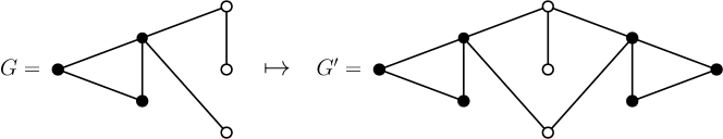
Figure 1. A graph $G$, and its doubled graph $G^{\prime}$, where the black and white dots denote interior and boundary vertices, respectively.

Definition 1.1.

Let $G^{\prime}=(V^{\prime},E^{\prime})$ be a doubled graph, and let $f:\mathring{V}\to U$ be an isomorphism as above, so that for all $w\in\partial V$ and $v\in\mathring{V},\ \{v,w\}\in E^{\prime}\iff\{f(v),w\}\in E^{\prime}.$ We say that a function $\varphi:V^{\prime}\rightarrow\mathbb{R}$ is even with respect to $\partial V$ if

$$\varphi(v)=\varphi(f(v))\text{ for }v\in\mathring{V},$$

and we say that $\varphi$ is odd with respect to $\partial V$ if

$$\varphi(v)=-\varphi(f(v))\text{ for }v\in\mathring{V},\quad\text{and}\quad\varphi(v)=0\text{ for }v\in\partial V.$$

Let $L^{\prime}:=D-A$ denote the graph Laplacian of $G^{\prime}$ where $D$ is the degree matrix of $G^{\prime}$, and $A$ is the adjacency matrix of $G^{\prime}$. The following proposition characterizes the eigenvectors of $L^{\prime}$ as either even or odd.

Proposition 1.1.

The graph Laplacian $L^{\prime}$ has $|V|$ eigenvectors that are even with respect to $\partial V$, and $|\mathring{V}|$ eigenvectors that are odd with respect to $\partial V$; this accounts for all eigenvectors of $L^{\prime}$.

1.2. Motivation

We are motivated by the observation that the restriction of the odd and even eigenvectors of $L^{\prime}$ to the graph $G$ seem like natural Dirichlet and Neumann Laplacian eigenvectors for the graph $G$, given the respective odd and even behavior of Dirichlet and Neumann Laplacian eigenfunctions on manifolds. In fact, the restriction of the odd eigenvectors of $L^{\prime}$ to the graph $G$ are eigenvectors of the Dirichlet graph Laplacian defined by Chung in [3], and inequalities involving the eigenvalues of this operator have been investigated [6]. However, an operator corresponding to the restriction of the even eigenvectors of $L^{\prime}$ to $G$ has not, to our knowledge been investigated. In [3], Chung defines the Neumann graph Laplacian by enforcing a condition that a discrete derivative vanishes on the boundary nodes of the graph, which results in different eigenvectors than those arising from the even eigenvectors of $L^{\prime}$. We note that a Cheeger inequality for Chung’s definition of the Neumann graph Laplacian has recently been established by Hua and Huang [8].

1.3. Odd and even eigenvectors

The proof of Proposition 1.1 gives some initial insight into the odd and even eigenvectors the graph Laplacian $L^{\prime}$ on the doubled graph $G^{\prime}$.

Proof of Proposition 1.1.

The proof of this proposition is immediate from the block structure of the graph Laplacian $L^{\prime}$. Indeed, let $L^{\prime}(U,W)$ denote the submatrix of $L^{\prime}$ whose rows and columns are indexed by $U\subseteq V$ and $W\subseteq V$, respectively. We can write

$$L^{\prime}=\left(\begin{array}[]{ccc}X&Y&0\\ Y^{\top}&Z&Y^{\top}\\ 0&Y&X\end{array}\right),$$

where $X$ is the submatrix $L^{\prime}(\mathring{V},\mathring{V})$, $Y$ is the submatrix $L^{\prime}(\mathring{V},\partial V)$, and $Z$ is the submatrix $L^{\prime}(\partial V,\partial V)$. With this notation, the eigenvectors of $L^{\prime}$ that are even with respect to $\partial V$ are solutions to the equation

$$\left(\begin{array}[]{ccc}X&Y&0\\ Y^{\top}&Z&Y^{\top}\\ 0&Y&X\end{array}\right)\left(\begin{array}[]{c}u\\ v\\ u\end{array}\right)=\mu\left(\begin{array}[]{c}u\\ v\\ u\end{array}\right).$$

That is to say, the vectors $u$ and $v$ satisfy $Xu+Yv=\mu u$ and $2Y^{\top}u+Zv=\mu v$. Put differently, when concatenated, $u$ and $v$ form an eigenvector of the matrix

(1) $$L_{R}:=\begin{pmatrix}X&Y\\ 2Y^{\top}&Z\end{pmatrix}.$$

Observe that $L_{R}$ is similar to a symmetric matrix

$$L_{R}=\begin{pmatrix}I&0\\ 0&\sqrt{2}I\end{pmatrix}\begin{pmatrix}X&\sqrt{2}Y\\ \sqrt{2}Y^{\top}&Z\end{pmatrix}\begin{pmatrix}I&0\\ 0&\sqrt{2}I\end{pmatrix}^{-1},$$

and thus by the Spectral Theorem, $L_{R}$ has $|V|$ real eigenvectors, which give rise to $|V|$ even eigenvectors of $L^{\prime}$. The eigenvectors of $L^{\prime}$ that are odd with respect to $\partial V$ are solutions to the equation

$$\left(\begin{array}[]{ccc}X&Y&0\\ Y^{\top}&Z&Y^{\top}\\ 0&Y&X\end{array}\right)\left(\begin{array}[]{c}u\\ 0\\ -u\end{array}\right)=\lambda\left(\begin{array}[]{c}u\\ 0\\ -u\end{array}\right).$$

Thus, each vector $u$ such that $Xu=\lambda u$ gives rise to an odd eigenvector of $L^{\prime}$. Let

$$L_{D}:=X.$$

Since $L_{D}$ is symmetric, it follows from the Spectral Theorem that it has $|\mathring{V}|$ real eigenvectors, and we conclude that $L^{\prime}$ has $|\mathring{V}|$ odd eigenvectors. ∎

1.4. Contribution

In this paper, we study the operator $L_{R}$ defined in (1) which we call the reflected Neumann graph Laplacian. This operator seems to be particularly natural on graphs approximating manifolds. For example, in Remark 1.1, we show that on the path graph, the eigenvectors of the Dirichlet graph Laplacian $L_{D}$ and reflected Neumann graph Laplacian $L_{R}$ are the familiar discrete sine and cosine functions. We remark that the definition of the reflected Neumann graph Laplacian $L_{R}$ has some similarities to the normalization used in the diffusion maps manifold learning method of Coifman and Lafon [7].

Our main result Theorem 1.1 shows that the first eigenvalue of the normalized reflected Neumann graph Laplacian $\mathcal{L}_{R}$ defined in (2) satisfies a Cheeger inequality. The graph cuts arising from $\mathcal{L}_{R}$ can differ significantly from graph cuts arising from the standard normalized graph Laplacian $\mathcal{L}$ defined in [3]. In Figure 3, we illustrate Theorem 1.1 with an example where the first eigenvector of the Neumann graph Laplacian $L_{R}$ suggests a drastically different cut than the first eigenvector of the standard graph Laplacian, and describe how the graph cut suggested by $L_{R}$ is consistent with the Cheeger inequality established in Theorem 1.1. It may be interesting to investigate the analog of other classical eigenvalue inequalities involving these definitions of $L_{D}$ and $L_{R}$ for graphs with boundary.

Remark 1.1.

The operators $L_{D}$ and $L_{R}$ are particularly natural on the path graph. Let $P_{n}=(V,E)$ denote the path graph on $n$ vertices, where $V=\{1,\ldots,n\}$ and $\{u,v\}\in E$ if and only if $|u-v|=1$. If $\partial V:=\{1,n\}$, then the doubled graph $P_{n}^{\prime}=C_{2n-2}$ is the cycle graph on $2n-2$ vertices, see Figure 2.

$\qquad\mapsto$

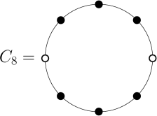
Figure 2. A path graph and its doubled graph.

Consider $L_{D}$ and $L_{R}$ of the path graph $P_{n}$. The Dirichlet eigenvectors $\varphi_{k}$ and eigenvalues $\lambda_{k}$, which satisfy $L_{D}\varphi_{k}=\lambda_{k}\varphi_{k}$ for $k=1,\ldots,n-2$, are of the form

$$\lambda_{k}:=2\left(1-\cos\left(\frac{\pi k}{n-1}\right)\right)\quad\text{and}\quad\varphi_{k}(j)=\sin\left(\frac{\pi jk}{n-1}\right),$$

for $j=1,\ldots,n-2$, while the Neumann eigenvectors, $\psi_{k}$ and $\mu_{k}$, which satisfy $L_{R}\psi_{k}=\mu_{k}\psi_{k}$ for $k=0,\ldots,n-1$, are of the form

$$\mu_{k}:=2\left(1-\cos\left(\frac{\pi k}{n-1}\right)\right)\quad\text{and}\quad\psi_{k}(j):=\cos\left(\frac{\pi jk}{n-1}\right)$$

for $j=0,\ldots,n-1$. Thus, the path graph doubling procedure defined in §1.1 gives the familiar sine and cosine functions, which are the Dirichlet and Neumann eigenfunctions of the Laplace operator of the unit interval.

1.5. Notation and definitions

Suppose that $G=(V,E)$ is a graph with vertices $V$ and edges $E$. Let $\partial V\subseteq V$ be a designated set of boundary vertices, and set $\mathring{V}=V\setminus\partial V$. We can write the adjacency matrix $A$ of the graph $G$ as the block matrix

$$A=\left(\begin{array}[]{cc}A_{11}&A_{12}\\ A_{12}^{\top}&A_{22}\end{array}\right),$$

where $A_{11}=A(\mathring{V},\mathring{V})$, $A_{12}=A(\mathring{V},\partial V)$, and $A_{22}=A(\partial V,\partial V)$. Motivated by Proposition 1.1 we define the reflected adjacency matrix $R$ by

$$R:=\left(\begin{array}[]{cc}A_{11}&A_{12}\\ 2A_{12}^{\top}&A_{22}\end{array}\right).$$

With this notation, the reflected Neumann Laplacian $L_{R}$ can be defined by

$$L_{R}=D-R,$$

where $D=\operatorname{diag}(R\vec{1})$, where $\vec{1}$ denotes a vector whose entries are all $1$, and whose dimensions are such that the matrix-vector multiplication is well defined. We define the normalized reflected Neumann graph Laplacian $\mathcal{L}_{R}$ by

(2) $$\mathcal{L}_{R}:=D^{-1/2}L_{R}D^{-1/2}.$$

1.6. Main result

In this section, we present our main result Theorem 1.1. While the matrix $\mathcal{L}_{R}$ is not in general symmetric, it is similar to a symmetric matrix; indeed, if

$$Q:=\left(\begin{array}[]{cc}I_{|\mathring{V}|}&0\\ 0&\frac{1}{2}I_{|\partial V|}\end{array}\right),$$

then $Q^{1/2}\mathcal{L}_{R}Q^{-1/2}$ is symmetric, positive-definite, and has the eigenvector $D^{1/2}Q^{1/2}\vec{1}$ of eigenvalue $0$. It follows that the first nontrivial eigenvalue $\lambda_{R}$ of $\mathcal{L}_{R}$ satisfies

$$\lambda_{R}:=\inf_{x^{\top}D^{1/2}Q^{1/2}\vec{1}=0}\frac{x^{\top}Q^{1/2}\mathcal{L}_{R}Q^{-1/2}x}{x^{\top}x}.$$

Let $E(U,W):=\left\{\{u,w\}\in E:u\in U,w\in W\right\}$, that is, $E(U,W)$ is the set of edges between $U$ and $W$. We define a measure $m(U,W)$ on this set of edges by

$$m(U,W)=|E(U,W)|-\frac{1}{2}|E(U\cap\partial V,W\cap\partial V)|,$$

and we define the volume $\operatorname{vol}(U)$ of $U\subseteq V$ by

$$\operatorname{vol}(U):=\sum_{u\in U}m(\{u\},V).$$

The following theorem is our main result.

Theorem 1.1.

Suppose that $G=(V,E)$ is a graph with a designated set of boundary vertices $\partial V\subseteq V$, and define the Cheeger constant $h_{R}$ by

(3) $$h_{R}:=\min_{S\subseteq V}\frac{m(S,V\setminus S)}{\min\{\operatorname{vol}(S),\operatorname{vol}(V\setminus S)\}}.$$

Then,

$$\sqrt{2\lambda_{R}}\geq h_{R}\geq\lambda_{R}/2,$$

where $\lambda_{R}$ is the first nontrivial eigenvalue of $\mathcal{L}_{R}$.

Recall that the standard Cheeger inequality is constructive in the sense that a cut that achieves the upper bound on the Cheeger constant can be determined from the eigenfunction corresponding to the first eigenvalue of the normalized graph Laplacian $\mathcal{L}$, see [1, 2]. Specifically, a partition that achieves the upper bound can be determined by dividing the vertices into two groups based on if the value of the first eigenvector is more or less than some threshold; for a detailed exposition see for example [3, 4]. Similarly, the result of Theorem 1.1 is constructive in the sense that a cut which achieves the upper bound on $h_{R}$ can be determined from the eigenvector $\psi_{R}$ of $\mathcal{L}_{R}$ that corresponds to $\lambda_{R}$. In the following remark, we present an example where the cut arising from $\psi_{R}$ differs significantly from the cut arising from the first eigenvector $\psi$ of the standard normalized graph Laplacian $\mathcal{L}$.

Remark 1.2.

Graph cuts arising from $\psi_{R}$ can differ significantly from graph cuts arising from $\psi$. Indeed, on the left of Figure 3 we illustrate a graph whose vertices are colored by greyscale values proportional to $\psi$. On the right of Figure 3 we illustrate the same graph except several vertices have been designated as boundary vertices (indicated by squares) and the color of the vertices is proportional to $\psi_{R}$. Observe that $\psi$ suggests cutting the graph by a vertical line into two equal parts, while $\psi_{R}$ suggests cutting the graph by a horizontal line into two equal parts.

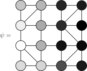
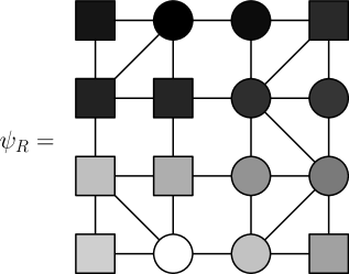
Figure 3. The same graph with vertices colored proportional to $\psi$ (left) and colored proportional to $\psi_{R}$ (right), where the squares in the right graph denote boundary vertices.

The fact that $\psi_{R}$ suggests a horizontal cut of the graph is illustrative of Theorem 1.1. Indeed, it is straightforward to check that the horizontal cut suggested by $\psi_{R}$ minimizes the cut measure $m(S,V\setminus S)/(\operatorname{vol}(S),\operatorname{vol}(V\setminus S)\})$ from (3). In contrast, the vertical cut suggested by $\psi$ minimizes the standard cut measure, which is equivalent to the measure $m(S,V\setminus S)/(\operatorname{vol}(S),\operatorname{vol}(V\setminus S)\})$ in the case that all vertices are interior vertices. Of course, Theorem 1.1 only guarantees that the measure of the cut arising from the eigenvector $\psi_{R}$ is an upper bound for $h_{R}$ with value at most $\sqrt{2\lambda_{R}}$; however, in this simple example the cut arising from $\psi_{R}$ actually obtains this minimum.

Remark 1.3.

Here we visualize the first eigenfunction $\psi_{R}$ of the reflected Neumann graph Laplacian $\mathcal{L}_{R}$ on a classic barbell shaped graph, see Figure 4.

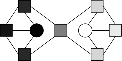
Figure 4. A barbell shaped graph whose vertices are colored proportional to $\psi_{R}$, where squares in the graph denote boundary vertices.

Observe that in Figure 4 the maximum and minimum value of the eigenvector occur at an interior vertex. This feature of the eigenvectors is interesting in the context of spectral clustering, where extreme values of the eigenvectors often correspond to the center of clusters.

1.7. Future Directions

One future direction for this work is the problem of selecting boundary vertices in a principled way. How the boundary is selected may depend on the application at hand. In a social network graph, boundary vertices could correspond to individuals with many connections outside the network. In the context of manifold learning, where the vertices of the graph are points in $\mathbb{R}^{n}$, boundary vertices could be selected based on the number of points within some $\varepsilon$-neighborhood of each vertex. On the other hand, when a graph is given by sampling from a pre-defined manifold with boundary, vertices selected from some collar neighborhood of the boundary could be designated as boundary vertices.

Another future direction arises from generalizing the setup under which our work was done. Our graph doubling procedure inputs a graph with boundary and outputs a larger graph, containing the original graph as an induced subgraph, which has a special $Z_{2}$ symmetry. Could similar Cheeger results be proven for other reflection procedures? For example, what if $n-1$ copies of the interior vertices were attached, instead of only 1?

Finally, we note a connection between the doubled graph (defined in §1.1) and numerical analysis, that may motivate a direction for future study. Recall that for a path graph $P_{n}$ the eigenfunctions of the reflected Neumann Laplacian $L_{R}$ are of the form $\psi_{k}(j)=\cos(\pi jk/(n-1))$, see Remark 1.1. These Neumann eigenvectors are precisely the basis vectors for the Discrete Cosine Transform (DCT) Type I, as classified in [9]. The DCT Type II, which has basis vectors $\psi_{k}(j)=\cos(\pi(j+1/2)k/n)$ is also important in numerical analysis; it could be interesting to develop a graph doubling procedure whose Neumann eigenvectors on the path graph are these vectors.

2. Proof of Main Result

2.1. Summary

The proof of Theorem 1.1 is divided into two lemmas: first, in Lemma 2.1 we show that $\lambda_{R}\leq 2h_{R}$, and second, in Lemma 2.2 we show that $h_{R}^{2}/2\leq\lambda_{R}$. The structure of our argument is similar to classical Cheeger inequality proofs, see [3, 5].

2.2. Proof of Theorem 1.1

Lemma 2.1 (Trivial direction).

We have

$$\lambda_{R}\leq 2h_{R}.$$

Proof of Lemma 2.1.

Recall that

$$\mathcal{L}_{R}:=D^{-1/2}Q^{1/2}L_{R}Q^{-1/2}D^{-1/2}.$$

First, we observe that $QL_{R}$ can be written as

$$QL_{R}=L-\frac{1}{2}L_{\partial},$$

where

$$L=\left(\begin{array}[]{cc}\operatorname{diag}(A_{11}\vec{1}+A_{12}\vec{1})-A_{11}&-A_{12}\\ -A_{12}^{\top}&\operatorname{diag}(A_{12}^{\top}\vec{1}+A_{22}\vec{1})-A_{22}\end{array}\right),$$

and

$$L_{\partial}:=\left(\begin{array}[]{cc}0&0\\ 0&\operatorname{diag}(A_{22}\vec{1})-A_{22}\end{array}\right).$$

Observe that $L$ is the standard graph Laplacian of $G$, while $L_{\partial}$ is the graph Laplacian of the vertex induced subgraph $G[\partial V]$. Fix a subset $S\subseteq V$, and let $\chi_{S}$ be the indicator function for $S$. Define

$$x:=Q^{1/2}D^{1/2}\chi_{S}-\frac{\chi_{S}^{\top}DQ\vec{1}}{\vec{1}^{\top}DQ\vec{1}}D^{1/2}Q^{1/2}\vec{1}.$$

By construction, we have $x^{\top}D^{1/2}Q^{1/2}\vec{1}=0$, and it follows that

$$\lambda_{N} \leq \frac{x^{\top}D^{-1/2}Q^{1/2}L_{R}Q^{-1/2}D^{-1/2}x}{x^{\top}x}$$

$$= \frac{\chi_{S}^{\top}QL_{R}\chi_{S}}{\chi_{S}^{\top}DQ\chi_{S}\left(\vec{1}-\frac{\chi_{S}^{\top}DQ\chi_{S}}{\vec{1}^{\top}DQ1}\right)}$$

$$= \frac{\chi_{S}^{\top}(L-\frac{1}{2}L_{\partial})\chi_{S}\left(\vec{1}^{\top}DQ\vec{1}\right)}{\left(\chi_{S}^{\top}DQ\chi_{S}^{\top}\right)\left(\chi_{V\setminus S}^{\top}DQ\chi_{V\setminus S}\right)}$$

$$\leq \frac{2\cdot\chi_{S}^{\top}(L-\frac{1}{2}L_{\partial})\chi_{S}}{\min\left\{\left(\chi_{S}^{\top}DQ\chi_{S}^{\top}\right),\left(\chi_{V\setminus S}^{\top}DQ\chi_{V\setminus S}\right)\right\}}$$

$$= \frac{2\cdot m(S,V\setminus S)}{\min\{\operatorname{vol}(S),\operatorname{vol}(V\setminus S)\}}.$$

Since this inequality holds for all subsets $S\subseteq V$, we conclude that $\lambda_{R}\leq 2h_{R}$, as was to be shown. ∎

Lemma 2.2 (Nontrivial direction).

We have

$$\lambda_{R}\geq\frac{h_{R}^{2}}{2}.$$

Proof of Lemma 2.2.

Recall that

$$\lambda_{R}=\inf_{x^{\top}D^{1/2}Q^{1/2}\vec{1}=0}\frac{x^{\top}\mathcal{L}_{R}x}{x^{\top}x}=\inf_{y^{\top}DQ\vec{1}=0}\frac{y^{\top}QL_{R}y}{y^{\top}QDy}.$$

Let $g$ be a vector satisfying

$$\lambda_{R}=\frac{g^{\top}QL_{R}g}{g^{\top}DQg},\quad\text{and}\quad g^{\top}QD\vec{1}=0.$$

Let $\{v_{1},\ldots,v_{n}\}$ be an enumeration of the vertices $V$ so that $g_{v_{1}}\leq...\leq g_{v_{n}}$, and set $S_{j}:=\{v_{1},...,v_{j}\}$, for $j=1,\ldots,n.$ Let $p$ be the largest integer such that $\operatorname{vol}(S_{p})\leq\operatorname{vol}(V)/2$, that is,

$$p:=\max\left\{j\in\{1,\ldots,n\}:\text{vol}(S_{j})\leq\text{vol}(V)/2\right\}.$$

Let $g^{+}$ and $g^{-}$ denote the positive and negative parts of $g-g_{v_{p}}$, respectively. That is, $g^{+}_{v}:=\max\{g_{v}-g_{v_{p}},0\}$ and $g^{-}_{v}:=\max\{g_{v_{p}}-g_{v},0\}.$ Let $u\sim v$ denote $\{u,v\}\in E$ and $q=\operatorname{diag}(Q).$ Then

$$\lambda_{R} = \frac{g^{\top}(L-\frac{1}{2}L_{\partial})g}{g^{\top}DQg}$$

$$= \frac{\sum_{u\sim v}(g_{u}-g_{v})^{2}-\frac{1}{2}\sum_{\begin{subarray}{c}u\sim v\\ u,v\in\partial V\end{subarray}}(g_{u}-g_{v})^{2}}{\sum_{v}g_{v}^{2}d_{v}q_{v}}$$

$$\geq \frac{\sum_{u\sim v}(g_{u}-g_{v})^{2}-\frac{1}{2}\sum_{\begin{subarray}{c}u\sim v\\ u,v\in\partial V\end{subarray}}(g_{u}-g_{v})^{2}}{\sum_{v}(g(v)-g(v_{p}))^{2}d_{v}q_{v}},$$

where the last inequality holds because we have increased the denominator. From here,

(4) $$\lambda_{R}\geq\frac{\sum_{u\sim v}((g^{+}_{u}-g^{+}_{v})^{2}+(g^{-}_{u}-g^{-}_{v})^{2})-\frac{1}{2}\sum_{\begin{subarray}{c}u\sim v\\ u,v\in\partial V\end{subarray}}((g^{+}_{u}-g^{+}_{v})^{2}+(g^{-}_{u}-g^{-}_{v})^{2})}{\sum_{v}((g^{+}_{v})^{2}+(g^{-}_{v})^{2})d_{v}q_{v}},$$

Recall that

(5) $$\frac{a+b}{c+d}\geq\text{min}\left\{\frac{a}{c},\frac{b}{d}\right\},$$

for any $a,b\geq 0$ and $c,d>0$. From (4), we can set $a=\sum_{u\sim v}(g^{+}_{u}-g^{+}_{v})^{2}-\sum_{\begin{subarray}{c}u\sim v\\ u,v\in\partial V\end{subarray}}(g^{+}_{u}-g^{+}_{v})^{2},$ $b=\sum_{u\sim v}(g^{-}_{u}-g^{-}_{v})^{2}-\sum_{\begin{subarray}{c}u\sim v\\ u,v\in\partial V\end{subarray}}(g^{-}_{u}-g^{-}_{v})^{2},$ $c=\sum_{v}(g^{+}_{v})^{2}d_{v}q_{v},$ and $d=\sum_{v}(g^{-}_{v})^{2}d_{v}q_{v}.$ Observe that $a$ and $b$ are nonnegative. Indeed,

$$a=\sum_{\begin{subarray}{c}u\sim v\\ u\notin\partial V\ \text{or}\ v\notin\partial V\end{subarray}}(g^{+}_{u}-g^{+}_{v})^{2},$$

which has nonnegative summands, and a similar statement holds for $b.$

Without loss of generality, (5) implies that

$$\lambda_{R}\geq\frac{\sum_{u\sim v}(g^{+}_{u}-g^{+}_{v})^{2}-\frac{1}{2}\sum_{\begin{subarray}{c}u\sim v\\ u,v\in\partial V\end{subarray}}(g^{+}_{u}-g^{+}_{v})^{2}}{\sum_{v}(g^{+}_{v})^{2}d_{v}q_{v}}.$$

To simplify notation in the following, let $f=g^{+}$. We begin by setting

$$\lambda:=\frac{\sum_{u\sim v}(f_{u}-f_{v})^{2}-\frac{1}{2}\sum_{\begin{subarray}{c}u\sim v\\ u,v\in\partial V\end{subarray}}(f_{u}-f_{v})^{2}}{\sum_{v}f_{v}^{2}d_{v}q_{v}}.$$

Multiplying the numerator and denominator by the same term gives

$$\lambda=\frac{\left(\sum_{u\sim v}(f_{u}-f_{v})^{2}-\frac{1}{2}\sum_{\begin{subarray}{c}u\sim v\\ u,v\in\partial V\end{subarray}}(f_{u}-f_{v})^{2}\right)\left(\sum_{u\sim v}(f_{u}+f_{v})^{2}-\frac{1}{2}\sum_{\begin{subarray}{c}u\sim v\\ u,v\in\partial V\end{subarray}}(f_{u}+f_{v})^{2}\right)}{\left(\sum_{v}f_{v}^{2}d_{v}q_{v}\right)\left(\sum_{u\sim v}(f_{u}+f_{v})^{2}-\frac{1}{2}\sum_{\begin{subarray}{c}u\sim v\\ u,v\in\partial V\end{subarray}}(f_{u}+f_{v})^{2}\right)}.$$

Applying the Cauchy-Schwarz inequality in the numerator gives

$$\lambda\geq\frac{\left(\sum_{u\sim v}|f_{u}^{2}-f_{v}^{2}|-\frac{1}{2}\sum_{\begin{subarray}{c}u\sim v\\ u,v\in\partial V\end{subarray}}|f_{u}^{2}-f_{v}^{2}|\right)^{2}}{\left(\sum_{v}f_{v}^{2}d_{v}q_{v}\right)\left(\sum_{u\sim v}(f_{u}+f_{v})^{2}-\frac{1}{2}\sum_{\begin{subarray}{c}u\sim v\\ u,v\in\partial V\end{subarray}}(f_{u}+f_{v})^{2}\right)}.$$

Next, we observe that

$$\sum_{u\sim v}(f_{u}+f_{v})^{2}-\frac{1}{2}\sum_{\begin{subarray}{c}u\sim v\\ u,v\in\partial V\end{subarray}}(f_{u}+f_{v})^{2}=\sum_{v}f_{v}^{2}d_{v}q_{v}-\left(\sum_{u\sim v}(f_{u}-f_{v})^{2}-\frac{1}{2}\sum_{\begin{subarray}{c}u\sim v\\ u,v\in\partial V\end{subarray}}(f_{u}-f_{v})^{2}\right),$$

and thus it follows that

$$\lambda\geq\frac{\left(\sum_{u\sim v}|f_{u}^{2}-f_{v}^{2}|-\frac{1}{2}\sum_{\begin{subarray}{c}u\sim v\\ u,v\in\partial V\end{subarray}}|f_{u}^{2}-f_{v}^{2}|\right)^{2}}{\left(\sum_{v}f_{v}^{2}d_{v}q_{v}\right)^{2}\left(2-\lambda\right)}.$$

We want to show that

$$\sum_{u\sim v}|f_{u}^{2}-f_{v}^{2}|-\frac{1}{2}\sum_{\begin{subarray}{c}u\sim v\\ u,v\in\partial V\end{subarray}}|f_{u}^{2}-f_{v}^{2}|\geq\sum_{i=1}^{n}|f_{v_{i}}^{2}-f_{v_{i+1}}^{2}|m(S_{i},V\setminus S_{i}).$$

We can write

$$\sum_{u\sim v}|f_{u}^{2}-f_{v}^{2}|-\frac{1}{2}\sum_{\begin{subarray}{c}u\sim v\\ u,v\in\partial V\end{subarray}}|f_{u}^{2}-f_{v}^{2}|=\sum_{i=2}^{n}\sum_{j=1}^{i-1}\left(\chi_{E_{i,j}}-\frac{1}{2}\chi_{\partial_{i}}\chi_{\partial_{j}}\right)(f_{v_{i}}^{2}-f_{v_{j}}^{2}),$$

where

$$\chi_{E_{i,j}}=\begin{cases}1\ \text{if}\ \{v_{i},v_{j}\}\in E\\ 0\ \text{otherwise}\end{cases}$$

is the indicator function for $\{v_{i},v_{j}\}\in E$, and

$$\chi_{\partial_{i}}=\begin{cases}1\ \text{if}\ i\in\partial V\\ 0\ \text{otherwise}\end{cases}$$

is the indicator function for $v_{i}\in\partial V$. Note that we are justified in dropping the absolute value signs because $f_{v_{i}}^{2}$ is an increasing function of $i.$ Next we write $f_{v_{i}}^{2}-f_{v_{j}}^{2}$ as a telescoping series

$$f_{v_{i}}^{2}-f_{v_{j}}^{2}=(f_{v_{i}}^{2}-f_{v_{i-1}}^{2})+(f_{v_{i-1}}^{2}-f_{v_{i-2}}^{2})+...+(f_{v_{j+1}}^{2}-f_{v_{j}}^{2}),$$

and rearrange terms in the summation to conclude that

$$\sum_{i=2}^{n}\sum_{j=1}^{i-1}\left(\chi_{E_{i,j}}-\frac{1}{2}\chi_{\partial_{i}}\chi_{\partial_{j}}\right)(f_{v_{i}}^{2}-f_{v_{j}}^{2})=\\ \sum_{l=1}^{n}\sum_{k=1}^{n}\sum_{j=1}^{n}\left(\left(\chi_{E_{j,k+l}}-\frac{1}{2}\chi_{\partial_{j}}\chi_{\partial_{k+l}}\right)\chi_{j\leq l}\right)(f_{v_{l+1}}^{2}-f_{v_{l}}^{2}),$$

where

$$\chi_{j\leq l}=\begin{cases}1\ \text{if}\ j\leq l\\ 0\ \text{otherwise}.\end{cases}$$

Then, to complete this step, we note that

$$\sum_{k=1}^{n}\sum_{j=1}^{n}\left(\left(\chi_{E_{j,k+l}}-\frac{1}{2}\chi_{\partial_{j}}\chi_{\partial_{k+l}}\right)\chi_{j\leq l}\right)=m(S_{l},V\setminus S_{l}).$$

Returning to our main sequence of inequalities for $\lambda$, we have

$$\lambda \geq \frac{(\sum_{i}|f_{v_{i}}^{2}-f_{v_{i+1}}^{2}|m(S_{i},V\setminus S_{i}))^{2}}{2(\sum_{v}f_{v}^{2}d_{v}q_{v})^{2}}$$

$$\geq \frac{(\alpha\sum_{i=1}^{n}|f_{v_{i}}^{2}-f_{v_{i+1}}^{2}|\min\{\text{vol}(S_{i}),\text{vol}(V\setminus S_{i})\})^{2}}{2(\sum_{u}f(u)^{2}d_{u}q_{v})^{2}},$$

where

$$\alpha:=\min_{1\leq i\leq n}\frac{m(S_{i},V\setminus S_{i})}{\min\{\operatorname{vol}(S_{i}),\operatorname{vol}(V\setminus S_{i})\}}.$$

Since $f_{v_{i}}^{2}$ is nondecreasing, a rearrangement of the numerator of the previous expression gives

$$\lambda\geq\frac{\alpha^{2}}{2}\frac{(\sum_{i}(f_{v_{i}}^{2}|\min\{\operatorname{vol}(S_{i}),\text{vol}(V\setminus S_{i})\}-\min\{\operatorname{vol}(S_{i+1}),\text{vol}(V\setminus S_{i+1})\}|))^{2}}{(\sum_{u}f(u)^{2}d_{u}q_{u})^{2}}.$$

It follows that

$$\lambda_{R}\geq\lambda\geq\frac{\alpha^{2}}{2}\frac{(\sum_{i}f_{v_{i}}^{2}d_{v_{i}}q_{v_{i}})^{2}}{(\sum_{u}f_{u}^{2}d_{u}q_{u})^{2}}=\frac{\alpha^{2}}{2}\geq\frac{h_{R}^{2}}{2},$$

which completes the proof. ∎

Acknowledgements

We thank the referees for their helpful comments. This research was supported by Summer Undergraduate Math Research at Yale (SUMRY) 2018. NFM was supported in part by NSF DMS-1903015.

References

- [1] N. Alon. Eigenvalues and expanders. Combinatorica, 6 (1986): 86–96.
- [2] J. Cheeger. A lower bound for the smallest eigenvalue of the Laplacian. Problems in Analysis, R. C. Gunning, editor, Princeton Univ. Press, (1970): 195-199.
- [3] F. Chung. Spectral Graph Theory. CBMS Regional Conference Series in Mathematics, No. 92, American Mathematical Society, 1997.
- [4] F. Chung. Four Cheeger-type inequalities for graph partitioning algorithms. Proc. ICCM, 2 (2007): 751–772.
- [5] F. Chung. Laplacians of graphs and Cheeger’s inequalities. Combinatorics, Paul Erdos is eighty, 2 (1996): 157–172.
- [6] F. Chung and K. Oden. Weighted Graph Laplacians and Isoperimetric Inequalities. Pac. J. Appl. Math. 192, no. 2 (2000): 257–273.
- [7] R. R. Coifman and S. S. Lafon. Diffusion maps. Appl. Comput. Harmon. Anal., 21, no. 1 (2006): 5–30.
- [8] B. Hua and Y. Huang. Neumann Cheeger Constants on Graphs. J. Geom. Anal., 28 (2018): 2166–2184.
- [9] G. Strang. The Discrete Cosine Transform. SIAM Rev., 41 (1999): 135–147.