Deep Mixtures of Unigrams for uncovering Topics in Textual Data

Abstract

Mixtures of Unigrams are one of the simplest and most efficient tools for clustering textual data, as they assume that documents related to the same topic have similar distributions of terms, naturally described by Multinomials. When the classification task is particularly challenging, such as when the document-term matrix is high-dimensional and extremely sparse, a more composite representation can provide better insight on the grouping structure. In this work, we developed a deep version of mixtures of Unigrams for the unsupervised classification of very short documents with a large number of terms, by allowing for models with further deeper latent layers; the proposal is derived in a Bayesian framework. The behaviour of the Deep Mixtures of Unigrams is empirically compared with that of other traditional and state-of-the-art methods, namely $k$-means with cosine distance, $k$-means with Euclidean distance on data transformed according to Semantic Analysis, Partition Around Medoids, Mixture of Gaussians on semantic-based transformed data, hierarchical clustering according to Ward’s method with cosine dissimilarity, Latent Dirichlet Allocation, Mixtures of Unigrams estimated via the EM algorithm, Spectral Clustering and Affinity Propagation clustering. The performance is evaluated in terms of both correct classification rate and Adjusted Rand Index. Simulation studies and real data analysis prove that going deep in clustering such data highly improves the classification accuracy.

Keywords: Deep learning Mixture models Clustering Text Data Analysis

1 Introduction

Deep learning methods are receiving an exponentially increasing interest in the last years as powerful tools to learn complex representations of data. They can be basically defined as a multi-layer stack of algorithms or modules able to gradually learn a huge number of parameters in an architecture composed by multiple nonlinear transformations (LeCun et al., 2015). Typically, and for historical reasons, a structure for deep learning is identified with advanced neural networks: deep Feed Forward, Recurrent, Auto-encoder, Convolution neural networks are very effective and used algorithms of deep learning (Schmidhuber, 2015). They demonstrated to be particularly successful in supervised classification problems arising in several fields such as image and speech recognition, gene expression data, topic classification. Under the framework of graph-based learning, Peng et al. (2016) proposed an efficient method to produce robust subspace clustering and subspace learning; deep model-Structured AutoEncoder for subspace clustering were introduced by Peng et al. (2018) to map input data points into nonlinear latent spaces while preserving the local and global subspace structure. Zhou et al. (2018) addressed the data sparsity issue in hashing.

When the aim is uncovering unknown classes in an unsupervised classification perspective, important methods of deep learning have been developed along the lines of mixture modeling, because of their ability to decompose a heterogeneous collection of units into a finite number of sub-groups with homogeneous structures (Fraley and Raftery, 2002; McLachlan and Peel, 2000). In this direction, van den Oord and Schrauwen (2014) proposed Multilayer Gaussian Mixture Models for modeling natural images; Tang et al. (2012) defined deep mixture of factor analyzers with a greedy layer-wise learning algorithm able to learn each layer at a time. Viroli and McLachlan (2019) developed a general framework for Deep Gaussian mixture models that generalizes and encompasses the previous strategies and several flexible model-based clustering methods such as mixtures of mixture models (Li, 2005), mixtures of Factor Analyzers (McLachlan et al., 2003), mixtures of factor analyzers with common factor loadings (Baek et al., 2010), heteroscedastic factor mixture analysis (Montanari and Viroli, 2010) and mixtures of factor mixture analyzers introduced by Viroli (2010). A general ‘take-home-message’ coming from the existing deep clustering strategies is that deep methods vs shallow ones appear to be very efficient and powerful tools especially for complex high-dimensional data; on the contrary, for simple and small data structures, a deep learning strategy cannot improve performance of simpler and conventional methods or, to better say, it is like to use a ‘sledgehammer to crack a nut’ (Viroli and McLachlan, 2019).

The motivating problem behind this work derives from ticket data (i.e. content of calls made to the customer service) of an important mobile phone company, collected in Italian language. When a customer calls the assistance service, a ticket is created: the agent classifies it as e.g. a claim, a request of information for specific services, deals or promotions. Our dataset consists of tickets related to five classes of services, previously classified from independent operators. The aim is to define an efficient clustering strategy to automatically assign the tickets into the same classes without the human judgment of an operator. The data are textual and information are collected in a document-term matrix with raw frequencies at each cell. They have a very complex and a high-dimensional structure, caused by the huge number of tickets and terms used by people that call the company for a specific request and by a relevant degree of sparsity (after a pre-processing step, the tickets have indeed an average length of only 5 words and, thus, the document-term matrix contains zero almost everywhere).

The simplest topic model for clustering document-term data is represented by Mixture of Unigrams (MoU, Nigam et al., 2000), based on the idea of modeling the word frequencies as multinomial distributions, under the assumption that a document refers to a single topic. Table 7 shows that on the ticket dataset this method appears to be the most efficient tool for classifying the complex ticket data, compared to other conventional clustering strategies such as $k$-means, Partition Around Medoids and hierarchical clustering. The reason is probably related to the fact that, by using proportions, MoU is not affected by the large amount of zeros, differently from the other competitors. We also compared MoU with the Latent Dirichlet Allocation model (LDA, Blei et al., 2003), which represents an important and very popular model in textual data analysis, allowing documents to exhibit multiple topics with a different degree of importance. The Latent Dirichlet Allocation model has demonstrated great success on long texts (Griffiths and Steyvers, 2004), and it could be thought of as a generalization of the MoU, because it adds a hierarchical level to it and, hence, much more flexibility. However, when dealing with very short documents like the ticket dataset, it is very rare that a single unit could refer to more than one topic; in such cases, the LDA model may not improve the clustering performance of MoU.

The aim of this paper is to derive a deep generalization of Mixtures of Unigrams, in order to better uncover topics or groups in case of complex and high-dimensional data. The proposal will be derived in a Bayesian framework and we will show that it will be particularly efficient for classifying the ticket data with respect to the ‘shallow’ MoU model. We will also show the good performance of the proposed method in a simulation study.

The paper is organized as follows. In the next section the mixture of unigrams model is described. In Section 3 the deep formulation of the model is developed. Section 4 is devoted to the estimation algorithm for fitting the model. Experimental results on simulated and real data are presented in Sections 5 and 6, respectively. We conclude the paper with some final remarks (Section 7).

2 Mixtures of Unigrams

Let ${\bf X}$ be a document-term matrix of dimension $n\times T$ containing the word frequencies of each document in row and let $k$ be the number of homogeneous groups in which documents could be allocated. Let ${\bf x}_{d}$ be the single document of length $T$, with $d=1,\ldots,n$.

In MoU the distribution of each document has a specific distribution function conditional on the values of a discrete latent allocation variable $z_{d}$ describing the probability of each topic. More precisely,

$$p({\bf x}_{d})=\sum_{i=1}^{k}\pi_{i}p({\bf x}_{d}|z_{d}=i),$$ (1)

with $p(z_{d}=i)=\pi_{i}$, under the restrictions (i) $\pi_{i}>0$ for $i=1,\ldots,k$ and (ii) $\sum_{i=1}^{k}\pi_{i}=1$.

The natural distribution for $p({\bf x}_{d}|z_{d}=i)$ is represented by the multinomial distribution with a parameter vector, say $\bm{\omega}_{i}$, that is cluster-specific:

$$p({\bf x}_{d}|z_{d}=i)=\frac{N_{d}!}{\prod_{t=1}^{T}x_{dt}!}\prod_{t=1}^{T}\omega_{ti}^{x_{dt}},$$

with $N_{d}=\sum_{t=1}^{T}x_{dt}$ denoting the word-length of the document $d$. The multinomial distribution assumes that, conditionally to the cluster membership, all the terms can be regarded as independently distributed.

The model is indeed a simple mixture of multinomial distributions that can be easily estimated by the EM algorithm (see Nigam et al., 2000, for further details) under the assumption that a document belongs to a single topic and the number of groups coincides with the number of topics. The approach has been successfully applied not only to textual data, where it originated from, but to genomic data analysis. In this latter field a particular improvement of the method consists in relaxing the conditional independence assumption of the variables/terms, by using $m$-order Markov properties, thus leading to the so-called m-gram models (Tomović et al., 2006). Due to the limited average length of documents in ticket data, co-occurrence information is very rare and this extension would be not effective on these data.

3 Going deep into mixtures of unigrams: a novel approach

We aim at extending MoU by allowing a further layer in the probabilistic generative model, so as to get a nested architecture of nonlinear transformations able to describe the data structure in a very flexible way. At the deepest latent layer, the documents can come from $k_{2}$ groups with different probabilities, say $\pi_{j}^{(2)}\ \ j=1,\ldots,k_{2}$. Conditionally to what happened at this level, at the top observable layer the documents can belong to $k_{1}$ groups with conditional probabilities $\pi_{i|j}^{(1)}\ \ i=1,\ldots,k_{1}$. For the sake of a simple notation, we refer in the following to a generic document denoted by ${\bf x}$. The distribution of ${\bf x}$ conditionally to the two layers is a multinomial distribution with cluster-specific proportions $\bm{\omega}$:

$$p({\bf x}|z^{(1)}=i,z^{(2)}=j,\bm{\omega})=\frac{\left(\sum_{t=1}^{T}x_{t}\right)!}{\prod_{t=1}^{T}x_{t}!}\prod_{t=1}^{T}\omega_{tij}^{x_{t}},$$ (2)

where $z^{(1)}$ and $z^{(2)}$ are the allocation variables at the top and at the bottom layers, respectively. They are discrete latent variables that follow the distributions:

$$p(z^{(2)}=j)=\pi_{j}^{(2)},$$ (3)

and

$$p(z^{(1)}=i|z^{(2)}=j)=\pi_{i|j}^{(1)}.$$ (4)

In mixture of unigrams the proportions $\bm{\omega}$ were fixed parameters. Here we assume they are realizations of random variables with a Dirichlet distribution. In order to have a flexible and deep model we assume that the parameters of the Dirichlet distribution are a linear function of two sets of parameters that originate in the two subsequent layers. The Dirichlet parameters are $\bm{\beta}_{i}+\bm{\alpha}_{j}\bm{\beta}_{i}=\bm{\beta}_{i}(1+\bm{\alpha}_{j})$, where $\bm{\beta}_{i}$ and $\bm{\alpha}_{j}$ are vectors of length $T$. Since they must be positive and the overall model must be identifiable, we further assume that $\beta_{it}>0$ and $-1<\alpha_{jt}<1$. These choices lead to a nice interpretative perspective: at the bottom layer $\bm{\alpha}_{j}$ acts as a perturbation on the cluster-specific $\bm{\beta}_{i}$ parameters of the top layer. Therefore the distribution is:

$$p(\bm{\omega}|z^{(1)}=i,z^{(2)}=j)=\frac{\Gamma\left(\sum_{t=1}^{T}\beta_{it}(1+\alpha_{jt})\right)}{\prod_{t=1}^{T}\Gamma(\beta_{it}(1+\alpha_{jt}))}\prod_{t=1}^{T}\omega_{tij}^{\beta_{it}(1+\alpha_{jt})-1},$$ (5)

where $\Gamma$ denotes the Gamma function.

An example of Deep MoU structure is depicted in Figure 1 for the case $k_{1}=3$ and $k_{2}=2$. Notice that in a model with $k_{1}=3$ and $k_{2}=2$ components we have an overall number $M$ of sub-components equal to 5, but $6>M$ possible paths for each document. The paths share and combine the parameters of the two levels, thus achieving great flexibility with less parameters to be estimated.

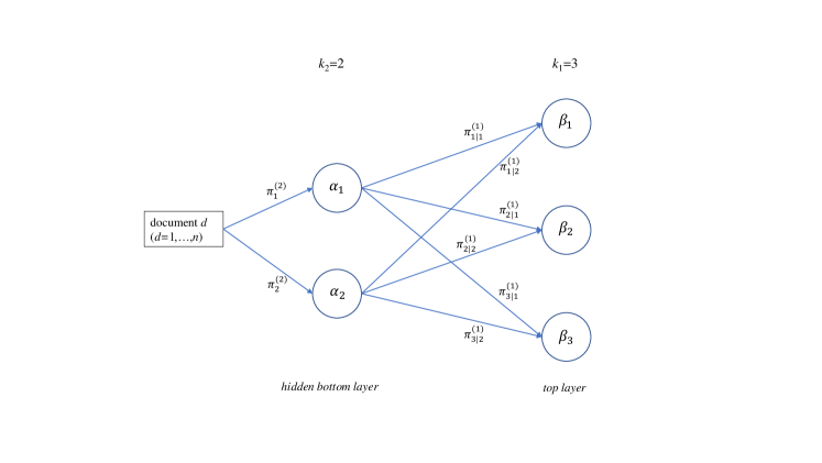
Figure 1: Structure of a Deep MoU with components $k_{1}=3$ and $k_{2}=2$.

By combining equations (2) and (5), the latent variable $\bm{\omega}$ can be integrated out from the model estimation, thus gaining efficiency without losing flexibility and interpretability. More precisely:

$$\begin{aligned} p&({\bf x}|z^{(1)}=i,z^{(2)}=j)\\ &=\int p({\bf x}|z^{(1)}=i,z^{(2)}=j,\bm{\omega})p(\bm{\omega}|z^{(1)}=i,z^{(2)}=j)d\bm{\omega}\\ &=\frac{\left(\sum_{t=1}^{T}x_{t}\right)!}{\prod_{t=1}^{T}x_{t}!}\frac{\Gamma\left(\sum_{t=1}^{T}\beta_{it}(1+\alpha_{jt})\right)}{\prod_{t=1}^{T}\Gamma(\beta_{it}(1+\alpha_{jt}))}\int\prod_{t=1}^{T}\omega_{tij}^{x_{t}+\beta_{it}(1+\alpha_{jt})-1}d\bm{\omega}_{ij}\\ &=\frac{\left(\sum_{t=1}^{T}x_{t}\right)!}{\prod_{t=1}^{T}x_{t}!}\frac{\Gamma\left(\sum_{t=1}^{T}\beta_{it}(1+\alpha_{jt})\right)}{\prod_{t=1}^{T}\Gamma(\beta_{it}(1+\alpha_{jt}))}\frac{\prod_{t=1}^{T}x_{t}+\Gamma(\beta_{it}(1+\alpha_{jt}))}{\Gamma\left(\sum_{t=1}^{T}x_{t}+\beta_{it}(1+\alpha_{jt})\right)}\\ &=\frac{\sum_{t=1}^{T}x_{t}}{\prod_{t=1}^{T}x_{t}}\frac{B\left(\sum_{t=1}^{T}x_{t},\sum_{t=1}^{T}\beta_{it}(1+\alpha_{jt})\right)}{\prod_{t=1}^{T}B\left(x_{t},\beta_{it}(1+\alpha_{jt})\right)},\end{aligned}$$ (6)

where $B$ denotes the Beta function.

Figure 2 shows the Directed Acyclic Graph (DAG) summarizing the dependence structure of the model.

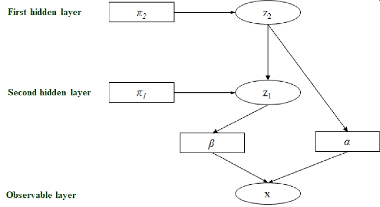
Figure 2: DAG specifying the Deep MoU model.

Finally by combining formulas (6) with (3) and (4), the density of the data is a mixture of mixtures of Multinomial-Dirichlet distributions:

$$p({\bf x})=\sum_{i=1}^{k_{1}}\sum_{j=1}^{k_{2}}\pi_{i|j}^{(1)}\pi_{j}^{(2)}\frac{\sum_{t=1}^{T}x_{t}}{\prod_{t=1}^{T}x_{t}}\frac{B\left(\sum_{t=1}^{T}x_{t},\sum_{t=1}^{T}\beta_{it}(1+\alpha_{jt})\right)}{\prod_{t=1}^{T}B\left(x_{t},\beta_{it}(1+\alpha_{jt})\right)}.$$ (7)

In other terms, adding a level to the hierarchy resulted in adding a mixing step. A double mixture is deeper, more flexible and it can capture more heterogeneity of the data, than a simple mixture of Multinomial-Dirichlet distributions. Having two layers and two number of groups for each, that are $k_{1}$ and $k_{2}$, it is important to define the procedure by which the units are clustered.

3.1 Cluster assignment

Theoretically, under this double mixtures, we could group units into $k_{1}$ groups, $k_{2}$ groups or $k_{1}\times k_{2}$ groups. However, note that, under the constraint $-1<\alpha_{jt}<1$, the role of $k_{2}$ components at the deepest layer is confined to add flexibility to the model, while the real cluster-distribution is specified by the $\bm{\beta}$ parameters. For this reason, the number of ‘real’ clusters is given by $k_{1}$. Their internal heterogeneity is captured by the $k_{2}$ sub-groups that help in adding more flexibility to the model. Therefore, the final allocation of the documents to the clusters is thus given by the posterior probability $p(z^{(1)}|{\bf x})$ that can be obtained as follows:

$$p(z^{(1)}=i|{\bf x})=\frac{\sum_{j=1}^{k_{2}}\pi_{i|j}^{(1)}\pi_{j}^{(2)}p({\bf x}|z^{(1)}=i,z^{(2)}=j)}{\sum_{i=1}^{k_{1}}\sum_{j=1}^{k_{2}}\pi_{i|j}^{(1)}\pi_{j}^{(2)}p({\bf x}|z^{(1)}=i,z^{(2)}=j)}.$$ (8)

The model encompasses the simple MoU, that can be obtained as special case when $k_{2}=1$ and without any prior on $\bm{\omega}$. When $k_{2}=1$ and a Dirichlet prior is put on $\bm{\omega}$ a mixture of Dirichlet-Multinomial is defined. In this case, in order to assure identifiability, we assume $\bm{\alpha}=0$.

The approach can be generalized to multilayer of latent variables, where at each layer perturbation parameters to the final $\bm{\beta}$ are introduced, under the constraint that their values are limited between -1 and 1. However, we will show in the next Sections that the structure with just one latent layer is generally sufficient to gain large flexibility and very good clustering performance.

4 Model Estimation

In this section we present a Bayesian algorithm for parameter estimation. The prior distribution for the weights of the mixture components are assumed to follow a Dirichlet distribution with hyperparameter $\delta$. We want non-informative priors for the model parameters. Hence, the value of the Dirichlet hyperparameter is $\delta=1$ in order to have a flat Dirichlet distribution. The prior distributions for each $\bm{\alpha}_{j}$ and $\bm{\beta}_{i}$ are given by the Uniform in the interval [-1,1] and in $(0,1000]$, respectively.

By using the previous model assumptions, the posterior distribution can be expressed as

$$\begin{aligned} p&(z^{(1)},z^{(2)},\bm{\pi}^{(1)},\bm{\pi}^{(2)},\bm{\alpha},\bm{\beta}|{\bf X})\propto\\ &p({\bf X}|z^{(1)},z^{(2)},\bm{\alpha},\bm{\beta})p(z^{(1)}|z^{(2)},\bm{\pi}^{(1)})p(z^{(2)}|\bm{\pi}^{(2)})p(\bm{\alpha})p(\bm{\beta})p(\bm{\pi}^{(1)})p(\bm{\pi}^{(2)}),\end{aligned}$$

where $p({\bf X}|z^{(1)},z^{(2)},\bm{\alpha},\bm{\beta})$ is the likelihood function of the model. By indexing the documents for which it holds that $z^{(1)}_{di}\cdot z^{(2)}_{dj}=1$, as $d:z^{(1)}_{di}\cdot z^{(2)}_{dj}=1$, the likelihood function can be expressed as:

$$p({\bf X}|z^{(1)},z^{(2)},\bm{\alpha},\bm{\beta})=\prod_{i=1}^{k_{1}}\prod_{j=1}^{k_{2}}\prod_{d:z^{(1)}_{di}\cdot z^{(2)}_{dj}=1}\frac{\sum_{t=1}^{T}x_{dt}}{\prod_{t=1}^{T}x_{dt}}\psi_{d}(\bm{\alpha}_{j},\bm{\beta}_{i}),$$ (9)

with

$$\psi_{d}(\bm{\alpha}_{j},\bm{\beta}_{i})=\frac{B\left(\sum_{t=1}^{T}x_{dt},\sum_{t=1}^{T}\beta_{it}(1+\alpha_{jt})\right)}{\prod_{t=1}^{T}B\left(x_{dt},\beta_{it}(1+\alpha_{jt})\right)}.$$

In order to sample parameters and latent variables from the posterior distribution we determine the full conditionals of each unobservable variable given the other ones.

4.1 Full Conditionals

The posterior distribution of the parameters and latent allocation variables given the other variables are proportional to known quantities. By using $|\ldots$ to denote conditioning on all other variables, they are:

$$\begin{aligned} &p(\bm{\pi}^{(2)}|\ldots)\sim Dirichlet\left(\sum_{d=1}^{n}z_{d1}^{(2)}+\delta,\ldots,\sum_{d=1}^{n}z_{dj}^{(2)}+\delta,\ldots,\sum_{d=1}^{n}z_{dk_{2}}^{(2)}+\delta\right);\\ &p(\bm{\pi}_{\cdot|j}^{(1)}|\ldots)\sim Dirichlet\left(\sum_{d=1}^{n}z_{d1}^{(1)}z_{dj}^{(2)}+\delta,\ldots,\sum_{d=1}^{n}z_{di}^{(1)}z_{dj}^{(2)}+\delta,\ldots,\sum_{d=1}^{n}z_{dk_{1}}^{(1)}z_{dj}^{(2)}+\delta\right);\\ &Pr(z_{dj}^{(2)}=1|\ldots)\propto\prod_{i=1}^{k_{1}}\left(\pi_{i|j}^{(1)}\pi_{j}^{(2)}\psi_{d}(\bm{\alpha}_{j},\bm{\beta}_{i})\right)^{z_{di}^{(1)}};\\ &Pr(z_{di}^{(1)}=1|\ldots)\propto\prod_{j=1}^{k_{2}}\left(\pi_{i|j}^{(1)}\psi_{d}(\bm{\alpha}_{j},\bm{\beta}_{i})\right)^{z_{dj}^{(2)}};\\ &f(\bm{\alpha}_{j}|\ldots)\propto\prod_{i=1}^{k_{1}}\prod_{d:z^{(1)}_{di}\cdot z^{(2)}_{dj}=1}\psi_{d}(\bm{\alpha}_{j},\bm{\beta}_{i})\mathds{1}_{\left[{-1<\bm{\alpha}_{j}<1}\right]};\\ &f(\bm{\beta}_{i}|\ldots)\propto\prod_{j=1}^{k_{2}}\prod_{d:z^{(1)}_{di}\cdot z^{(2)}_{dj}=1}\psi_{d}(\bm{\alpha}_{j},\bm{\beta}_{i})\mathds{1}_{\left[{0<\bm{\beta}_{i}<\infty}\right]}.\end{aligned}$$

A Gibbs sampling MCMC algorithm can be thus easily implemented for generating values from the posterior distributions.

Note that in order to get $\bm{\alpha}_{j}$ and $\bm{\beta}_{i}$ we need an accept-reject mechanism. We consider as proposal value for $\beta_{i}$, the average value of the parameters generated by $n\times k_{2}$ Dirichlet-Multinomials, given $\alpha_{j}$ fixed and viceversa.

The computational time of the algorithm depends only on the desired number of runs of the MCMC algorithm, the number of nodes $k_{1}$ and $k_{2}$ and on the length of the vectors $\bm{\alpha}_{j}$ and $\bm{\beta}_{i}$. For a two-class dataset, described in Section 6, with $D=240$, $T=357$ and $k_{2}=2$ the MCMC algorithm with 5.000 iterations requires about 10 minutes on a processor Intel(R) Core(TM) i7-6500U CPU @ 2.50GHz, 2592 Mhz, 2 cores, under R cran 3.6.1.

We will show the estimation and clustering performance through a simulation study and real applications in the next Sections.

5 Simulation Study

The performance of the proposed method is evaluated under different aspects in an empirical simulation study. In order to prove the capability of the deep MoU to uncover the clusters in complex data, data were generated with a high level of sparsity. Several simulation studies are presented and discussed in the following.

The first simulation study aimed to check the capability of the deep MoU to cluster well the data, when these are generated according to a deep generative process. More precisely, we set $T=200$ and $n=200$, $k_{1}=3$, $k_{2}=2$ and balanced classes. We randomly generated $\bm{\beta}$ from a Uniform distribution in (0,20] and $\bm{\alpha}$ from a Uniform distribution in [-1,1]. In order to assure a high level of sparsity, for each document the total number of terms has been generated according to a Poisson distribution with parameter $N_{d}=20$, $\forall d$. Data are then organized in a document-term matrix containing the term frequencies of each pseudo-document.

Panel (a) of Figure 3 shows the row frequency distributions of the features across the clusters and provides a representation of the group overlapping.

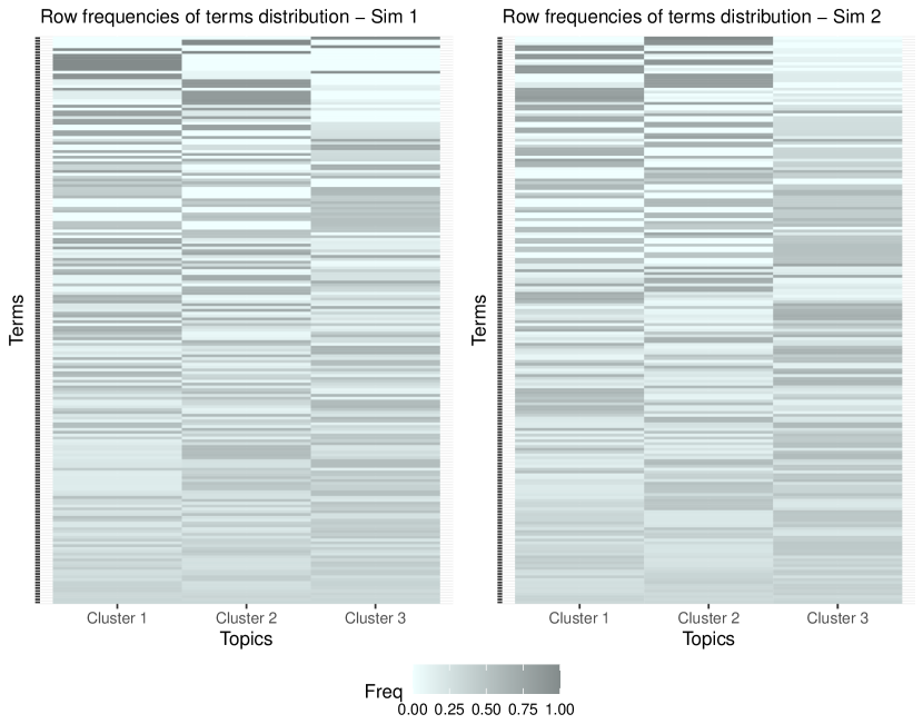
Figure 3: Heatmap of the conditional distribution of features across the classes. The left panel refers to the first simulation study and the right panel to the second ones.

Clustering performance has been measured by using both the Adjusted Rand Index (ARI) and the accuracy rate. The former is a corrected-for-chance version of the Rand Index (Hubert and Arabie, 1985), that measures the degree to which two partition of objects agree; Romano et al. (2016) proved that this measure is particularly indicated in presence of large equal sized reference clusters. The latter is defined as the ones’complement of the misclassification error rate. Table 1 shows the Adjusted Rand Index and the accuracy obtained by a deep MoU model for different values of $k_{2}$, ranging from 1 to 5. We run an MCMC chain with 5000 iterations, discarding the first 2000 as burn-in. Visual inspection assured that this burn-in was largely sufficient.

Table 1: Simulated Data, simulation study 1. Adjusted Rand Index (ARI) and Accuracy of Deep MoU for $k_{1}=3$ and different values of $k_{2}$.

$k_{2}$	ARI	Accuracy
1	0.468	0.755
2	0.940	0.980
3	0.910	0.970
4	0.934	0.980
5	0.925	0.975

Table 2: Simulated Data, simulation study 2. Adjusted Rand Index (ARI) and Accuracy of Deep MoU for $k_{1}=3$ and different values of $k_{2}$.

$k_{2}$	ARI	Accuracy
1	0.824	0.940
2	0.811	0.935
3	0.798	0.930
4	0.811	0.935
5	0.797	0.930

The results show how the model with $k_{2}>1$ is really effective in clustering the data and, as desirable, the model with $k_{2}=2$ (i.e. the setting that reflects the generative process of the data) resulted to be the best one in terms of recovering the ‘true’ grouping structure. The gap between $k_{2}=1$ and $k_{2}>1$ is relevant, however the performance remains elevate for the various $k_{2}>1$, thus indicating that a deep structure can be really effective in clustering such kind of data.

In a second simulation study we tested the performance of a deep MoU with data that are not originated according to a deep generative process, but simply by $k_{1}=3$ balanced groups, $T=n=200$ and $N_{d}=20$, $\forall d$. Panel (b) of Figure 3 displays the row frequency distributions of the generated features. As shown in Table 2, in this situation, the deep model with $k_{2}>1$ does not significantly improve the clustering performance, and the accuracy remains stable as $k_{2}$ increases. This suggests that when the data are pretty simple, and are not high-dimensional, a deep algorithm is not more efficient than the conventional MoU.

The third simulation study aimed at measuring the accuracy of the estimated parameters $\bm{\alpha}$ and $\bm{\beta}$ in data with double structure $k_{1}=3$ and $k_{2}=2$, allowing for different combinations of $T$, $n$ and $N$, so as to measure the effect of data dimensionality and level of sparsity on the goodness of fit. We considered a total of 8 different scenarios generated according to the combinations of $T=\{100,200\}$, $n=\{100,200\}$ and $N=\{10,20\}$. Table 3 contains the Euclidean distance between the true parameter vectors and the posterior means, normalized over $T$.

Table 3: Simulated Data, simulation study 3. Precision of the estimated parameters for different values of $n$, $T$ and $N$.

n	T	N	$\frac{||\bm{\beta}_{1}-\hat{\bm{\beta}_{1}}||}{T}$	$\frac{||\bm{\beta}_{2}-\hat{\bm{\beta}_{2}}||}{T}$	$\frac{||\bm{\beta}_{3}-\hat{\bm{\beta}_{3}}||}{T}$	$\frac{||\bm{\alpha}_{1}-\hat{\bm{\alpha}_{1}}||}{T}$	$\frac{||\bm{\alpha}_{2}-\hat{\bm{\alpha}_{2}}||}{T}$
100	100	10	5.016	5.357	4.737	0.488	0.596
100	200	10	5.360	5.754	5.455	0.511	0.516
100	100	20	3.983	3.917	3.166	0.340	0.329
100	200	20	5.396	4.261	4.220	0.375	0.392
200	100	10	3.999	4.188	5.061	0.317	0.370
200	200	10	4.630	4.540	5.934	0.439	0.441
200	100	20	3.275	5.488	3.205	0.261	0.291
200	200	20	3.912	3.435	3.982	0.311	0.315

As expectable, for a given $T$ the goodness of fit improves as the number of documents increases. The level of sparsity has a relevant role as well: when $N$ increases the documents are more informative and the parameter estimates become more accurate.

5.1 Application to real data

The effectiveness of the proposed model is demonstrated by using four textual datasets, including the introduced ticket data. We compare the Deep MoU with conventional clustering strategies: $k$-means (Lloyd, 1982) with cosine distance ($k$-means) and with Euclidean distance on data transformed according to Semantic Analysis (LSA $k$-means), Partition Around Medoids (PAM, Kaufman and Rousseeuw, 2009), Mixture of Gaussians on semantic-based transformed data (MoG, McLachlan and Peel, 2000), Hierarchical clustering according to Ward’s method (HC, Murtagh and Legendre, 2014) with cosine dissimilarity, Latent Dirichlet Allocation (LDA, Blei et al., 2003), Mixtures of Unigrams (MoU, Nigam et al., 2000) estimated via the EM algorithm (Dempster et al., 1977), spectral clustering (SpeCl, Ng et al., 2002) and affinity propagation clustering (AffPr, Frey and Dueck, 2007) with normalized linear kernel.

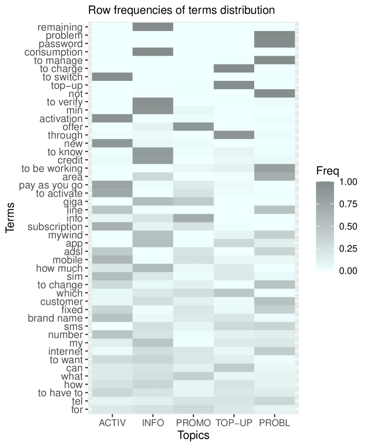
Figure 4: Heatmap of the conditional distribution of terms across classes. The shades reflect the distribution of row frequencies

The CNAE-9 dataset contains 1080 documents of free text business descriptions of Brazilian companies categorized into 9 balanced categories (Ciarelli and Oliveira, 2009; Ciarelli et al., 2010) for a total of 856 pre-processed words. Since the classes 4 and 9 are the most overlapped we considered also the reduced CNAE-2 dataset composed by these two groups only which consists of 240 documents and 357 words. This data set is highly sparse: the 99.22% of the document-term matrix entries are zeros.

The BBC dataset consists of 737 documents from the BBC Sport website corresponding to sport news articles in five topics/areas (athletics, cricket, football, rugby, tennis) from 2004-2005 (Greene and Cunningham, 2006). After a preprocessing phase aimed at discarding non-relevant words, the total number of features is 1075. This dataset is moderately sparse with a fraction of zeros equal to 92.36%.

The ticket dataset contains $n=2129$ tickets and $T=489$ terms obtained after preprocessing: original raw data were processed via stemming, so as to reduce inflected or derived words to their unique word stem, and some terms have been filtered out in order to remove very common non-informative stopwords words in the Italian language. The tickets have then been classified by independent operators to $k=5$ main classes described in Table 4.

Table 4: Real Data. Number of tickets for each class.

Class	Description	Freq.
ACTIV	Activation of SIM, ADSL, new contracts	407
INFO	General information about current balance, consumption, etc.	471
PROMO	Request of information about new offers and promotions	376
TOP-UP	Top-up	435
PROBL	Problems with password, top-up, internet connection, etc.	440

The peculiarity and major challenge of this dataset is the limited number of words used, on average, for each ticket. In fact, after preprocessing, the tickets have an average length of 5 words. A graphical representation of the data, after the preprocessing step, is shown in Figure 4. The heatmap shows the row frequency distributions of the most common terms (overall occurrences $\geq$ 50). As clear from the shades, each class is characterized by a limited set of specific words, while the majority is uniformly distributed across them, thus making the classification problem particularly challenging. In order to have further details about the terms characterizing the tickets within each topic, Figure 5 displays the most frequent words.

Data are characterized by a large amount of sparsity with the 99.05% of zeros: as a consequence, most conventional clustering strategies fail.

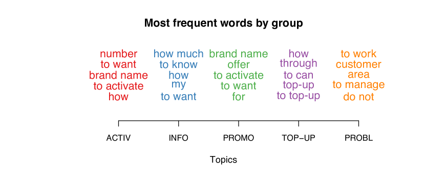
Figure 5: Most frequent terms within each group

Tables 5 and 6 show, respectively, the accuracy and the ARI of the different methods on the presented data sets. For comparative reasons, the true number of clusters was considered as known for all the methods.

Table 5: Real Data. Accuracy (multiplied by 100) for different methods.

Method	CNAE-2	CNAE-9	BBC	Ticket
$k$-means	55.8	59.8	76.5	51.6
LSA $k$-means	65.0	54.4	40.6	46.4
PAM	52.5	11.9	28.8	22.2
MoG	50.4	37.6	43.6	43.8
HC	51.2	13.2	25.4	22.5
LDA	53.3	64.6	41.0	31.8
MoU	60.8	69.6	59.0	74.3
SpeCl	72.9	50.3	44.5	53.0
AffPr	59.2	58.9	53.5	51.7

Table 6: Real Data. Adjusted Rand Index (ARI) for different methods.

Method	CNAE-2	CNAE-9	BBC	Ticket
$k$-means	-0.010	-0.418	-0.567	-0.233
LSA $k$-means	-0.088	-0.282	-0.038	-0.135
PAM	-0.002	-0.000	-0.031	-0.000
MoG	-0.000	-0.092	-0.060	-0.158
HC	-0.003	-0.005	-0.004	-0.001
LDA	-0.000	-0.507	-0.092	-0.000
MoU	-0.043	-0.562	-0.226	-0.523
SpeCl	-0.207	-0.284	-0.104	-0.224
AffPr	-0.030	-0.338	-0.189	-0.219

Among the considered methods, spectral clustering, $k$-means and mixtures of Unigrams are the most effective method for classifying the datasets. An advantage of MoU, which is inherited by the proposed Deep MoU, is that it seems to be not affected by the large number of zeros like the other methods, as it is based on proportions. The Latent Dirichlet Allocation model, despite its flexibility, is not able to improve the classification on these short documents, because it is based on the assumption of multiple-topics for each document, which is not realistic for short data, as in the case of ticket dataset.

We applied Deep MoU with $k_{2}=1,\ldots,5$. For each setting we run 5000 iterations of the MCMC algorithm, discarding the first 2000 as burn-in. From graphical visualization and diagnostic criteria we observed convergence and stability to the different choices of starting points and hyperparameters $\delta$, so we considered $\delta=1$.

Tables 7 and 8 contain the clustering results of the Deep MoU on the datasets, measured by accuracy and ARI respectively. The case $k_{2}=1$ corresponds to a Bayesian MoU and classification is improved with respect to the conventional MoU in most all empirical cases. A probable reason for that is the adoption of Dirichlet-Multinomials (in Bayesian MoU) instead of classical Multinomials (in frequentist MoU), which are more flexible in modeling overdispersion with respect to the multinomial framework (Wilson and Koehler, 1991). In our analysis, the only exception is represented by the dataset CNAE-9, which is particularly challenging because it is composed by 9 unbalanced groups. In this case, classical MoU perform slightly better in terms of misclassification rate and ARI. This may depend on a particularly good starting point of the EM-algorithm for fitting MoU, which is initialized by the $k$-means clustering.

When we move from $k_{2}=1$ to a deeper structure with $k_{2}=2$ or $k_{2}=3$ the accuracy improves in all the analyzed experiments. This proves how the introduction of the parameters $\bm{\alpha}_{j}$ may be beneficial for classification. When the hidden nodes are greater than 3 ($k_{2}=4$ or $k_{2}=5$) results seem to be little worsened, probably because of the larger number of parameters to be estimated.

Table 7: Real Data. Accuracy (multiplied by 100) of Deep MoU for different number of nodes $k_{2}$.

$k_{2}$	CNAE-2	CNAE-9	BBC	Ticket
1	81.2	50.1	95.5	76.2
2	93.3	73.3	95.8	89.2
3	92.9	77.5	95.9	87.6
4	92.5	77.3	93.9	85.6
5	91.2	76.4	93.9	83.3

Table 8: Real Data. Adjusted Rand Index (ARI) of Deep MoU for different number of nodes $k_{2}$.

$k_{2}$	CNAE-2	CNAE-9	BBC	Ticket
1	0.388	0.290	0.888	0.616
2	0.750	0.667	0.894	0.757
3	0.736	0.661	0.895	0.721
4	0.721	0.663	0.848	0.681
5	0.679	0.615	0.843	0.651

6 Final Remarks

In this paper we have proposed a deep learning strategy that extends the Mixtures of Unigrams model. With respect to other clustering methods, MoUs have desirable features for textual data. Firstly, document-term matrices usually contain the frequencies of the words in each document; for this reason, MoUs represent an intuitive choice, since they are based on multinomial distributions that are the probabilistic distributions for modeling positive frequencies. Moreover, as MoUs naturally model proportions, they are not affected by the large amount of zeros of the datasets like other methods, so they are a proper choice for modeling very short texts and sparse datasets. Furthermore, MoU are based on the idea that documents related to the same topic have similar distributions of terms, which is realistic in practice. Taking a mixture of $k$ multinomials means doing clustering into $k$ topics/groups: there is a unique association between documents and topics.

All these nice characteristic are inherited by the proposed Deep MoU model. The proposed Deep MoU is particularly effective in clustering with challenging issues (sparsity, short document length and high-dimensionality). Being hierarchical in its nature, the model can be easily estimated by a MCMC algorithm in a Bayesian framework. In our analysis we chose non-informative priors, because there is little prior information available on the empirical context. The estimation algorithm produces good results in all the simulated and real situations considered here.

The proposed model could be extended in several directions: as discussed in Section 3, several hidden layers (instead of just a single one) could be considered. The merging function $\bm{\beta}_{i}(1+\bm{\alpha}_{j})$ has been defined for identifiability reasons under the idea that the number of estimated groups is $k_{1}$ and the latent layer is only aimed at perturbing the $\bm{\beta}_{i}$ parameters for capturing some residual heterogeneity inside the groups. Of course, more complex nonlinear functions could be considered, without however losing sight of identifiability. In case of non-extreme sparsity and long documents, the model could be also extended to allow for deep m-gram models. We leave all these ideas to future research.

References

- Baek et al. (2010) Baek, J., G. McLachlan, and L. Flack (2010). Mixtures of factor analyzers with common factor loadings: applications to the clustering and visualization of high-dimensional data. IEEE Trans Pattern Anal Mach Intell. 32(7), 1298 – 1309.
- Blei et al. (2003) Blei, D. M., A. Y. Ng, and M. I. Jordan (2003). Latent dirichlet allocation. Journal of machine Learning research 3(Jan), 993–1022.
- Ciarelli and Oliveira (2009) Ciarelli, P. M. and E. Oliveira (2009). Agglomeration and elimination of terms for dimensionality reduction. In Proceedings of the 2009 Ninth International Conference on Intelligent Systems Design and Applications, ISDA ’09, Washington, DC, USA, pp. 547–552. IEEE Computer Society.
- Ciarelli et al. (2010) Ciarelli, P. M., E. O. T. Salles, and E. Oliveira (2010). An evolving system based on probabilistic neural network. In 2010 Eleventh Brazilian Symposium on Neural Networks, pp. 182–187.
- Dempster et al. (1977) Dempster, A. P., N. M. Laird, and D. B. Rubin (1977). Maximum Likelihood from Incomplete Data via the EM Algorithm. Journal of the Royal Statistical Society. Series B (Methodological) 39(1), 1–38.
- Fraley and Raftery (2002) Fraley, C. and A. Raftery (2002). Model-based clustering, discriminant analysis and density estimation. Journal of the American Statistical Association 97, 611–631.
- Frey and Dueck (2007) Frey, B. J. and D. Dueck (2007). Clustering by passing messages between data points. Science 315(5814), 972–976.
- Greene and Cunningham (2006) Greene, D. and P. Cunningham (2006). Practical solutions to the problem of diagonal dominance in kernel document clustering. In Proc. 23rd International Conference on Machine learning (ICML’06), pp. 377–384. ACM Press.
- Griffiths and Steyvers (2004) Griffiths, T. L. and M. Steyvers (2004). Finding scientific topics. Proceedings of the National Academy of Sciences 101(suppl 1), 5228–5235.
- Hubert and Arabie (1985) Hubert, L. and P. Arabie (1985). Comparing partitions. Journal of classification 2(1), 193–218.
- Kaufman and Rousseeuw (2009) Kaufman, L. and P. J. Rousseeuw (2009). Finding groups in data: an introduction to cluster analysis, Volume 344. John Wiley & Sons.
- LeCun et al. (2015) LeCun, Y., Y. Bengio, and G. Hinton (2015). Deep learning. Nature 521(7553), 436–444.
- Li (2005) Li, J. (2005). Clustering based on a multilayer mixture model. Journal of Computational and Graphical Statistics 14(3), 547–568.
- Lloyd (1982) Lloyd, S. (1982). Least squares quantization in pcm. IEEE transactions on information theory 28(2), 129–137.
- McLachlan et al. (2003) McLachlan, G., D. Peel, and R. Bean (2003). Modelling high-dimensional data by mixtures of factor analyzers. Computational Statistics & Data Analysis 41(3), 379 – 388.
- McLachlan and Peel (2000) McLachlan, G. J. and D. Peel (2000). Finite Mixture Models. Wiley.
- Montanari and Viroli (2010) Montanari, A. and C. Viroli (2010). Heteroscedastic factor mixture analysis. Statistical Modelling 10(4), 441–460.
- Murtagh and Legendre (2014) Murtagh, F. and P. Legendre (2014). Ward’s hierarchical agglomerative clustering method: which algorithms implement ward’s criterion? Journal of classification 31(3), 274–295.
- Ng et al. (2002) Ng, A. Y., M. I. Jordan, and Y. Weiss (2002). On spectral clustering: Analysis and an algorithm. In Advances in neural information processing systems, pp. 849–856.
- Nigam et al. (2000) Nigam, K., A. McCallum, S. Thrun, and T. Mitchell (2000). Text classification from labeled and unlabeled documents using EM. Machine learning 39, 103–134.
- Peng et al. (2018) Peng, X., J. Feng, S. Xiao, W.-Y. Yau, J. T. Zhou, and S. Yang (2018). Structured autoencoders for subspace clustering. IEEE Transactions on Image Processing 27(10), 5076–5086.
- Peng et al. (2016) Peng, X., Z. Yu, Z. Yi, and H. Tang (2016). Constructing the l2-graph for robust subspace learning and subspace clustering. IEEE transactions on cybernetics 47(4), 1053–1066.
- Romano et al. (2016) Romano, S., N. X. Vinh, J. Bailey, and K. Verspoor (2016). Adjusting for chance clustering comparison measures. The Journal of Machine Learning Research 17(1), 4635–4666.
- Schmidhuber (2015) Schmidhuber, J. (2015). Deep learning in neural networks: An overview. Neural Networks 61, 85–117.
- Tang et al. (2012) Tang, Y., G. E. Hinton, and R. Salakhutdinov (2012). Deep mixtures of factor analysers. In J. Langford and J. Pineau (Eds.), Proceedings of the 29th International Conference on Machine Learning (ICML-12), pp. 505–512. New York, NY, USA: ACM.
- Tomović et al. (2006) Tomović, A., P. Janičić, and V. Kešelj (2006). n-gram-based classification and unsupervised hierarchical clustering of genome sequences. Computer methods and programs in biomedicine 81(2), 137–153.
- van den Oord and Schrauwen (2014) van den Oord, A. and B. Schrauwen (2014). Factoring variations in natural images with deep gaussian mixture models. In Z. Ghahramani, M. Welling, C. Cortes, N. D. Lawrence, and K. Q. Weinberger (Eds.), Advances in Neural Information Processing Systems 27, pp. 3518–3526. Curran Associates, Inc.
- Viroli (2010) Viroli, C. (2010). Dimensionally reduced model-based clustering through mixtures of factor mixture analyzers. Journal of Classification 27(3), 363–388.
- Viroli and McLachlan (2019) Viroli, C. and G. J. McLachlan (2019, Jan). Deep Gaussian mixture models. Statistics and Computing 29(1), 43–51.
- Wilson and Koehler (1991) Wilson, J. and K. Koehler (1991). Hierarchical models for cross-classified overdispersed multinomial data. Journal of Business and Economic Statistics 9(1), 103–110.
- Zhou et al. (2018) Zhou, J. T., H. Zhao, X. Peng, M. Fang, Z. Qin, and R. S. M. Goh (2018). Transfer hashing: From shallow to deep. IEEE transactions on neural networks and learning systems 29(12), 6191–6201.