Correlation Patterns in Foreign Exchange Markets

Abstract

The value of an asset in a financial market is given in terms of another asset known as numeraire. The dynamics of the value is non-stationary and hence, to quantify the relationships between different assets, one requires convenient measures such as the means and covariances of the respective log returns. Here, we develop transformation equations for these means and covariances when one changes the numeraire. The results are verified by a thorough empirical analysis capturing the dynamics of numerous assets in a foreign exchange market. We show that the partial correlations between pairs of assets are invariant under the change of the numeraire. This observable quantifies the relationship between two assets, while the influence of the rest is removed. As such the partial correlations uncover intriguing observations which may not be easily noticed in the ordinary correlation analysis.

Keywords First keyword  $\cdot$ Second keyword  $\cdot$ More

1 Introduction

Financial markets‘ data has traditionally challenged economists, mathematicians, and statisticians. However, in recent years, physicists have joined in providing answers on different features of these data which resulted in the emergent field of econophysics [1].

A particularly interesting feature of financial markets data is the, not yet fully explored, complex interdependent dynamics of the prices between various assets, which is most often modeled through the empirical correlations. This issue has been of specific value to the econophysics community and its members have provided numerous contributions addressing the relationships between stocks, market indexes and currencies [2, 3, 4, 5, 6, 7, 8, 9, 10].

In a foreign exchange market, the pairwise correlations between assets constitute a matrix. To understand the significant relationships in this matrix, one usually constructs a network by linking the strongly correlated pairs. The pairs are usually chosen via standard algorithms, such as Minimum Spanning Tree (MST) [2] or Planar Maximally Filtered Graph (PMFG) [11, 12]. It has been acknowledged that the correlation matrix and hence the networks generated by MST and PMFG, in general depend on the choice of the base asset, formally known as numeraire, used to measure the value of all other assets. Moreover, changing the numeraire may also distort the plausibility of several economic theories. For instance, the key theory of exchange rates, the Purchasing Power Parity, relies on numeraire invariance, i.e., different numeraires should yield same conclusions. However, a growing body of literature negates the empirical validity of this property in foreign exchange markets [13, 14, 15]. In spite of these observations, the exact implications created by substituting the numeraire for another asset are yet to be determined.

Relating variables measured in different reference frames has a long history in physics. For example, the famous Galilean [16] and Lorentz [17] transformations are used for establishing correspondences between kinematic variables in classical and relativistic scenarios, respectively. Evidently, the role of reference frame in finance is played by the numeraire. In stock markets the natural choice of numeraire is the domestic currency, whereas at a foreign exchange different assets may fit for this purpose. In studies examining the properties of the latter markets, usually the most traded asset is taken as numeraire, while another less liquid asset is used to compare the results [6, 8].

Motivated by these observations, here we derive the transformation equations for the key statistical quantities (means and covariances) when the numeraire is changed. As an application of these transformations, we discuss the choice of numeraire used for valuing the performance of a portfolio of assets, and provide arguments that the most appropriate numeraire is the local currency of the investor. More importantly, we give a thorough empirical analysis which not only confirms our findings, but also provides a detailed overview on the influence of the numeraire choice on the resulting correlations. In particular, we show that there is a typical pattern where certain correlations which are significant in one numeraire become insignificant in another.

Finally, we also comment on a numeraire invariant measure for capturing the correlation between assets. In fact, we find that one such measure is the partial correlation – the quantification of the linear relationship between two assets while controlling for the potential effect of all other assets in the market. As such, a network constructed via the partial correlations may provide a more adequate illustration on the pairwise relationships in a foreign exchange market.

The rest of the paper is organized as follows. In Section 2 we begin by providing the theoretical background and analysis of the problem of numeraire change. Section 3 describes the data used for empirical verification of the developed theory. In Section 4 we present the empirical results and discuss the implications created by substituting the numeraire. Finally, Section 5 summarizes our findings.

2 Theoretical analysis

The dynamics of exchange rates is in general non-stationary, and hence non-ergodic. This implies that one cannot exploit the raw values to examine the relationships between different assets. A convenient way to circumvent this problem is to instead focus on the logarithmic returns of exchange rates, which are known for their stationary dynamics [18].

We assume that the distribution of these log returns is multivariate Gaussian, which is a plausible assumption under the efficient market hypothesis [19], even though there are observations suggesting otherwise [20, 21, 22]. It is widely known that the Gaussian distribution is fully defined by its mean and covariance structure, which in turn is dependent on the chosen numeraire. This is of particular relevance in a foreign exchange market, as in it the value of any asset is given as a ratio with respect to another asset, i.e. the exchange rate. Thus, there is no single value of an asset, but many relative prices expressed in terms of the other assets. Once one selects a numeraire, even a random one, and hence determines the value of some asset in the market, in absence of arbitrage the values of the remaining ones are also determined. This is analogous to the assignment of a voltage to some node, which uniquely determines the voltages of all other nodes in an electrical circuit. In the following we analytically evaluate the consequences of changing numeraire on the values of the means, covariances and correlations in an arbitrary foreign exchange market.

2.1 Mean and covariance transformations

We begin by assuming that the observations arrive discretely at moments $1,2,\dots$, and randomly assign values to one of the currencies $U_{1},U_{2},\dots$. The values of the remaining currencies are then determined from the existing exchange rates. This indicates that the log return $x^{u}$ of any currency $X$ given in the numeraire $U$ at a particular moment $n$ would be

$$x^{u}=\log\left(\frac{X_{n}}{U_{n}}\right)-\log\left(\frac{X_{n-1}}{U_{n-1}}\right).$$ (1)

The return $x^{w}$ of $X$ in another numeraire $W$ is simple linear combination of the returns

$$x^{w}=\log\left(\frac{X_{n}}{U_{n}}\frac{U_{n}}{W_{n}}\right)-\log\left(\frac{X_{n-1}}{U_{n-1}}\frac{U_{n-1}}{W_{n-1}}\right)=x^{u}-w^{u}.$$ (2)

Since we are working with ergodic observables, we can apply the averaging rules, and conclude that the change of numeraire results in linear transformation of the mean of log returns as well,

$$\langle x^{w}\rangle=\langle x^{u}\rangle-\langle w^{u}\rangle,$$ (3)

where the brackets denote averages. The covariance between the log returns of currencies $X$ and $Y$ in the first numeraire $U$ is defined as

$$C_{x,y}^{u}=\langle(x^{u}-\langle x^{u}\rangle)(y^{u}-\langle y^{u}\rangle)\rangle.$$ (4)

By using the return transformations (2) in the definition of the covariance (4), after simple algebra one can easily show that the covariance in the second base is

$$C_{x,y}^{w}=C_{x,y}^{u}-C_{x,w}^{u}-C_{y,w}^{u}+C_{w,w}^{u}.$$ (5)

The last expression is transformation of the covariance from one numeraire to another, and resembles those used in kinematics. Furthermore, from (5) we can directly extract the Pearson correlation coefficient, $r^{w}_{x,y}=C^{w}_{x,y}/\sqrt{C^{w}_{x,x}C^{w}_{y,y}}$, as

$$r_{x,y}^{w}=\frac{C_{x,y}^{u}-C_{x,w}^{u}-C_{y,w}^{u}+C_{w,w}^{u}}{\sqrt{\left(C_{x,x}^{u}-2C_{x,w}^{u}+C_{w,w}^{u}\right)\left(C_{y,y}^{u}-2C_{y,w}^{u}+C_{w,w}^{u}\right)}}.$$ (6)

We note that a special case of the relationship (5) is the variance transform $C_{x,x}^{w}=C_{x,x}^{u}-2C_{x,w}^{u}+C_{w,w}^{u}$, which has relevance in calculation of covariances when the three necessary variances are known [23, 24]. This relationship is widely used in determining the covariance between two assets from the corresponding values of their implied variances, which in turn are estimated from the respective option prices [25, 26].

2.2 Variance of portfolio

Modern portfolio theory states that the optimal portfolio is achieved by diversifying investments in a combination which leads to the lowest variance for given mean. It is evident that, in this aspect, changing the numeraire also modifies the parameter values of the portfolio – its expected return and variance. To find the respective transformation that is needed when one changes the numeraire, we consider a portfolio of assets, $X_{1},X_{2},,\ldots,X_{N}$, which under base $U$ has value $X^{u}=\sum_{i=1}^{N}\alpha_{i}(X_{i}/U)$, where $\alpha_{i}$ is the share of investments in $X_{i}$. Consequently, its return in units of $U$ is

$$x^{u}=\sum_{i=1}^{N}\alpha_{i}x_{i}^{u}.$$ (7)

The portfolio return changes in the same manner as in equation (1), and its value in the numeraire $W$ is

$$x^{w}=\sum_{i=1}^{N}\alpha_{i}(x_{i}^{u}-w^{u})=x^{u}-w^{u}.$$ (8)

Going further one can obtain the variance of the portfolio in numeraire $U$ as

$$C_{x,x}^{u}=\sum_{i=1}^{N}\alpha_{i}^{2}C_{x_{i},x_{i}}^{u}+\sum_{i\neq j}\alpha_{i}\alpha_{j}C_{x_{i},x_{j}}^{u}.$$ (9)

After expanding the terms appearing in the transformation of the portfolio return (8) into the definition of the covariance (4) and some rearrangements we find that

$$C_{x,x}^{w}=\sum_{i=1}^{N}\alpha_{i}^{2}C_{x_{i},x_{i}}^{u}+\sum_{\begin{subarray}{c}i,j=1\\ i\neq j\end{subarray}}^{N}\alpha_{i}\alpha_{j}C_{x_{i},x_{j}}^{u}-2\sum_{i=1}^{N}\alpha_{i}C_{x_{i},w}^{u}+C_{w,w}^{u}.$$ (10)

This is compactly written as

$$C_{x,x}^{w}=C_{x,x}^{u}-C_{x,w}^{u}+C_{w,w}^{u},$$ (11)

by defining $C_{x,w}^{u}=2\sum_{i=1}^{N}\alpha_{i}C_{x_{i},w}^{u}$ as the covariance between the portfolio and the second numeraire $W$ observed from the point of view of the first one $U$.

Similarly to the twin paradox in special relativity [27], the dependence of the variance on the base currency poses a dilemma about which numeraire should be used as reference frame. To resolve this issue, let us assume that a particular investor is in a country with currency $U$. In order to finance a portfolio with starting value $X(s)$ the agent should borrow the same amount in currency $U$ from a local bank, and return it later at the final moment $f$, again in the same currency. Furthermore, suppose that the bank interest rate is zero and that the portfolio is valued at one currency unit $U$. Then, the initial and final wealth of the investor are correspondingly $0$ and $X^{u}(f)-U$. The variance of the portfolio is given by equation (9).

The same investor should observe the variance expressed in the numeraire $W$ only if it is initially financed by a credit denominated in that asset. This follows by observing the initial credit $U/W(s)$, as valued in the second asset, and then purchasing the portfolio. In particular, by assuming negligible transaction costs (for simplicity), the value of the portfolio at purchase is

$$X^{w}(s)=\sum_{i=1}^{n}\alpha_{i}\frac{X_{i}(s)}{W(s)}=\sum_{i=1}^{n}\alpha_{i}\frac{X_{i}(s)}{U}\frac{U}{W(s)},$$ (12)

in $W$ currency units, with the same expression holding at the closing time $f$. If one substitutes the final and starting moments $f$ and $s$, with $n$ and $n-1$ respectively, the return on the portfolio is given as in (8), i.e. $x^{w}=x^{u}-u^{w}=x^{u}+w^{u}$. This means that the log return of the investments is in one part due to the portfolio return $x^{u}$ and in another one due to the exchange rate return $w^{u}$ between $W$ and $U$. On the other hand, it is obvious that the return of the borrowing cancels the exchange rate contribution of the return in investments since its value is $-w^{u}$. Consequently, the return on the portfolio and respectively its variance is identical in both cases, which means that it might be more convenient for the investor to use its domestic currency as numeraire.

2.3 Partial correlation

To account for the possibility that other variables drive the relationship between the two variables under study, one calculates the respective partial correlation [10, 28, 29]. For the case of foreign exchange markets, this translates to the correlation between the log return of two assets controlled for the return of all other assets exchanged in the market. To examine the numeraire dependence of this quantity, let us first define the set $\mathbb{R}$ containing all possible returns of all assets in the foreign exchange as valued in every possible numeraire. Then, the partial correlation between the returns of assets $X$ and $Y$ valued in numeraire $U$ reads

$$\rho^{u}_{x,y}=\langle\left(x^{u}-\langle x^{u}\rangle\right)\left(y^{u}-\langle y^{u}\rangle\right)|\mathbb{R}\backslash\{x^{u},y^{u}\}\rangle.$$ (13)

The partial correlation with numeraire $W$ is defined in the same way, only conditioned on $\mathbb{R}\backslash\{x^{w},y^{w}\}$. Notice that the linear transformation between the returns of $x$ in $u$ and $w$, $x^{w}=x^{u}-w^{u}$, contains the constant term $w^{u}$ which is the sets of known variables in consideration of the two partial correlations $\rho^{u}_{x,y}$ and $\rho^{w}_{x,y}$. Combining this fact with the property that adding constants in two variables does not change their correlation, implies that we can write the latter partial correlation as

$$\rho^{w}_{x,y} = \langle\left(x^{w}-\langle x^{w}\rangle\right)\left(y^{w}-\langle y^{w}\rangle\right)|\mathbb{R}\backslash\{x^{w},y^{w}\}\rangle=$$ (14)

$$= \langle\left(x^{u}-w^{u}-\langle x^{u}-w^{u}\rangle\right)\left(y^{u}-w^{u}-\langle y^{u}-w^{u}\rangle\right)|\mathbb{R}\backslash\{x^{u},y^{u}\}\rangle=$$

$$= \langle\left(x^{u}-\langle x^{u}\rangle\right)\left(y^{u}-\langle y^{u}\rangle\right)|\mathbb{R}\backslash\{x^{u},y^{u}\}\rangle.$$

Hence, the partial correlation between the return of two assets controlled for the returns of all other assets traded in the market, is invariant on the numeraire. As a side note, we point out that such partial correlations are easily calculated through the precision matrix $\mathbf{P}$ which is the inverse of the correlation matrix $\mathbf{C}$, and by utilizing the following normalization

$$\rho_{x,y}=-\frac{P_{x,y}}{\sqrt{P_{x,x}P_{y,y}}},$$ (15)

for each pair of assets $X$ and $Y$ [30].

3 Data

To verify the presented findings, we study market data provided by the Pacific Exchange Rate Service Dataset (PERS). PERS is a freely available dataset which provides daily values of 92 currencies and commodities priced in various numeraires. In the analysis, we opted to include commodities because combining them with currencies allows for capturing more general patterns in financial markets. In fact, as we will see later on, there appear direct relations between the currencies and commodities.

As a time frame we utilized the four year period between 2014 and 2017. Since calculation of the log returns requires data for two consecutive days, we excluded from the analysis all data points for which there was no consecutive data. Finally, from the analysis we excluded all currencies for which there were at least ten missing values and those assets that have constant exchange rates with the USD for at least five working days. We note that the considered period, the precious metals present in the dataset have around 30 missing values. Nevertheless, we kept them in the analysis as they may represent a significant driver in the returns of several currencies. Altogether, we ended up with $897$ log returns data for $48$ currencies and $5$ commodities. The names of the assets together with their abbreviations are listed in Table 1.

Table 1: List of abbreviations of the studied assets

Currencies
AED	U.A. Emirates dirham	KRW	Korean won
ARS	Argentine peso	KWD	Kuwaiti dinar
AUD	Australian dollar	LKR	Sri Lankan rupee
BHD	Bahraini dinar	MAD	Moroccan dirham
BRL	Brazilian real	MXN	Mexican peso
CAD	Canadian dollar	MYR	Malaysian ringgit
CHF	Swiss franc	NOK	Norwegian krone
CLP	Chilean peso	NZD	New Zealand dollar
CNY	Chinese renminbi	PEN	Peruvian nuevo sol
COP	Colombian peso	PHP	Philippines peso
CZK	Czech koruna	PLN	Polish zloty
DKK	Danish krone	RUB	Russian ruble
EUR	EURO	SAR	Saudi Arabian riyal
GBP	British pound	SEK	Swedish krona
HKD	Hong Kong dollar	SGD	Singapore dollar
HNL	Honduran lempira	THB	Thailand baht
HRK	Croatian kuna	TND	Tunisian dinar
HUF	Hungarian forint	TRY	Turkish lira
IDR	Indonesian rupiah	TWD	Taiwanese dollar
ILS	Israeli new sheqel	USD	U.S. dollar
INR	Indian rupee	UYU	Uruguayan peso
ISK	Icelandic krona	VND	Vietnamese dong
JMD	Jamaican dollar	XCD	East Caribbean dollar
JPY	Japanese yen	ZAR	South African rand
Commodities
XAG	Silver ounce	XCT	West Texas barrel
XAU	Gold ounce	XPT	Platinum ounce
XCB	Brent Crude barrel

We point out that the initial data was gathered with US dollar (USD) as numeraire. When calculating the asset values in other numeraires we utilized the triangular equivalence, i.e., a rate $X/Y$ was estimated from the known $X/Z$ and $Y/Z$ as $X/Y=(X/Z)/(Y/Z)$. This is a common approach [31], even though small deviations from the real values known as triangular arbitrage, were found on shorter time scales. On longer scales, such as the daily ones, they are negligible [21]. Once all exchange rates were determined, by taking each of the 53 assets as numeraire, we calculated the daily log returns of the remaining 52 assets, and estimated the corresponding covariance and correlation matrices. To test the significance of all terms in the correlation (covariance) matrices we implemented the Bonferroni correction [32, 33]. Under this test, the level of significance is given by dividing the level of significance under single test with the number of elements in the correlation matrix. Accordingly, we took the level of significance to be $0.05/(53\cdot 53)$.

4 Results

4.1 Empirical validation of the transformations

First, we verify the validity of the transformations developed in the previous section. For this purpose, in Fig. 1 we plot heat maps for the empirical correlations between the studied assets as valued in EUR (Fig. 1a) and in USD (Fig. 1b), and their corresponding transformed correlations, from USD to EUR in Fig. 1c and from EUR to USD in Fig. 1d. One can easily notice the striking resemblance between these two types of correlations. In fact, the coefficient of determination, which quantifies the percentage of the variance in the empirical correlations explained with the transformed correlations, states that almost 100 percent of the variance in both the EUR matrix and USD matrix is explained with the transformations. The same conclusion holds for all other empirical correlations and transformation pairs.

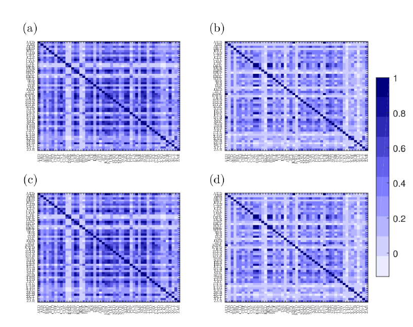
Figure 1: Correlation heat maps. (a) Correlation estimated from data where the numeraire is EUR. (b) Same as (a) only the numeraire is USD (c) Correlations in EUR estimated from transforming the correlation matrix in USD as base currency (d) Same as (c) only the correlations are estimated by transforming the EUR matrix to USD.

4.2 Implications of changing the numeraire

Fig. 1 also reveals the known fact that the numeraire ultimately determines the relationships in the correlation matrix [6, 7, 8]. While one typically uses the correlation matrix to build networks via MST or PMFG, and thus study the leading currencies and the clusters of mutually related assets, here instead we focus on the properties of the correlation matrix. Even though, this is not necessarily the same, we point out that the properties of the correlation matrix are those which uniquely determine the structure of the network.

For this purpose we turn our attention to the correlation matrix as estimated with USD as base currency. In the Appendix in Table LABEL:tab:Corr_USD are shown the correlation coefficients obtained with this currency as numeraire, which are larger than 0.6. In order to extract the more significant ones, we apply filtering by considering only ones that exceed certain threshold.

First, when the threshold is 0.9, one can notice that for this numeraire the strongest positive correlations appear between the currencies of oil exporting Middle Eastern countries, i.e. between AED, KWD and SAR. They are accompanied by a clique of European currencies, CZK, DKK, EUR, and HRK together with the North African MAD. By lowering the threshold to 0.8, HUF and the PLN join the European cluster, while taking an even lower threshold of 0.6, further adds NOK, SEK and TND to the group. At the same time, this results in emergence of an East Asian clique containing the KRW, SGD and TWD, and significance in the correlation between the Oceania pair of AUD and NZD. One can easily hypothesize that the existence of these relations has roots in the geographical proximity of the countries, and hence increased economic interdependence. Without going into further analysis of the other, weaker correlation patterns, we just note that the three major currencies CHF, GBP and JPY in these USD-based calculations are close to the European cluster. The last currency also has very strong correlation with the gold.

If one uses another currency as numeraire, for instance EUR, remarkable differences in the correlation coefficients from those observed in the USD-based calculations are identified. By considering the correlations larger than 0.9, given in the Appendix in Table LABEL:tab:Corr_EUR, one can notice that the Middle East currency trio AED, KWD and SAR is present again. Also a new clique of correlations exceeding 0.9 arises and which consists of CNY, JMD, HKD, LKR and USD. In addition, the correlation between XCD and HKD is also above 0.9. By decreasing the threshold, the later two cliques coalesce, while simultaneously attracting new Asian currencies, in particular, INR, PHP, THB and TWD together with the Latin American PEN, to the cluster. Further lowering the threshold to 0.6 results in inclusion of new members to the big cluster. The new members are the Asian IDR, ILS, KRW, MYR, SGD, and VND, the Latin American currencies CLP and HNL and the CAD. Also, under a lowered threshold one notices the correlation between the Oceania couple AUD and NZD and the joining of MAD to the USD-based mega cluster. It is worth to point out that the MAD was discovered to be rather correlated to the European currencies when observed from the USD as numeraire.

From this correlation analysis one notices that the European cluster appears within USD-based calculations, while the currencies that closely track the dynamics of the US dollar can be detected when EUR is the numeraire. From this observation one could further conjecture a test for determining the strong correlations between two assets $X$ and $Y$ based on two conditions. First, they should be highly correlated in various numeraires, and second, when one of them is used as numeraire (for example $X$), the correlations of the other, $Y$, with the remaining assets should become smaller. Loosely speaking, in base currency $X$ the correlations of $Y$ with the others are masked. If any other currency $Z$ is correlated to both $X$ and $Y$, then the correlation between $X$ and $Y$ in numeraire $Z$, with the other currencies $U$, $r_{y,u}^{z}$ and $r_{x,u}^{z}$, will be small as well. Thus, using the CZK, DKK, or HRK as numeraire produces similar results as EUR – weak correlations of the other currencies from this European group with the rest, while keeping the Middle East and USD clusters of highly correlated currencies. We also found that the masking phenomenon has an effect even on the currencies which could not be easily associated to some cluster. For example, when considered EUR as base currency, the CHF, GBP, and JPY seem to be more correlated to the currencies of the USD cluster, while as seen from the USD perspective they appear closer to the European group.

To confirm the masking phenomenon we also considered using SAR as numeraire, which is the currency of the largest country of the strongly correlated Middle East trio. The respective Pearson correlation coefficients exceeding 0.6 are provided in the Appendix in Table LABEL:tab:Corr_SAR. When filtering the correlations larger than 0.9 one discovers only the European clique, consisting of the CZK, DKK, EUR, HRK and MAD, while a USD-based cluster containing CNY, HKD, JMD, and LKR, appears when the threshold is lowered to 0.8. Again, by considering even weaker correlations, other currencies join to the respective groups, until they merge into one big cluster. For this numeraire we found an interesting exception of the masking phenomenon, i.e., we discovered a high correlation of 0.82 between AED and BHD which was previously missing. This suggests that BHD should belong to a cluster where AED is. As we pointed out previously, such strong correlation should also be observed from other numeraires like the EUR or USD. In fact, the masking should result in weak correlation between AED and BHD when the numeraire is SAR, since, as discovered from the view of the two previous numeraires, SAR is rather closely related to AED. Nevertheless, the results show the opposite. The interpretation behind this finding may be due to the fact both AED and BHD are currencies of oil exporting countries, or due to the economic relations with other countries. In what follows we will offer further indications for the plausibility of the second interpretation, since a very strong but negative partial correlation between SAR and BHD appears. Lastly, we note that using SAR as numeraire pushes the CHF, GBP, and JPY closer to EUR, whereas the previously observed strong correlation of JPY with the gold persists since JPY does not belong to either of the USD and EUR groups.

4.3 Robustness of correlated pairs

As a means to understand the influence of the choice of numeraire on the correlations between other currencies that probably have more independent dynamics, for each asset $X$ we determined the maximal correlation under numeraire $U$, i.e.,

$$r_{x,\max}^{u}=\max_{z}\left\{r_{x,z}^{u}\right\},$$ (16)

by searching for it over all other assets $Z$. The asset $Y$ for which the strongest correlation $r_{x,\max}^{u}$ is obtained can be considered as the most similar to $X$ when the numeraire is $U$. Obviously, this similarity relationship is asymmetrical, and by substituting the numeraire, the most similar asset to $X$ could change as well. In this regard, by taking all numeraires under consideration, for each asset we estimate the number of occurrences of most similar assets. This allows us to effectively reduce the impact of numeraire in determining the similarity and thus develop a robust measure for the significance of the similarity. Clearly, higher number of such occurrences does not imply more pronounced similarity between two assets, as it does not quantify the magnitude of it. It only offers a robust way to identify the asset which most often appears to be “closest” in terms of correlation. Even though, this approach may appear more computationally demanding than the standardly used MST and PMFG, it offers a more comprehensive overview of quantifying the most similar asset as it considers all possible numeraires.

The results can be seen in Table 2 where we report each asset $X$ alongside its most similar asset $Y$ and the number of different numeraires under which $Y$ is most similar to $X$. It can be easily noticed that similar results to the previous discussion regarding the USD, EUR and Middle Eastern cluster hold. Besides this, the performed analysis is able to uncover novel information about the correlation structure. Concretely, here we observe the similarity between Latin American BLR, CLP, COP and MXN, as well as between certain currencies from Asia. From the studied precious metals, the silver and platinum seem to exhibit similar dynamics to that of the gold, while the gold remains most similar to JPY. Moreover, we notice that GBP appears most similar to SGD instead of any other European currency, even when accounting for every possible numeraire from Europe, as compared to the SGD alone. Finally, we remark that HKD and SGD are the two assets which are most similar to the others. While the former currency may appear as a central regional trade unit, due to the fixed exchange rate to the USD, the later has a bigger role in global trading.

Table 2: Most similar assets. The most similar peer (second and fifth column) to certain asset (first and fourth column) is the one which has strongest correlation to the latter in largest number of different numeraires. The number of such occurrences for each pair is given in the third and sixth column.

Asset	Sim. asset	No. occur.	Asset	Sim. asset	No. occur.
AED	SAR	51	MAD	DKK	28
ARS	USD	43	MXN	CLP	29
AUD	NZD	47	MYR	SGD	37
BHD	AED	51	NOK	SEK	46
BRL	MXN	50	NZD	AUD	51
CAD	SGD	36	PEN	HKD	43
CHF	EUR	46	PHP	HKD	38
CLP	COP	17	PLN	HUF	51
CNY	HKD	50	RUB	COP	38
COP	CLP	50	SAR	AED	51
CZK	DKK	51	SEK	EUR	47
DKK	EUR	51	SGD	TWD	47
EUR	DKK	51	THB	HKD	40
GBP	SGD	27	TND	MAD	28
HKD	USD	51	TRY	SGD,ZAR	19
HNL	USD	51	TWD	SGD	44
HRK	DKK	51	USD	HKD	51
HUF	PLN	51	UYU	AED	51
IDR	MYR	31	VND	HKD	50
ILS	SGD	23	XAG	XAU	45
INR	HKD	40	XAU	JPY	43
ISK	DKK	49	XCB	XCT	51
JMD	USD	51	XCD	USD	50
JPY	SGD	30	XCT	XCB	51
KRW	TWD	51	XPT	XAU	50
KWD	AED	50	ZAR	MXN	48
LKR	USD	51

4.4 Network of partial correlations

Using the same data, we estimated the partial correlation between the assets, and as described in the Data section, we used the statistically significant relationships to build a network which describes their relatedness.

The statistically significant partial correlations are given in Table 3, while the resulting network is illustrated in Fig. 2. The network is largely disconnected with only several isolated clusters being formed which can be explained by considering the geographical proximity of countries again. We note that similar findings about the relations between currencies of neighboring countries have been previously obtained with the MST technique [5, 8].

In particular, the largest cluster consists mainly of currencies from South and East Asia. In addition, precious metals can be found in this cluster due to their relation with JPY and THB. Here, it is also noteworthy to point out that the GBP exhibits negative partial correlation with JPY. Another easily interpretable cluster is the group of interconnected European currencies consisting of CZK, DKK, EUR, HRK, ISK and MAD. Interestingly, other European currencies, specifically PLN and HUF, are instead connected to a USD-based cluster due to the negative partial correlation between PLN and USD. This cluster further includes HKD, LKR and JML. The next cluster consists of the Middle east currencies AED, KWD and SAR, which are acompanied with BHD due to its rather strong negative partial correlation with AED.

A rather intriguing cluster centred around MXN appears. This cluster, on the one hand, consists of neighboring Latin American currencies BRL, COP and CLP, and the geographically distant currencies ZAR nad TRY, on the other hand. The last cluster describes the relationships between oiled-based assets, mainly due to the price of West Texas Intermediate being partially correlated with the CAD, whereas the Brent Crude oil is related with RUB. Moreover, the oil production industry is probably the cause for the positive partial correlation between RUB and NOK, which in turn puts the latter with the neighboring SEK into this group, rather than into the EUR-based one. We point out that NOK and SEK have more strong unconditional correlations with the currencies from the other other EU countries than with the RUB. In this cluster the Oceania pair of AUD and NZD is included due to the significant partial correlation between AUD and CAD. Finally, INR and PHP form an isolated pair of mutually influential currencies from neighboring countries.

Table 3: Statistically significant partial correlations.Note that the negative correlations are in bold.

Pair	$\rho_{x,y}$	Pair	$\rho_{x,y}$	Pair	$\rho_{x,y}$
AED/SAR	0.964	CZK/DKK	0.246	AUD/CAD	0.167
HKD/USD	0.936	JPY/SGD	0.245	LKR/USD	0.166
AED/BHD	0.795	IDR/MYR	0.242	JMD/USD	0.165
DKK/EUR	0.640	SGD/TWD	0.225	DKK/ISK	0.164
XCB/XCT	0.495	DKK/MAD	0.223	MXN/TRY	0.161
HUF/PLN	0.446	CLP/COP	0.221	COP/MXN	0.160
AUD/NZD	0.434	MYR/SGD	0.211	AED/KWD	0.145
DKK/HRK	0.434	CZK/HRK	0.208	INR/PHP	0.143
KRW/TWD	0.403	MXN/ZAR	0.203	BRL/MXN	0.139
JPY/XAU	0.362	TRY/ZAR	0.203	THB/XAU	0.139
XAU/XPT	0.347	KRW/SGD	0.192	GBP/JPY	-0.144
XAG/XAU	0.338	NOK/RUB	0.179	PLN/USD	-0.147
NOK/SEK	0.313	RUB/XCB	0.177	BHD/SAR	-0.807
XAG/XPT	0.280	CAD/XCT	0.174

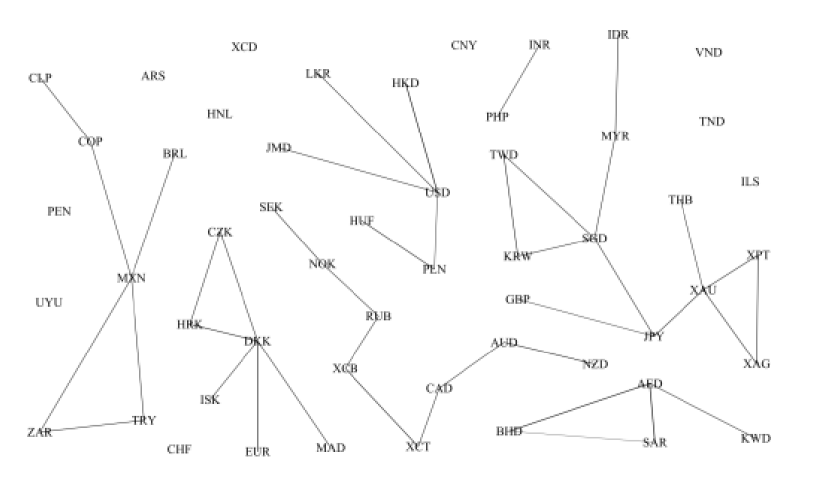
Figure 2: Partial correlation network. The edges represent statistically significant partial correlations.

5 Conclusions

In short summary, in this paper we investigated how the means, covariances and correlations of the logarithmic returns of assets are modified when the numeraire in a foreign exchange is changed. We also showed that the same techniques can be applied for the portfolio of an investor, and thus identify the most appropriate numeraire for him/her to use. This turned out to be the domestic currency of the investor. Finally, we showed that while the magnitude of the ordinary correlations are highly dependent on the choice of numeraire, the partial correlations are invariant in this aspect. The empirial analysis easily confirmed these findings.

Appendix

Table 4: Correlation coefficients larger than 0.6 when the numeraire is USD

Pair	$r_{x,y}$	Pair	$r_{x,y}$	Pair	$r_{x,y}$	Pair	$r_{x,y}$
AED/SAR	0.985	CZK/PLN	0.836	EUR/ISK	0.761	NZD/SGD	0.644
DKK/EUR	0.980	CZK/HUF	0.834	HRK/SEK	0.758	NOK/PLN	0.639
DKK/HRK	0.974	DKK/PLN	0.834	CZK/SEK	0.755	EUR/NOK	0.635
CZK/DKK	0.958	HRK/HUF	0.828	ISK/MAD	0.746	SGD/THB	0.633
EUR/HRK	0.957	HRK/PLN	0.825	KRW/SGD	0.737	AUD/CAD	0.632
CZK/HRK	0.948	EUR/HUF	0.823	AUD/NZD	0.732	DKK/NOK	0.627
CZK/EUR	0.938	EUR/PLN	0.818	MAD/SEK	0.722	HUF/NOK	0.627
DKK/MAD	0.933	DKK/ISK	0.790	SGD/TWD	0.721	CZK/NOK	0.624
EUR/MAD	0.919	MAD/PLN	0.789	HUF/SEK	0.695	ISK/SEK	0.621
AED/KWD	0.918	HUF/MAD	0.789	ISK/PLN	0.693	HRK/NOK	0.620
HRK/MAD	0.915	EUR/SEK	0.783	NOK/SEK	0.692	HRK/TND	0.613
KWD/SAR	0.908	HRK/ISK	0.781	PLN/SEK	0.689	DKK/TND	0.611
CZK/MAD	0.905	CZK/ISK	0.780	HUF/ISK	0.686	EUR/TND	0.608
HUF/PLN	0.866	DKK/SEK	0.776	AUD/SGD	0.668
DKK/HUF	0.837	KRW/TWD	0.767	XCB/XCT	0.647

Table 5: Correlation coefficients larger than 0.6 when the numeraire is EUR

Pair	$r_{x,y}$	Pair	$r_{x,y}$	Pair	$r_{x,y}$	Pair	$r_{x,y}$
HKD/USD	0.998	PEN/THB	0.804	KWD/THB	0.726	ILS/JMD	0.647
AED/SAR	0.995	AED/JMD	0.802	CNY/HNL	0.725	ILS/SGD	0.646
AED/KWD	0.970	JMD/SAR	0.802	AED/PHP	0.724	IDR/JMD	0.646
KWD/SAR	0.967	PEN/PHP	0.800	PHP/SAR	0.722	CAD/THB	0.645
LKR/USD	0.954	KRW/TWD	0.800	AUD/NZD	0.720	ILS/THB	0.645
HKD/LKR	0.952	THB/XCD	0.798	INR/MYR	0.718	AED/HNL	0.644
JMD/USD	0.949	INR/SGD	0.796	HKD/MYR	0.717	MAD/TWD	0.644
CNY/HKD	0.948	MAD/USD	0.795	MYR/USD	0.711	IDR/LKR	0.644
HKD/JMD	0.947	CNY/SGD	0.795	MAD/THB	0.707	HNL/SAR	0.642
CNY/USD	0.946	HKD/MAD	0.794	KWD/PEN	0.706	COP/MXN	0.642
JMD/LKR	0.907	INR/PEN	0.793	CAD/SGD	0.706	ILS/PHP	0.640
USD/XCD	0.906	KWD/USD	0.793	INR/KWD	0.706	CLP/PHP	0.640
HKD/XCD	0.905	HKD/KWD	0.793	SAR/TWD	0.703	AED/MYR	0.638
CNY/LKR	0.905	AED/LKR	0.792	SGD/XCD	0.703	ILS/LKR	0.638
CNY/JMD	0.902	LKR/SAR	0.790	AED/TWD	0.703	KRW/MYR	0.636
HKD/THB	0.881	PEN/TWD	0.781	SAR/SGD	0.693	MYR/SAR	0.636
SGD/TWD	0.881	KRW/SGD	0.781	AED/SGD	0.693	CAD/PEN	0.636
THB/USD	0.878	HKD/SGD	0.780	MAD/PHP	0.691	HKD/VND	0.635
JMD/XCD	0.875	JMD/TWD	0.778	HNL/XCD	0.690	CAD/PHP	0.635
LKR/XCD	0.869	PEN/XCD	0.776	LKR/MYR	0.689	USD/VND	0.635
CNY/THB	0.868	SGD/USD	0.773	KWD/PHP	0.689	IDR/SGD	0.634
CNY/XCD	0.863	LKR/TWD	0.773	JMD/MYR	0.686	ILS/TWD	0.632
HKD/PHP	0.862	MYR/SGD	0.771	MYR/PEN	0.685	CAD/INR	0.632
HKD/PEN	0.859	AED/XCD	0.770	KRW/THB	0.683	KWD/MAD	0.631
PHP/USD	0.858	SAR/XCD	0.770	IDR/MYR	0.682	IDR/TWD	0.631
PEN/USD	0.857	JMD/KWD	0.767	MAD/PEN	0.679	HNL/PHP	0.629
THB/TWD	0.855	PHP/XCD	0.767	KRW/PHP	0.677	AED/CAD	0.628
PHP/THB	0.852	CNY/KWD	0.765	CLP/TWD	0.676	ILS/PEN	0.627
HKD/INR	0.848	INR/XCD	0.764	ILS/USD	0.674	CAD/SAR	0.627
SGD/THB	0.847	HNL/USD	0.763	HKD/ILS	0.673	ILS/INR	0.625
PHP/TWD	0.846	HKD/HNL	0.762	CNY/IDR	0.673	CAD/CLP	0.624
INR/USD	0.845	AED/THB	0.761	CLP/PEN	0.672	DKK/HRK	0.624
LKR/THB	0.843	SAR/THB	0.761	KWD/SGD	0.671	CLP/THB	0.622
JMD/THB	0.842	LKR/MAD	0.760	KWD/TWD	0.669	CAD/KWD	0.621
INR/PHP	0.837	PEN/SGD	0.759	IDR/PHP	0.669	ILS/XCD	0.620
CNY/PHP	0.837	MYR/THB	0.758	INR/KRW	0.669	CAD/MXN	0.619
AED/HKD	0.837	JMD/MAD	0.757	HNL/THB	0.669	IDR/PEN	0.618
INR/THB	0.837	MYR/TWD	0.757	CAD/TWD	0.668	HKD/UYU	0.617
AED/USD	0.836	JMD/SGD	0.754	CLP/SGD	0.668	USD/UYU	0.616
HKD/SAR	0.836	KWD/LKR	0.750	HKD/IDR	0.667	MAD/SGD	0.613
SAR/USD	0.836	AED/UYU	0.747	IDR/THB	0.666	HNL/TWD	0.613
CNY/INR	0.835	CNY/MAD	0.745	IDR/USD	0.665	KWD/MYR	0.611
CNY/PEN	0.834	SAR/UYU	0.743	CLP/COP	0.665	CAD/HKD	0.608
INR/TWD	0.829	INR/SAR	0.742	AUD/CAD	0.665	IDR/XCD	0.608
PHP/SGD	0.826	PEN/SAR	0.741	AUD/SGD	0.661	CAD/CNY	0.607
CNY/TWD	0.822	AED/PEN	0.739	XCB/XCT	0.660	HNL/KWD	0.605
JMD/PEN	0.820	AED/INR	0.739	INR/MAD	0.659	MXN/PEN	0.604
JMD/PHP	0.820	MYR/PHP	0.738	IDR/INR	0.658	AUD/TWD	0.604
LKR/PHP	0.819	CNY/MYR	0.736	CNY/ILS	0.657	CLP/KRW	0.604
HKD/TWD	0.816	LKR/SGD	0.736	MYR/XCD	0.657	JMD/VND	0.604
INR/LKR	0.815	KWD/XCD	0.731	HNL/PEN	0.657	LKR/VND	0.604
INR/JMD	0.815	TWD/XCD	0.729	HNL/INR	0.652	MXN/SGD	0.603
LKR/PEN	0.814	KWD/UYU	0.727	MAD/SAR	0.650	AUD/KRW	0.603
TWD/USD	0.810	HNL/JMD	0.727	CLP/INR	0.650	CNY/VND	0.603
AED/CNY	0.808	MAD/XCD	0.726	AED/MAD	0.649	CAD/USD	0.602
CNY/SAR	0.808	HNL/LKR	0.726	CLP/MXN	0.647

Table 6: Correlation coefficients larger than 0.6 when the numeraire is SAR

Pair	$r_{x,y}$	Pair	$r_{x,y}$	Pair	$r_{x,y}$	Pair	$r_{x,y}$
HKD/USD	0.995	EUR/SEK	0.799	JMD/XCD	0.702	CNY/INR	0.645
DKK/EUR	0.983	DKK/SEK	0.795	NOK/SEK	0.701	JMD/THB	0.645
DKK/HRK	0.977	EUR/ISK	0.793	HKD/PEN	0.699	HUF/NOK	0.644
CZK/DKK	0.962	MAD/PLN	0.792	CNY/PHP	0.696	CZK/NOK	0.642
EUR/HRK	0.962	HUF/MAD	0.791	PEN/USD	0.695	PEN/PHP	0.641
CZK/HRK	0.954	ISK/MAD	0.785	LKR/XCD	0.694	DKK/SGD	0.641
CZK/EUR	0.945	HRK/SEK	0.779	INR/PHP	0.692	TWD/USD	0.640
DKK/MAD	0.926	KRW/TWD	0.777	INR/TWD	0.686	HRK/NOK	0.638
EUR/MAD	0.912	CZK/SEK	0.776	MAD/SGD	0.683	ILS/SGD	0.637
HRK/MAD	0.910	JMD/LKR	0.773	CNY/TWD	0.682	AUD/CAD	0.633
CZK/MAD	0.899	CNY/LKR	0.772	CNY/XCD	0.674	PLN/SGD	0.633
LKR/USD	0.888	SGD/THB	0.772	INR/THB	0.671	ILS/MAD	0.632
HKD/LKR	0.884	USD/XCD	0.771	LKR/THB	0.666	JMD/PHP	0.632
HUF/PLN	0.876	HKD/XCD	0.768	HKD/INR	0.664	HRK/SGD	0.630
CNY/HKD	0.866	THB/TWD	0.764	DKK/TND	0.663	KRW/THB	0.628
JMD/USD	0.864	KRW/SGD	0.760	HRK/TND	0.663	PEN/THB	0.628
CNY/USD	0.862	PHP/TWD	0.756	ISK/SEK	0.661	CZK/SGD	0.623
HKD/JMD	0.860	CNY/JMD	0.750	AUD/SGD	0.661	INR/SGD	0.623
DKK/HUF	0.851	PHP/THB	0.748	EUR/TND	0.658	NZD/SGD	0.621
CZK/PLN	0.850	PHP/SGD	0.743	XCB/XCT	0.657	HUF/SGD	0.619
DKK/PLN	0.848	HKD/THB	0.741	CNY/PEN	0.656	PEN/TWD	0.619
CZK/HUF	0.848	MAD/SEK	0.739	NOK/PLN	0.656	KRW/PHP	0.617
HRK/HUF	0.842	HKD/PHP	0.735	CNY/SGD	0.656	LKR/PEN	0.612
HRK/PLN	0.840	THB/USD	0.732	HKD/TWD	0.655	JMD/PEN	0.612
EUR/HUF	0.838	AUD/NZD	0.731	INR/USD	0.654	CLP/COP	0.609
EUR/PLN	0.834	CNY/THB	0.730	MAD/TND	0.652	MYR/SGD	0.605
AED/BHD	0.821	ISK/PLN	0.725	CZK/TND	0.651	CAD/SGD	0.604
DKK/ISK	0.820	PHP/USD	0.723	EUR/NOK	0.650	INR/LKR	0.604
SGD/TWD	0.820	HUF/ISK	0.718	EUR/SGD	0.647	HKD/SGD	0.603
HRK/ISK	0.810	HUF/SEK	0.717	DKK/NOK	0.645	MYR/TWD	0.603
CZK/ISK	0.809	PLN/SEK	0.712	LKR/PHP	0.645	MAD/THB	0.601

References

- [1] Rosario N Mantegna and H Eugene Stanley. Introduction to econophysics: correlations and complexity in finance. Cambridge university press, 1999.
- [2] Rosario N Mantegna. Hierarchical structure in financial markets. Eur. Phys. J. B, 11(1):193–197, 1999.
- [3] Laurent Laloux, Pierre Cizeau, Jean-Philippe Bouchaud, and Marc Potters. Noise dressing of financial correlation matrices. Phys. Rev. Lett., 83(7):1467, 1999.
- [4] Vasiliki Plerou, Parameswaran Gopikrishnan, Bernd Rosenow, Luís A Nunes Amaral, and H Eugene Stanley. Universal and nonuniversal properties of cross correlations in financial time series. Phys. Rev. Lett., 83(7):1471, 1999.
- [5] Takayuki Mizuno, Hideki Takayasu, and Misako Takayasu. Correlation networks among currencies. Phys. A, 364:336–342, 2006.
- [6] Michael J Naylor, Lawrence C Rose, and Brendan J Moyle. Topology of foreign exchange markets using hierarchical structure methods. Phys. A, 382(1):199–208, 2007.
- [7] S Drożdż, AZ Górski, and J Kwapień. World currency exchange rate cross-correlations. Eur. Phys. J. B, 58(4):499–502, 2007.
- [8] Mustafa Keskin, Bayram Deviren, and Yusuf Kocakaplan. Topology of the correlation networks among major currencies using hierarchical structure methods. Phys. A, 390(4):719–730, 2011.
- [9] Irena Vodenska, Alexander P Becker, Di Zhou, Dror Y Kenett, H Eugene Stanley, and Shlomo Havlin. Community analysis of global financial markets. Risks, 4(2):13, 2016.
- [10] Yong Mai, Huan Chen, Jun-Zhong Zou, and Sai-Ping Li. Currency co-movement and network correlation structure of foreign exchange market. Phys. A, 492:65–74, 2018.
- [11] Michele Tumminello, Tomaso Aste, Tiziana Di Matteo, and Rosario N Mantegna. A tool for filtering information in complex systems. Proc. Natl. Acad. Sci. U.S.A, 102(30):10421–10426, 2005.
- [12] Michele Tumminello, Tiziana Di Matteo, Tomaso Aste, and Rosario N Mantegna. Correlation based networks of equity returns sampled at different time horizons. Eur. Phys. J. B, 55(2):209–217, 2007.
- [13] David H Papell and Hristos Theodoridis. The choice of numeraire currency in panel tests of purchasing power parity. Journal of Money, Credit and Banking, pages 790–803, 2001.
- [14] Nikolai V Hovanov, James W Kolari, and Mikhail V Sokolov. Computing currency invariant indices with an application to minimum variance currency baskets. Journal of Economic Dynamics and Control, 28(8):1481–1504, 2004.
- [15] M Kremer, AP Becker, I Vodenska, HE Stanley, and R Schäfer. Economic and political effects on currency clustering dynamics. Quantitative Finance, pages 1–12, 2018.
- [16] Galileo Galilei. Discorsi e dimostrazioni matematiche intorno a due nuove scienze attinenti la meccanica ei movimenti locali. Leiden: Elsevier, 1638, 2011.
- [17] Hendrik Antoon Lorentz. Electromagnetic phenomena in a system moving with any velocity smaller than that of light. In Collected Papers, pages 172–197. Springer, 1937.
- [18] Ole Peters and Murray Gell-Mann. Evaluating gambles using dynamics. Chaos: An Interdisciplinary Journal of Nonlinear Science, 26(2):023103, 2016.
- [19] Richard Roll. A simple implicit measure of the effective bid-ask spread in an efficient market. J. Finance, 39(4):1127–1139, 1984.
- [20] Benoit Mandelbrot. The variation of some other speculative prices. J. Bus., 40(4):393–413, 1967.
- [21] Stanisław Drożdż, Jarosław Kwapień, Paweł Oświecimka, and Rafał Rak. The foreign exchange market: return distributions, multifractality, anomalous multifractality and the epps effect. New Journal of Physics, 12(10):105003, 2010.
- [22] Canan G Corlu and Alper Corlu. Modelling exchange rate returns: which flexible distribution to use? Quant. Finance, 15(11):1851–1864, 2015.
- [23] Jose Manuel Campa and PH Kevin Chang. The forecasting ability of correlations implied in foreign exchange options. Journal of International Money and Finance, 17(6):855–880, 1998.
- [24] J Lopez and Christian Walter. Is implied correlation worth calculating? evidence from foreign exchange options and historical data. Journal of Derivatives, 7(3):65–81, 2000.
- [25] Adrian Buss and Grigory Vilkov. Measuring equity risk with option-implied correlations. Rev. Financ. Stud., 25(10):3113–3140, 2012.
- [26] Efthymia Symitsi, Lazaros Symeonidis, Apostolos Kourtis, and Raphael Markellos. Covariance forecasting in equity markets. J. B. Financ., 2018.
- [27] Albert Einstein. On the electrodynamics of moving bodies. Ann. Phys.-Lepizig, 17(891):50, 1905.
- [28] Dror Y Kenett, Michele Tumminello, Asaf Madi, Gitit Gur-Gershgoren, Rosario N Mantegna, and Eshel Ben-Jacob. Dominating clasp of the financial sector revealed by partial correlation analysis of the stock market. PloS one, 5(12):e15032, 2010.
- [29] Dror Y Kenett, Xuqing Huang, Irena Vodenska, Shlomo Havlin, and H Eugene Stanley. Partial correlation analysis: Applications for financial markets. Quantitative Finance, 15(4):569–578, 2015.
- [30] Steffen L Lauritzen. Graphical models, volume 17. Clarendon Press, 1996.
- [31] Daniel J Fenn, Mason A Porter, Peter J Mucha, Mark McDonald, Stacy Williams, Neil F Johnson, and Nick S Jones. Dynamical clustering of exchange rates. Quantitative Finance, 12(10):1493–1520, 2012.
- [32] Michele Tumminello, Salvatore Micciche, Fabrizio Lillo, Jyrki Piilo, and Rosario N Mantegna. Statistically validated networks in bipartite complex systems. PloS one, 6(3):e17994, 2011.
- [33] Chester Curme, Michele Tumminello, Rosario N Mantegna, H Eugene Stanley, and Dror Y Kenett. Emergence of statistically validated financial intraday lead-lag relationships. Quantitative Finance, 15(8):1375–1386, 2015.