Boundary integral equation methods for the two dimensional wave equation in time domain revisited

$1)$ Graduate School of Informatics, Kyoto University, Kyoto 606-8501, Japan

$2)$ Graduate School of Engineering, Kyoto University, Kyoto 615-8540, Japan

abstract

This study considers the stability of time domain BIEMs for the wave equation in 2D. We show that the stability of time domain BIEMs is reduced to a nonlinear eigenvalue problem related to frequency domain integral equations. We propose to solve this non-linear eigenvalue problem numerically with the Sakurai-Sugiura method. After validating this approach numerically in the exterior Dirichlet problem, we proceed to transmission problems in which we find that some time domain counterparts of “resonance-free” integral equations in frequency domain lead to instability. We finally show how to reformulate these equations to obtain stable numerical schemes.

keywords

stability, time domain, BIEM, transmission problems, eigenvalue problems

1 Introduction

Boundary integral equation methods (BIEMs) are often said to be advantageous in wave problems because they can be applied to scattering problems easily. It is certainly true that BIEMs in frequency domain are easy to use, but the same does not necessarily apply to time domain methods. As a matter of fact, BIEMs for the wave equation in time domain have a long standing stability problem and there have been many efforts to stabilise BIEMs for wave equations. For example, Ha Duong and his colleagues (e.g., [1]) showed the stability of some time domain BIEMs in 3D based on space-time variational formulations. Their argument depends on the energy conservation which is why their variational formulation includes time derivatives (e.g., the time derivative of single layer potential). Aimi et al. presented some numerical results in 2D using time or space differentiated integral equations and a fully variational approach. Abboud et al.[3] considered a coupling of fully variational BIEMs with discontinuous Galerkin methods. Unfortunately, however, implementing computational codes for the full space-time variational formulation is not very easy. Coding becomes easier if one uses variational approaches only spatially and use collocation in time. Van ’t Wout et al.[4] have shown a way to find a stable time-collocated variational approach based on fully variational methods. In spite of these efforts, the standard collocation approaches remain the preferred choice in engineering, although known mathematical stability results in collocation are rather limited (see Davies and Dancan[5] for example). Various numerical stabilisation techniques for collocation have been proposed, from which we cite just a few relatively new ones[6, 7, 8, 9, 10, 11], referring the reader to the lists of references of these papers for further literatures. Some other investigations take viewpoints similar to ours in that they seek stabilisation based on the choices of integral equations. For example, the use of time differentiated integral equations has been advocated by several authors[12, 13]. Ergin et al.[14] proposed to use the Burton-Miller (BM) integral equation to achieve stability guided by an observation that the instability of BIEMs for scattering problems is related to fictitious eigenfrequencies (internal resonance). Chappell et al.[15, 16] gave further insight as well as the implementation details of the BM formulation. This formulation has been utilised recently in practical applications[17]. Finally we mention recent developments of CQM by Lubich[18, 19, 20] which is a stable method of computing convolutions. CQM has been applied successfully to engineering applications (e.g., Schanz et al. [21]). However, implementing CQM is still not as simple as the standard collocation methods, which is the reason we consider the conventional approach in this paper.

The above brief review of the works on the stability of time domain BIEMs for the wave equation covers just a small part of what have been done so far. Indeed, the cause of the instability is now fairly well understood in connection with the spectra of the integral operators and the error introduced by discretisation (e.g., [14, 15, 22]), particularly in exterior problems. In spite of these efforts by predecessors, however, there seem to exist no definite and simple criteria of stability for the collocation methods. One still needs to carry out a quantitative assessment numerically in order to see if a particular scheme is stable or not. A standard method to check the stability of collocation BIEMs in time domain is to compute characteristic roots by solving a polynomial eigenvalue problem (see (11)) after reducing it to an equivalent linear eigenvalue problem for the companion matrix (See, e.g., Walker et al.[23]). This method is particularly effective in 3D where the fundamental solution has a finite “tail” (i.e., it vanishes after a finite time). However, this approach needs linear eigensolvers for sparse, but large, matrices. One may possibly solve polynomial eigenvalue problems directly to reduce the size of the matrix, but this will lead to a non-linear eigenvalue problem. Fortunately, recent developments of eigensolvers based on contour integrals such as the Sakurai-Sugiura method (SSM) [24] made the solution of non-linear eigenvalue problems feasible. In 2D problems, however, the same approach is not very practical because the fundamental solution in 2D is very slow to decay in time. In this paper we propose to resolve this difficulty by carrying out the required stability analysis in frequency domain. Namely, we convert the stability analysis for BIEMs in two dimensional wave equation to a non-linear eigenvalue problem similar to those for the Helmholtz equation and solve it with SSM using techniques proposed in Misawa et al.[25, 26]. This approach has an additional benefit of making the relation between eigenvalues of the approximated integral operators in frequency domain and the stability clearer, thus providing new intuition into the subject. Using the proposed technique, we investigate stability of various time domain integral equations for transmission problems, which have not been investigated very much so far.

As a basic study in this subject, however, this paper considers very simple problems only. Namely, we restrict our attention mainly to exterior Dirichlet problems and transmission problems for domains bounded by a circle. We first present a stability analysis for the exterior Dirichlet problem which uses frequency domain tools. The question of stability is then reduced to the computation of the characteristic roots which are eigenvalues of a certain non-linear equation. After solving this eigenvalue problem with SSM ignoring the effect of the spatial discretisation, we identify potentials which yield stable numerical schemes with piecewise linear time basis functions. We then proceed to transmission problems in which we show that even the time domain counterparts of “resonance free” BIEMs may lead to instability. We then modify these integral equations by using only the “stable potentials” and show by numerical experiments that these formulations do lead to stability in time domain. This conclusion is supported by the stability analysis using SSM. After examining the influence of the spatial discretisation on the characteristic roots, we present numerical examples of transmission problems for non-circular domains solved with the modified integral equations, which turn out to be stable.

2 Exterior Dirichlet problems

2.1 Formulation

Let $D_{2}\subset\mathbb{R}^{2}$ be a bounded domain whose boundary $\Gamma=\partial D_{2}$ is smooth and let $D_{1}$ be the exterior of $D_{2}$, i.e., $D_{1}=\mathbb{R}^{2}\setminus\bar{D}_{2}$. Also, let $n$ be the unit normal vector on $\Gamma$ directed towards $D_{1}$. We are interested in the following initial- boundary value problem (Dirichlet problem):

Find $u$ which satisfies the two dimensional wave equation in $D_{1}$:

$$\Delta u-\frac{1}{c_{1}^{2}}\frac{\partial^{2}u}{{\partial t}^{2}}=0\ \ \ \mathrm{in}\ D_{1}\times(t>0)$$ (1)

the homogeneous Dirichlet boundary condition on $\Gamma$ for $u$:

$$u=0\ \ \ \mathrm{on}\ \Gamma\times(t>0)$$

the homogeneous initial conditions in $D_{1}$:

$$u^{\mathrm{sca}}|_{t=0}=\frac{\partial u^{\mathrm{sca}}}{\partial t}|_{t=0}=0,\ \ \ \mathrm{in}\ D_{1}$$ (2)

and the radiation condition for the scattered wave $u^{\mathrm{sca}}=u-u^{\mathrm{inc}}$ in $D_{1}$, where $c_{1}$ is the wave speed in $D_{1}$ which is written as $c_{1}=\sqrt{\frac{s_{1}}{\rho_{1}}}$, $s_{1}$ and $\rho_{1}$ are the shear modulus and density in $D_{1}$ and $u^{\mathrm{inc}}$ is the incident wave which satisfies (1) in the whole space-time, respectively.

2.2 Boundary integral equations

The solution to the above initial- boundary value problem can be written as

$$u(x,t) =u^{\mathrm{inc}}(x,t)-S^{1}q(x,t)\qquad(x,t)\in D_{1}\times(t>0)$$

if the function $q(x,t)$ on $\Gamma\times(t>0)$ is chosen such that

$$0 =u^{\mathrm{inc}}(x,t)-S^{1}q(x,t)\qquad(x,t)\in D_{2}\times(t>0)$$ (3)

is satisfied, where $S^{\nu}$ ($\nu=1$ or 2. $\nu=1$ in the present context) stands for the single layer potential defined by

$$S^{\nu}q(x,t):=\int^{t}_{0}\int_{\Gamma}G^{\nu}(x-y,t-s)q(y,s)\ dS_{y}ds$$

and $G^{\nu}(x,t)$ is the fundamental solution of the wave equation given by:

$$G^{\nu}(x,t)=\frac{c_{\nu}}{2\pi\sqrt{(c_{\nu}t)^{2}-|x|^{2}}_{+}}=\begin{cases}\frac{c_{\nu}}{2\pi\sqrt{(c_{\nu}t)^{2}-|x|^{2}}}&c_{\nu}t>|x|\\ 0&\mbox{otherwise.}\end{cases}$$ (4)

For later convenience, we also introduce the normal derivative of the single layer potential $D^{T\nu}$, the double layer potential $D^{\nu}$ and its normal derivative $N^{\nu}$ defined by:

$$D^{T\nu}q(x,t):=\int^{t}_{0}\int_{\Gamma}\frac{\partial G^{\nu}}{\partial n_{x}}(x-y,t-s)q(y,s)\ dS_{y}ds,$$

$$D^{\nu}q(x,t):=\int^{t}_{0}\int_{\Gamma}\frac{\partial G^{\nu}}{\partial n_{y}}(x-y,t-s)q(y,s)\ dS_{y}ds,$$

$$N^{\nu}q(x,t):=\int^{t}_{0}\int_{\Gamma}\frac{\partial^{2}G^{\nu}}{\partial n_{x}\partial n_{y}}(x-y,t-s)q(y,s)\ dS_{y}ds.$$

By these notations for potentials we indicate functions defined in $x\in\mathbb{R}^{2}\setminus\Gamma$ in this paper. Their boundary traces from the exterior (interior) are indicated by superposed $+$ ($-$). When the exterior and interior traces coincide, however, we denote them by the same letter without superposed $\pm$. This applies to $S^{\nu}$, $(d/dt)S^{\nu}=\dot{S}^{\nu}$ and $N^{\nu}$, but we need to evaluate the boundary integral in $N^{\nu}$ in the sense of the finite part then.

The function $q(x,t)$ coincides with the (exterior trace of) normal derivative of $u$ on $\Gamma$ if (3) is satisfied. The condition in (3) leads to several boundary integral equations defined on the boundary of the scatterer. Four of standard boundary integral equations on $\Gamma\times(t>0)$ are given as follows:

$$u^{\mathrm{inc}}(x,t)-S^{1}q(x,t)=0$$ (5)

$$\dot{u}^{\mathrm{inc}}(x,t)-\dot{S}^{1}q(x,t)=0$$ (6)

$$\frac{\partial u^{\mathrm{inc}}}{\partial n}(x,t)-(D^{T1})^{-}q(x,t)=0$$ (7)

$$\frac{\partial u^{\mathrm{inc}}}{\partial n}(x,t)+\frac{1}{c_{1}}\dot{u}^{\mathrm{inc}}(x,t)-(D^{T1})^{-}q(x,t)- \frac{1}{c_{1}}\dot{S}^{1}q(x,t)=0$$ (8)

where $\dot{\phantom{u}}$ stands for the time derivative. Equations of these types have been considered by many authors for various potentials mainly in 3D. Indeed, (5) is the ordinary BIE. The time differentiated equation in (6) has been considered in [12]. Bamberger and Ha Duong[1] also discussed a fully variational version of this equation in 3D. Equation similar to (7) for the double layer potential in 3D has been utilised by Parot et al.[6, 7] while (8) for the double layer potential in 3D has been considered in Ergin et al.[14] and Chappell et al.[15] among others. The coupling constant in (8) seems to be the most natural choice because (8) is then derived as one imposes the first order approximation of the absorbing boundary condition[27] on $\Gamma$ to the RHS (right hand side) of (3), thus “exteriorising” the interior domain $D_{2}$. The discussion in Chappell and Harris[16] also seems to support this choice. We shall, however, return to this issue later.

2.3 Stability

We consider the following Volterra integral equation which is typically a time domain BIE obtained by discretising (5)–(8) in the spatial direction by using collocation:

$$f(t)=\int^{t}_{0}K(t-s)v(s)\ ds$$ (9)

where $K$ represents an $N\times N$ matrix and $v$ and $f$ stand for unknown and given $N$-vectors, respectively. Note that $K$ may include terms of the form $c\delta(\cdot)$ or its derivatives, where $c$ is a constant and $\delta(\cdot)$ is Dirac’s delta functions. Discretising the unknown function $v(s)$ in (9) using time interpolation functions $\phi_{m}(s)$ as $\displaystyle v(s)\approx\sum_{m}\phi_{m}(s)v_{m}$, we obtain the following algebraic equation:

$$f(l\Delta t) =\sum^{l}_{m=1}\int^{l\Delta t}_{0}K(l\Delta t-s)\phi_{m}(s)\ ds\ v_{m}$$ (10)

$$\phi_{m}(s) =\phi_{\Delta t}(s-m\Delta t)$$

where $\phi_{\Delta t}(t)$ is a basis function which satisfies $\phi_{\Delta t}(k\Delta t)=\delta_{k0}$ (where $\delta_{ij}$ is the Kronecker delta), $\Delta t$ is the time increment, $l$ is the number of time steps, respectively. Usually, an algebraic equation in the form of (10) is solved in a time marching manner for $v_{m}\,(m=1,2,\cdots)$ in time domain BIEMs.

Obviously, the stability of the resulting numerical scheme is a concern in solving BIEs in time domain. To examine this issue, we follow the standard argument[23] to put $v_{m}=\lambda^{m}v$ in the homogeneous version of (10) where $\lambda\in\mathbb{C}$ is a number and $v$ is an element of $\mathbb{C}^{N}$. This gives

$$0=\sum^{l-1}_{m=0}\int^{l\Delta t}_{0}K(s)\phi_{\Delta t}(m\Delta t-s)\ ds\lambda^{-m}v.$$ (11)

Suppose $l$ is taken sufficiently large. A complex number $\lambda$ is said to be an eigenvalue of (11) if there exists a non-trivial $v$ which satisfies (11). Then our definition of the stability is the following: the scheme is stable if all the eigenvalues of (11) satisfy $|\lambda|\leq 1$. The scheme is unstable if there exists an eigenvalue of (11) s.t. $|\lambda|>1$ holds. Eigenvalue problems of this type in 3D have been considered by many authors after converting them into equivalent linear eigenvalue problems for the companion matrices (e.g., [23, 22, 7, 9, 4, 11]). As a matter of fact, there is no ambiguity in the choice of a sufficiently large $l$ in 3D if the scatterer is bounded because the fundamental solution has a “tail” of a finite length. In 2D problems, however, this is not the case since the tail of the fundamental solution has an infinite length, as one sees in (4). In addition, the time decay of the fundamental solution is slow, thus making it difficult to set an appropriate truncation number $l$ in (11).

To proceed further, we put $\lambda=e^{-i\Omega\Delta t}$ where $\Omega$ is a complex number. The stability criterion is now rewritten as follows: $\mathrm{Im}\,\Omega\leq 0$ ($\mathrm{Im}\,\Omega>0$) implies stability (instability). Also, suppose that $\phi_{\Delta t}(s)=0$ for $s<-\Delta t$; a condition satisfied by many choices of the basis function including a piecewise linear one. We then let $l$ tend to infinity in (11) to have

$$0=\sum^{\infty}_{m=-\infty}\int^{\infty}_{0}K(s)\psi_{\Delta t}(s-m\Delta t)e^{im\Delta t\Omega}\,ds\,v,$$ (12)

where $\psi_{\Delta t}(s)=\phi_{\Delta t}(-s)$, which is nothing other than the discretised Fourier transform of $K$. Obviously, this expression approximates the Fourier transform $\hat{K}$ of $K$ precisely in lower frequencies, but just roughly in higher frequencies. This suggests a connection between the stability of the time domain BIEM and the eigenvalues of the frequency domain BIEM; an observation made by many authors (e.g., [14, 15]).

We now write $K$ in terms of $\hat{K}$ as

$$K(s)=\frac{1}{2\pi}\int_{-\infty}^{\infty}\hat{K}(\omega)e^{-i\omega s}\,d\omega.$$

Using the Poisson summation formula, we rewrite (12) into

$$0=\sum^{\infty}_{m=-\infty}\frac{1}{\Delta t}\hat{K}(\Omega_{m})\hat{\phi}_{\Delta t}(\Omega_{m})\ v,\quad\Omega_{m}=\Omega-\frac{2m\pi}{\Delta t}$$ (13)

where $\hat{\phi}_{\Delta t}$ is the Fourier transform of $\phi_{\Delta t}$ which is given by

$$\hat{\phi}_{\Delta t}(\Omega)=\frac{2}{\Omega^{2}\Delta t}(1-\cos\Omega\Delta t)$$

for the particular case of the piecewise linear ${\phi}_{\Delta t}$. The stability issue of the time domain BIEM is thus reduced to a non-linear eigenvalue problem of finding $\Omega\in\mathbb{C}$ with which (13) has a non-trivial solution $v\in\mathbb{C}^{N}$. Hence, we call these eigenvalues $\Omega$’s as the characteristic roots of (13). We note that the expression on the right hand side of (13) is periodic with respect to $\Omega$ with the period of $2\pi/\Delta t$.

We now consider the limit of $\Delta t\to 0$ in (13) in a somewhat intuitive manner. More rigorous arguments could be made with particular choices of kernel and basis functions. We first note

$$\int_{-\infty}^{\infty}\frac{\phi_{\Delta t}(s)}{\Delta t}\,ds=1$$

if $\phi_{\Delta t}$ can interpolate a constant function exactly. This implies

$$\frac{\phi_{\Delta t}(s)}{\Delta t}\to\delta(s)\qquad\mbox{as }\Delta t\to 0,$$

a conclusion which could be checked with particular choices of $\phi_{\Delta t}$. This gives

$$\lim_{\Delta t\to 0}\frac{\hat{\phi}_{\Delta t}}{\Delta t}\to 1$$

Hence, we expect to have

$$\sum^{\infty}_{m=-\infty}\frac{1}{\Delta t}\hat{K}(\Omega_{m})\hat{\phi}_{\Delta t}(\Omega_{m})\to\hat{K}(\Omega)\quad\mbox{as }\Delta t\to 0,$$ (14)

if $\hat{K}(\Omega)\to 0$ as $|\Omega|\to\infty$, which is the case in 2D. From this result, we expect that the characteristic roots of (13) are obtained as perturbations of the eigenvalues of the corresponding frequency domain BIEs. We note that a similar observation has been made in Chappell et al.[15, 16] qualitatively.

It is well-known that the eigenvalues of the frequency domain BIE can be classified into true and fictitious eigenvalues[25, 26]. In the exterior problems, the true eigenvalues are with negative imaginary parts, while the behaviour of the fictitious eigenvalues depend on the particular choice of integral equations. In (5)–(7) the fictitious eigenvalues of the corresponding frequency domain BIEs are real valued, while those of (8) are with negative imaginary parts. It is therefore natural to expect that equations (5)–(7) are more prone to instability than (8). However, (5)–(7) may still turn out to be stable after discretisation depending on the choice of the time basis function because real eigenvalues of the frequency domain BIE may move to lower complex plane after the time discretisation. Also, (8) may turn out to be unstable if the perturbation of the eigenvalues is very large.

2.4 Simplified stability analysis for circular domains

One may use methods based on contour integrals such as the Sakurai-Sugiura Method (SSM) in the solution of non-linear eigenvalue problem in (13) for a general boundary $\Gamma$. Indeed, one may replace

$$\hat{G}^{\nu}(x)=\frac{i}{4}H_{0}^{(1)}(\Omega|x|/c^{\nu})$$

in the Fourier transformed versions of BIEs in (5)–(8) by

$$\frac{i}{4}\sum^{\infty}_{m=-\infty}H_{0}^{(1)}(\Omega_{m}|x|/c^{\nu})\frac{\hat{\phi}_{\Delta t}(\Omega_{m})}{\Delta t}$$ (15)

to this end, where $H_{0}^{(1)}$ is the Hankel function of the 1st kind. In the present paper, however, we shall pay attention to a simple special case in which $\Gamma$ is a unit circle. Also, we restrict out attention to the piecewise linear time basis functions for the purpose of simplicity.

We consider (13) for a unit circle $\Gamma$ without spatial discretisation (the effect of the spatial discretisation will be discussed later). In this case we can simplify the non-linear eigenvalue problem in (13) using the Fourier series with respect to the angular variable. Indeed, we use the well-known Graf addition theorem[28] to have

$$\hat{G}(x-y)=\frac{i}{4}\sum_{n=-\infty}^{\infty}H_{n}^{(1)}(k|x|)J_{n}(k|y|)e^{in(\Theta-\theta)},$$ (16)

$$x=|x|(\cos\Theta,\sin\Theta),\quad y=|y|(\cos\theta,\sin\theta)$$

when $|x|>|y|$ holds, where $J_{n}$ is the Bessel function, $k=\Omega/c$ and $\Theta$ and $\theta$ are the azimuth angles of $x$ and $y$. The role of $H_{n}^{(1)}$ and $J_{n}$ in (16) is interchanged when $|x|<|y|$. In (16) we have suppressed the superfix $\nu$ for the domain in order to simplify the notation. From (13) and (16), we see that the characteristic roots of the time discretised boundary integral equations corresponding to (5)–(7) are obtained as zeros of the expressions in the following list:

$$S\leftrightarrow\sum_{m}H_{n}^{(1)}(\Omega_{m}/c)J_{n}(\Omega_{m}/c)\hat{\phi}_{\Delta t}(\Omega_{m})$$ (17)

$$\dot{S}\leftrightarrow f_{1}(\Omega;n,c)=-\sum_{m}i\Omega_{m}H_{n}^{(1)}(\Omega_{m}/c)J_{n}(\Omega_{m}/c)\hat{\phi}_{\Delta t}(\Omega_{m})$$ (18)

$$D^{T-}\,(,D^{+})\leftrightarrow f_{2}(\Omega;n,c)=\sum_{m}\Omega_{m}/cH_{n}^{(1)}(\Omega_{m}/c)J^{\prime}_{n}(\Omega_{m}/c)\hat{\phi}_{\Delta t}(\Omega_{m})$$ (19)

where $n$ is an integer between 0 and a large number $n_{\mathrm{max}}$. The characteristic equation for (8) is obtained from (18) and (19) as

$$\sum_{m}H_{n}^{(1)}(\Omega_{m}/c)\Omega_{m}/c(J^{\prime}_{n}(\Omega_{m}/c)-iJ_{n}(\Omega_{m}/c))\,\hat{\phi}_{\Delta t}(\Omega_{m}).$$ (20)

Note that the series on the right hand sides of eqs. (17)–(20) are absolutely convergent.

2.5 Numerical experiments

We now carry out numerical experiments to see if the stability analysis given in the previous section can predict the behaviour of the time domain BIEM correctly.

To this end, we consider the problem defined in 2.1 where the boundary $\Gamma$ is the unit circle. The material constants are $s_{1}=\rho_{1}=c_{1}=1$. The incident wave is a plane wave given by:

$$u^{\mathrm{inc}}=\begin{cases}0&(c_{1}t-x_{1}-t_{0}\leq 0)\\ \frac{(c_{1}t-x_{1}-t_{0})^{2}}{2}&(c_{1}t-x_{1}-t_{0}>0)\end{cases}$$ (21)

where $t_{0}=1+2\Delta t$. We use piecewise constant boundary elements, piecewise linear temporal elements and the collocation method to discretise the BIEs in (5)–(8). All the required integrals are computed exactly. The boundary is discretised into 100 elements, the time increment is set as $\Delta t=\frac{2\pi}{100}$ and the number of time steps is 1000. Also, the characteristic roots of (13) are calculated with (17)–(20) and SSM.

Figs.1(a)–1(d) show the results obtained with (5)–(8), respectively. We plot $q$ for every 10 time steps in these figures (this applies to all subsequent time domain results). Also, Fig.2 gives the “exact” solution obtained numerically with the frequency domain exact solution and FFT. We see that the standard BIE in (5) is unstable, and the time derivative BIE in (6) and the time domain BM BIE in (8) are stable. The normal derivative BIE in (7) does not show divergence, but deviates considerably from the “exact” solution. The BM result is not as bad as the normal derivative one, but is seen to drift from the exact solution by a time dependent constant. The accuracy of the time derivative BIE appears to be satisfactory.

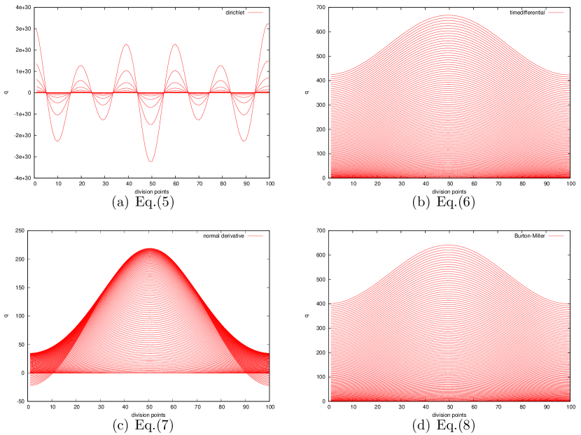
Figure 1: $q$ obtained with various integral equations vs point number. The point number and the azimuth angle $\theta$ are related by $\theta=-2\pi/100\times{}$ point number

Figure 2: “Exact” solution of $q$

We next check the behaviour of the characteristic roots of these time domain BIEs using SSM. We set the range for computing eigenvalues to be $0\leq\mathrm{Re}\ \Omega\leq 50=\frac{\pi}{\Delta t}$ and $-2\leq\mathrm{Im}\ \Omega\leq 2$ considering the periodicity of (13) and the fact that the characteristic roots are located symmetrically with respect to the imaginary axis, which can be easily shown using the explicit forms of (13). Note that the upper limit of $\Omega$ is consistent with the Nyquist frequency associated with $\Delta t$. Also, we took $n_{\mathrm{max}}$ to be 60 considering the number of boundary subdivisions and the spatial Nyquist “frequency”. In the computation, we redefine the Hankel functions so that they have branch cuts on the negative imaginary axis rather than on the negative real axis. This guarantees that the expression in (13) is analytical when $0<\mathrm{Re}\,\Omega<\frac{\pi}{\Delta t}$ holds.

Figs.3(a)–Fig.3(d) show the characteristic roots of the BIEs in (5)–(8), respectively. We plot the eigenvalues of (13) for various BIEs (i.e., zeros of the expressions in (17)–(20)) in green and the eigenvalues of the frequency domain BIEs given by $\hat{K}(\Omega)v=0$ (i.e., zeros of the products of Hankel and Bessel functions obtained by setting $m=0$ in (17)–(20)) in red.

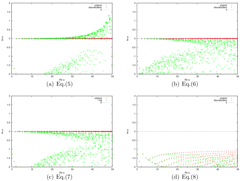
Figure 3: Characteristic roots of various integral equations

Note that the red symbols near the imaginary axis in Figs.3(a)–Fig.3(d) are the true eigenvalues for the exterior Dirichlet problem, while those on the real axis are fictitious ones related to the interior Dirichlet problems in Figs.3(a) and 3(b) and to the Neumann problem in Fig.3(c). The fictitious eigenvalues for (8) are those associated with interior impedance boundary value problems. We note that all BIEs in (5)–(8) have characteristic roots close to the true or fictitious eigenvalues, but other characteristic roots are scattered and quite far from any of eigenvalues of the corresponding frequency domain BIEs, except in the BM equation in (8).

From these figures, we see that the BIE (5) has the characteristic roots with positive imaginary parts, but this is not the case with other BIEs. These results are consistent with the corresponding time domain results. Also, the inaccuracy of (7) is considered to be related to the fact that $\Omega=0$ is an eigenvalue of (19) with $n=0$. We remark that a similar case has been reported in Parot et al.[6] where this phenomenon has been called a “pneumatic mode”. As a matter of fact $\Omega=0$ is a zero of both (18) (for all $n$) and (20) (for $n=0$) as well. An adverse effect of this eigenvalue on (8) is visible in the constant shift of the solution in Fig.1(d), although not as evidently as in Fig.1(c).

To examine the effect of this zero eigenvalue on the numerical solution of (6), we consider another incident wave given by

$$u^{\mathrm{inc}}=\begin{cases}0&(c_{1}t-x_{1}-t_{0}\leq 0)\\ \frac{(c_{1}t-x_{1}-t_{0})^{2}}{c_{1}t-x_{1}-t_{0}+4\Delta t}&(c_{1}t-x_{1}-t_{0}>0),\end{cases}$$ (22)

which is a smoothed linear function, where $t_{0}=1+2\Delta t$. Setting other parameters the same as in the previous example, we solve (6) to compute the time history of $q$ as plotted in Fig.4(a). Comparing this result with the “exact” solution given in Fig.4(c) one sees that an error having a zig-zag pattern is superimposed on the solution of (6). This is in contrast to the BM solution given in Fig.4(b) which is smooth. This result can be explained as follows. With (6), the (spatially) high frequency error incurred initially by the mismatch of the wavefront and mesh remains undamped after a long time because of the existence of a zero characteristic root with high $n$ eigenfunctions. Since this eigenvalue is zero, this error does not propagate, decay or amplify. In other words, it persists. This type of error is included also in Fig.1(b), although its magnitude is too small to be visible. From these numerical experiments, we conclude that none of the integral equations in (5)–(8) are satisfactory!

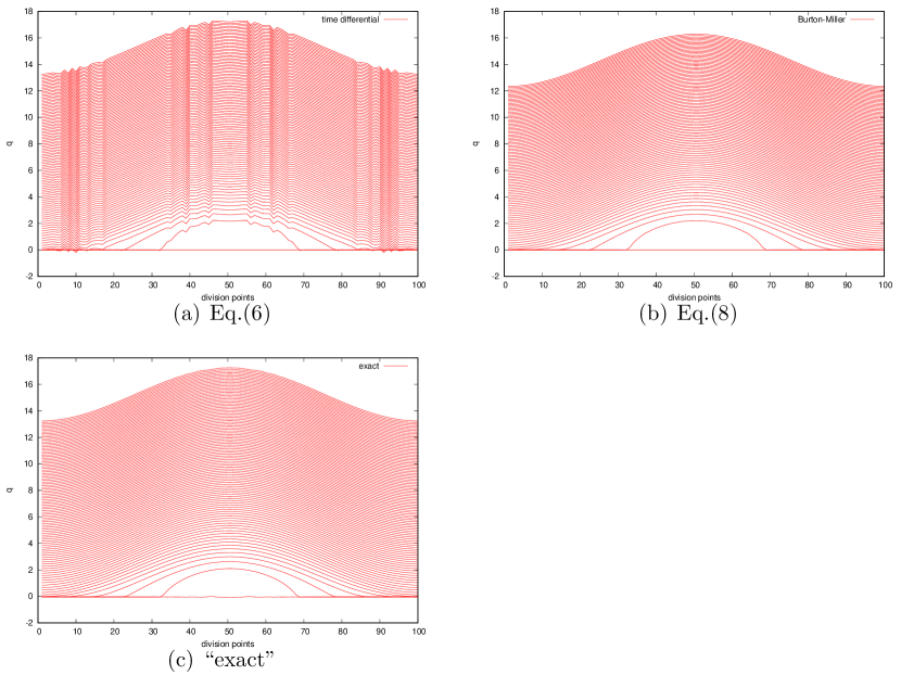
Figure 4: $q$ obtained with various integral equations

A possible remedy for all these problems is to use an integral equation given by

$$\frac{\partial u^{\mathrm{inc}}}{\partial n}(x,t) +\frac{1}{c_{1}}\dot{u}^{\mathrm{inc}}(x,t)+\alpha{u}^{\mathrm{inc}}(x,t)$$

$$-(D^{T1})^{-}q(x,t)-\frac{1}{c_{1}}\dot{S}^{1}q(x,t)-\alpha S^{1}q(x,t)=0,$$ (23)

which is the time domain counterpart of the BM equation with a complex (not pure imaginary) coupling constant, where $\alpha$ is a (real) number. It is easy to see that $\Omega=0$ is not a characteristic root of this equation. The numerical solution $q$ obtained with (2.5) and the incident wave in (22) is given in Fig.5(a) and its characteristic roots are shown in Fig.5(b), where we set $\alpha=1$.

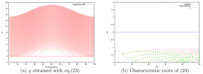
Figure 5: Augmented BM integral equation

The high accuracy and stability of this formulation is evident from these figures.

Epstein et al.[29] investigated time domain integral equations whose solutions exhibit correct long-time behaviours. From this viewpoint, (2.5) seems to be a better choice than other stable choices in (6)–(8), although the characteristic root of (2.5) whose imaginary part has the minimum magnitude is close to one of fictitious eigenvalues (the one whose imaginary part is approximately equal to -0.8) rather than a true one.

3 “Stable potentials”

Motivated by the results in the previous section, we examine the stability of integral equations on the unit circle derived from potentials which may appear in BIEs. These potentials include the single layer $S\,(=S^{+}=S^{-})$, traces of the normal derivatives of $S$ denoted by $D^{T\pm}$, the time derivative of $S$ denoted by $\dot{S}\,(=\dot{S}^{+}=\dot{S}^{-})$ and the traces of the double layer $D^{\pm}$. Although we are also interested in the normal derivative of $D$ denoted by $N$, it turned out that the simplified approach presented in 2.4 using the Fourier series expansion is not very easy to apply to $N$ with piecewise linear time basis functions because the series similar to (17)–(19) for $N$ does not converge absolutely (A similar observation applies to $\dot{D}^{\pm}$ as well). Using a smoother time basis function could be a solution. As we shall see later, however, the time integrated normal derivative of the double layer potential defined by

$$Mu=\int_{0}^{t}\int_{\Gamma}\frac{\partial}{\partial n_{x}}\frac{\partial}{\partial n_{y}}\log\frac{c(t-s)+\sqrt{c^{2}(t-s)^{2}-|x-y|^{2}}_{+}}{|x-y|}u(y,s)dS_{y}ds$$

$$x\in\mathbb{R}^{2}\setminus\Gamma,\quad t>0$$

is more useful than $N$ as far as the stability is concerned. We therefore carry out the stability analysis in 2.4 with $M\,(=M^{+}=M^{-})$ instead of $N$. Since the results for $S$, $\dot{S}$ and $D^{T-}=D^{+}$ have already been given in Figs.3(a)–3(c), we present those for $D^{T+}=D^{-}$ and $M$ in Figs.6(a)–6(b) using the same time increment as before (i.e., $\Delta t=2\pi/100$). They are zeros of the following expressions.

$$D^{-},\,D^{T+}\leftrightarrow f_{3}(\Omega;n,c)=\sum_{m}\Omega_{m}/cH_{n}^{(1)^{\prime}}(\Omega_{m}/c)J_{n}(\Omega_{m}/c)\hat{\phi}_{\Delta t}(\Omega_{m})$$ (24)

$$M\leftrightarrow f_{4}(\Omega;n,c)=\sum_{m}i\Omega_{m}/c^{2}H_{n}^{(1)^{\prime}}(\Omega_{m}/c)J^{\prime}_{n}(\Omega_{m}/c)\hat{\phi}_{\Delta t}(\Omega_{m})$$ (25)

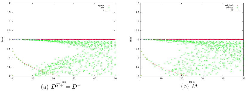
Figure 6: Characteristic roots of various integral operators

From these results, we confirm that the equations obtained by discretising the following integral equations are numerically stable with piecewise linear time basis functions: (a) the time derivative of the single layer potential (b) the interior and exterior traces of the normal derivative of the single layer potential (c) the interior and exterior traces of the double layer potential (d) the time integrated normal derivative of the double layer potential. Note, however, that we have no claim of stability of these potentials except in the cases tested here.

In the next section, we combine these “stable potentials” to obtain numerically stable formulations in transmission problems.

4 Transmission problems

We are now interested in finding $u$ which satisfies (1),

$$\Delta u-\frac{1}{c_{2}^{2}}\frac{\partial^{2}u}{{\partial t}^{2}}=0\hskip 5.69046pt\mathrm{in}\ D_{2}\times(t>0),$$

the transmission boundary conditions on $\Gamma$:

$$u^{+}=u^{-}(=u),\quad s_{1}\frac{\partial u^{+}}{\partial n}=s_{2}\frac{\partial u^{-}}{\partial n}\ (=q)\quad\mbox{ on }\Gamma\times(t>0)$$

and the homogeneous initial conditions

$$u|_{t=0}=\dot{u}|_{t=0}=0\qquad\mbox{in }D_{2}$$

in addition to the homogeneous initial and radiation conditions for $u^{\mathrm{sca}}$ in (2), where $c_{2}$ is the wave speed in $D_{2}$ given by $c_{2}=\sqrt{\frac{s_{2}}{\rho_{2}}}$ and ($s_{2}$, $\rho_{2}$) are the shear modulus and density in $D_{2}$, respectively. The superscript $+(-)$ stands for the trace to $\Gamma$ from $D_{1}$ ($D_{2}$), respectively.

4.1 Boundary integral equations

There exist various possibilities of integral equation for transmission problems on $\Gamma$, of which we consider the following four [25, 26]:

PMCHWT

$$\left(\begin{array}[]{cc}-(D^{1}+D^{2})&\frac{1}{s_{1}}S^{1}+\frac{1}{s_{2}}S^{2}\\ -(s_{1}N^{1}+s_{2}N^{2})&D^{T1}+D^{T2}\end{array}\right)\left(\begin{array}[]{c}u\\ q\end{array}\right)=\left(\begin{array}[]{c}u^{\mathrm{inc}}\\ s_{1}\frac{\partial u^{\mathrm{inc}}}{\partial n}\end{array}\right)$$ (32)

Müller

$$\left(\begin{array}[]{cc}\frac{s_{1}+s_{2}}{2}-(s_{1}D^{1}-s_{2}D^{2})&S^{1}-S^{2}\\ -(N^{1}-N^{2})&\frac{s_{1}+s_{2}}{2s_{1}s_{2}}+\frac{1}{s_{1}}D^{T1}-\frac{1}{s_{2}}D^{T2}\end{array}\right)\left(\begin{array}[]{c}u\\ q\end{array}\right)=\left(\begin{array}[]{c}s_{1}u^{\mathrm{inc}}\\ \frac{\partial u^{\mathrm{inc}}}{\partial n}\end{array}\right)$$ (39)

Burton-Miller

$$\left(\begin{array}[]{cc}\frac{1}{2c_{1}}\frac{\partial}{\partial t}-(N^{1}+\frac{1}{c_{1}}\dot{D^{1}})&\frac{1}{2s_{1}}+\frac{1}{s_{1}}D^{T1}+\frac{1}{c_{1}s_{1}}\dot{S^{1}}\\ -\frac{1}{2}-D^{2}&\frac{1}{s_{2}}S^{2}\end{array}\right)\left(\begin{array}[]{c}u\\ q\end{array}\right)=\left(\begin{array}[]{c}\frac{\partial u^{\mathrm{inc}}}{\partial n}+\frac{1}{c_{1}}\frac{\partial u^{\mathrm{inc}}}{\partial t}\\ 0\end{array}\right)$$ (46)

standard

$$\left(\begin{array}[]{cc}\frac{1}{2}-D^{1}&\frac{1}{s_{1}}S^{1}\\ \frac{1}{2}+D^{2}&-\frac{1}{s_{2}}S^{2}\end{array}\right)\left(\begin{array}[]{c}u\\ q\end{array}\right)=\left(\begin{array}[]{c}u^{\mathrm{inc}}\\ 0\end{array}\right)$$ (53)

In these equations we write $D^{\nu}$ for $(D^{\nu+}+D^{\nu-})/2$ etc. in order to show the non-integral terms explicitly at the cost of an abuse of notation. We note that there exist several versions of Müller’s formulations for the wave equation. We here use the one in which the singularities of single layer potentials cancel.

4.2 Stable formulations

The boundary integral equations shown in the previous section can be rewritten easily in terms of “stable potentials” presented in section 3 with the help of time differentiation and integration by parts. Here are the results:

modified PMCHWT

$$\left(\begin{array}[]{cc}-(D^{1}+D^{2})&\frac{1}{s_{1}}\dot{S}^{1}+\frac{1}{s_{2}}\dot{S}^{2}\\ -(s_{1}M^{1}+s_{2}M^{2})&D^{T1}+D^{T2}\end{array}\right)\left(\begin{array}[]{c}\dot{u}\\ q\end{array}\right)=\left(\begin{array}[]{c}\dot{u}^{\mathrm{inc}}\\ s_{1}\frac{\partial u^{\mathrm{inc}}}{\partial n}\end{array}\right)$$ (60)

modified Müller

$$\left(\begin{array}[]{cc}\frac{s_{1}+s_{2}}{2}-(s_{1}D^{1}-s_{2}D^{2})&\dot{S}^{1}-\dot{S}^{2}\\ -(M^{1}-M^{2})&\frac{s_{1}+s_{2}}{2s_{1}s_{2}}+\frac{1}{s_{1}}D^{T1}-\frac{1}{s_{2}}D^{T2}\end{array}\right)\left(\begin{array}[]{c}\dot{u}\\ q\end{array}\right)=\left(\begin{array}[]{c}s_{1}\dot{u}^{\mathrm{inc}}\\ \frac{\partial u^{\mathrm{inc}}}{\partial n}\end{array}\right)$$ (67)

modified Burton-Miller

$$\left(\begin{array}[]{cc}\frac{1}{2c_{1}}-(M^{1}+\frac{1}{c_{1}}{D^{1}})&\frac{1}{2s_{1}}+\frac{1}{s_{1}}D^{T1}+\frac{1}{c_{1}s_{1}}\dot{S^{1}}\\ -\frac{1}{2}-D^{2}&\frac{1}{s_{2}}\dot{S}^{2}\end{array}\right)\left(\begin{array}[]{c}\dot{u}\\ q\end{array}\right)=\left(\begin{array}[]{c}\frac{\partial u^{\mathrm{inc}}}{\partial n}+\frac{1}{c_{1}}\frac{\partial u^{\mathrm{inc}}}{\partial t}\\ 0\end{array}\right)$$ (74)

modified standard

$$\left(\begin{array}[]{cc}\frac{1}{2}-D^{1}&\frac{1}{s_{1}}\dot{S}^{1}\\ \frac{1}{2}+D^{2}&-\frac{1}{s_{2}}\dot{S}^{2}\end{array}\right)\left(\begin{array}[]{c}\dot{u}\\ q\end{array}\right)=\left(\begin{array}[]{c}\dot{u}^{\mathrm{inc}}\\ 0\end{array}\right)$$ (81)

where $M^{\nu}$ is the time integral of $N^{\nu}$.

The PMCHWT, Müller and BM formulations are known not to have real fictitious eigenfrequencies in the frequency domain, while the standard formulation does have real fictitious eigenfrequencies[25, 26]. It is therefore expected that the standard formulation is more prone to instability.

We remark that the time differentiated standard integral equation in the modified standard equation (81) has appeared in the paper by Panagiotopoulos and Manolis[13] on elastodynamics in 3D. Also, the combined use of of $D$, $\dot{S}$, $M$ and $D^{T}$ in (60), (67) and (74) has been proposed by Abboud et al.[3] and Banjai et al.[20] in different contexts in 3D. Their choices of unknowns are different from ours. To the best of our knowledge, however, these potentials have not been utilised in forms given in (60), (67) and (74) in transmission problems for the wave equation in 2D.

4.3 Numerical experiments

Setting $s_{1}=1$, $\rho_{1}=1$, $s_{2}=0.2$ and $\rho_{2}=0.37$, we solve the time domain BIEs in (32)–(81). The incident wave is the quadratic one in (21) and the number of boundary subdivisions, the number of time steps and the time increments are the same as in 2.5. We use piecewise linear time basis functions for ($u,q$) in the ordinary formulations and for ($\dot{u},q$) in the modified formulations.

Fig.7 and Fig.8 show the results of $q$ obtained with the ordinary and modified integral equations respectively. We see that the ordinary formulations give unstable results except for the Müller formulation, whereas all the modified formulations provide stable results.

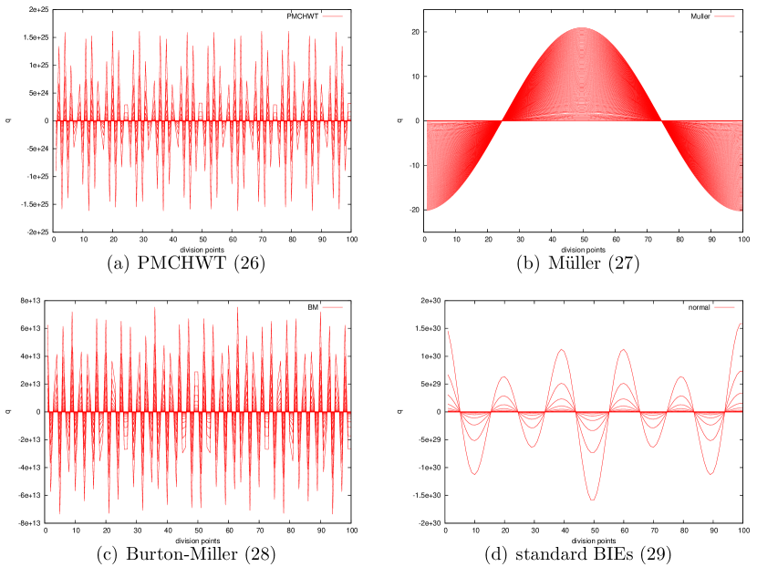
Figure 7: $q$ obtained with ordinary integral equations for transmission problems

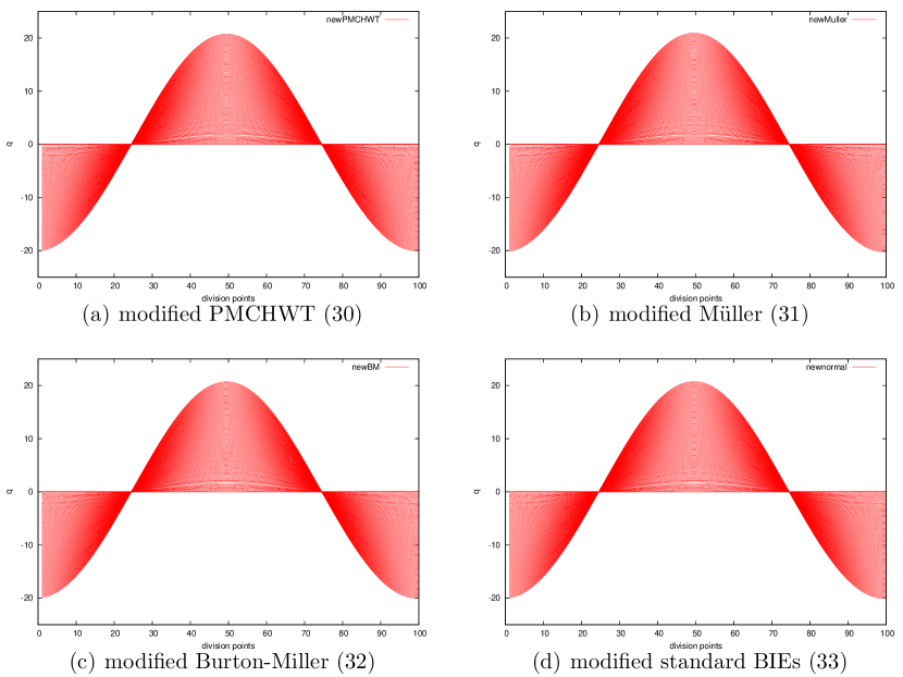
Figure 8: $q$ obtained with modified integral equations for transmission problems

Fig.9 shows the distribution of characteristic roots for those formulations which do not include $N$ or $\dot{D}$. In the modified PMCHWT, for example, they are obtained as the non linear eigenvalues ($\Omega$’s) of the following matrix for one of $n=0,\cdots,n_{\mathrm{max}}$. See (18), (19), (24) and (25):

$$\tilde{K} (\Omega;n)_{\mathrm{PMCHWT}}=$$

$$\left(\begin{array}[]{cc}-(f_{3}(\Omega;n,c_{1})+f_{2}(\Omega;n,c_{2}))&\frac{1}{s_{1}}f_{1}(\Omega;n,c_{1})+\frac{1}{s_{2}}f_{1}(\Omega;n,c_{2})\\ -(s_{1}f_{4}(\Omega;n,c_{1})+s_{2}f_{4}(\Omega;n,c_{2}))&f_{2}(\Omega;n,c_{1})+f_{3}(\Omega;n,c_{2})\end{array}\right)$$ (84)

The distribution of characteristic roots shown in Fig.9 is seen to be consistent with the time domain results in Figs.7 and 8. These results also suggest that the use of standard BIEs may not be recommended even after the modification since this formulation has many characteristic roots near the real axis.

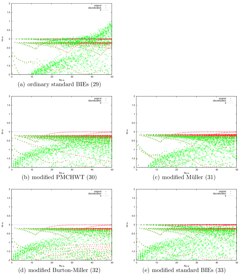
Figure 9: Characteristic roots of various integral equations for transmission problems

Among other three formulations the Müller formulation appears to be better in terms of stability since it gives stable results even without modification, as one sees in Figs.7 and 8. Another reason to prefer Müller is the behaviour of the characteristic equations (4.3), etc., near $\Omega=0$. As a matter of fact, we can show that $\Omega=0$ is a characteristic root of BM for $n=0$, but other two do not suffer from this problem. However, the characteristic equation (4.3) for the modified PMCHWT has the following asymptotic behaviour near $\Omega=0$:

$$\tilde{K}(\Omega;n)_{\mathrm{PMCHWT}}=\left(\begin{array}[]{cc}o(\Omega)&O(\Omega)\\ O(1/\Omega)&o(\Omega)\end{array}\right)\qquad n\geq 1$$ (87)

while $\tilde{K}(\Omega;0)_{\mathrm{PMCHWT}}=O(1)$. This means that the vector $(0,1)^{T}$ behaves asymptotically like an eigenvector of (87) for $\Omega\approx 0$. This suggests that an arbitrary error of $q$ having a zero spatial mean may persist in the solution of the modified PMCHWT. For the modified Müller equation, however, there is no problem of this kind since we have

$$\tilde{K}(\Omega;n)_{\text{M\"{u}ller}}=\left(\begin{array}[]{cc}O(1)&o(1)\\ o(1)&O(1)\end{array}\right).$$

We thus conclude that the modified Müller equation is a better choice than the other two in the cases tested.

To confirm this conclusion, we use the modified PMCHWT and Müller equations to solve the same transmission problem as in Figs.7 and 8 after replacing the incident wave by the quasi-linear one in (22). As has been expected, the modified PMCHWT result includes persistent noise, while the modified Müller result is smooth as shown in Fig.10. Further details of this subject will be presented elsewhere.

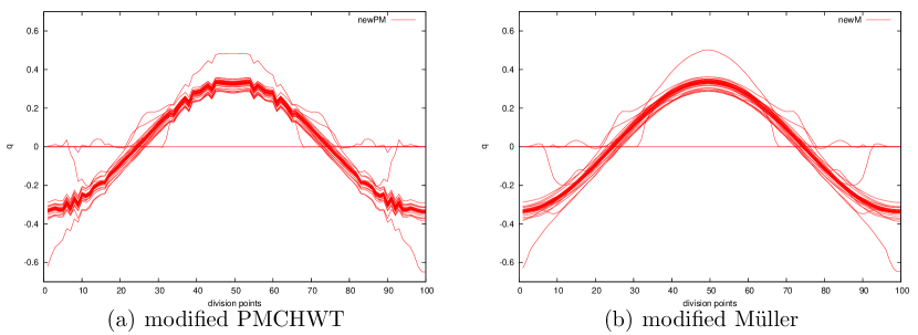
Figure 10: $q$ obtained with modified PMCHWT and Müller formulations

5 Effects of space discretisation

So far, we have neglected the effect of spatial discretisation in the discussion of stability. This section discusses how the distribution of the eigenvalues is influenced by the space discretisation. We restrict our attention to the circular scatterer case using the Fourier series expansion in order to keep the discussion as analytical as possible so that we can obtain insights.

5.1 Formulation

We consider a circular boundary having a radius of $1$ with $N$ piecewise constant arc elements whose endpoints (angles) are given as $\theta=\theta_{1},\cdots,\theta_{N}$ ($\theta_{N+1}=\theta_{1}$). We consider an integral operator $K(\Omega)$ which maps a function $v$ on the boundary to another function on the boundary. The function $v$ is then approximated with the piecewise constant basis function on each element as follows:

$$v(\theta)\approx\sum_{p=1}^{N}v_{p}N_{p}(\theta),\ N_{p}(\theta)=\left\{\begin{array}[]{cc}1&\theta\in[\theta_{p},\theta_{p+1}]\\ 0&\mbox{otherwise}\end{array}\right.$$

where $\theta$ is the angular coordinate of the position on the boundary. This is considered to be a reasonable approximation of the discretisation with straight line boundary elements. The basis function is now expanded into the Fourier series given by:

$$N_{p}(\theta)\approx\sum_{l=-M}^{M}V_{l}^{p}e^{il\psi}$$

where $M$ is the truncation number of the infinite Fourier series and $V_{l}^{p}$ is the coefficient of the Fourier series given as follows:

$$V_{l}^{p}=\frac{1}{2\pi}\int_{0}^{2\pi}e^{-il\psi}N_{p}\,d\psi=\frac{1}{2\pi}\int_{\theta_{p}}^{\theta_{p+1}}e^{-il\psi}\,d\psi.$$

Suppose that $K$ is an integral operator for layer potentials such as $\hat{S}$, $\hat{M}$, etc., in frequency domain. Then the value of $Kv$ at a collocation point $\Theta_{n}=(\theta_{n}+\theta_{n+1})/2$ is given as

$${K}v|_{\Theta_{n},n=1,\cdots,N}=\sum_{p=1}^{N}\sum_{l=-M}^{M}e^{il\Theta_{n}}\{HJ\}_{l}V_{l}^{p}v_{p}.$$ (88)

where $\{HJ\}_{l}$ stands for the product of Hankel and Bessel functions (or their derivatives) with appropriate coefficients. The $\{HJ\}$’s for the integral operators used in this paper are given as follows:

$$S^{\nu}\leftrightarrow H_{n}^{(1)}(k_{\nu})J_{n}(k_{\nu})$$

$$\dot{S}^{\nu}\leftrightarrow-i\Omega H_{n}^{(1)}(k_{\nu})J_{n}(k_{\nu})$$

$$D^{\nu-},\,D^{T\nu+}\leftrightarrow k_{\nu}H_{n}^{(1)^{\prime}}(k_{\nu})J_{n}(k_{\nu})$$

$$D^{\nu+},\,D^{T\nu-}\leftrightarrow k_{\nu}H_{n}^{(1)}(k_{\nu})J^{\prime}_{n}(k_{\nu})$$

$$M^{\nu}\leftrightarrow-k^{2}_{\nu}H_{n}^{(1)^{\prime}}(k_{\nu})J^{\prime}_{n}(k_{\nu})/i/\Omega$$

The question of stability of the discretised integral operators in time domain is now reduced to the nonlinear eigenvalue problem for $\Omega$ for the following matrix:

$${\mathsf{U}}\left(\begin{array}[]{ccc}\mathcal{D}_{-M}&&0\\ &\ddots&\\ 0&&\mathcal{D}_{M}\end{array}\right){\mathsf{V}}$$ (92)

where $\mathsf{V}$ ($\mathsf{U}$) is a $(2M+1)\times N$ ($N\times(2M+1)$) matrix whose $(l,p)$ ($(n,l)$) components are given by

$${\mathsf{V}}_{lp}=V_{l}^{p}\quad({\mathsf{U}}_{nl}=e^{il\Theta_{n}})$$

and

$$\mathcal{D}_{l}=\sum_{m=-\infty}^{\infty}\{HJ\}_{l}\left(\Omega-\frac{2m\pi}{\Delta t}\right)\hat{\phi}_{\Delta t}\left(\Omega-\frac{2m\pi}{\Delta t}\right)$$

The corresponding matrices for the boundary integral equations for transmission problems can be obtained similarly. We can now solve the non-linear eigenvalue problem given by

$$K(\Omega)v=0$$

with the standard SSM.

5.2 Numerical experiments

We now show results of some numerical experiments. We consider various integral operators on the unit circle, setting $\rho=1,\ s=1$ and $\Delta t=2\pi/100$, respectively. The mesh on the boundary is uniform with $\theta_{p}=2\pi p/N,\ p=1,2,\cdots,N+1$. The number of boundary subdivision $N$ is set to be either $N=100$ or $N=200$. Accordingly, the truncation number of the Fourier series $M$ is set to be $M=10N+N/2$. Also, the infinite series $\sum_{m}\{HJ\}_{m}$ in (92) and similar ones for transmission problems are truncated with 100 terms since results obtained with 1000 terms were almost identical. We note that it is not very easy to calculate Bessel and Hankel functions of high order with large arguments included in this calculation. This problem is handled with the help of Exflib, a well-known multiple-precision library[30].

Figs. 11 show the eigenvalue distributions of various integral operators considered in section 3. The results with $N=100$ ($N=200$) are shown in triangular (circular) symbols and those without space discretisation (i.e., the characteristic roots given in previous sections, which we call “no space discretisation” in the rest of this paper) are given in cross symbols. It is seen that the property of eigenvalue distributions does not change very much regardless of the space discretisations. Namely, stable potentials seem to remain stable for reasonable spatial divisions. We also see that the $N=200$ results are closer to the no space discretisation results than those obtained with $N=100$. These observations justify the use of the no space discretisation method in the discussion of the stability of the time domain BIEMs.

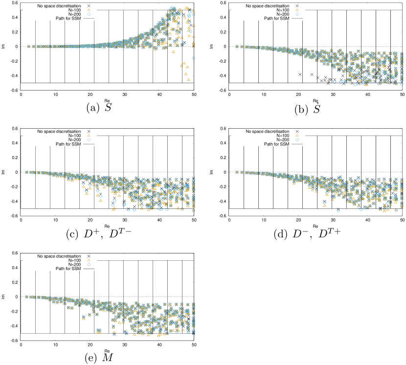
Figure 11: Eigenvalues of integral operators. $\times$: no space discretisation, $\triangle{}$: $N=100$, $\circ$: $N=200$

We next consider transmission problems. Figs. 12 show the eigenvalues of the modified boundary integral equations for transmission problems, i.e., modified PMCHWT (60), Müller (67), BM (74) and standard equations (81). We set $\rho_{1}=1,\ \rho_{2}=0.37,\ s_{1}=1,\ s_{2}=0.2$, and $\Delta t=2\pi/100$, respectively as in 4.3. Once again, the number of the spatial subdivision $N$ does not seem to change the distribution of the characteristic roots qualitatively. We therefore conclude that the stability of these formulations can be inferred from the no space discretisation results. Also, the finer the spatial discretisation the better approximation the no discretisation results become. We thus expect that further spatial discretisation is not likely to affect the stability of the modified boundary integral equations.

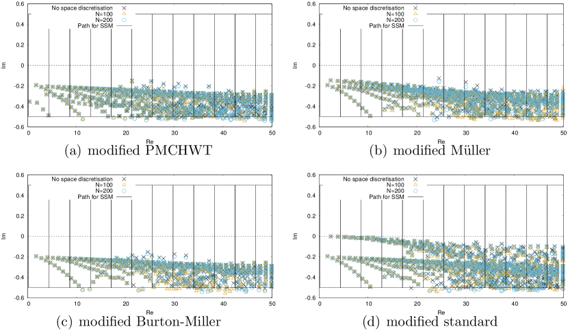
Figure 12: Eigenvalues of the modified integral equations for transmission problems. $\times$: no space discretisation, $\triangle{}$: $N=100$, $\circ$: $N=200$

6 Non circular boundary

Finally, we test if the modified formulations remain stable for boundaries other than circle. We consider transmission problems for a “star” (Fig.13(a)) given by

$$(x_{1},x_{2})=((1+0.3\cos{5\theta})\cos{\theta}/1.3,(1+0.3\cos{5\theta})\sin{\theta}/1.3)$$

and a “kite” (Fig.13(b)) given by

$$(x_{1},x_{2})=(0.18(\cos{\theta}+2(\cos{2\theta}-1)),0.72\sin{\theta}).$$

The incident wave is the quadratic one in (21) and parameters such as material constants, number of boundary subdivision, $\Delta t$ etc. are the same as those in the transmission problems considered in the last section. The boundary subdivision is uniform with respect to $\theta$.

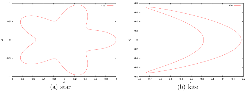
Figure 13: Domains

Fig.14 and Fig.15 show the distribution of $q$ on the boundary obtained with various formulations. Ordinary formulations except for Müller turn out to be unstable while modified formulations appear to be stable. Also, the results obtained with modified formulations basically agree with each other except for details. These comments apply as well to other cases which are not shown in the paper.

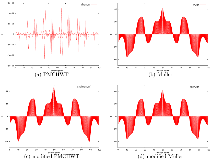
Figure 14: Transmission problems for “star”

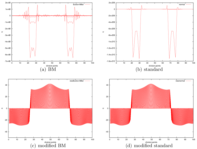
Figure 15: Transmission problems for “kite”

7 Concluding remarks

This paper revisited stability issues for BIEMs for the two dimensional wave equation in time domain. We presented a stability analysis based on integral equations in frequency domain and showed its validity and usefulness in simple exterior or transmission problems for circular domains. The resulting non-linear eigenvalue problems for the characteristic roots have been solved numerically with SSM. We identified layer potentials which lead to stable integral equations with linear time interpolation for our particular choices of parameters. Combining these potentials, we could formulate stable integral equations for transmission problems which include the velocity and the normal flux of the solution on the boundary as unknowns. Among integral equations considered the Müller formulation was concluded to be a better choice in cases tested. All these modified formulations were shown to remain stable in transmission problems for star and kite shaped boundaries.

We remark that we have no intention to claim that the combination of particular potentials always leads to stability or that the Müller formulation is always the best choice in transmission problems. What we showed in this paper is the fact that the proposed method of stability analysis in frequency domain is useful in investigating the stability and the accuracy of a time domain BIEM for the wave equation in 2D, given particular integral equations and discretisation methods. To be consistent with the purpose of this paper, we have restricted our attention to simple problems where we can utilise analytical tools as much as possible. Also, the numerical examples presented have been limited to small number of cases. Two obvious next steps, therefore, will be to consider more general boundaries and to carry out more extensive numerical experiments. The former investigation will include numerical treatment of (13) in which one considers integral equations having the function in (15) as the kernel instead of the fundamental solution in BIEs on general boundaries. Another interesting future direction is to test the modified formulations for transmission problems in 3D. As a matter of fact, we have already started investigations along this line. So far the same conclusions for stability as have been presented here seem to hold in 3D as well. Notice, however, that the use of the time domain stability analysis based on (12) may be simpler than the frequency domain approach in 3D (and, indeed, have already been utilised by many authors including Walker et al.[23], etc., as have been mentioned) because of the finite “tail” of the fundamental solution. We remark, however, that SSM will be useful in such stability analysis in time domain as well because one may apply it directly to a smaller eigenvalue problem in (11). We are also interested in the stability of interior problems in which true eigenvalues may cause instability[9], thus requiring different approaches than those utilised in this paper. Finally, we can mention investigations on the robustness of the algorithms as an important future research subject. As a matter of fact, we have carefully tried to eliminate errors in the present investigation. In real world applications, however, one has to use numerical integrations, truncated time steps, fast methods etc., which will inevitably introduce errors.

References

- [1] Bamberger A, Ha Duong T. Formulation variationnelle espace-temps pour le calcul par potentiel retardé de la diffraction d’un onde acoustique (I). Math Meth Appl Sci 1986;8:405–35.
- [2] Aimi A, Diligenti M, Guardasoni C. On the energetic Galerkin boundary element method applied to interior wave propagation problems. J Comp Appl Math 2011;235:1746–54.
- [3] Abboud T, Joly P, Rodríguez J, Terrasse I. Coupling discontinuous Galerkin methods and retarded potentials for transient wave propagation on unbounded domains, J Comp Phys 2011;230:5877–907.
- [4] van ’t Wout E, van der Huel DR, vander Ven H, Vuik C. Stability analysis of the marching-on-in time boundary element method for electromagnetics. J Comp Appl Math 2016;294:358–71.
- [5] Davies PJ, Duncan DB. Stability and convergence of collocation schemes for retarded potential integral equations. SIAM J Num Anal 2004;42:1167–88.
- [6] Parot JM, Thirard C, Puillet C. Elimination of a non-oscillatory instability in a retarded potential integral equation. Eng Anal Boundary Elements 2007;31:133–51.
- [7] Parot JM, Thirard C. A numerical algorithm to damp instabilities of a retarded potential integral equation. Eng Anal Boundary Elements 2011;35:691–9.
- [8] Jang H-W, Ih J-G. Stabilization of time domain acoustic boundary element method for the exterior problem avoiding the nonuniqueness. J Acoust Soc Am 2013;133:1237–44.
- [9] Jang H-W, Ih J-G. Stabilization of time domain acoustic boundary element method for the interior problem with impedance boundary conditions. J Acoust Soc Am 2012;131:2742–52.
- [10] Pak RYS, Bai X. A regularized boundary element formulation with weighted-collocation and higher-order projection for 3D time-domain elastodynamics. Eng Anal Boundary Elements 2018;93:135–42.
- [11] Bai X, Pak RYS. On the stability of direct time-domain boundary element methods for elastodynamics. Eng Anal Boundary Elements 2018;96:138–49.
- [12] Mansur WJ, Carrer JA, Siqueira EFN. Time discontinuous linear traction approximation in time-domain BEM scalar wave propagation analysis. Int J Num Meth Eng 1998;42:667–83.
- [13] Panagiotopoulos C, Manolis GD. Three-dimensional BEM for transient elastodynamics based on the velocity reciprocal theorem. Eng Anal Boundary Elements 2011;35:507–16.
- [14] Ergin AA, Shanker B, Michielssen E. Analysis of transient wave scattering from rigid bodies using a Burton-Miller approach. J Acoust Soc Am 1999;106:2396–404.
- [15] Chappell DJ, Harris PJ, Henwood H, Chakrabarti R. A stable boundary element method for modeling transient acoustic radiation. J Acoust Soc Am 2006;120:74–80.
- [16] Chappell DJ, Harris PJ. On the choice of coupling parameter in the time domain Burton-Miller formulation. Q J Mech Appl Math 2009;624:431–50.
- [17] Zhang Y, Bi C-X, Zhang Y-B, Zhang X-Z. Horn effect prediction on the time domain boundary element method. Eng Anal Boundary Elements 2017;82:79–84.
- [18] Lubich C. On the multistep time discretization of linear initial- boundary value problems and their boundary integral equations. Num Math 1994;67:365–89.
- [19] Sayas F-J. Retarded potentials and time domain boundary integral equations. Switzerland: Springer; 2010.
- [20] Banjai L, Lubich C, Sayas F-J. Stable numerical coupling of exterior and interior problems for the wave equation. Numer Math 2015;129:611–46.
- [21] Schanz M. Wave propagation in viscoelastic and poroelastic continua: a boundary element approach, Lecture Notes in Applied Mechanics. Berlin, Heidelberg, New York: Springer; 2001.
- [22] Wang H, Henwood DJ, Harris PJ, Chakrabarti R. Concerning the cause of instability in time-stepping boundary element methods applied to the exterior acoustic problem. J Sound Vibration 2007;305:289–97.
- [23] Walker SP, Bluck MJ, Chatzis I. The stability of integral equation time-domain computations for three-dimensional scattering; similarities and differences between electrodynamic and elastodynamic computations. Int J Num Modelling, Electronic Networks, Devices and Fields 2002;15:459–74.
- [24] Asakura J, Sakurai T, Tadano H, Ikegami T, and Kimura K. A numerical method for nonlinear eigenvalue problems using contour integrals. JSIAM Letters 2009;1:52–5.
- [25] Misawa R, Niino K, Nishimura N. An FMM for waveguide problems of 2-D Helmholtz’ equation and its application to eigenvalue problems. Wave Motion 2016;63:1-17.
- [26] Misawa R, Niino K, Nishimura N. Boundary integral equations for calculating complex eigenvalues of transmission problems. SIAM J Appl Math 2017;77:770–88.
- [27] Engquist B, Majda A. Absorbing boundary conditions for the numerical simulation of waves. Math Comp 1977;31:629–51.
- [28] Martin PA. Multiple scattering: interaction of time-harmonic waves with obstacles. Cambridge: Cambridge University Press; 2006.
- [29] Epstein CL, Greengard L Hagstrom T. On the stability of time-domain integral equations for acoustic wave propagation. Discrete Cont Dyn Sys-A 2016;36:4367–382.
- [30] http://www-an.acs.i.kyoto-u.ac.jp/ fujiwara/exflib/