2-parameter $\tau$-function for the first Painlevé equation
—Topological recursion and direct monodromy problem
via exact WKB analysis—

Abstract.

We show that a 2-parameter family of $\tau$-functions for the first Painlevé equation can be constructed by the discrete Fourier transform of the topological recursion partition function for a family of elliptic curves. We also perform an exact WKB theoretic computation of the Stokes multipliers of associated isomonodromy system assuming certain conjectures.

1. Introduction

Painlevé transcendents are remarkable special functions which appear in many areas of mathematics and physics. These are solutions of certain nonlinear ODEs known as Painlevé equations ([80]). Originally, there were six Painlevé equations (from Painlevé I to Painelvé VI), but now several generalizations of the Painlevé equations (($q$-)discrete, elliptic, higher order analogues) are discovered (see [32, 41, 64, 77, 82, 83] for instance). More than 100 years have passed since the discovery of the Painlevé equations, and lots of beautiful properties have been revealed through various approaches (isomonodromic deformation, Riemann-Hilbert method, affine-Weyl symmetry, the space of initial conditions, and so on). However, even for the classical six Painlevé equations, there are still several open problems to be considered (see [19] for example).

A surprising development has been achieved in 2012 by Gamayun-Iorgov-Lisovyy ([34]). They studied the Painlevé VI equation

$$\frac{d^{2}q}{dt^{2}} =\frac{1}{2}\biggl{(}\frac{1}{q}+\frac{1}{q-1}+\frac{1}{q-t}\biggr{)}\cdot\biggl{(}\frac{dq}{dt}\biggr{)}^{2}-\biggl{(}\frac{1}{t}+\frac{1}{t-1}+\frac{1}{q-t}\biggr{)}\cdot\frac{dq}{dt}$$

$$\quad+\frac{2q(q-1)(q-t)}{t^{2}(t-1)^{2}}\cdot\left(\Bigl{(}\theta_{\infty}-\frac{1}{2}\Bigr{)}^{2}-\frac{\theta_{0}^{2}\,t}{q^{2}}+\frac{\theta_{1}^{2}\,(t-1)}{(q-1)^{2}}-\frac{\bigl{(}\theta_{t}^{2}-\frac{1}{4}\bigr{)}\,t(t-1)}{(q-t)^{2}}\right),$$ (1.1)

and obtained the following formula for the $\tau$-function ([56, 78]) corresponding to 2-parameter general solutions of Painlevé VI:

$$\tau_{P_{\rm VI}}(t,\vec{\theta},\nu,\rho)=\sum_{k\in{\mathbb{Z}}}e^{2\pi ik\rho}\cdot B(t,\vec{\theta},\nu+k).$$ (1.2)

Here $B$ is a 4-point Virasoro conformal block with $c=1$ which has an explicit combinatorial formula (see [34, (1.8)–(1.12)]); this is a consequence of the Alday-Gaiotto-Tachikawa correspondence [1] and the Nekrasov’s formula [75]. The constants $\vec{\theta}=(\theta_{0},\theta_{1},\theta_{t},\theta_{\infty})$ are related to characteristic exponents of the associated isomonodromy system. The two parameters $\nu$ and $\rho$ are the integration constants which specify initial conditions in solving Painlevé VI. It is very interesting that the general solution can be expressed as a discrete Fourier transform, and it is highly non-trivial from a glance of (1.1).

After the work [34], the Painlevé equations attract much more researchers in the community of the conformal field theory, gauge theory, topological string theory, and so on. Similar formulas to (1.2) are also obtained or conjectured, for other Painlevé equations. For instance, Gamayun-Iorgov-Lisovyy also find a similar explicit formula for Painlevé V and III in [35]. Nagoya gave a conjectural expression of Painlevé II–V as a discrete Fourier transform of irregular conformal blocks in [71, 72] (see also [67]). Bonelli-Lisovyy-Maruyoshi-Sciarappa-Tanzini ([9]) also gave conjectural expressions for Painlevé I, II, and IV as a discrete Fourier transform of a partition function of Argyres-Douglas theories. Regarding on higher order and $q$-analogues, we refer [7, 8, 36, 37, 57, 70].

On the other hand, Eynard-Orantin’s topological recursion ([29]) is a recursive algorithm to compute the 1/N-expansion of the correlation functions and the partition function of matrix models from its spectral curve (c.f., [17]), and it is generalized to any algebraic curve which may not come from a matrix model. The topological recursion attracts both mathematicians and physicists since it is expected to encode the information of various enumerative and quantum invariants (e.g., Gromov-Witten invariants, Hurwitz numbers, Jones polynomials, and so on) in a universal way. It is also related to integrable systems ([10]), the WKB analysis through the theory of quantum curves ([12, 26, 76] etc.), and several topics in mathematics and physics. See the review article [30] for further information.

Relationships between the topological recursion and Painlevé equations has been discussed in [29, 54] for Painlevé I, [50] for Painlevé II, and [51] for Painlevé I–VI. In these articles, the Painlevé $\tau$-functions are constructed as the partition function of the topological recursion applied to spectral curves arising in the WKB analysis of associated isomonodromy systems. These results are generalized to a class of Painlevé hierarchies with rank 2 isomonodromy systems by [69] recently.

However, the Painlevé $\tau$-functions constructed by topological recursion are particular solutions. More precisely, such solutions admit a power series expansion (without any exponential terms). Then, it is easy to see that the expansion coefficients are recursively determined; that is, such solutions cannot contain any of integration constants (thus they are called “0-parameter solutions”). This reflects the fact that the all spectral curves considered in those works are of genus $0$. Hence, it is natural to ask:

Can we generalize the relationship between the Painlevé equations and the topological recursion in such a way that we can handle the 2-parameter solutions like (1.2) ?

A candidate of such a framework is proposed by Borot-Eyanrd [10] in a relationship between the topological recursion and integrable systems, where the discrete Fourier transform of the partition function is introduced. The discrete Fourier transform has also considered in an equivalent but different expression by Eynard-Marinõ [28], which is called the non-perturbative partition function. However, in these works, a precise relationship to Painlevé equations has not been discussed.

The purpose of this paper is, based on the ideas by [10, 28], to answer the above question affirmatively for the Painlevé I equation

$$(P_{\rm I})~{}:~{}\hbar^{2}\frac{d^{2}q}{dt^{2}}=6q^{2}+t$$ (1.3)

with a formal parameter $\hbar$ being appropriately introduced. That is, we will construct a 2-parameter family of (formal) $\tau$-functions for Painlevé I by using the framework of the topological recursion and the quantum curves applied for a genus $1$ spectral curve. We will also see that a Fourier series structure, which was conjectured in [9], appears in the expression of the $\tau$-function, and in the WKB analysis of isomonodromy systems.

The precise statements of our main results are formulated as follows. Let us consider a family of smooth elliptic curves (with a fixed generator $A,B$ of their first homology group)

$$y^{2}=4x^{3}+2tx+u(t,\nu),$$ (1.4)

with $u(t,\nu)$ being chosen so that the $A$-period

$$\nu:=\frac{1}{2\pi i}\oint_{A}ydx$$ (1.5)

is independent of $t$. It is regarded as the spectral curve for the topological recursion via the standard Weierstrass parametrization:

$$\begin{cases}x=\wp(z;g_{2},g_{3})\\ y=\wp^{\prime}(z;g_{2},g_{3})\end{cases}\quad\text{with}\quad g_{2}=-2t,\quad g_{3}=-u(t,\nu).$$ (1.6)

Let $W_{g,n}(z_{1},\dots,z_{n})$ and $F_{g}$ be the correlator of type $(g,n)$ and the $g$-th free energy defined by the Eyanrd-Orantin topological recursion applied to the spectral curve, respectively (see §3.2 for the definition). Let us also define two formal series of $\hbar$ by

$$Z(t,\nu;\hbar):=\exp\Biggl{(}\sum_{g\geq 0}\hbar^{2g-2}F_{g}(t,\nu)\Biggr{)}$$ (1.7)

and

$$\psi(x,t,\nu;\hbar):=\exp\Biggl{(}\,\frac{1}{\hbar}\int^{z(x)}_{0}W_{0,1}(z)+\frac{1}{2}\int^{z(x)}_{0}\int^{z(x)}_{0}\left(W_{0,2}(z_{1},z_{2})-\frac{dx(z_{1})\cdot dx(z_{2})}{(x(z_{1})-x(z_{2}))^{2}}\right)\\ +\sum_{\begin{subarray}{c}g\geq 0,\,n\geq 1\\ 2g-2+n\geq 1\end{subarray}}\frac{\hbar^{2g-2+n}}{n!}\int^{z(x)}_{0}\cdots\int^{z(x)}_{0}W_{g,n}(z_{1},\cdots,z_{n})\Biggr{)}.$$ (1.8)

Here $z(x)$ is the inverse function of $x=\wp(z)$. The formal series $Z$ is called the topological recursion partition function. The other formal series $\psi$ (which is called the wave function in literature of quantum curves) is a WKB-type formal solution of a linear PDE (Theorem 3.7).

Then our main results are formulated as follows:

Main Theorem (Theorem 4.3 and Theorem 4.5).

• The formal series

  $$\tau_{P_{\rm I}}(t,\nu,\rho;\hbar):=\sum_{k\in{\mathbb{Z}}}e^{{2\pi ik\rho}/{\hbar}}\cdot Z(t,\nu+k\hbar;\hbar)$$ (1.9)

  is a formal $\tau$-function of $(P_{\rm I})$. In other words, the formal series

  $$q(t,\nu,\rho;\hbar):=-\hbar^{2}\frac{\partial^{2}}{\partial t^{2}}\log\tau_{P_{\rm I}}(t,\nu,\rho;\hbar)$$ (1.10)

  satisfies $(P_{\rm I})$.

• The formal series

  $$\Psi(x,t,\nu,\rho;\hbar):=\frac{\sum_{k\in{\mathbb{Z}}}e^{{2\pi ik\rho}/{\hbar}}\cdot Z(t,\nu+k\hbar;\hbar)\cdot\psi(x,t,\nu+k\hbar;\hbar)}{\sum_{k\in{\mathbb{Z}}}e^{{2\pi ik\rho}/{\hbar}}\cdot Z(t,\nu+k\hbar;\hbar)}$$ (1.11)

  is a formal solution of the isomonodrmy system

  $$(L_{\rm I}) :~{}~{}~{}\left[\hbar^{2}\frac{\partial^{2}}{\partial x^{2}}-\frac{\hbar}{x-q}\cdot\Bigl{(}\hbar\frac{\partial}{\partial x}-p\Bigr{)}-(4x^{3}+2tx+2H)\right]\Psi=0,$$ (1.12)

  $$(D_{\rm I}) :~{}~{}\left[\hbar\frac{\partial}{\partial t}-\frac{1}{2(x-q)}\cdot\Bigl{(}\hbar\frac{\partial}{\partial x}-p\Bigr{)}\right]\Psi=0$$ (1.13)

  associated with $(P_{\rm I})$.

We also present an approach to the direct monodromy problem (i.e., computation of the Stokes multipliers of $(L_{\rm I})$) of the isomonodromy system in the spirit of the exact WKB analysis ([63, 91]). We are motivated by Takei’s approach to the computation of Stokes multipliers ([89]). The resulting Stokes multipliers are expressed by the two parameters $\nu$ and $\rho$ appearing in (1.9) in a quite explicit manner, and satisfy the desired relation (i.e., the cyclic relations of Stokes multipliers). However, unfortunately, our formulas of Stokes multipliers are not proved rigorously because they are based on two conjectures (on Borel summability and Voros connection formula) for WKB solutions of the PDE (3.40). We hope to solve the conjectures and show the validity of our method in the future.

Before ending the introduction, let us make comments on the previous works which are related to our main result.

1. In the context of the WKB analysis for Painlevé equations, another kind of 2-parameter formal solution is constructed by Aoki-Kawai-Takei ([5]). A similar solution is also constructed when $\hbar=1$ by Yoshida ([93]), Garoufalidis-Its-Kapaev-Marinõ ([40]) and Aniceto-Schiappa-Vonk ([2]). We do not understand the precise relationship between these two formal solutions. (We will come back to this point in §6).

2. Borot-Eynard ([10]) conjectured that the non-perturbative partition function (i.e., (1.11)) satisfies a certain Hirota-type bilinear identity in a more general situation, and they verified the relation at the leading order.

3. As is mentioned earlier, the existence of the discrete Fourier transformed expression of $\tau$-function is conjectured by [9] for Painlevé I (and also for other Painlevé equations with an irregular singular isomonodromy system). Our results give a full order proof of their claim for Painlevé I case.

4. Grassi-Gu ([42]) investigated the discrete Fourier transformed expression of the $\tau$-function for Painlevé II from the viewpoint of matrix models.

5. For Painlevé VI, an approach to the direct monodromy problem based on the spectral network (c.f., [33]) is presented in the recent article [20] by Coman-Pomoni-Teschner. The spectral network and the Stokes graph in the exact WKB analysis are essentially the same objects (at least in the rank 2 cases). The spectral network used in [20] is Fenchel-Nielsen type, while the one will use in §5 is the Fock-Goncharov type, in the sense of [43]. The author does not understand the relationship between these two approaches.

This paper is organized as follows. In §2 and §3 we briefly review some definitions and known facts on Painlevé I and the topological recursion, respectively. A key result (Theorem 3.7) is also given in §3. Our main theorem will be formulated and proved in §4. The exact WKB theoretic computation of the Stokes multipliers is given in §5. Open questions and several (possibly) related topics are also discussed in §6.

Acknowledgement.

The author is grateful to Alba Grassi, Akishi Ikeda, Nikolai Iorgov, Michio Jimbo, Akishi Kato, Taro Kimura, Tatsuya Koike, Oleg Lisovyy, Motohico Mulase, Hajime Nagoya, Hiraku Nakajima, Ryo Ohkawa, Nicolas Orantin, Hidetaka Sakai, Kanehisa Takasaki, Yoshitugu Takei, Yumiko Takei and Yasuhiko Yamada for many valuable comments and discussion. This work was supported by the JSPS KAKENHI Grand Numbers 16K17613, 16H06337, 16K05177, 17H06127, and JSPS and MAEDI under the Japan-France Integrated Action Program (SAKURA).

We dedicate the paper to the memory of Tatsuya Koike, who made a lot of important contributions to the theory of the exact WKB analysis and the Painlevé equations. He inspired us by his beautiful papers, talks, and private communications on various occasions.

2. Brief review of the first Painlevé equation $(P_{\rm I})$

The Painlevé I equation with a formal parameter $\hbar$ is the following non-linear ODE of second order:

$$(P_{\rm I})~{}:~{}\hbar^{2}\frac{d^{2}q}{dt^{2}}=6q^{2}+t.$$ (2.1)

Note that the parameter $\hbar$ can be introduced to the $\hbar=1$ case by the rescaling $(q,t)\mapsto(\hbar^{-2/5}q,\hbar^{-4/5}t)$ of variables. The parameter $\hbar$ plays no role in this section, however, it is crucially important in our construction of 2-parameter formal solution of $(P_{\rm I})$ presented in subsequent sections.

This short section is devoted to a review of $(P_{\rm I})$. See [18, 31] etc. for details and further references.

2.1. Hamiltonian system and the $\tau$-function

Each of the Painlevé equations can be written as a Hamiltonian system ([78]). For Painlevé I, it is given by

$$\hbar\frac{dq}{dt}=\frac{\partial H}{\partial p},\quad\hbar\frac{dp}{dt}=-\frac{\partial H}{\partial q}$$ (2.2)

with the (time-dependent) Hamiltonian

$$H:=\frac{1}{2}p^{2}-2q^{3}-tq.$$ (2.3)

For any solution $(q,p)=(q(t,\hbar),p(t,\hbar))$ of the Hamiltonian system (2.2), let us denote by

$$h(t,\hbar):=H(t,q(t,\hbar),p(t,\hbar))$$ (2.4)

the Hamiltonian function. It is easy to see that

$$\frac{dh}{dt}(t,\hbar)=-q(t,\hbar).$$ (2.5)

Definition 2.1 (c.f., [55, 56, 78]).

The $\tau$-functon corresponding to a solution $q(t,\hbar)$ of $(P_{\rm I})$ is defined (up to a multiplicative constant) by

$$\tau_{P_{\rm I}}(t,\hbar):=\exp\left(\frac{1}{\hbar^{2}}\int^{t}h(t^{\prime},\hbar)\,dt^{\prime}\right).$$ (2.6)

The equality (2.5) shows that the solution $q(t)$ of $(P_{\rm I})$ is recovered from the $\tau$-function by

$$q(t,\hbar)=-\hbar^{2}\frac{\partial^{2}}{\partial t^{2}}\log\tau_{P_{\rm I}}(t,\hbar).$$ (2.7)

Substituting the expression into $(P_{\rm I})$, we can derive an ODE satisfied by the $\tau$-function. It can be written in a Hirota-type bilinear equation (c.f., [79]):

$$\hbar^{4}D^{4}_{t}\,\tau_{P_{\rm I}}\cdot\tau_{P_{\rm I}}+2t\,\tau_{P_{\rm I}}\cdot\tau_{P_{\rm I}}=0.$$ (2.8)

Here

$$D_{t}^{k}f\cdot g:=\sum_{\ell=0}^{k}(-1)^{\ell}\cdot{{k}\choose{\ell}}\cdot\frac{\partial^{\ell}f}{\partial t^{\ell}}\cdot\frac{\partial^{k-\ell}g}{\partial t^{k-\ell}}$$ (2.9)

is the Hirota derivative. The equality (2.7) (or (2.8)) is also used as the defining equation for the $\tau$-function.

Remark 2.2.

For any fixed $\hbar\in{\mathbb{C}}^{\ast}$, any solution of the Hamiltonian system (2.2) is known to be meromorphic function of $t$ on ${\mathbb{C}}$ (the Painlevé property). Near any pole $a\in{\mathbb{C}}$, we can show that

$$q(t,\hbar)=\frac{\hbar^{2}}{(t-a)^{2}}-\frac{a}{10\hbar^{2}}(t-a)^{2}+\cdots,\qquad p(t,\hbar)=-\frac{2\hbar^{3}}{(t-a)^{3}}-\frac{a}{5\hbar}(t-a)^{2}+\cdots.$$ (2.10)

Therefore, the Hamiltonian function $h(t)$ behaves as

$$h(t,\hbar)=\frac{\hbar^{2}}{t-a}+\cdots$$ (2.11)

when $t\to a$. This property implies that the $\tau$-function $\tau_{P_{\rm I}}(t,\hbar)$ has a simple zero at the pole $a$ of $q(t,\hbar)$, and hence, $\tau_{P_{\rm I}}$ is an entire function of $t$ (although the solution of $(P_{\rm I})$ is meromorphic). This is the well-known analogy between the Painlevé functions and Weierstrass elliptic functions:

$$\text{ ``$(q,h,\tau_{P_{\rm I}})$ $\leftrightarrow$ $(\wp,\zeta,\sigma)$"}.$$

(See Appendix A for the Weierstrass functions.) Hone-Zullo ([44]) discussed the analogy at the level of series expansions in more detail.

2.2. Isomonodoromy system

Each of the Painlevé equations can be written as a compatibility condition of a system of linear PDEs, which is called the isomonodromy system (or the Lax pair). For $(P_{\rm I})$, such a pair is given by

$$(L_{\rm I}) :~{}~{}~{}\left[\hbar^{2}\frac{\partial^{2}}{\partial x^{2}}-\frac{\hbar}{x-q}\cdot\Bigl{(}\hbar\frac{\partial}{\partial x}-p\Bigr{)}-(4x^{3}+2tx+2H)\right]\Psi=0,$$ (2.12)

$$(D_{\rm I}) :~{}~{}\left[\hbar\frac{\partial}{\partial t}-\frac{1}{2(x-q)}\cdot\Bigl{(}\hbar\frac{\partial}{\partial x}-p\Bigr{)}\right]\Psi=0.$$ (2.13)

(C.f., [55, Appendix C] and Remark 2.3 below).

Thanks to the compatibility condition, we can find a fundamental system of solutions of the system $(L_{\rm I})$–$(D_{\rm I})$. It is, in particular, a fundamental system of solutions of $(L_{\rm I})$, which is an ODE with an irregular singular point of Poincaré rank $5/2$ at $x=\infty$. (The point $x=q$ is a so-called apparent singularity of $(L_{\rm I})$; that is, solutions of $(L_{\rm I})$ have no singularity at the point.) The deformation equation $(D_{\rm I})$ in $t$-direction guarantees that the Stokes multipliers around $x=\infty$ are independent of $t$ (and this is the reason why the system $(L_{\rm I})$–$(D_{\rm I})$ is called “isomonodromic”).

The Stokes multipliers of $(L_{\rm I})$ are the first integrals of the corresponding solution of $(P_{\rm I})$. Actually, since the Stokes multipliers must satisfy a cyclic relation (which guarantees the single-valuedness of the fundamental solution of $(L_{\rm I})$; we will make it more precise in §5.3), only two Stokes multipliers are independent. Through the Riemann-Hilbert correspondence, these two Stokes multipliers are regarded as the integration constants in solving $(P_{\rm I})$. The Stokes multipliers have been effectively used to study the connection problems of Painlevé transcendents (see [31, 59, 60, 68, 89] for example).

Our main result, which will be presented in subsequent sections, is a construction of 2-parameter family of a formal series valued $\tau$-function for $(P_{\rm I})$ (i.e., a formal solution of (2.8)) via the topological recursion. We will also construct a fundamental system of formal solutions of the isomonodromy system $(L_{\rm I})$–$(D_{\rm I})$ associated with $(P_{\rm I})$.

Remark 2.3.

The isomonodormy system $(L_{\rm I})$–$(D_{\rm I})$ can be written in a matrix form

$$\hbar\frac{\partial}{\partial x}\begin{pmatrix}\Psi\\ \Phi\end{pmatrix}=\begin{pmatrix}p&4\,(x-q)\\ x^{2}+xq+q^{2}+{t}/{2}&-p\end{pmatrix}\cdot\begin{pmatrix}\Psi\\ \Phi\end{pmatrix},\quad\hbar\frac{\partial}{\partial t}\begin{pmatrix}\Psi\\ \Phi\end{pmatrix}=\begin{pmatrix}0&2\\ x+{q}/{2}&0\end{pmatrix}\cdot\begin{pmatrix}\Psi\\ \Phi\end{pmatrix}$$ (2.14)

by introducing

$$\Phi:=\frac{1}{4\,(x-q)}\cdot\Bigl{(}\hbar\frac{\partial}{\partial x}-p\Bigr{)}\Psi=\frac{\hbar}{2}\,\frac{\partial}{\partial t}\Psi.$$ (2.15)

The system (2.14) of PDEs is equivalent to the one given in [55, Appendix C]. This also shows that the point $x=q$ is an apparent singular point of $(L_{\rm I})$.

3. Topological recursion for a family of elliptic curves

In this section, we will discuss the properties of correlators and free energies of the topological recursion defined from a family of genus 1 spectral curves. Our spectral curve is modelled on the “classical limit” of the differential equation $(L_{\rm I})$ in the isomonodromy system associated with $(P_{\rm I})$. We will use the Weierstrass elliptic function to give a meromorphic parametrization of the curve. The definition and several properties of Weierstrass elliptic functions and $\theta$-functions are summarized in Appendix A.

3.1. A family of elliptic curves

Let us consider a family of elliptic curves ${\mathcal{C}}_{t,u}$ defined by the following algebraic relation:

$$y^{2}=4x^{3}+2tx+u.$$ (3.1)

Here, $t$ is a parameter which eventually becomes the isomonodromic time for the Painlevé equation, and $u$ is also a parameter which will be replaced by a certain function of $t$ and an additional parameter $\nu$ defined as follows.

Let us take $(t_{\ast},u_{\ast})\in{\mathbb{C}}^{2}$ so that the discriminant $\Delta=-16(8t^{3}+27u^{2})$ does not vanish on a neighborhood $D_{t_{\ast}}\times D_{u_{\ast}}\subset{\mathbb{C}}^{2}$ of $(t_{\ast},u_{\ast})$. Taking a sufficiently small neighborhood, we may assume that $D_{t_{\ast}}\times D_{u_{\ast}}$ is simply connected. Then we can identify the first homology groups $H_{1}({\mathcal{C}}_{t,u},{\mathbb{Z}})$ of ${\mathcal{C}}_{t,u}$ for $(t,u)\in D_{t_{\ast}}\times D_{u_{\ast}}$ with that $H_{1}({\mathcal{C}}_{t_{\ast},u_{\ast}},{\mathbb{Z}})$ of ${\mathcal{C}}_{t_{\ast},u_{\ast}}$ by the parallel transport.

To apply the Eynard-Orantin’s topological recursion, let us fix a generator $A,B\in H_{1}({\mathcal{C}}_{t_{\ast},u_{\ast}},{\mathbb{Z}})$ whose intersection paring is given by $\langle A,B\rangle=+1$. We denote by the same symbol $A,B$ the generator of $H_{1}({\mathcal{C}}_{t,u},{\mathbb{Z}})$ for $(t,u)\in D_{t_{\ast}}\times D_{u_{\ast}}$ obtained by the canonical isomorphism $H_{1}({\mathcal{C}}_{t,u},{\mathbb{Z}})\simeq H_{1}({\mathcal{C}}_{t_{\ast},u_{\ast}},{\mathbb{Z}})$. Since

$$\frac{\partial}{\partial u}\oint_{A}\sqrt{4x^{3}+2tx+u}\,dx\neq 0\quad((t,u)\in D_{t_{\ast}}\times D_{u_{\ast}}),$$ (3.2)

the implicit function theorem guarantees the existence of a neighborhood $D_{\nu_{\ast}}\subset{\mathbb{C}}$ of

$$\nu_{\ast}:=\frac{1}{2\pi i}\oint_{A}\sqrt{4x^{3}+2t_{\ast}x+u_{\ast}}\,dx\in{\mathbb{C}}$$ (3.3)

such that there exists a holomorphic function $u(t,\nu)$ on $D_{t_{\ast}}\times D_{\nu_{\ast}}$ satisfying

$$u(t_{\ast},\nu_{\ast})=u_{\ast},\quad\nu=\frac{1}{2\pi i}\oint_{A}\sqrt{4x^{3}+2tx+u(t,\nu)}\,dx\quad((t,\nu)\in D_{t_{\ast}}\times D_{\nu_{\ast}}).$$ (3.4)

In what follows, we consider the family of elliptic curve parametrized by $(t,\nu)\in D_{t_{\ast}}\times D_{\nu_{\ast}}$ defined by the algebraic relation

$$y^{2}=4x^{3}+2tx+u(t,\nu).$$ (3.5)

In other words, we will consider the family of elliptic curves with a fixed $A$ and $B$-cycles so that the $A$-period $\nu$ of $ydx$ (given in (3.4)) is independent of $t$.

We will also use the standard notations

$$\omega_{\ast}=\omega_{\ast}(t,\nu):=\oint_{\ast}\frac{dx}{\sqrt{4x^{3}+2tx+u(t,\nu)}},\quad\eta_{\ast}=\eta_{\ast}(t,\nu):=-\oint_{\ast}\frac{x\,dx}{\sqrt{4x^{3}+2tx+u(t,\nu)}}$$ (3.6)

($\ast\in\{A,B\}$) for the periods of the elliptic curve. The $t$-independence of $\nu$ requires the following system of PDEs

$$\frac{\partial u}{\partial t}=2\,\frac{\eta_{A}}{\omega_{A}},\quad\frac{\partial u}{\partial\nu}=\frac{4\pi i}{\omega_{A}}$$ (3.7)

for $u$, which is in fact compatible.

3.2. Topological recursion

3.2.1. Spectral curve

A spectral curve is a triple $(\Sigma,x,y)$ of the compact Riemann surface $\Sigma$ with a prescribed symplectic basis of its first homology group, and two meromorphic functions $x,y$ on $\Sigma$ such that $dx$ and $dy$ never vanish simultaneously ([29]). We consider the spectral curve

$$(\Sigma={\mathbb{C}}/\Lambda,x(z)=\wp(z),y(z)=\wp^{\prime}(z))$$ (3.8)

which is a parametrization of the elliptic curve (3.5). Here $\wp(z)=\wp(z;g_{2},g_{3})$ is the Weierstrass $\wp$-function with $g_{2}=-2t$ and $g_{3}=-u(t,\nu)$, which is doubly-periodic with periods $\omega_{A}$ and $\omega_{B}$. $\Lambda={\mathbb{Z}}\cdot\omega_{A}+{\mathbb{Z}}\cdot\omega_{B}$ is the lattice generated by the periods of the elliptic curve (3.5). See Appendix A for the definition and several properties of $\wp(z)$ (we omit the $t$ and $\nu$ dependence for simplicity). Since (3.8) is a (meromorphic) parametrization of the elliptic curve (3.5), we also call (3.5) the spectral curve below.

Let $z_{o}\in{\mathbb{C}}$ be a generic point, and $\Omega$ be the quadrilateral with $z_{o}$, $z_{o}+\omega_{A}$, $z_{o}+\omega_{B}$ and $z_{o}+\omega_{A}+\omega_{B}$ on its vertices; that is, a fundamental domain of ${\mathbb{C}}/\Lambda$. The ramification points (i.e., zeros of $dx$) on $\Omega$ are given by the half-periods $r_{1}\equiv\omega_{A}/2$, $r_{2}\equiv\omega_{B}/2$ and $r_{3}\equiv(\omega_{A}+\omega_{B})/2$ modulo $\Lambda$. These points correspond to the branch points $e_{i}=x(r_{i})$ ($i=1,2,3$) of the elliptic curve which are defined by $4x^{3}+2tx+u=4(x-e_{1})(x-e_{2})(x-e_{3})$. The Galois involution $y\mapsto-y$ of the spectral curve (3.8) is realized by $z\mapsto\bar{z}=-z$ (or $\bar{z}\equiv-z$ mod $\Lambda$) since $\wp$ is even function of $z$.

We may assume that $z=0$ (which corresponds to $x=\infty$) is contained in $\Omega$ by translation. In the following, after fixing a branch cut on $x$-plane, we will use the inverse function $z(x)$ of $x=\wp(z)$, which is given by the elliptic integral (A.4). We fix the branch so that

$$z(x)\sim-x^{-\frac{1}{2}}\cdot\bigl{(}1+O(x^{-\frac{1}{2}})\bigr{)}$$ (3.9)

holds when $x\to\infty$. This is equivalent to say that we have chosen the branch so that

$$y\bigl{(}z(x)\bigr{)}=\sqrt{4x^{3}+2tx+u(t,\nu)}=+2\,x^{\frac{3}{2}}\cdot\bigl{(}1+O(x^{-\frac{1}{2}})\bigr{)}.$$ (3.10)

3.2.2. Bergman kernel

The Bergman kernel normalized along the A-cycle is given as follows:

$$B(z_{1},z_{2}):=\Bigl{(}\wp(z_{1}-z_{2})+\frac{\eta_{A}}{\omega_{A}}\Bigr{)}\cdot dz_{1}dz_{2}.$$ (3.11)

This is characterized by the following properties:

• $B(z_{1},z_{2})$ is a meromorphic bi-differential with double poles along the diagonal $z_{1}\equiv z_{2}$ modulo $\Lambda$.

• $B(z_{1},z_{2})$ is symmetric: $B(z_{1},z_{2})=B(z_{2},z_{1})$.

• Integrals along $A$- and $B$-cycle are

  $$\oint_{z_{1}\in{A}}B(z_{1},z_{2})=0,\quad\oint_{z_{1}\in{B}}B(z_{1},z_{2})=-\frac{\omega_{A}\cdot\eta_{B}-\omega_{B}\cdot\eta_{A}}{\omega_{A}}\cdot dz_{2}=\frac{2\pi i}{\omega_{A}}\cdot dz_{2}.$$ (3.12)

  These properties follows from the facts that

  $$P(z):=-\zeta(z)+\frac{\eta_{A}}{\omega_{A}}\cdot z$$ (3.13)

  solves $(d_{z_{1}}P(z_{1}-z_{2}))\cdot dz_{2}=B(z_{1},z_{2})$, and the quasi-periodicity (A.8) of $\zeta$-function.

3.2.3. Definition of correlators

The Eynard-Orantin’s topological recursion for the spectral curve is formulated as follows.

Definition 3.1 ([29, Definition 4.2]).

The correlator (or the Eynard-Orantin differential) $W_{g,n}(z_{1},\dots,z_{n})$ of type $(g,n)$ is a meromorphic multi-differential on the $n$-times product of $\Sigma$ defined by the following topological recursion relation:

$$W_{0,1}(z_{1}):=y(z_{1})\cdot dx(z_{1}),\quad W_{0,2}(z_{1},z_{2}):=B(z_{1},z_{2}),$$ (3.14)

and for $2g-2+n\geq 1$, we define

$$W_{g,n}(z_{1},\dots,z_{n}):=\frac{1}{2\pi i}\sum_{j=1}^{3}\oint_{z\in\gamma_{j}}K(z_{1},z)$$

$$\quad\times\Biggl{[}\sum_{j=2}^{n}\left(W_{0,2}(z,z_{j})\cdot W_{g,n-1}(\bar{z},z_{[\hat{1},\hat{j}]})+W_{0,2}(\bar{z},z_{j})\cdot W_{g,n-1}(z,z_{[\hat{1},\hat{j}]})\right)$$

$$\quad+W_{g-1,n+1}(z,\bar{z},z_{[\hat{1}]})+\sum_{\begin{subarray}{c}g_{1}+g_{2}=g\\ I\sqcup J=[\hat{1}]\end{subarray}}^{\text{stable}}W_{g_{1},|I|+1}(z,z_{I})\cdot W_{g_{2},|J|+1}(\bar{z},z_{J})\Biggr{]}.$$ (3.15)

Here $\gamma_{j}$ is a small cycle (in $z$-plane) which encircles the branch point $z=r_{j}$ ($j=1,2,3$) in counter-clockwise direction, and the recursion kernel $K(z_{1},z)$ is given by

$$K(z_{1},z)=\frac{1}{2(y(z)-y(\bar{z}))\cdot dx(z)}\cdot\int^{w=z}_{w=\bar{z}}W_{0,2}(z_{1},w)~{}~{}\left(=-\frac{P(z_{1}-z)-P(z_{1}-\bar{z})}{2(y(z)-y(\bar{z}))\cdot dx(z)}\right).$$ (3.16)

Also, we use the index convention $[\hat{j}]=\{1,\dots,n\}\setminus\{j\}$ etc., and the sum in the third line in (3.15) is taken for indices in the stable range (i.e., only $W_{g,n}$’s with $2g-2+n\geq 1$ appear).

The following properties of $W_{g,n}$ were established in [29]:

• $W_{g,n}$ is invariant under any permutation of variables.

• As a differential in each variable $z_{i}$, $W_{g,n}$ with $2g-2+n\geq 1$ is holomorphic at any point except for the ramification points $r_{1},r_{2},r_{3}$. In particular, they are holomorphic at $z_{i}=0$.

• $W_{g,n}$ is doubly periodic in each variable:

  $$W_{g,n}(z_{1},\dots,z_{i}+\omega,\dots,z_{n})=W_{g,n}(z_{1},\dots,z_{i},\dots,z_{n})\quad(i=1,\dots,n,~{}\omega\in\Lambda).$$

• Except for $W_{0,1}$, they are normalized along the $A$-cycle:

  $$\oint_{z_{i}\in A}W_{g,n}(z_{1},\cdots,z_{i},\cdots,z_{n})=0\qquad((g,n)\neq(0,1),~{}i=1,\dots,n).$$ (3.17)

• $W_{g,n}$ also depends holomorphically on the parameters $(t,\nu)$ on $D_{t_{\ast}}\times D_{\nu_{\ast}}$. Moreover, there are formulas which describe the differentiations of $W_{g,n}$ with respect to $t$ and $\nu$. We summarize the formulas in §3.3.

3.2.4. Definition of the free energy

Here we also recall the definition of the genus $g$ free energy $F_{g}$ introduced in [29].

Definition 3.2 ([29, §4.2]).

• The genus $0$ free energy $F_{0}$ is defined in [29, §4.2.2]. In our case, it is given by

  $$F_{0}(t,\nu):=\frac{t\,u(t,\nu)}{5}+\frac{\nu}{2}\cdot\oint_{B}\sqrt{4x^{3}+2tx+u(t,\nu)}\,dx.$$ (3.18)

• The genus $1$ free energy $F_{1}$ is also defined in [29, §4.2.3] up to a multiplicative constant. We employ

  $$F_{1}(t,\nu):=-\frac{1}{12}\log\Bigl{(}\omega_{A}(t,\nu)^{6}\cdot\Delta(t,\nu)\Bigr{)}$$ (3.19)

  as the definition. Here $\Delta=16(e_{1}-e_{2})^{2}(e_{2}-e_{3})^{2}(e_{3}-e_{1})^{2}$ is the discriminant of (3.5).

• The genus $g$ free energy $F_{g}$ for $g\geq 2$ is defined by

  $$F_{g}(t,\nu):=\frac{1}{2\pi i(2-2g)}\cdot\sum_{j=1}^{3}\oint_{\gamma_{j}}\Phi(z)\cdot W_{g,1}(z),$$ (3.20)

  where

  $$\Phi(z):=\int^{z}_{z_{o}}y(z)\cdot dx(z)$$ (3.21)

  with an arbitrary generic point $z_{o}$.

$F_{g}$’s are holomorphic functions of $(t,\nu)$ on $D_{t_{\ast}}\times D_{\nu_{\ast}}$. The generating function

$$F(t,\nu;\hbar):=\sum_{g\geq 0}\hbar^{2g-2}F_{g}(t,\nu)$$ (3.22)

is also called the free energy of the spectral curve (3.5). We call its exponential

$$Z(t,\nu;\hbar):=\exp\bigl{(}F(t,\nu;\hbar)\bigr{)}=\exp\Biggl{(}\sum_{g\geq 0}\hbar^{2g-2}F_{g}(t,\nu)\Biggr{)}$$ (3.23)

the (topological recursion) partition function.

Lemma 3.3 (C.f., [29]).

The genus $0$ free energy satisfies

$$\frac{\partial F_{0}}{\partial t}(t,\nu)=\frac{u(t,\nu)}{2},\quad\frac{\partial F_{0}}{\partial\nu}(t,\nu)=\oint_{B}\sqrt{4x^{3}+2tx+u(t,\nu)}\,dx.$$ (3.24)

The second equality is called the Seiberg-Witten relation.

3.3. Differentiation formula

There are formulas which allow us to compute derivatives of $W_{g,n}$ and $F_{g}$ with respect to the parameters $t$ and $\nu$.

3.3.1. Differentiation with respect to $t$

The derivatives of correlators and free energies with respect to $t$ are given as follows:

Proposition 3.4 (C.f., [29, Theorem 5.1]).

• For $2g-2+n\geq 0$:

  $$\frac{\partial}{\partial t}W_{g,n}(z(x_{1}),\dots,z(x_{n}))=\mathop{\rm Res}_{z_{n+1}=0}\frac{W_{g,n+1}\bigl{(}z(x_{1}),\dots,z(x_{n}),z_{n+1}\bigr{)}}{z_{n+1}}.$$ (3.25)

• For $g\geq 1$:

  $$\frac{\partial F_{g}}{\partial t}(t,\nu)=\mathop{\rm Res}_{z=0}\frac{W_{g,1}(z)}{z}.$$ (3.26)

Proof.

A direct computation shows

$$\frac{\partial y}{\partial t}(z)\cdot dx(z)-\frac{\partial x}{\partial t}(z)\cdot dy(z)=\left(x(z)+\frac{\eta_{A}}{\omega_{A}}\right)dz=\mathop{\rm Res}_{w=0}\frac{B(z,w)}{w}.$$

Therefore, the claim follows directly from [29, Theorem 5.1]. ∎

3.3.2. Differentiation with respect to $\nu$

The derivatives with respect to $\nu$ are also given as follows:

Proposition 3.5 (C.f., [29, Theorem 5.1]).

• For $2g-2+n\geq 0$:

  $$\frac{\partial}{\partial\nu}W_{g,n}(z(x_{1}),\dots,z(x_{n}))=\oint_{z_{n+1}\in B}W_{g,n+1}\bigl{(}z(x_{1}),\dots,z(x_{n}),z_{n+1}\bigr{)}.$$ (3.27)

• For $g\geq 1$:

  $$\frac{\partial F_{g}}{\partial\nu}(t,\nu)=\oint_{z\in B}W_{g,1}(z).$$ (3.28)

Proof.

This is also follows from [29, Theorem 5.1]. (See also [29, §5.3].) ∎

Remark 3.6.

Although the general proof of Theorem 5.1 in [29] is valid for $W_{g,n}$ with $2g-2+n\geq 0$ and $F_{g}$ for $g\geq 1$, we can verify that (3.27) and (3.28) still holds for any $g\geq 0$ and $n\geq 1$. We can verify it by direct computation: For example, (3.12) shows

$$\frac{\partial}{\partial\nu}W_{0,1}(z(x))=\frac{\partial y(x)}{\partial\nu}dx=\frac{2\pi i}{\omega_{A}}\cdot z(x)\,dx=\oint_{x_{1}\in{B}}B(z(x_{1}),z(x)).$$ (3.29)

3.4. PDE for the WKB series

Let us introduce the WKB-type formal series

$$\psi_{\pm}(x,t,\nu;\hbar):=\exp\bigl{(}S_{\pm}(x,t,\nu;\hbar)\bigr{)},\qquad S_{\pm}(x,t,\nu;\hbar):=\sum_{m=-1}^{\infty}(\pm\hbar)^{m}S_{m}(x,t,\nu),$$ (3.30)

where the coefficients $\{S_{m}(x,t,\nu)\}_{m\geq-1}$ in (3.30) are defined as follows:

• The function $S_{-1}(x,t,\nu)$ is defined by

  $$S_{-1}(x,t,\nu):=\frac{4}{5}\,x^{\frac{5}{2}}+t\,x^{\frac{1}{2}}+\int^{x}_{\infty}\left(\sqrt{4x^{3}+2tx+u(t,\nu)}-\Bigl{(}2\,x^{\frac{3}{2}}+\frac{t}{2}\cdot x^{-\frac{1}{2}}\Bigr{)}\right)\,dx.$$ (3.31)

  Here the right hand-side is a regularization of a divergent integral $\int^{x}_{\infty}ydx$ $=\int^{z(x)}_{0}W_{0,1}(z)$. It follows from (3.7) that

  $$\frac{\partial}{\partial t}S_{-1}(x,t,\nu)=P\bigl{(}z(x)\bigr{)},\qquad\frac{\partial}{\partial\nu}S_{-1}(x,t,\nu)=\frac{2\pi i}{\omega_{A}}\cdot z(x).$$ (3.32)

  where $P(z)$ is defined in (3.13).

• The function $S_{0}(x,t,\nu)$ is defined as

  $$S_{0}(x,t,\nu):=\frac{1}{2}\,F_{0,2}(z_{1},z_{2})|_{z_{1}=z_{2}=z(x)},$$ (3.33)

  where

  $$F_{0,2}(z_{1},z_{2}):=-\log\frac{\sigma(z_{1}+z_{2})}{\sigma(z_{1})\cdot\sigma(z_{2})}+\frac{\eta_{A}}{\omega_{A}}\cdot z_{1}\,z_{2}.$$ (3.34)

  It is easy to verify that

  $$d_{z_{1}}d_{z_{2}}F_{0,2}(z_{1},z_{2})=W_{0,2}(z_{1},z_{2})-\frac{dx(z_{1})\cdot dx(z_{2})}{(x(z_{1})-x(z_{2}))^{2}}.$$ (3.35)

  Using a well-known relation between Weierstrass $\sigma$-function and the $\theta$-functions, we have

  $$S_{0}(x,t,\nu)=-\frac{1}{4}\,\log\bigl{(}4x^{3}+2tx+u(t,\nu)\bigr{)}+\log\left(-\frac{\theta_{11}^{\prime}(0,\tau)}{\omega_{A}}\right)-\log\theta_{11}\left(\frac{z(x)}{\omega_{A}},\tau\right).$$ (3.36)

  Here $\tau:=\tau(t,\nu)=\omega_{B}(t,\nu)/\omega_{A}(t,\nu)$. It is also easy to verify that

  $$\frac{\partial}{\partial x}S_{0}(x,t,\nu)=-\frac{1}{4}\,\frac{\partial}{\partial x}\log\bigl{(}4x^{3}+2tx+u(t,\nu)\bigr{)}+\frac{P\bigl{(}z(x)\bigr{)}}{\sqrt{4x^{3}+2tx+u(t,\nu)}}.$$ (3.37)

• The functions $S_{m}(x,t,\nu)$ with $m\geq 1$ are defined as

  $$S_{m}(x,t,\nu):=\sum_{\begin{subarray}{c}2g-2+n=m\\ g\geq 0,n\geq 1\end{subarray}}\frac{F_{g,n}(z_{1},\dots,z_{n})}{n!}\biggr{|}_{z_{1}=\cdots=z_{n}=z(x)}$$ (3.38)

  with

  $$F_{g,n}(z_{1},\dots,z_{n}):=\int^{z_{1}}_{0}\cdots\int^{z_{n}}_{0}W_{g,n}(z_{1},\dots,z_{n})\qquad(2g-2+n\geq 1).$$ (3.39)

Theorem 3.7.

The formal series $\psi_{\pm}(x,t,\nu;\hbar)$ defined in (3.30) is a WKB-type formal solution of the following PDE:

$$\left[\hbar^{2}\frac{\partial^{2}}{\partial x^{2}}-2\hbar^{2}\frac{\partial}{\partial t}-\Bigl{(}4x^{3}+2tx+2\hbar^{2}\,\frac{\partial F}{\partial t}(t,\nu;\hbar)\Bigr{)}\right]\psi=0.$$ (3.40)

Proof.

The statement can be proved by a similar technique used in [54]. The proof is given in Appendix B. ∎

In view of (3.24), the equation satisfied by the leading term of the WKB solution of the above PDE (3.7) coincides with the defining equation of the spectral curve (3.5). In this sense, the PDE (3.7) is a quantization of the spectral curve (3.5).

Remark 3.8.

In [11], Bouchard-Chidambaram-Dauphinee obtained a similar result; namely, they also construct a quantization of Weierstrass elliptic curve by the topological recursion. Their quantum curve contains infinitely many $\hbar$-correction terms; this is because the Weierstrass elliptic curve is not admissible in the sense of [12]. Theorem 3.7 shows that the $\hbar$-corrections can be controlled by a derivative with respect to a deformation parameter.

3.5. Asymptotics at $x=\infty$

It follows from the definitions of $S_{m}$ that

$$S_{-1}(x,t,\nu)=\frac{4}{5}\,x^{\frac{5}{2}}+t\,x^{\frac{1}{2}}+O(x^{-\frac{1}{2}}),\quad S_{0}(x,t,\nu)=-\frac{1}{4}\,\log x+O(x^{-\frac{1}{2}})$$ (3.41)

and

$$S_{m}(x,t,\nu)=O(x^{-\frac{1}{2}})\quad(m\geq 1)$$ (3.42)

hold when $x$ tends to infinity. Thus, the formal series $S_{\pm}$ behaves as

$$S_{\pm}=\pm\frac{4}{5\hbar}\cdot x^{\frac{5}{2}}\pm\frac{t}{\hbar}\cdot x^{\frac{1}{2}}-\frac{1}{4}\,\log x+A^{(\pm)}_{0}(\hbar)\cdot x^{-\frac{1}{2}}+A^{(\pm)}_{1}(\hbar)\cdot x^{-1}+A^{(\pm)}_{2}(\hbar)\cdot x^{-\frac{3}{2}}+\cdots$$ (3.43)

when $x$ tends to $\infty$. Here $A^{(\pm)}_{i}(\hbar)$’s are formal power series of $\hbar$ whose coefficients are independent of $x$. Actually, we can determine those formal series by substituting the expansion (3.43) into the equation (B.27) satisfied by $S$; after simple computation, we have

$$A^{(\pm)}_{0}=\mp\hbar\,\frac{\partial F}{\partial t}(t,\nu;\hbar),\quad A^{(\pm)}_{1}=\mp\frac{\hbar}{2}\cdot\frac{\partial A^{(\pm)}_{0}}{\partial t}=\frac{\hbar^{2}}{2}\cdot\frac{\partial^{2}F}{\partial t^{2}}(t,\nu;\hbar),$$ (3.44)

$$A^{(\pm)}_{2}=\mp\left(\frac{\hbar}{3}\cdot\frac{\partial A^{(\pm)}_{1}}{\partial t}-\frac{t^{2}}{24\hbar}\right)=\mp\left(\frac{\hbar^{3}}{6}\cdot\frac{\partial^{3}F}{\partial t^{3}}(t,\nu;\hbar)-\frac{t^{2}}{24\hbar}\right),$$ (3.45)

and so on. This implies the following (where ^′ means the $t$-derivative):

$$\psi_{\pm}(x,t,\nu;\hbar)\\ =\exp\left(\pm\frac{1}{\hbar}\cdot\Bigl{(}\frac{4}{5}\,x^{\frac{5}{2}}+t\,x^{\frac{1}{2}}\Bigr{)}\right)\,\cdot\,x^{-\frac{1}{4}}\cdot\Biggl{\{}1\mp\hbar\,F^{\prime}(t,\nu;\hbar)\cdot x^{-\frac{1}{2}}+\hbar^{2}\,\Bigl{(}F^{\prime\prime}(t,\nu;\hbar)+F^{\prime}(t,\nu;\hbar)^{2}\Bigr{)}\cdot x^{-1}\\ \mp\frac{4\hbar^{4}\,F^{(4)}(t,\nu;\hbar)+12\hbar^{4}\,F^{\prime}(t,\nu;\hbar)\cdot F^{\prime\prime}(t,\nu;\hbar)+4\hbar^{2}\,F^{\prime}(t,\nu;\hbar)^{3}}{24}\cdot x^{-\frac{3}{2}}+O(x^{-2})\Biggr{\}}.$$ (3.46)

3.5.1. Formal monodromy relation

The WKB series $\psi_{\pm}$ is a formal series of $\hbar$ whose coefficients are multivalued functions on the spectral curve. By the formal monodromy of $\psi_{\pm}$ we mean the monodromy of $\psi_{\pm}$ for the term-wise analytic continuation along closed cycles on the spectral curve.

The following observation is crucial for the proof of our main results.

Theorem 3.9.

The WKB series $\psi_{\pm}(x,t,\nu;\hbar)$ defined in (3.30) has the following formal monodromy properties:

• The formal monodromy of $\psi_{\pm}(x,t,\nu;\hbar)$ along the $A$-cycle is given by

  $$\psi_{\pm}(x,t,\nu;\hbar)\mapsto e^{\pm{2\pi i\nu}/{\hbar}}\cdot\psi_{\pm}(x,t,\nu;\hbar).$$ (3.47)

• The formal monodromy of $\psi_{\pm}(x,t,\nu;\hbar)$ along the $B$-cycle is given by

  $$\psi_{\pm}(x,t,\nu;\hbar)\mapsto\frac{Z(t,\nu\pm\hbar;\hbar)}{Z(t,\nu;\hbar)}\cdot\psi_{\pm}(x,t,\nu\pm\hbar;\hbar).$$ (3.48)

Proof.

The claim (i) is a consequence of (3.17) and the definition (3.4) of $\nu$. The second claim (ii) can be proved by the following computation:

Term-wise analytic continuation of $$\psi_{\pm}(x,t,\nu;\hbar) B$$ along the -cycle

$$\quad=\exp\left(\sum_{\begin{subarray}{c}g\geq 0,\,n\geq 1\end{subarray}}\frac{(\pm\hbar)^{2g-2+n}}{n!}\cdot F_{g,n}\bigl{(}z(x)+\omega_{B},\dots,z(x)+\omega_{B}\bigr{)}\right)$$

$$\quad=\exp\left(\sum_{\begin{subarray}{c}g\geq 0,\,n\geq 1\end{subarray}}\frac{(\pm\hbar)^{2g-2+n}}{n!}\cdot\sum_{\ell=0}^{n}{\binom{n}{\ell}}\underbrace{\oint_{B}\cdots\oint_{B}}_{\ell}\underbrace{\int^{z(x)}_{0}\dots\int^{z(x)}_{0}}_{n-\ell}W_{g,n}(z^{\prime}_{1},\dots,z^{\prime}_{n})\right)$$

$$\quad=\exp\left(\sum_{\begin{subarray}{c}g,\ell_{1},\ell_{2}\geq 0\\ \ell_{1}+\ell_{2}\geq 1\end{subarray}}\frac{(\pm\hbar)^{2g-2+\ell_{1}+\ell_{2}}}{\ell_{1}!\cdot\ell_{2}!}\cdot\frac{\partial^{\ell_{1}}}{\partial\nu^{\ell_{1}}}\underbrace{\int^{z(x)}_{0}\dots\int^{z(x)}_{0}}_{\ell_{2}}W_{g,\ell_{2}}(z^{\prime}_{1},\dots,z^{\prime}_{\ell_{2}})\right)$$

$$\quad=\exp\left(\sum_{\ell_{1}\geq 1}\frac{(\pm\hbar)^{\ell_{1}}}{\ell_{1}!}\cdot\frac{\partial^{\ell_{1}}}{\partial\nu^{\ell_{1}}}\sum_{g\geq 0}\hbar^{2g-2}F_{g}(t,\nu)\right)$$

$$\hskip 26.40002pt\times\exp\left(\sum_{\ell_{1}\geq 0}\frac{(\pm\hbar)^{\ell_{1}}}{\ell_{1}!}\cdot\frac{\partial^{\ell_{1}}}{\partial\nu^{\ell_{1}}}\sum_{\begin{subarray}{c}g\geq 0,\,\ell_{2}\geq 1\end{subarray}}\frac{(\pm\hbar)^{2g-2+\ell_{2}}}{\ell_{2}!}F_{g,\ell_{2}}(z(x),\dots,z(x))\right)$$

$$\quad=\frac{Z(t,\nu\pm\hbar;\hbar)}{Z(t,\nu;\hbar)}\cdot\psi_{\pm}(x,t,\nu\pm\hbar;\hbar).$$ (3.49)

Here we have written $F_{g}=W_{g,0}$, and used Proposition 3.5 to reduce the integration along the $B$-cycle to the $\nu$-derivative (c.f., Remark 3.6). ∎

A similar computation, which converts a term-wise analytic continuation to a shift operator, was used in [48, 49] to establish a relationship between the Voros coefficients of quantum curves and the free energy for a class of spectral curves arising from the hypergeometric differential equations.

Remark 3.10.

Let us denote by

$${\rm Wr}(k_{1},k_{2}):=Z(\nu+k_{1}\hbar)\cdot Z(\nu+k_{2}\hbar)\cdot\left(\hbar\,\frac{\partial\psi_{+}(\nu+k_{1}\hbar)}{\partial x}\cdot\psi_{-}(\nu+k_{2}\hbar)-\psi_{+}(\nu+k_{1}\hbar)\cdot\hbar\,\frac{\partial\psi_{-}(\nu+k_{2}\hbar)}{\partial x}\right)$$ (3.50)

the Wrosnskian of the WKB series with parameter shifts. Theorem 3.9 implies that it has formal monodoromy

$${\rm Wr}(k_{1},k_{2})\mapsto\begin{cases}{\rm Wr}(k_{1},k_{2})&\text{along $A$-cycle}\\ {\rm Wr}(k_{1}+1,k_{2}-1)&\text{along $B$-cycle}.\end{cases}$$ (3.51)

This is because of the fact that the Wronskian has singularities at the branch points $x=e_{1},e_{2},e_{3}$. However, as we will see below, the singularities disappear after taking the discrete Fourier transform (c.f., Proposition 4.9). Although the formal monodromy of $\psi_{\pm}$ is realized by a shift of $\nu$, the discrete Fourier transform cancels those shifts in the Wronskian. This is crucial to construct a formal solution of the isomonodromy system and 2-parameter $\tau$-function associated with $(P_{\rm I})$. We borrow the idea (i.e., using the discrete Fourier transform) from the conformal field theoretic construction of the $\tau$-function for Painlevé equations (c.f., [34] etc.).

4. Main results : 2-parameter $\tau$-functions and the isomonodromy system

4.1. Statement of the main results

4.1.1. The formal $\tau$-function for Painlevé I

Let us consider the formal series

$$\tau_{P_{\rm I}}(t,\nu,\rho;\hbar):=\sum_{k\in{\mathbb{Z}}}e^{{2\pi ik\rho}/{\hbar}}\cdot Z(t,\nu+k\hbar;\hbar),$$ (4.1)

which is the discrete Fourier transform of the partition function $Z(t,\nu;\hbar)$ with respect to $\nu$. This type of formal series was introduced in [28] in another equivalent expression, and called the “non-perturbative partition function”. An important observation by [10, 28] is that the formal series of the above form is expressed as a formal power series of $\hbar$ whose coefficients are given by a finite sum of the $\theta$-functions and their derivatives.

Such an expression is obtained as follows. Using the series expansion, we have

$$\frac{Z(\nu+k\hbar)}{Z(\nu)}=\exp\left(\frac{2\pi ik\phi}{\hbar}+\pi ik^{2}\tau\right)\cdot\,\exp\left(\sum_{\begin{subarray}{c}g\geq 0,~{}n\geq 1\\ 2g-2+n\geq 1\end{subarray}}\frac{\hbar^{2g-2+n}}{n!}\cdot k^{n}\cdot\frac{\partial^{n}F_{g}}{\partial\nu^{n}}\right)$$ (4.2)

for each $k\in{\mathbb{Z}}$. Here we have set

$$\phi=\phi(t,\nu) :=\frac{1}{2\pi i}\cdot\frac{\partial F_{0}}{\partial\nu}=\frac{1}{2\pi i}\oint_{B}W_{0,1}(z),$$ (4.3)

$$\tau=\tau(t,\nu) :=\frac{1}{2\pi i}\cdot\frac{\partial^{2}F_{0}}{\partial\nu^{2}}=\frac{1}{2\pi i}\oint_{z_{1}\in B}\oint_{z_{2}\in B}W_{0,2}(z_{1},z_{2})=\frac{\omega_{B}}{\omega_{A}}.$$ (4.4)

Therefore, the formal series (4.1) has the following formal power series expansion:

$$\tau_{P_{\rm I}}=Z(\nu)\cdot\sum_{k\in{\mathbb{Z}}}e^{{2\pi ik\rho}/{\hbar}}\cdot\frac{Z(\nu+k\hbar)}{Z(\nu)}=Z(\nu)\cdot\sum_{m=0}^{\infty}\hbar^{m}\Theta_{m}(t,\hbar),$$ (4.5)

where

$$\Theta_{0} =\sum_{k\in{\mathbb{Z}}}\exp\left(\frac{2\pi ik(\phi+\rho)}{\hbar}+\pi ik^{2}\tau\right)=\theta_{00}\Big{(}\frac{\phi+\rho}{\hbar},\tau\Bigr{)},$$ (4.6)

$$\Theta_{1} =\sum_{k\in{\mathbb{Z}}}\exp\left(\frac{2\pi ik(\phi+\rho)}{\hbar}+\pi ik^{2}\tau\right)\cdot\Bigl{(}\frac{k^{3}}{3!}\frac{\partial^{3}F_{0}}{\partial\nu^{3}}+k\frac{\partial F_{1}}{\partial\nu}\Bigr{)}$$

$$=\frac{\partial_{\nu}^{3}F_{0}}{(2\pi i)^{3}\,3!}\cdot\frac{\partial^{3}\theta_{00}}{\partial v^{3}}\Big{(}\frac{\phi+\rho}{\hbar},\tau\Bigr{)}+\frac{\partial_{\nu}F_{1}}{2\pi i}\cdot\frac{\partial\theta_{00}}{\partial v}\Big{(}\frac{\phi+\rho}{\hbar},\tau\Bigr{)}$$ (4.7)

and so on. (See Appendix A.2 for the definition and several properties of $\theta$-functions.) It is obvious that, for each $m\geq 0$, the coefficient $\Theta_{m}$ is expressed as a finite sum of $\theta$-functions and their derivatives.

Remark 4.1.

Two formal series of the form (4.5) are obviously summed, multiplied, as well as the usual formal power series. However, we need to be careful when we differentiate the formal series by $t$. We define the $t$-derivative of such formal series by term-wise differentiation as usual:

$$\frac{\partial}{\partial t}\left(\sum_{m}\hbar^{m}\Theta_{m}(t,\hbar)\right):=\sum_{m}\hbar^{m}\,\frac{\partial}{\partial t}\Theta_{m}(t,\hbar).$$ (4.8)

Since each coefficient $\Theta_{m}(t,\hbar)$ is of the form

$$\Theta_{m}(t,\hbar)=\tilde{\Theta}_{m}(t,v)\bigl{|}_{v=\frac{\phi+\rho}{\hbar}}$$ (4.9)

with a certain function $\tilde{\Theta}_{m}(t,v)$, which is written by a finite sum of $\theta$-function $\theta_{00}(v,\tau)$ and their derivatives, the $t$-derivative does not preserve the $\hbar$-grading. More precisely, we have

$$\frac{\partial}{\partial t}\left(\sum_{m}\hbar^{m}\Theta_{m}(t,\hbar)\right)=\sum_{m}\hbar^{m}\left[\frac{\partial\tilde{\Theta}_{m}}{\partial t}(t,v)+\frac{\partial\phi}{\partial t}\cdot\frac{\partial\tilde{\Theta}_{m+1}}{\partial v}(t,v)\right]_{v=\frac{\phi+\rho}{\hbar}}.$$ (4.10)

Note also that this type of the $t$-differential structure also appeared in the work of Aoki-Kawai-Takei ([5, 62]), where another type of 2-parameter family of formal solutions of Painlevé equations was constructed by the multiple-scale method.

Taking the above remark into consideration, we further define

$$H(t,\nu,\rho;\hbar) :=\hbar^{2}\frac{\partial}{\partial t}\log\tau_{P_{\rm I}}(t,\nu,\rho;\hbar)=\sum_{m=0}^{\infty}\hbar^{m}H_{m}(t,\hbar)$$

$$=\frac{\partial F_{0}}{\partial t}+\hbar\frac{\partial\phi}{\partial t}\cdot\left[\frac{\partial}{\partial v}\log\theta_{00}(v,\tau)\right]_{v=\frac{\phi+\rho}{\hbar}}+O(\hbar^{2}),$$ (4.11)

$$q(t,\nu,\rho;\hbar) :=-\frac{\partial}{\partial t}H(t,\nu,\rho;\hbar)=\sum_{m=0}^{\infty}\hbar^{m}q_{m}(t,\hbar)$$

$$=-\frac{\partial^{2}F_{0}}{\partial t^{2}}-\left(\frac{\partial\phi}{\partial t}\right)^{2}\cdot\left[\frac{\partial^{2}}{\partial v^{2}}\log\theta_{00}(v,\tau)\right]_{v=\frac{\phi+\rho}{\hbar}}+O(\hbar),$$ (4.12)

$$p(t,\nu,\rho;\hbar) :=\hbar\frac{\partial}{\partial t}q(t,\nu,\rho;\hbar)=\sum_{m=0}^{\infty}\hbar^{m}p_{m}(t,\hbar)$$

$$=-\left(\frac{\partial\phi}{\partial t}\right)^{3}\cdot\left[\frac{\partial^{3}}{\partial v^{3}}\log\theta_{00}(v,\tau)\right]_{v=\frac{\phi+\rho}{\hbar}}+O(\hbar).$$ (4.13)

Note that the symbol $O(\hbar)$ does not mean the usual Landau’s notation. We are working with formal power series, and the symbol just means the higher order terms in a formal power series of $\hbar$. The $\hbar$-dependence of the coefficients only comes from the substitution $v\mapsto(\phi(t)+\rho)/\hbar$ into arguments of $\theta$-functions (c.f., (4.9)).

As we will see below, these notations are consistent with those given in §2.

Lemma 4.2.

The leading terms

$$H_{0} =\frac{\partial F_{0}}{\partial t},$$ (4.14)

$$q_{0} =-\frac{\partial^{2}F_{0}}{\partial t^{2}}-\left(\frac{\partial\phi}{\partial t}\right)^{2}\cdot\left[\frac{\partial^{2}}{\partial v^{2}}\log\theta_{00}(v,\tau)\right]_{v=\frac{\phi+\rho}{\hbar}},$$ (4.15)

$$p_{0} =-\left(\frac{\partial\phi}{\partial t}\right)^{3}\cdot\left[\frac{\partial^{3}}{\partial v^{3}}\log\theta_{00}(v,\tau)\right]_{v=\frac{\phi+\rho}{\hbar}}$$ (4.16)

of the formal series $H$, $q$, $p$ given in (4.11)–(4.13) satisfy the algebraic relation

$$H_{0}=\frac{p_{0}^{2}}{2}-2q_{0}^{3}-tq_{0}.$$ (4.17)

Proof.

The Weierstarss functions and $\theta$-functions with characteristics are related as

$$\wp(z) =-\frac{d^{2}}{dz^{2}}\log\sigma(z)=-\frac{\eta_{A}}{\omega_{A}}-\frac{1}{\omega_{A}^{2}}\cdot\frac{\theta_{11}^{\prime\prime}\bigl{(}\frac{z}{\omega_{A}},\tau\bigr{)}\cdot\theta_{11}\bigl{(}\frac{z}{\omega_{A}},\tau\bigr{)}-\theta_{11}^{\prime}\bigl{(}\frac{z}{\omega_{A}},\tau\bigr{)}^{2}}{\theta_{11}\bigl{(}\frac{z}{\omega_{A}},\tau\bigr{)}^{2}}$$ (4.18)

$$\theta_{11}\Bigl{(}v+\frac{1}{2}+\frac{\tau}{2},\tau\Bigr{)}=-e^{-\pi iv-\frac{\pi i\tau}{4}}\cdot\theta_{00}(v,\tau).$$ (4.19)

(See Appendix A.) Using the relations and

$$\frac{\partial\phi}{\partial t}=\frac{1}{2\pi i}\cdot\frac{\partial^{2}}{\partial t\partial\nu}F_{0}=\frac{1}{4\pi i}\cdot\frac{\partial u}{\partial\nu}=\frac{1}{\omega_{A}}$$ (4.20)

$$\frac{\partial^{2}F_{0}}{\partial t^{2}}=\frac{1}{2}\frac{\partial u}{\partial t}=\frac{\eta_{A}}{\omega_{A}}$$ (4.21)

(c.f., (3.7) and (4.3)), we can verify that

$$-\frac{\partial^{2}F_{0}}{\partial t^{2}}-\left(\frac{\partial\phi}{\partial t}\right)^{2}\cdot\frac{\partial^{2}}{\partial v^{2}}\log\theta_{00}(v,\tau)=\wp\left(\omega_{A}\cdot v+\frac{\omega_{A}+\omega_{B}}{2}\right)$$ (4.22)

and

$$\left(\frac{\partial\phi}{\partial t}\right)^{3}\cdot\frac{\partial^{3}}{\partial v^{3}}\log\theta_{00}(v,\tau)=\wp^{\prime}\left(\omega_{A}\cdot v+\frac{\omega_{A}+\omega_{B}}{2}\right).$$ (4.23)

Since $\wp$ and $\wp^{\prime}$ are introduced to parametrize the elliptic curve (3.5), we can verify

$$\frac{p_{0}^{2}}{2}-2q_{0}^{3}-tq_{0}=\frac{1}{2}\left[\wp^{\prime}(z)^{2}-4\wp^{3}(z)-2t\wp(z)\right]_{z=\frac{\phi+\rho}{\hbar}\,\cdot\,\omega_{A}+\frac{\omega_{A}+\omega_{B}}{2}}=\frac{u}{2}.$$ (4.24)

Then, the desired equality (4.17) follows from the formula (3.24). ∎

It also follows from the above proof and (A.6) that

$$\left[\hbar\frac{\partial p}{\partial t}\right]_{\hbar^{0}}=\left[\wp^{\prime\prime}\Bigl{(}\omega_{A}\cdot v+\frac{\omega_{A}+\omega_{B}}{2}\Bigr{)}\right]_{v=\frac{\phi+\rho}{\hbar}}=\left[6\wp\Bigl{(}\omega_{A}\cdot v+\frac{\omega_{A}+\omega_{B}}{2}\Bigr{)}^{2}+t\right]_{v=\frac{\phi+\rho}{\hbar}}=\left[6q^{2}+t\right]_{\hbar^{0}},$$ (4.25)

where the symbol $[\bullet]_{\hbar^{m}}$ means the coefficient of $\hbar^{m}$ of a given formal power series $\bullet$.

The relations (4.17) and (4.25) are the leading part of the following equalities, which are our first main theorem.

Theorem 4.3.

The formal series $H$, $q$, $p$ given in (4.11)–(4.13) satisfy

$$H=\frac{p^{2}}{2}-2q^{3}-tq$$ (4.26)

and

$$\hbar\frac{\partial p}{\partial t}=6q^{2}+t.$$ (4.27)

In other words, $\tau_{P_{\rm I}}$ is a 2-parameter family of the formal solution of (2.8), and $q$ is the corresponding 2-parameter formal solution of $(P_{\rm I})$.

This statement is in fact equivalent to our second main theorem, which will be formulated in next subsection. The proof of these theorems will be given later.

Remark 4.4.

It follows from (4.22) that the leading term of the 2-parameter formal solution $q$ of Painlevé I is given by

$$q_{0}=\wp\left(\frac{\phi+\rho}{\hbar}\cdot\omega_{A}+\frac{\omega_{A}+\omega_{B}}{2}\right)=\wp\left(\frac{4t}{5\hbar}+\Bigl{(}\frac{\rho}{\hbar}+\frac{1}{2}\Bigr{)}\cdot\omega_{A}+\Bigl{(}\frac{\nu}{\hbar}+\frac{1}{2}\Bigr{)}\cdot\omega_{B}\right).$$ (4.28)

Here we used an equality

$$\omega_{A}\cdot\phi-\omega_{B}\cdot\nu=2\cdot\mathop{\rm Res}_{x=\infty}z(x)\cdot\sqrt{4x^{3}+2tx+u(t,\nu)}\,dx=\frac{4t}{5}$$ (4.29)

which can be proved by a similarly to a proof of the Riemann bilinear identity (A.10).

On the other hand, if we rescale the variables by

$$(x,y,u)=(|t|^{\frac{1}{2}}\tilde{x},|t|^{\frac{3}{4}}\tilde{y},|t|^{\frac{3}{2}}\tilde{u}),$$ (4.30)

the elliptic curve (3.5) becomes

$$\tilde{y}^{2}=4\tilde{x}^{3}+2e^{i\varphi}\tilde{x}+\tilde{u},$$ (4.31)

where $\varphi=\arg t$. Then, the right hand-side of (4.28) can be written in terms of the Weierstrass $\wp$-function $\tilde{\wp}(\tilde{z})$ which parametrizes (4.31):

$$q_{0}=|t|^{\frac{1}{2}}\cdot\tilde{\wp}\Bigl{(}\frac{4}{5\hbar}\cdot|t|^{\frac{5}{4}}\cdot e^{i\varphi}+\Bigl{(}\frac{\rho}{\hbar}+\frac{1}{2}\Bigr{)}\cdot\tilde{\omega}_{A}+\Bigl{(}\frac{\nu}{\hbar}+\frac{1}{2}\Bigr{)}\cdot\tilde{\omega}_{B}\Bigr{)}.$$ (4.32)

Here,

$$\tilde{\omega}_{\ast}=|t|^{\frac{1}{4}}\cdot\omega_{\ast}\qquad(\ast\in\{A,B\})$$ (4.33)

is the $A$ and $B$-periods of $d\tilde{x}/\tilde{y}$ of the rescaled elliptic curve (4.31). At the level of formal series computation, the expression (4.32) is consistent with the “elliptic aymptotic”, which was first discovered by Boutroux [13], and studied by Its, Kitaev, Kapaev et.al. (see [31, 59, 60] etc.).

4.1.2. The formal solution of the isomonodromy system

Let us introduce another formal series

$$\Psi_{\pm}(x,t,\nu,\rho;\hbar):=\frac{\sum_{k\in{\mathbb{Z}}}e^{{2\pi ik\rho}/{\hbar}}\cdot Z(t,\nu+k\hbar;\hbar)\cdot\psi_{\pm}(x,t,\nu+k\hbar;\hbar)}{\sum_{k\in{\mathbb{Z}}}e^{{2\pi ik\rho}/{\hbar}}\cdot Z(t,\nu+k\hbar;\hbar)}.$$ (4.34)

By a similar argument given in the previous subsection, we can verify that $\Psi_{\pm}$ has a formal power series expansion of $\hbar$ in the following form:

$$\Psi_{\pm}=\psi_{\pm}(\nu)\cdot\frac{\sum_{m=0}^{\infty}\hbar^{m}\,\Xi_{\pm,m}(x,t,\hbar)}{\sum_{m=0}^{\infty}\hbar^{m}\,\Theta_{m}(t,\hbar)},$$ (4.35)

with certain functions $\Xi_{\pm,m}(x,t,\hbar)$ which contains $\theta$-functions and their derivatives. First few terms are given by

$$\Xi_{\pm,0} =\sum_{k\in{\mathbb{Z}}}\exp\left(\frac{2\pi ik(\phi+\rho)}{\hbar}\pm 2\pi ik\frac{z(x)}{\omega_{A}}+\pi ik^{2}\tau\right)=\theta_{00}\Big{(}\frac{\phi+\rho}{\hbar}\pm\frac{z(x)}{\omega_{A}},\tau\Bigr{)},$$ (4.36)

$${\Xi}_{\pm,1} =\sum_{k\in{\mathbb{Z}}}\exp\left(\frac{2\pi ik(\phi+\rho)}{\hbar}\pm 2\pi ik\frac{z(x)}{\omega_{A}}+\pi ik^{2}\tau\right)\cdot\left(\frac{k^{3}}{3!}\frac{\partial^{3}F_{0}}{\partial\nu^{3}}+k\frac{\partial F_{1}}{\partial\nu}\pm\frac{k^{2}}{2!}\frac{\partial^{2}S_{-1}}{\partial\nu^{2}}+k\frac{\partial S_{0}}{\partial\nu}\right)$$

$$=\frac{\partial_{\nu}^{3}F_{0}}{(2\pi i)^{3}3!}\cdot\frac{\partial^{3}\theta_{00}}{\partial v^{3}}\Big{(}\frac{\phi+\rho}{\hbar}\pm\frac{z(x)}{\omega_{A}},\tau\Bigr{)}+\frac{\partial_{\nu}F_{1}}{2\pi i}\cdot\frac{\partial\theta_{00}}{\partial v}\Big{(}\frac{\phi+\rho}{\hbar}\pm\frac{z(x)}{\omega_{A}},\tau\Bigr{)}$$

$$\qquad\pm\frac{\partial^{2}_{\nu}S_{-1}}{(2\pi i)^{2}2!}\cdot\frac{\partial^{2}\theta_{00}}{\partial v^{2}}\Big{(}\frac{\phi+\rho}{\hbar}\pm\frac{z(x)}{\omega_{A}},\tau\Bigr{)}+\frac{\partial_{\nu}S_{0}}{2\pi i}\cdot\frac{\partial\theta_{00}}{\partial v}\Big{(}\frac{\phi+\rho}{\hbar}\pm\frac{z(x)}{\omega_{A}},\tau\Bigr{)}.$$ (4.37)

It is obvious that the coefficients ${\Xi}_{\pm,m}$ for higher order powers of $\hbar$ are expressed as

$${\Xi}_{\pm,m}(x,t,\hbar)=\tilde{\Xi}_{\pm,m}(x,t,w)\bigl{|}_{w=\frac{\phi+\rho}{\hbar}\pm\frac{z(x)}{\omega_{A}}}$$ (4.38)

with a certain function $\tilde{\Xi}_{\pm,m}(x,t,w)$ which is also written by a finite sum of $\theta$-function $\theta_{00}(w,\tau)$ and their derivatives.

Here we remark that, unlike the $t$-derivative, $x$-derivative preserves the $\hbar$-grading since the coefficient of $1/\hbar$ in the argument of the $\theta$-functions does not depend on $x$.

Our second main result is formulated as follows.

Theorem 4.5.

The formal series $\Psi_{\pm}$ satisfies the isomonodrmy system $(L_{\rm I})$–$(D_{\rm I})$ associated with $(P_{\rm I})$ given in (2.12)–(2.13). Here $H$, $q$ and $p$ in (2.12)–(2.13) are given by (4.11), (4.12) and (4.13), respectively.

The rest of the section is devoted to a proof of the statement.

4.2. Proof of main results

Theorem 4.3 and Theorem 4.5 will be proved after several steps.

4.2.1. Formal monodromy relation

Theorem 4.6.

The formal series $\Psi_{\pm}(x,t,\nu,\rho;\hbar)$ defined in (4.34) has the following formal monodromy properties:

• The formal monodromy of $\Psi_{\pm}(x,t,\nu,\rho;\hbar)$ along the $A$-cycle is given by

  $$\Psi_{\pm}(x,t,\nu,\rho;\hbar)\mapsto e^{\pm{2\pi i\nu}/{\hbar}}\cdot\Psi_{\pm}(x,t,\nu,\rho;\hbar).$$ (4.39)

• The formal monodromy of $\Psi_{\pm}(x,t,\nu,\rho;\hbar)$ along the $B$-cycle is given by

  $$\Psi_{\pm}(x,t,\nu,\rho;\hbar)\mapsto e^{\mp{2\pi i\rho}/{\hbar}}\cdot\Psi_{\pm}(x,t,\nu,\rho;\hbar).$$ (4.40)

Proof.

The claim (i) is a consequence of the periodicity $\exp\bigl{(}\pm\frac{2\pi i\,(\nu+k\hbar)}{\hbar}\bigr{)}=\exp\bigl{(}\pm\frac{2\pi i\nu}{\hbar}\bigr{)}$ of the exponential function. The second statement (ii) follows directly from (ii) in Theorem 3.9. ∎

4.2.2. The formal series $Q$ and $R$

Let us conisder the formal series $Q$ and $R$ defined by

$$\begin{pmatrix}\Psi_{+}&\Psi_{-}\\ \hbar\partial_{t}\Psi_{+}&\hbar\partial_{t}\Psi_{-}\end{pmatrix}=\begin{pmatrix}1&0\\ Q&R\end{pmatrix}\cdot\begin{pmatrix}\Psi_{+}&\Psi_{-}\\ \hbar\partial_{x}\Psi_{+}&\hbar\partial_{x}\Psi_{-}\end{pmatrix}.$$ (4.41)

More specifically, these formal series are defined by

$$Q:=\frac{\hbar\frac{\partial{\Psi}_{+}}{\partial x}\cdot\hbar\frac{\partial{\Psi}_{-}}{\partial t}-\hbar\frac{\partial{\Psi}_{-}}{\partial x}\cdot\hbar\frac{\partial{\Psi}_{+}}{\partial t}}{{\rm Wr}^{x}[\Psi_{+},\Psi_{-}]},\quad R:=\frac{{\rm Wr}^{t}[{\Psi}_{+},{\Psi}_{-}]}{{\rm Wr}^{x}[{\Psi}_{+},{\Psi}_{-}]},$$ (4.42)

where

$${\rm Wr}^{x}[{\Psi}_{+},{\Psi}_{-}]:=\hbar\frac{\partial{\Psi}_{+}}{\partial x}\cdot{\Psi}_{-}-{\Psi}_{+}\cdot\hbar\frac{\partial{\Psi}_{-}}{\partial x},\quad{\rm Wr}^{t}[{\Psi}_{+},{\Psi}_{-}]:=\hbar\frac{\partial{\Psi}_{+}}{\partial t}\cdot{\Psi}_{-}-{\Psi}_{+}\cdot\hbar\frac{\partial{\Psi}_{-}}{\partial t}$$ (4.43)

are the Wronskians. Although $\Psi_{\pm}$ contains terms of the form (4.38), the series expansion of the Wronskians are expressed in the following form:

$${\rm Wr}^{x}[{\Psi}_{+},{\Psi}_{-}]=\sum_{m=0}^{\infty}\hbar^{m}{\rm Wr}^{x}_{m}(x,t,v)\bigl{|}_{v=\frac{\phi}{\hbar}},\quad{\rm Wr}^{t}[{\Psi}_{+},{\Psi}_{-}]=\sum_{m=0}^{\infty}\hbar^{m}{\rm Wr}^{t}_{m}(x,t,v)\bigl{|}_{v=\frac{\phi}{\hbar}}.$$ (4.44)

This is because of the fact that $\partial_{v}^{k}\theta_{00}(X+Y,\tau)\cdot\partial_{v}^{\ell}\theta_{00}(X-Y,\tau)$ of derivatives of the $\theta$-functions can be written as a differential polynomial of $\theta_{00}(X,\tau)$, $\theta_{00}(Y,\tau)$ $\theta_{11}(X,\tau)$ and $\theta_{11}(Y,\tau)$ thanks to

$$\theta_{00}(X+Y,\tau)\cdot\theta_{00}(X-Y,\tau)\cdot\theta_{00}(0,\tau)^{2}=\theta_{00}(X,\tau)^{2}\cdot\theta_{00}(Y,\tau)^{2}+\theta_{11}(X,\tau)^{2}\cdot\theta_{11}(Y,\tau)^{2}$$ (4.45)

among the $\theta$-functions. Therefore, $Q$ and $R$ are also written as a formal power series

$$Q=\sum_{m=0}^{\infty}\hbar^{m}Q_{m}(x,t,\hbar),\quad R=\sum_{m=0}^{\infty}\hbar^{m}R_{m}(x,t,\hbar),$$ (4.46)

where $Q_{m}$ and $R_{m}$ are of the form

$$Q_{m}(x,t,\hbar)=\tilde{Q}_{m}(x,t,v)\bigl{|}_{v=\frac{\phi}{\hbar}},\quad R_{m}(x,t,\hbar)=\tilde{R}_{m}(x,t,v)\bigl{|}_{v=\frac{\phi}{\hbar}}.$$ (4.47)

An important consequence of Theorem 4.6 is that the coefficients of $Q$ and $R$ are rational in $x$ since the two Wronski matrices appeared in both sides of (4.41) have the same formal monodromy along any cycles on the spectral curve. (Essential singularities never appear since the exponential behaviours in the WKB series cancel after taking the Wronskians.) Candidates of the poles of $Q_{m}$ and $R_{m}$ are $x=\infty$, the branch points $e_{1},e_{2},e_{3}$, and the zeros of the leading terms of the Wronskian. In the next subsection, we will see that $Q_{m}$ and $R_{m}$ are in fact holomorphic at the branch points.

4.2.3. Holomorphicity of $Q$ and $R$ at the branch points

The main claim in this subsection is

Proposition 4.7.

The coefficients $Q_{m}$ and $R_{m}$ of $Q$ and $R$ have no poles at branch points.

Proof.

First, Theorem 3.7 implies that

$$\left[\hbar^{2}\frac{\partial^{2}}{\partial x^{2}}-2\hbar^{2}\frac{\partial}{\partial t}-(4x^{3}+2tx)\right]\Bigr{(}Z(\nu+k\hbar)\cdot\psi_{\pm}(\nu+k\hbar)\Bigl{)}=0$$ (4.48)

holds for any $k\in{\mathbb{Z}}$. Therefore, $\Psi_{\pm}$ are formal solutions of

$$\left[\hbar^{2}\frac{\partial^{2}}{\partial x^{2}}-2\hbar^{2}\frac{\partial}{\partial t}-(4x^{3}+2tx+2H)\right]\Psi=0.$$ (4.49)

Then, it follows from the definition of $Q$ and $R$ that $\Psi_{\pm}$ satisfies the following system of PDEs:

$$\left[\hbar^{2}\frac{\partial^{2}}{\partial x^{2}}-2\hbar\Bigl{(}R\hbar\frac{\partial}{\partial x}+Q\Bigr{)}-(4x^{3}+2tx+2H)\right]\Psi=0,$$ (4.50)

$$\left[\hbar\frac{\partial}{\partial t}-\Bigl{(}R\hbar\frac{\partial}{\partial x}+Q\Bigr{)}\right]\Psi=0.$$ (4.51)

Thus the above system of PDE is compatible; that is, $Q$ and $R$ satisfy

$$0 =2\,\frac{\partial Q}{\partial x}-2\hbar\,\frac{\partial R}{\partial t}+4\hbar\,R\cdot\frac{\partial R}{\partial x}+\hbar\,\frac{\partial^{2}R}{\partial x^{2}},$$ (4.52)

$$0 =2\,(4x^{3}+2tx+2H)\cdot\frac{\partial R}{\partial x}+2\,(6x^{2}+t)\cdot R-2\,(x-q)-2\hbar\,\frac{\partial Q}{\partial t}+4\hbar\,Q\cdot\frac{\partial R}{\partial x}+\hbar\,\frac{\partial^{2}Q}{\partial x^{2}}.$$ (4.53)

In particular, the leading terms $Q_{0}=\tilde{Q}_{0}(x,t,v)|_{v=\frac{\phi}{\hbar}}$ and $R_{0}=\tilde{R}_{0}(x,t,v)|_{v=\frac{\phi}{\hbar}}$ satisfy

$$0 =\left[2\frac{\partial\tilde{Q}_{0}(x,t,v)}{\partial x}-2\,\frac{\partial\phi}{\partial t}\cdot\frac{\partial\tilde{R}_{0}(x,t,v)}{\partial v}\right]_{v=\frac{\phi}{\hbar}},$$ (4.54)

$$0 =\left[2\,(4x^{3}+2tx+2H_{0})\cdot\frac{\partial\tilde{R}_{0}(x,t,v)}{\partial x}+2\,(6x^{2}+t)\cdot\tilde{R}_{0}(x,t,v)-2\,(x-q_{0})-2\,\frac{\partial\phi}{\partial t}\cdot\frac{\partial\tilde{Q}_{0}(x,t,v)}{\partial v}\right]_{v=\frac{\phi}{\hbar}}.$$ (4.55)

Suppose for contradiction that the leading term $Q_{0}$ and $R_{0}$ have a pole at a branch point $x=e_{1}$; that is, suppose that the Laurent series expansion of $Q_{0}$ and $R_{0}$ at $x=e_{1}$ are given by

$$\tilde{Q}_{0}(x,t,v)=\frac{a_{0}(t,v)}{(x-e_{1}(t))^{d}}+\cdots,\quad\tilde{R}_{0}(x,t,v)=\frac{b_{0}(t,v)}{(x-e_{1}(t))^{d^{\prime}}}+\cdots$$ (4.56)

with $d,d^{\prime}\geq 1$ and $a_{0}(t,v)$, $b_{0}(t,v)$ being $x$-independent.

It follows from (4.54) that the pole orders must satisfy $d^{\prime}=d+1$ since $e_{1}$ is independent of $v$. On the other hand, the pole order of

$$2\,(4x^{3}+2tx+2H_{0})\cdot\frac{\partial\tilde{R}_{0}(x,t,v)}{\partial x}+2\,(6x^{2}+t)\cdot\tilde{R}_{0}(x,t,v)=-\frac{(8d+4)(e_{1}-e_{2})(e_{1}-e_{3})b_{0}(t,v)}{(x-e_{1}(t))^{d+1}}+\cdots$$ (4.57)

is $d+1$, which is greater than that of ${\partial\tilde{Q}_{0}(x,t,v)}/{\partial v}$. This contradicts to (4.55), and hence we can conclude that $Q_{0}$ and $R_{0}$ must be holomorphic at $x=e_{1}$.

Fix $m\geq 1$, and suppose that $Q_{k}$ and $R_{k}$ for $0\leq k\leq m-1$ are holomorphic at $x=e_{1}$. Then, (4.52) and (4.53) imply that the terms

$$\left[2\,\frac{\partial\tilde{Q}_{m}(x,t,v)}{\partial x}-2\,\frac{\partial\phi}{\partial t}\cdot\frac{\partial\tilde{R}_{m}(x,t,v)}{\partial v}\right]_{v=\frac{\phi}{\hbar}}$$ (4.58)

$$\left[2\,(4x^{3}+2tx+2H_{0})\cdot\frac{\partial\tilde{R}_{m}(x,t,v)}{\partial x}+2\,(6x^{2}+t)\cdot\tilde{R}_{m}(x,t,v)-2\,\frac{\partial\tilde{Q}_{m}(x,t,v)}{\partial v}\right]_{v=\frac{\phi}{\hbar}}$$ (4.59)

are expressed in terms of polynomials of $Q_{0},\dots,Q_{m-1}$, $R_{0},\dots,R_{m-1}$ and their derivatives. Thus the both of (4.58) and (4.59) are holomorphic at $x=e_{1}$ under the hypothesis. Then, by the same argument presented above, we can conclude that $Q_{m}$ and $R_{m}$ must be holomorphic at $x=e_{1}$ (and at other branch points $e_{2}$, $e_{3}$ by the same reason). Thus we have proved that the coefficients of $Q$ and $R$ do not have poles at the branch points. ∎

Remark 4.8.

The above proof suggests that a pole of $Q$ and $R$ must be $x=\infty$, or a point depending on $\hbar$. Actually, they have poles at $x=q_{0}(t,\hbar)$ which is a leading term of $q$ given in (4.15). The pole arises as the zero of the leading term of the Wronskian (see (4.64) below).

4.2.4. Polynomiality of the Wronskians

It follows from (4.49) that the Wronskians (4.43) satisfy

$$\frac{\partial}{\partial x}{\rm Wr}^{x}[{\Psi}_{+},{\Psi}_{-}]=2\,{\rm Wr}^{t}[{\Psi}_{+},{\Psi}_{-}],$$ (4.60)

and hence,

$$R=\frac{1}{2}\frac{\partial}{\partial x}\log{\rm Wr}^{x}[{\Psi}_{+},{\Psi}_{-}].$$ (4.61)

Theorem 4.6 and Proposition 4.7 implies

Proposition 4.9.

The coefficients of the Wronskians ${\rm Wr}^{x}$ and ${\rm Wr}^{t}$ are polynomial of $x$.

Proof.

Theorem 4.6 imply that the coefficients of the Wronskians have no monodromy along any cycle on the spectral curve. Therefore, they are rational functions of $x$. Since the coefficients of $\Psi_{\pm}$ has a singularity at $x=\infty$ and the branch points $e_{1},e_{2},e_{3}$, the coefficients of Wronskians may have poles at these points. However, (4.61) and Proposition 4.7 show that the coefficients of Wronskians do not have poles at the branch points. Therefore, the coefficients of Wronskian is holomorphic except for $x=\infty$, and hence they are polynomials of $x$. This completes the proof. ∎

4.2.5. Completion of the proof of main theorems

It follows from the asymptotics (3.46) that

$${\rm Wr}^{x}[\Psi_{+},\Psi_{-}]=4x-4q-\frac{1}{3}\left(\hbar\frac{dp}{dt}-(6q^{2}+t)\right)x^{-1}\\ +\left(\frac{2\,(2H-p^{2}+4q^{3}+2tq)}{15}+\frac{q}{5}\Bigl{(}\hbar\frac{dp}{dt}-(6q^{2}+t)\Bigr{)}-\frac{\hbar^{2}}{90}\cdot\frac{d^{2}}{dt^{2}}\Bigl{(}\hbar\frac{dp}{dt}-(6q^{2}+t)\Bigr{)}\right)x^{-2}+O(x^{-3})$$ (4.62)

holds as $x\to\infty$. Since the coefficients of the Wronskian is polynomial in $x$, the coefficients of negative powers of $x$ must vanish; that is, we have

$$\hbar\frac{dp}{dt}-(6q^{2}+t)=0,\quad 2H-p^{2}+4q^{3}+2tq=0.$$ (4.63)

These relations show that the formal series $q$ given in (4.12) satisfies the Painlevé I equation $(P_{\rm I})$, and in particular, $\tau_{P_{\rm I}}$ is the corresponding $\tau$-function. This completes the proof of Theorem 4.3.

Furthermore, the above asymptotic behavior and the polynomiality of the Wronskians imply

$${\rm Wr}^{x}[\Psi_{+},\Psi_{-}]=4\,(x-q),\quad{\rm Wr}^{t}[\Psi_{+},\Psi_{-}]=2.$$ (4.64)

Thus we have

$$R=\frac{1}{2}\cdot\frac{\partial_{x}{\rm Wr}^{x}[{\Psi}_{+},{\Psi}_{-}]}{{\rm Wr}^{x}[{\Psi}_{+},{\Psi}_{-}]}=\frac{1}{2\,(x-q)}$$ (4.65)

and

$$Q=\frac{\hbar\,\partial_{t}{\rm Wr}^{x}[\Psi_{+},\Psi_{-}]-\hbar\,\partial_{x}{\rm Wr}^{t}[\Psi_{+},\Psi_{-}]}{2\,{\rm Wr}^{x}[\Psi_{+},\Psi_{-}]}=-\frac{p}{2\,(x-q)}.$$ (4.66)

Thus the system of PDEs (4.50)-(4.51) satisfied by $\Psi_{\pm}$ coincides with the isomonodromy system (2.12)-(2.13) associated with $(P_{\rm I})$. This completes the proof of Theorem 4.5.

5. Exact WKB theoretic approach to the direct monodoromy problem

In this section, we give a heuristic discussion on the direct monodromy problem (i.e., computation of the Stokes multipliers of the linear ODE $(L_{\rm I})$) associated with $(P_{\rm I})$. Those Stokes multipliers should be independent of $t$ due to the isomonodromic property. Unfortunately, our computation is not mathematically rigorous at this moment because it is based on two conjectures on Borel summability and the connection formula on Stokes curves (Conjecture 5.2 and Conjecture 5.4). We hope that those conjectures are solved in the future.

Our method is a fusion of the exact WKB theoretic computation of the monodromy/Stokes matrices developed by [84] (see [63, §3]) and the discrete Fourier transform. We are motivated by a technique used in the conformal field theoretic construction by [45] etc.

5.1. Stokes graph

As well as the cases of Schrödinger-type ODEs, we expect that the Stokes graph controls the global behavior of the (Borel resummed) WKB solution (3.30) of the PDE (3.40). For a fixed $(t,\nu)\in D_{t_{\ast}}\times D_{\nu_{\ast}}$, we introduce Stokes curves by the following equality:

$${\rm Im}\int^{x}_{e_{i}}\sqrt{4x^{3}+2tx+u(t,\nu)}\,dx=0\quad(i=1,2,3).$$ (5.1)

Stokes curves are the trajectories of the quadratic differential $(4x^{3}+2tx+u(t,\nu))dx^{\otimes 2}$ (see [86] for properties of trajectories of quadratic differentials). Here, recall that $e_{1},e_{2},e_{3}$ are branch points of the spectral curve (3.5). Since the branch points are simple zeros of the quadratic differential for any $(t,\nu)\in D_{t_{\ast}}\times D_{\nu_{\ast}}$, three Stokes curves emanate from each $e_{i}$. The branch points, the infinity, and the Stokes curves form a graph on ${\mathbb{P}}^{1}$, which is called the Stokes graph (for a fixed $(t,\nu)\in D_{t_{\ast}}\times D_{\nu_{\ast}}$). Interior of a face of the Stokes graph is called a Stokes region. A Stokes segment (or a saddle connection) is a Stokes curve connecting two branch points.

Remark 5.1.

Below we will draw “approximated” Stokes curves which are defined as the Stokes curves with $u(t,\nu)$ in (5.1) being replaced by

$$u_{\rm app}(t,\nu):=\frac{s^{2}}{9t}+\frac{2i\nu s}{t}-\frac{5\nu^{2}}{4t},\quad s=24^{1/4}\cdot(-t)^{5/4}.$$ (5.2)

We choose the function $u_{\rm app}$ referencing the first few terms of the following asymptotic behavior of $F_{0}$ near $t=\infty$ computed in [9, §3.1]:

$$F_{0}(t,\nu)=\frac{s^{2}}{45}+\frac{4}{5}i\nu s+\frac{\nu^{2}}{2}\cdot\log\frac{\nu}{48is}-\frac{3}{4}\nu^{2}-\frac{47i\nu^{3}}{48s}-\frac{7717\nu^{4}}{4608s^{2}}+O(s^{-3})$$ (5.3)

when $|t|\to+\infty$. Thus, we may expect that the approximated Stokes graph is close to the actual Stokes graph if we choose sufficiently large $t$.

5.2. Two conjectures

Here we state two conjectures on the analytic properties of the WKB solution $\psi_{\pm}(x,t,\nu;\hbar)$ of the PDE (3.40). These conjectures are true in the case of the usual Schrödinger equations (i.e., second order ODEs with a small parameter $\hbar$) with a polynomial or rational potential function (c.f., [27, 65]).

5.2.1. Borel summability

In the theory of the exact WKB analysis, the Stokes graph for a Schrödinger-type ODE is used to describe the regions where the WKB solutions are Borel summable as formal power series of $\hbar$ (c.f., [63, 91]). We expect that the same results for the Borel summability established by [27, 65] also hold for the WKB solution of the PDE (3.40).

Conjecture 5.2.

• Fix $(t,\nu)\in D_{t_{\ast}}\times D_{\nu_{\ast}}$, and suppose that there is no Stokes segment in the Stokes graph for $(t,\nu)$. Then, for any fixed $x$ on each Stokes region $U$, the WKB solution $\psi_{\pm}(x,t,\nu;\hbar)$ given in (3.30) is Borel summable as a formal power series of $\hbar$. In this situation, the Borel sum of $\psi_{\pm}(x,t,\nu;\hbar)$ is a holomorphic solution of the PDE (3.40) defined on $U\times D_{t_{\ast}}$.

• For a fixed $(t,\nu)\in D_{t_{\ast}}\times D_{\nu_{\ast}}$, the formal series $Z(t,\nu;\hbar)$ given in (3.23) is Borel summable as a formal power series of $\hbar$ if the Stokes graph for $(t,\nu)$ has no Stokes segment.

See [22, 85] for the Borel summation. In what follows we assume that Conjecture 5.2 is true.

Remark 5.3.

We can verify that the both of the claims (i) and (ii) in Conjecture 5.2 are true for the WKB series and partition function for the spectral curves arising from the Gauss hypergeometric equations and its confluent equations. Those spectral curves were studied in [48, 49] in detail, where explicit formulas (in terms of Bernoulli numbers) of the free energy were obtained (some of the results were known from before). In a standard argument in the exact WKB analysis, Stokes segments yield certain singularities on the Borel plane (c.f., [24, 25, 91] etc.), and in particular, the WKB solutions and the Voros coefficients are not Borel summable when a Stokes segment exists. As is shown in [48, 49], the Voros coefficients for those examples are written in terms of the free energy, and hence, we cannot expect the Borel summability of the partition function $Z$ in such a situation.

It is also worth mentioning that, as is discussed by [24, 91], a Stokes segment yields a kind of Stokes phenomenon for the WKB solutions and the Voros coefficients. It is called the parametric Stokes phenomenon and studied by [4, 46, 66, 90] etc. in detail. In some cases the parametric Stokes phenomenon has a close relationship to the cluster exchange relation ([52, 53]).

5.2.2. Voros connection formula

We also expect that the Voros’ connection formula ([91, §6], [63, §2]) holds for the WKB solution $\psi_{\pm}(x,t,\nu;\hbar)$ of the PDE (3.40).

Conjecture 5.4.

Fix $(t,\nu)\in D_{t_{\ast}}\times D_{\nu_{\ast}}$, so that there is no Stokes segment in the Stokes graph. Suppose that a Stokes curve $C$, connecting a branch point $e$ and $\infty$, is a common boundary of two Stokes regions $I$ and $II$. We label the Stokes regions so that the region $II$ comes next to the region $I$ when we turn around the branch point $e$ in the counterclockwise direction (see Figure 5.1). If we denote by $\psi_{\pm}^{J}$ the Borel sum of $\psi_{\pm}$ defined on the region $J\in\{I,II\}$, then one of the following relations holds:

• If ${\rm Re}\int^{x}_{e}\sqrt{4x^{3}+2tx+u(t,\nu)}\,dx>0$ on $C$, then

  $$\begin{cases}\psi^{I}_{+}(x,t,\nu;\hbar)&=\quad\psi^{II}_{+}(x,t,\nu;\hbar)+\tilde{\psi}^{II}_{-}(x,t,\nu;\hbar)\\[3.60004pt] \psi^{I}_{-}(x,t,\nu;\hbar)&=\quad\psi^{II}_{-}(x,t,\nu;\hbar).\end{cases}$$ (5.4)

• If ${\rm Re}\int^{x}_{e}\sqrt{4x^{3}+2tx+u(t,\nu)}\,dx<0$ on $C$, then

  $$\begin{cases}\psi^{I}_{+}(x,t,\nu;\hbar)&=\quad\psi^{II}_{+}(x,t,\nu;\hbar)\\[3.60004pt] \psi^{I}_{-}(x,t,\nu;\hbar)&=\quad\psi^{II}_{-}(x,t,\nu;\hbar)+\tilde{\psi}^{II}_{+}(x,t,\nu;\hbar).\end{cases}$$ (5.5)

Here $\tilde{\psi}^{II}_{\mp}(x,t,\nu;\hbar)$ in the above formula are the Borel sum of a formal series $\tilde{\psi}_{\mp}(x,t,\nu;\hbar)$ in the region $II$, which is obtained by the term-wise analytic continuation of the original WKB solution $\psi_{\pm}(x,t,\nu;\hbar)$ along a “detoured path encircling the branch point $e$” shown in Figure 5.1. More precisely, $\tilde{\psi}_{\mp}(x,t,\nu;\hbar)$ is the term-wise analytic continuation of $\psi_{\pm}(x,t,\nu;\hbar)$ along a path starting from a point in the region $I$ to a point in the region $II$ which turns around the branch point $e$ in the clockwise direction.

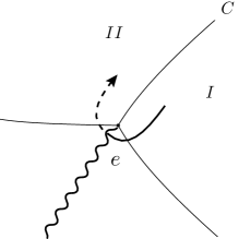
Figure 5.1. The detoured path which encircles the branch point $e$.

Since $e$ is a branch point of the spectral curve, the term-wise analytic continuation of $\psi_{\pm}$ along the detoured path has the phase function with the different sign from the original one. To visualize the two sheets of the spectral curve, we draw the branch cut (the wiggly line) and use the solid (resp., dashed) lines to represent a part of the path on the first (resp., second) sheet. We will use the same rule when we draw paths on the spectral curve.

The connection formula guarantees the single-valuedness of the Borel resummed WKB solutions around branch points (see [91, §6]). We also note that the above formula also has a close relationship to the “path-lifting” in the work of Gaiotto-Moore-Neitzke [33], where Stokes graphs are called spectral networks.

Regarding on the term-wise analytic continuation along the detoured path, we can prove the following (without assuming any conjecture):

Proposition 5.5.

Under the same situation as in Conjecture 5.4, take a point $x_{o}$ on the Stokes curve $C$ and an open neighborhood $U_{o}$ of $x_{o}$ contained in $I\cup C\cup II$. Let $\psi_{\pm}(x,t,\nu;\hbar)$ be the WKB solution defined by (3.30) for $x\in U_{o}$ with the integration path from $0$ to $z(x)$ in (3.30) being chosen as the image by $x\mapsto z(x)$ of the composition of the following two paths on $x$-plane: The part of the Stokes curve $C$ connecting $\infty$ and $x_{o}$, and any path from $x_{o}$ to $x$ contained in $U_{o}$. Then, the term-wise analytic continuation $\tilde{\psi}_{\mp}(x,t,\nu;\hbar)$ of $\psi_{\pm}(x,t,\nu;\hbar)$ along the detoured path encircling $e$ is given by

$$\tilde{\psi}_{\mp}(x,t,\nu;\hbar)=i\cdot(-1)^{m_{C}n_{C}}\cdot\exp\left(\pm\frac{2\pi i{m_{C}}\nu}{\hbar}\right)\cdot\frac{Z(t,\nu\pm n_{C}\hbar;\hbar)}{Z(t,\nu;\hbar)}\cdot\psi_{\mp}(x,t,\nu\pm n_{C}\hbar;\hbar).$$ (5.6)

Here $m_{C}$ and $n_{C}$ are integers defined by the condition

$$\int^{e}_{\infty}\frac{dx}{\sqrt{4x^{3}+2tx+u(t,\nu)}}=\frac{m_{C}\,\omega_{A}+n_{C}\,\omega_{B}}{2},$$ (5.7)

where the left hand-side of (5.7) is defined as the integration along the Stokes curve $C$. (Thus, either $m_{C}$ or $n_{C}$ is an odd integer.)

Proof.

When $x$ turns around $e$ along the detoured path, the function $z(x)$, whose defining path of integration in (3.30) is chosen as the same path for the normalization of $\psi_{\pm}(x,t,\nu;\hbar)$, admits the monodromy

$$z(x)\mapsto-z(x)+m_{C}\,\omega_{A}+n_{C}\,\omega_{B}.$$ (5.8)

Then, the result (5.6) can be proved by a similar computation done in the proof of Theorem 3.9. ∎

5.3. Computation of Stokes multipliers of $(L_{\rm I})$

Assuming Conjectures 5.2 and 5.4 (and the convergence of the Fourier series (4.34) after taking the Borel summation), we demonstrate how the exact WKB method computes the Stokes multipliers of $(L_{\rm I})$. We will apply the Voros connection formula for $\psi_{\pm}$, and take the discrete Fourier transform to compute the Stokes multipliers for $\Psi_{\pm}$.

(a)

(b)

Figure 5.2. (a) The Stokes curves for $t=-9.9313+1.17017i$ and $\nu=1/2$. (b) The anti-Stokes curves for the same $t$ and $\nu$.

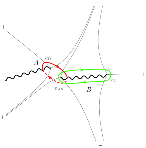
Figure 5.3. The $A$-cycle (red) and the $B$-cycle (green).

We choose $t=-9.9313+1.17017i$ and $\nu=1/2$ for our computation. The (approximated) Stokes graph is shown in Figure 5.2 (a). We also draw the (approximated) anti-Stokes curves, which are defined by the condition ${\rm Re}\int^{x}_{e_{i}}\sqrt{4x^{3}+2tx+u(t,\nu)}\,dx=0$, in Figure 5.2 (b). We can observe that the branch points are connected by the anti-Stokes curves simultaneously; this means that the Boutroux condition

$${\rm Re}\oint_{\gamma}\sqrt{4x^{3}+2tx+u(t,\nu)}\,dx=0\quad\text{for any closed path $\gamma$}$$ (5.9)

is satisfied. We expect that the condition will play a role when we discuss the convergence of 2-parameter solutions. This is the reason why we choose the above parameters $t$ and $\nu$.

After drawing branch cuts (wiggly lines) as in Figure 5.3, we take the branch so that (3.10) holds on the first sheet when $x\to\infty$ with ${\rm Re}\,x>0$. The symbols $\pm$ on the Stokes curves in Figure 5.3 represent the sign of ${\rm Re}\int^{x}_{e_{i}}\sqrt{4x^{3}+2tx+u(t,\nu)}\,dx$ on the Stokes curves. The $A$-cycle and $B$-cycle, which satisfy (3.4) and (3.24) are also indicated in the same figure. We choose the labeling $e_{A},e_{B},e_{AB}$ of the branch points so that the following relations hold modulo $\Lambda$:

$$\int^{e_{A}}_{\infty}\frac{dx}{y}\equiv\frac{\omega_{A}}{2},\quad\int^{e_{B}}_{\infty}\frac{dx}{y}\equiv\frac{\omega_{B}}{2},\quad\int^{e_{AB}}_{\infty}\frac{dx}{y}\equiv\frac{\omega_{A}+\omega_{B}}{2}.$$ (5.10)

There are five asymptotic directions $\arg x=2\ell\pi/5$ ($\ell=0,\pm 1,\pm 2$) of Stokes curves near the infinity. Denote by $s_{\ell}$ ($\ell=0,\pm 1,\pm 2$) the Stokes multipliers of $(L_{\rm I})$ corresponding to these directions, as indicated in Figure 5.4. More precisely, these constants are determined by

$$(\Psi^{(\ell)}_{+},\Psi^{(\ell)}_{-})=\begin{cases}\displaystyle(\Psi^{(\ell+1)}_{+},\Psi^{(\ell+1)}_{-})\cdot\begin{pmatrix}1&0\\ s_{\ell}&1\end{pmatrix}&\quad\text{for $\ell=0,\pm 2$,}\\[15.60007pt] \displaystyle(\Psi^{(\ell+1)}_{+},\Psi^{(\ell+1)}_{-})\cdot\begin{pmatrix}1&s_{\ell}\\ 0&1\end{pmatrix}&\quad\text{for $\ell=\pm 1$,}\end{cases}$$ (5.11)

where

$$\Psi_{\pm}^{(\ell)}=\frac{\sum_{k\in{\mathbb{Z}}}e^{2\pi ik\rho/\hbar}\cdot Z(t,\nu+k\hbar;\hbar)\cdot\psi_{\pm}^{(\ell)}(x,t,\nu+k\hbar;\hbar)}{\sum_{k\in{\mathbb{Z}}}e^{2\pi ik\rho/\hbar}\cdot Z(t,\nu+k\hbar;\hbar)}$$ (5.12)

with $\psi_{\pm}^{(\ell)}$ being the Borel sum of $\psi_{\pm}$ on the Stokes region $\ell$ specified in Figure 5.4. ($Z$ in the right hand-side of (5.12) is also understood to be the Borel sum. We use the same symbol for simplicity.)

To compute $s_{\ell}$, we employ the connection formulas (5.4)-(5.5) and Proposition 5.5. For the convenience, we assign labels to the Stokes curves in Figure 5.4 by the following rule: The Stokes curve $C_{\ast,\ell}$ for $\ast\in\{A,B,AB\}$ and $\ell\in\{0,\pm 1,\pm 2\}$ is the one emanating from the branch point $e_{\ast}$ and flowing to $\infty$ with the asymptotic direction $\arg x=2\ell\pi/5$. The pairs of integers $(m_{C},n_{C})$ which are assigned for the Stokes curves by (5.7) are summarized in Table 5.1. These integers can be computed from the intersection numbers of the detoured path (regarded as a relative homology class on the spectral curve) and the $A$-cycle and $B$-cycle.

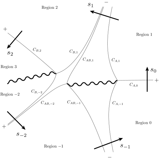
Figure 5.4. The Stokes multipliers of $(L_{\rm I})$ around $x=\infty$.

Stokes curve $C$	$C_{A,0}$	$C_{A,1}$	$C_{A,-1}$	$C_{B,1}$	$C_{B,2}$	$C_{B,-2}$	$C_{AB,1}$	$C_{AB,-1}$	$C_{AB,-2}$
$(m_{C},n_{C})$	$(1,0)$	$(1,0)$	$(1,0)$	$(0,-1)$	$(0,-1)$	$(0,1)$	$(1,-1)$	$(1,1)$	$(1,1)$

Table 5.1. The pair $(m_{C},n_{C})$ for Stokes curves in Figure 5.4.

Under the above preparation, let us compute the Stokes multipliers.

$\bullet$ Computation of $s_{0}$.   Since the sign of the Stokes curve $C_{A,0}$ is plus, the WKB solution $\psi_{+}$ is dominant. Hence, the Voros formula implies

$$\begin{cases}\psi^{(0)}_{+}(x,t,\nu;\hbar)&=\quad\psi^{(1)}_{+}(x,t,\nu;\hbar)+\tilde{\psi}^{(1)}_{-}(x,t,\nu;\hbar)\\[6.00002pt] \psi^{(0)}_{-}(x,t,\nu;\hbar)&=\quad\psi^{(1)}_{-}(x,t,\nu;\hbar).\end{cases}$$ (5.13)

Since $(m_{C_{A,0}},n_{C_{A,0}})=(1,0)$ as shown in Table 5.1, Proposition 5.5 implies that the analytic continuation $\tilde{\psi}_{-}$ along the detoured path encircling $e_{A}$ is given by

$$\tilde{\psi}^{(1)}_{-}(x,t,\nu;\hbar)=i\cdot e^{2\pi i\nu/\hbar}\cdot\psi^{(1)}_{-}(x,t,\nu;\hbar).$$ (5.14)

By shifting $\nu\mapsto\nu+k\hbar$ and taking the discrete Fourier transform, we have

$$\Psi_{+}^{(0)}(x,t,\nu,\rho;\hbar) =\frac{\sum_{k\in{\mathbb{Z}}}e^{2\pi ik\rho/\hbar}\cdot Z(t,\nu+k\hbar;\hbar)\cdot\psi_{+}^{(0)}(x,t,\nu+k\hbar;\hbar)}{\sum_{k\in{\mathbb{Z}}}e^{2\pi ik\rho/\hbar}\cdot Z(t,\nu+k\hbar;\hbar)}$$

$$=\frac{\sum_{k\in{\mathbb{Z}}}e^{2\pi ik\rho/\hbar}\cdot Z(t,\nu+k\hbar;\hbar)\cdot\psi_{+}^{(1)}(x,t,\nu+k\hbar;\hbar)}{\sum_{k\in{\mathbb{Z}}}e^{2\pi ik\rho/\hbar}\cdot Z(t,\nu+k\hbar;\hbar)}$$

$$\quad+\frac{\sum_{k\in{\mathbb{Z}}}e^{2\pi ik\rho/\hbar}\cdot Z(t,\nu+k\hbar;\hbar)\cdot i\cdot e^{2\pi i(\nu+k\hbar)/\hbar}\cdot\psi_{-}^{(1)}(x,t,\nu+k\hbar;\hbar)}{\sum_{k\in{\mathbb{Z}}}e^{2\pi ik\rho/\hbar}\cdot Z(t,\nu+k\hbar;\hbar)}$$

$$=\Psi_{+}^{(1)}(x,t,\nu,\rho;\hbar)+i\cdot e^{2\pi i\nu/\hbar}\cdot\Psi_{-}^{(1)}(x,t,\nu,\rho;\hbar),$$ (5.15)

and

$$\Psi_{-}^{(0)}(x,t,\nu,\rho;\hbar)=\Psi_{-}^{(1)}(x,t,\nu,\rho;\hbar).$$ (5.16)

We have used the periodicity $e^{2\pi i(\nu+k\hbar)/\hbar}=e^{2\pi i\nu/\hbar}$ of the exponential function. From this computation, we conclude

$$s_{0}=i\cdot e^{2\pi i\cdot\nu/\hbar}.$$ (5.17)

$\bullet$ Computation of $s_{-1}$. In this case, we need to cross two Stokes curves $C_{AB,-1}$ and $C_{A,-1}$ passing an intermediate Stokes region between them. Both Stokes curves have the minus sign, so the WKB solution $\psi_{-}$ is dominant.

Let us denote by $\psi_{\pm}^{(-1/2)}$ the Borel sum of the WKB solution $\psi_{\pm}$ on the intermediate Stokes region. Then, the Voros formula and Proposition 5.5 imply

$$\begin{cases}\psi^{(-1)}_{+}(x,t,\nu;\hbar)&=\quad\psi^{(-1/2)}_{+}(x,t,\nu;\hbar)\\[6.00002pt] \psi^{(-1)}_{-}(x,t,\nu;\hbar)&=\quad\psi^{(-1/2)}_{-}(x,t,\nu;\hbar)+\tilde{\psi}^{(-1/2)}_{+}(x,t,\nu;\hbar)\end{cases}$$ (5.18)

holds on the Stokes curve $C_{AB,-1}$ with

$$\tilde{\psi}^{(-1/2)}_{+}(x,t,\nu;\hbar)=-i\cdot e^{-2\pi i\nu/\hbar}\cdot\frac{Z(t,\nu-\hbar;\hbar)}{Z(t,\nu;\hbar)}\cdot\psi^{(-1/2)}_{+}(x,t,\nu-\hbar;\hbar).$$ (5.19)

Similarly, on the Stokes curve $C_{A,-1}$, we have

$$\begin{cases}\psi^{(-1/2)}_{+}(x,t,\nu;\hbar)&=\quad\psi^{(0)}_{+}(x,t,\nu;\hbar)\\[6.00002pt] \psi^{(-1/2)}_{-}(x,t,\nu;\hbar)&=\quad\psi^{(0)}_{-}(x,t,\nu;\hbar)+\tilde{\psi}^{(0)}_{+}(x,t,\nu;\hbar)\end{cases}$$ (5.20)

with

$$\tilde{\psi}^{(0)}_{+}(x,t,\nu;\hbar)=i\cdot e^{-2\pi i\nu/\hbar}\cdot\psi^{(0)}_{+}(x,t,\nu;\hbar).$$ (5.21)

Summarizing these formulas, we have

$$\psi^{(-1)}_{+}(x,t,\nu;\hbar) =\psi^{(0)}_{+}(x,t,\nu;\hbar)$$ (5.22)

$$\psi^{(-1)}_{-}(x,t,\nu;\hbar) =\psi^{(0)}_{-}(x,t,\nu;\hbar)-i\cdot e^{-2\pi i\nu/\hbar}\cdot\frac{Z(t,\nu-\hbar;\hbar)}{Z(t,\nu;\hbar)}\cdot\psi^{(0)}_{+}(x,t,\nu-\hbar;\hbar)$$

$$\qquad+i\cdot e^{-2\pi i\nu/\hbar}\cdot\psi^{(0)}_{+}(x,t,\nu;\hbar).$$ (5.23)

Again, by taking the discrete Fourier transform, we have

$$\Psi^{(-1)}_{+}(x,t,\nu,\rho;\hbar)=\Psi^{(0)}_{+}(x,t,\nu,\rho;\hbar)$$ (5.24)

and

$$\Psi^{(-1)}_{-}(x,t,\nu,\rho;\hbar) =\frac{\sum_{k\in{\mathbb{Z}}}e^{2\pi ik\rho/\hbar}\cdot Z(t,\nu+k\hbar;\hbar)\cdot\psi_{-}^{(0)}(x,t,\nu+k\hbar;\hbar)}{\sum_{k\in{\mathbb{Z}}}e^{2\pi ik\rho/\hbar}\cdot Z(t,\nu+k\hbar;\hbar)}$$

$$\quad-\frac{\sum_{k\in{\mathbb{Z}}}e^{2\pi ik\rho/\hbar}\cdot Z(t,\nu+k\hbar-\hbar;\hbar)\cdot i\cdot e^{-2\pi i(\nu+k\hbar)/\hbar}\cdot\psi_{+}^{(0)}(x,t,\nu+k\hbar-\hbar;\hbar)}{\sum_{k\in{\mathbb{Z}}}e^{2\pi ik\rho/\hbar}\cdot Z(t,\nu+k\hbar;\hbar)}$$

$$\quad+\frac{\sum_{k\in{\mathbb{Z}}}e^{2\pi ik\rho/\hbar}\cdot Z(t,\nu+k\hbar;\hbar)\cdot i\cdot e^{-2\pi i(\nu+k\hbar)/\hbar}\cdot\psi_{+}^{(0)}(x,t,\nu+k\hbar;\hbar)}{\sum_{k\in{\mathbb{Z}}}e^{2\pi ik\rho/\hbar}\cdot Z(t,\nu+k\hbar;\hbar)}$$

$$=\Psi^{(0)}_{-}(x,t,\nu,\rho;\hbar)+i\cdot(-e^{-2\pi i(\nu-\rho)/\hbar}+e^{-2\pi i\nu/\hbar})\cdot\Psi^{(0)}_{+}(x,t,\nu,\rho;\hbar).$$ (5.25)

Thus we have

$$s_{-1}=i\cdot(-e^{-2\pi i(\nu-\rho)/\hbar}+e^{-2\pi i\nu/\hbar}).$$ (5.26)

$\bullet$ Computation of other Stokes multipliers.   The above computations imply that the Voros formulas and Proposition 5.5 are enough to calculate the Stokes multipliers. The general formula is given as follows:

$$s_{\ell}=i\cdot\sum_{C}\,(-1)^{m_{C}n_{C}}\cdot e^{{\rm sign}(C)\cdot 2\pi i(m_{C}\nu-n_{C}\rho)/\hbar}.$$ (5.27)

Here the summation is taken over all Stokes curves which have $\arg x=2\ell\pi/5$ as the asymptotic direction, and ${\rm sign}(C)\in\{\pm 1\}$ is the sign for the Stokes curve $C$ which specifies the dominant WKB solution on $C$. In summary, we have the following table of the Stokes multipliers in Figure 5.4:

$$\begin{cases}s_{-2}=i\cdot(e^{-2\pi i\rho/\hbar}-e^{2\pi i(\nu-\rho)/\hbar}),\\ s_{-1}=i\cdot(-e^{-2\pi i(\nu-\rho)/\hbar}+e^{-2\pi i\nu/\hbar}),\\ s_{0}\hskip 7.20009pt=i\cdot e^{2\pi i\nu/\hbar},\\ s_{1}\hskip 7.20009pt=i\cdot(e^{-2\pi i\nu/\hbar}-e^{-2\pi i(\nu+\rho)/\hbar}+e^{-2\pi i\rho/\hbar}),\\ s_{2}\hskip 7.20009pt=i\cdot e^{2\pi i\rho/\hbar}.\end{cases}$$ (5.28)

Let us give two remarks. First, the Stokes multipliers we have computed are independent of $t$. This is consistent with the fact that $\Psi_{\pm}$ satisfies the isomonodromy system $(L_{\rm I})$-$(D_{\rm I})$ given in (2.12)-(2.13). Second, $s_{\ell}$’s satisfy the cyclic relation:

$$\begin{pmatrix}1&0\\ s_{2}&1\end{pmatrix}\cdot\begin{pmatrix}1&s_{1}\\ 0&1\end{pmatrix}\cdot\begin{pmatrix}1&0\\ s_{0}&1\end{pmatrix}\cdot\begin{pmatrix}1&s_{-1}\\ 0&1\end{pmatrix}\cdot\begin{pmatrix}1&0\\ s_{-2}&1\end{pmatrix}=\begin{pmatrix}0&i\\ i&0\end{pmatrix}.$$ (5.29)

In other words, they satisfy the relations

$$1+s_{\ell-1}\cdot s_{\ell}+i\cdot s_{\ell+2}=0,\quad s_{\ell+5}=s_{\ell},$$ (5.30)

which are essentially the cluster exchange relations in the $A_{2}$ cluster algebra, or the defining equation of the monodromy space, or the wild character variety (c.f., [31, 81]). These are supporting evidence for the validity of our computation.

6. Conclusion and open problems

In this article, we have constructed a 2-parameter family of (formal) $\tau$-function for the first Painlevé equation $(P_{\rm I})$ as the discrete Fourier transform of the topological recursion partition function applied to a family of genus $1$ spectral curves. We also obtained a solution of isomonodromy system associated with $(P_{\rm I})$ with the aid of techniques used in literature of quantum curves.

We summarize several questions and open problems in the following list.

1. We expect that the results obtained in this paper for Painlevé I can be generalized to other Painlevé equations including a class of higher order analogues. The Fourier series structure also appears in the higher order Painlevé equations (see [36, 37] for example). In a recent article [69] by Marchal-Orantin, a systematic approach to rank 2 isomonodromy systems via the topological recursion is established. These works seem to be good references for the direction.

2. Aoki-Kawai-Takei also constructed a 2-parameter family of WKB-theoretic formal solutions of Painlevé equations ([5]); see also [2, 40, 93] for $\hbar=1$ case. More generally, full-parameter formal solutions are also constructed for a class of higher order Painlevé equations (Painlevé hierarchies) in [3] etc. Their solution contains infinitely many exponential terms, but it is not directly related to $\theta$-functions or elliptic functions. It is interesting to find a relationship between our 2-parameter solution and theirs.

   Kawai-Takei also introduced the notion of (non-linear version of) turning points and Stokes curves for the Painlevé equations in [61], and proved that their 2-parameter formal solution of Painlevé II – VI can be reduced to that of Painlevé I near each simple turning point by a certain change of variables ([61, 62]; see also [47]). These results should have a counterpart in the framework developed in this paper.

3. The computational method of the Stokes multipliers presented in §5 contains several heuristic arguments: Borel summability of the WKB series, Voros connection formulas, convergence of the Fourier series, are the open problems to be solved.

   Borel summability is proved for some special cases: Kamimoto-Koike ([58]) proved the Borel summability of $0$-parameter solutions of classical six Painlevé equations on compliments of Stokes curves in the sense of Kawai-Takei ([61]). See also the work by Costin ([21]) which includes the Borel summability of $1$-parameter (trans-series solution) of Painlevé equations with $\hbar=1$.

   Moreover, in articles [2, 23, 31, 59, 60, 68, 89] etc., connection problem (non-linear Stokes phenomenon) of Painlevé equations are discussed. Our approach to the direct monodromy problem should be compared to the previous results.

4. The Stokes graphs and trajectories of quadratic differentials are also used in the study of the space of Bridgeland stability conditions ([14]) for a class of Calabi-Yau 3 categories of quiver representations ([15]). In [87] and [88], Sutherland studied the stability conditions for a class of quivers, called “Painlevé quivers”. In the case of Painlevé I, the relevant quadratic differential is equivalent to the one used in §5 (whose associated quiver is of type $A_{2}$). In this picture, the variation of $t$ (i.e., deformation of the spectral curve) is related to the variation of stability conditions. It seems to be interesting to investigate a relationship between the analytic continuation of Painlevé transcendents and the variation of stability conditions (wall-crossings) for the corresponding Painlevé quivers. The work [68] by Lisovyy-Roussillon pointed that the dilogarithm identity appears as a consistency condition in the connection problem for Painlevé I.

5. In the ($c=1$ Virasoro) conformal field theoretic construction of $\tau$-function for Painlevé VI by Gamayun-Iorgov-Lisovyy ([34]), the expansion coefficients of 2-parameter $\tau$-function are described by an explicit and combinatorial formula, thanks to the AGT correspondence [1] and Nekrasov’ formula [75]. In the works [38, 39] of Gavrylenko-Lisovyy, the same explicit formulas for Painlevé VI and III are obtained through an explicit calculation of the Fredholm determinant for the associated Riemann-Hilbert problem (see also [16]). It would be great if we obtain such an explicit formula for Painlevé I.

6. Conjectural expressions of 2-parameter $\tau$-functions for Painlevé II – Painlevé V as the discrete Fourier transform of irregular conformal blocks are discussed by the works [71, 72] of Nagoya. However, finding such an expression is an open problem for Painlevé I case.

7. Theorem 4.3 shows in particular that our formal $\tau$-function (4.1) satisfies the Hirota-type bilinear identity (2.8). In [6, 7], Bershtein-Shchechkin gave an interesting observation; the Hirota-type identities arising from a class of ($q$-)Painlevé equations can be interpreted as the Nakajima-Yoshioka’s blow-up equation ([73, 74]). It seems to be interesting to give such an interpretation (from the instanton counting) for the Hirota-type equation (2.8).

Appendix A Weierstrass functions and $\theta$-functions

Here we summarize properties of Weierstrass elliptic functions and $\theta$-functions which are relevant in this paper. See [92] for more details.

A.1. Weierstrass functions

A.1.1. Weierstrass $\wp$-function

Let

$$\omega_{A}:=\oint_{A}\frac{dx}{\sqrt{4x^{3}-g_{2}x-g_{3}}},\quad\omega_{B}:=\oint_{B}\frac{dx}{\sqrt{4x^{3}-g_{2}x-g_{3}}}$$ (A.1)

be the periods of smooth elliptic curve $\Sigma$ defined by $y^{2}=4x^{3}-g_{2}x-g_{3}$. Here ${A},{B}$ are generators of the first homology group $H_{1}(\Sigma,{\mathbb{Z}})$. We assume that $\tau:=\omega_{B}/\omega_{A}$ has a positive imaginary part. The coefficients $g_{2}$, $g_{3}$ are related to these periods by

$$g_{2}=60\sum_{\omega\in\Lambda\setminus\{0\}}\frac{1}{\omega^{4}},\qquad g_{3}=140\sum_{\omega\in\Lambda\setminus\{0\}}\frac{1}{\omega^{6}}.$$ (A.2)

Here $\Lambda={\mathbb{Z}}\cdot\omega_{A}+{\mathbb{Z}}\cdot\omega_{B}$ be the lattice generated by the two complex numbers $\omega_{A}$ and $\omega_{B}$.

Under the notations, the Weierstrass elliptic function $\wp(z)(=\wp(z;g_{2},g_{3}))$ is defined by

$$\wp(z):=\frac{1}{z^{2}}+\sum_{\omega\in\Lambda\setminus\{0\}}\left(\frac{1}{(z-\omega)^{2}}-\frac{1}{\omega^{2}}\right).$$ (A.3)

It is also constructed as the inverse function of the elliptic integral

$$z(x):=\int^{x}_{\infty}\frac{dx}{\sqrt{4x^{3}-g_{2}x-g_{3}}},$$ (A.4)

and hence $\wp(z)$ is doubly-periodic function with periods $\omega_{A}$ and $\omega_{B}$. It has double pole at $z=m\,\omega_{A}+n\,\omega_{B}$ for any $(m,n)\in{\mathbb{Z}}^{2}$. We also note that $\wp(z)$ is an even function; that is $\wp(-z)=\wp(z)$.

The Weierstarss $\wp$-function satisfies the following non-linear ODE:

$$\left(\frac{d\wp}{dz}(z)\right)^{2}=4\wp(z)^{3}-g_{2}\,\wp(z)-g_{3}.$$ (A.5)

Thus the $\wp$-function is used to parametrize elliptic curves. Moreover, differentiating the relation, we also have

$$\frac{d^{2}\wp}{dz^{2}}(z)=6\wp(z)^{2}-\frac{g_{2}}{2}.$$ (A.6)

A.1.2. Weierstrass $\zeta$-function

We also introduce the Weierstrass $\zeta$-function

$$\zeta(z):=\frac{1}{z}+\sum_{\omega\in\Lambda\setminus\{0\}}\left(\frac{1}{z-\omega}+\frac{1}{\omega}+\frac{z}{\omega^{2}}\right),$$ (A.7)

which satisfies $-\zeta^{\prime}(z)=\wp(z)$. The function $\zeta(z)$ is not doubly-periodic, but it satisfies

$$\zeta(z+m\,\omega_{A}+n\,\omega_{B})=\zeta(z)+m\,\eta_{A}+n\,\eta_{B}\quad(m,n\in{\mathbb{Z}}).$$ (A.8)

The constants $\eta_{A}$ and $\eta_{B}$ are also expressed as elliptic integral (of the second kind):

$$\eta_{\ast}:=-\oint_{\ast}\frac{xdx}{\sqrt{4x^{3}-g_{2}x-g_{3}}}=\frac{1}{2}\,\zeta\left(\frac{\omega_{\ast}}{2}\right)\quad(\ast\in\{A,B\}).$$ (A.9)

The Riemann bilinear identity shows

$$\eta_{A}\cdot\omega_{B}-\eta_{B}\cdot\omega_{A}=2\pi i.$$ (A.10)

A.1.3. Weierstrass $\sigma$-function

The integral of the Weierstrass zeta function is expressed as the logarithm of the Weierstrass $\sigma$-function defined by

$$\sigma(z):=z\cdot\prod_{\omega\in\Lambda\setminus\{0\}}\left(1-\frac{z}{\omega}\right)\cdot\exp\left(\frac{z}{\omega}+\frac{z^{2}}{2\omega^{2}}\right).$$ (A.11)

This satisfies $d\log\sigma(z)/dz=\zeta(z)$. $\sigma$-function possesses the following quasi-periodicity:

$$\sigma(z+m\,\omega_{A}+n\,\omega_{B})=(-1)^{m+n+mn}\cdot\exp\left((m\,\eta_{A}+n\,\eta_{B})\cdot\Bigl{(}z+\frac{m\,\omega_{A}+n\,\omega_{B}}{2}\Bigr{)}\right)\cdot\sigma(z)\quad(m,n\in{\mathbb{Z}}).$$ (A.12)

It is also known that the $\sigma$-function also satisfies the addition formula:

$$\frac{\sigma(z+w)\cdot\sigma(z-w)}{\sigma(z)^{2}\cdot\sigma(w)^{2}}=\wp(w)-\wp(z).$$ (A.13)

A.2. $\theta$-functions

The Riemann $\theta$-function is defined by

$$\theta(v,\tau):=\sum_{k\in{\mathbb{Z}}}e^{2\pi ikv+\pi ik^{2}\tau}.$$ (A.14)

This is known to convergent uniformly on $(v,\tau)\in{\mathbb{C}}\times{\mathbb{H}}$. We also use the $\theta$-functions with characteristics:

$$\theta_{00}(v,\tau):=\theta(v,\tau) =\sum_{k\in{\mathbb{Z}}}e^{2\pi ikv+\pi k^{2}\tau}$$ (A.15)

$$\theta_{01}(v,\tau) :=\sum_{k\in{\mathbb{Z}}}e^{2\pi ik\bigl{(}v+\frac{1}{2}\bigr{)}+\pi k^{2}\tau}$$ (A.16)

$$\theta_{10}(v,\tau) :=\sum_{k\in{\mathbb{Z}}}e^{2\pi i\bigl{(}k+\frac{1}{2}\bigr{)}v+\pi\bigl{(}n+\frac{1}{2}\bigr{)}^{2}\tau}$$ (A.17)

$$\theta_{11}(v,\tau) :=\sum_{k\in{\mathbb{Z}}}e^{2\pi i\bigl{(}k+\frac{1}{2}\bigr{)}\bigl{(}v+\frac{1}{2}\bigr{)}+\pi\bigl{(}k+\frac{1}{2}\bigr{)}^{2}\tau}.$$ (A.18)

The parity of these functions are

$$\theta_{00}(-v,\tau)=\theta_{00}(v,\tau),\quad\theta_{01}(-v,\tau)=\theta_{01}(v,\tau),\quad\theta_{10}(-v,\tau)=\theta_{10}(v,\tau),\quad\theta_{11}(-v,\tau)=-\theta_{11}(v,\tau).$$ (A.19)

The relation to the Weierstrass $\sigma$-function is given as

$$\sigma(z)=\exp\left(\frac{\eta_{A}}{2\omega_{A}}\cdot z^{2}\right)\cdot\frac{\omega_{A}}{\theta_{11}^{\prime}(0,\tau)}\cdot\theta_{11}\left(\frac{z}{\omega_{A}},\tau\right).$$ (A.20)

By taking the logarithm derivative, we have

$$\wp(z)=-\frac{\eta_{A}}{\omega_{A}}-\frac{1}{\omega_{A}^{2}}\cdot\left[\frac{\partial^{2}}{\partial v^{2}}\log\theta_{11}(v,\tau)\right]_{v=\frac{z}{\omega_{A}}}=-\frac{\eta_{A}}{\omega_{A}}-\frac{1}{\omega_{A}^{2}}\cdot\left[\frac{\partial^{2}}{\partial v^{2}}\log\theta_{00}(v,\tau)\right]_{v=\frac{z}{\omega_{A}}-\frac{1}{2}-\frac{\tau}{2}}.$$ (A.21)

The last equality follows from the relation

$$\theta_{00}(v,\tau)=-e^{\pi iv+\frac{i\pi\tau}{4}}\cdot\theta_{11}\Bigl{(}v+\frac{1}{2}+\frac{\tau}{2},\tau\Bigr{)}.$$ (A.22)

Appendix B Proof of Theorem 3.7

Here we give a proof of Theorem 3.7 which plays an important role in the proof of our main result. We use the same notation used in §3.2.3. (For example, the symbol $z_{[\hat{j}]}$ for $j=1,\dots,n$ means the $(n-1)$-tuple of variables $(z_{1},\dots,\hat{z}_{j},\dots,z_{n})$ without $j$-th entry.)

Lemma B.1.

The function $F_{g,n}(z_{1},\dots,z_{n})$ defined in (3.39) satisfies the following equality for $2g-2+n\geq 1$:

$$\frac{\partial F_{g,n}}{\partial z_{1}}(z_{1},\dots,z_{n})=G_{g,n}(z_{1},\dots,z_{n})-\frac{1}{\omega_{A}}\oint_{z\in A}\frac{R_{g,n}(z,z_{2},\dots,z_{n})}{(y(z)-y(\bar{z}))\cdot dx(z)},$$ (B.1)

with $G_{g,n}$ and $R_{g,n}$ being given as follows:

• For $2g-2+n=1$, we set

  $$G_{0,3}(z_{1},z_{2},z_{3}) :=-\sum_{j=2}^{3}\bigl{(}P(z_{1}+z_{j})-P(z_{1}-z_{j})\bigr{)}$$

  $$\qquad\times\biggl{(}\frac{1}{2y(z_{1})\cdot\frac{dx}{dz}(z_{1})}\cdot\frac{\partial F_{0,2}}{\partial z_{1}}(z_{[\hat{j}]})-\frac{1}{2y(z_{j})\cdot\frac{dx}{dz}(z_{j})}\cdot\frac{\partial F_{0,2}}{\partial z_{j}}(z_{[\hat{1}]})\biggr{)}$$

  $$\quad+\frac{1}{y(z_{1})\cdot\frac{dx}{dz}(z_{1})}\cdot\frac{\partial F_{0,2}}{\partial z_{1}}(z_{1},z_{2})\cdot\frac{\partial F_{0,2}}{\partial z_{1}}(z_{1},z_{3}),$$ (B.2)

  $$G_{1,1}(z_{1}) :=-\frac{1}{2y(z_{1})\cdot\frac{dx}{dz}(z_{1})}\cdot\frac{\partial^{2}}{\partial u_{1}\partial u_{2}}F_{0,2}(u_{1},u_{2})\biggl{|}_{u_{1}=u_{2}=z_{1}},$$ (B.3)

  with $P(z)$ being given in (3.13), and for $2g-2+n\geq 2$, we set

  $$G_{g,n}(z_{1},\dots,z_{n})$$

  $$\quad:=-\sum_{j=2}^{n}\bigl{(}P(z_{1}+z_{j})-P(z_{1}-z_{j})\bigr{)}$$

  $$\qquad\times\biggl{(}\frac{1}{2y(z_{1})\cdot\frac{dx}{dz}(z_{1})}\cdot\frac{\partial F_{g,n-1}}{\partial z_{1}}(z_{[\hat{j}]})-\frac{1}{2y(z_{j})\cdot\frac{dx}{dz}(z_{j})}\cdot\frac{\partial F_{g,n-1}}{\partial z_{j}}(z_{[\hat{1}]})\biggr{)}$$

  $$\qquad-\frac{1}{2y(z_{1})\cdot\frac{dx}{dz}(z_{1})}\cdot\frac{\partial^{2}}{\partial u_{1}\partial u_{2}}\biggl{(}F_{g-1,n+1}(u_{1},u_{2},z_{[\hat{1}]})$$

  $$\hskip 120.0003pt+\sum_{\begin{subarray}{c}g_{1}+g_{2}=g\\ I\sqcup J=[\hat{1}]\end{subarray}}^{\rm stable}F_{g_{1},|I|+1}(u_{1},z_{I})\cdot F_{g_{2},|J|+1}(u_{2},z_{J})\biggr{)}\Biggr{|}_{u_{1}=u_{2}=z_{1}}.$$ (B.4)

• $R_{g,n}(z,z_{2},\dots,z_{n})$ is a quadratic differential in the variable $z$ (and functions of other variables $z_{2},\dots,z_{n}$) defined by

  $$R_{0,3}(z,z_{2},z_{3}) :=\biggl{(}\int^{z_{2}}_{0}W_{0,2}(z,z_{2})\biggr{)}\cdot\biggl{(}\int^{z_{3}}_{0}W_{0,2}(\bar{z},z_{3})\biggr{)}$$

  $$\qquad+\biggl{(}\int^{z_{3}}_{0}W_{0,2}(z,z_{3})\biggr{)}\cdot\biggl{(}\int^{z_{2}}_{0}W_{0,2}(\bar{z},z_{2})\biggr{)},$$ (B.5)

  $$R_{1,1}(z) :=W_{0,2}(z,\bar{z}),$$ (B.6)

  for $2g-2+n=1$, and

  $$R_{g,n}(z,z_{2},\dots,z_{n})$$

  $$:=\sum_{j=2}^{n}\Biggl{[}\biggl{(}\int^{z_{j}}_{0}W_{0,2}(z,z_{j})\biggr{)}\cdot\biggl{(}\int^{z_{[\hat{1},\hat{j}]}}_{0}W_{g,n-1}(\bar{z},z_{[\hat{1},\hat{j}]})\biggr{)}$$

  $$\hskip 84.00021pt+\biggl{(}\int^{z_{j}}_{0}W_{0,2}(\bar{z},z_{j})\biggr{)}\cdot\biggl{(}\int^{z_{[\hat{1},\hat{j}]}}_{0}W_{g,n-1}(z,z_{[\hat{1},\hat{j}]})\biggr{)}\Biggr{]}$$

  $$\quad+\int^{z_{[\hat{1}]}}_{0}W_{g-1,n+1}(z,\bar{z},z_{[\hat{1}]})+\sum_{\begin{subarray}{c}g_{1}+g_{2}=g\\ I\sqcup J=[\hat{1}]\end{subarray}}^{\text{\rm stable}}\biggl{(}\int^{z_{I}}_{0}W_{g_{1},|I|+1}(z,z_{I})\biggr{)}\cdot\biggl{(}\int^{z_{J}}_{0}W_{g_{2},|J|+1}(\bar{z},z_{J})\biggr{)}$$

  for $2g-2+n\geq 2$. Here, for a set $L=\{\ell_{1},\dots,\ell_{k}\}\subset\{1,\dots,n\}$ of indices, we have used the notation

  $$\int^{z_{L}}_{0}W_{g,n}(z_{1},\dots,z_{n}):=\int^{z_{\ell_{1}}}_{0}\cdots\int^{z_{\ell_{k}}}_{0}W_{g,n}(z_{1},\dots,z_{n}).$$ (B.8)

Proof.

First we show the claim in the case $2g-2+n\geq 2$. We employ a similar technique used in the proof of [54, Theorem 3.11].

Integrating the topological recursion relation (3.15) with respect to $z_{2},\dots,z_{n}$, we have

$$\frac{\partial}{\partial z_{1}}F_{g,n}(z_{1},\dots,z_{n})\,dz_{1} =\int_{0}^{z_{2}}\cdots\int_{0}^{z_{n}}W_{g,n}(z_{1},z_{2},\dots,z_{n})$$

$$=\frac{1}{2\pi i}\sum_{j=1}^{3}\oint_{\gamma_{j}}K(z_{1},z)\cdot R_{g,n}(z,z_{1},\dots,z_{n}).$$ (B.9)

Note that, as a differential of $z$, $R_{g,n}$ has a simple pole at $z\equiv z_{1},\bar{z}_{1},\dots,z_{n},\bar{z}_{n}$ modulo $\Lambda$, and no other poles except for the ramification points. Hence, the residue theorem implies

$$\frac{\partial}{\partial z_{1}}F_{g,n}(z_{1},\dots,z_{n})\,dz_{1}$$

$$=-\sum_{i=1}^{n}\sum_{p=z_{i},\bar{z}_{i}}\mathop{\rm Res}_{z=p}K(z_{1},z)\cdot R_{g,n}(z,z_{2},\dots,z_{n})+\frac{1}{2\pi i}\oint_{z\in\partial D}K(z_{1},z)\cdot R_{g,n}(z,z_{2},\dots,z_{n})$$

$$=\sum_{i=1}^{n}\sum_{p=z_{i},\bar{z}_{i}}\mathop{\rm Res}_{z=p}\frac{P(z_{1}+z)-P(z_{1}-z)}{4y(z)\cdot dx(z)}\cdot\Biggl{(}\sum_{j=2}^{n}\Biggl{[}\Bigl{(}P_{1}(z+z_{j})-P_{1}(z-z_{j})\Bigr{)}\cdot\frac{\partial}{\partial u}F_{g,n-1}(u,z_{[\hat{1},\hat{j}]})\Biggr{]}\Biggl{|}_{u=z}$$

$$\quad+\frac{\partial^{2}}{\partial u_{1}\partial u_{2}}\biggl{[}F_{g-1,n+1}(u_{1},u_{2},z_{[\hat{1}]})+\sum_{\begin{subarray}{c}g_{1}+g_{2}=g\\ I\sqcup J=[\hat{1}]\end{subarray}}^{\text{stable}}F_{g_{1},|I|+1}(u_{1},z_{I})\cdot F_{g_{2},|J|+1}(u_{2},z_{J})\biggr{]}\Biggl{|}_{u_{1}=u_{2}=z}\Biggr{)}\,dz_{1}$$

$$\quad+\frac{1}{2\pi i}\oint_{z\in\partial\Omega}K(z_{1},z)\cdot R_{g,n}(z,z_{2},\dots,z_{n}).$$ (B.10)

The last term is the integration along the boundary of the fundamental domain $\Omega$ of the elliptic curve.

The first two lines of the right hand-side of (B.10) coincides with $G_{g,n}(z_{1},\dots,z_{n})$ in the desired equality (B.1) (c.f., [26, Theorem 4.7]). On the other hand, since

$$K(z_{1},z+\omega_{\ast})-K(z_{1},z)=\begin{cases}0&\text{for $\ast=A$}\\ \displaystyle\frac{1}{(y(z)-y(\bar{z}))\cdot dx(z)}\cdot\frac{2\pi i}{\omega_{A}}\cdot dz_{1}&\text{for $\ast=B$},\end{cases}$$ (B.11)

the integration along $\partial\Omega$ is computed as follows:

$$\frac{1}{2\pi i}\int_{z\in\partial D}K(z_{1},z)\cdot R_{g,n}(z,z_{2},\dots,z_{n})$$ (B.12)

$$\quad=\frac{1}{2\pi i}\int_{z\in A}(K(z_{1},z)-K(z_{1},z+\omega_{B}))\cdot R_{g,n}(z,z_{2},\dots,z_{n})$$ (B.13)

$$\qquad-\frac{1}{2\pi i}\int_{z\in B}(K(z_{1},z)-K(z_{1},z+\omega_{A}))\cdot R_{g,n}(z,z_{2},\dots,z_{n})$$ (B.14)

$$\quad=-\frac{dz_{1}}{\omega_{A}}\oint_{z\in A}\frac{R_{g,n}(z,z_{2},\dots,z_{n})}{(y(z)-y(\bar{z}))\cdot dx(z)}.$$ (B.15)

Thus we have proved (B.1) for $2g-2+n\geq 2$.

The exceptional two cases $(g,n)=(0,3)$ and $(1,1)$ can be checked similarly by using the identity

$$\frac{\partial}{\partial z_{1}}F_{0,2}(z_{1},z_{2})\cdot dz_{1}=\bigl{(}P(z_{1}+z_{2})-P(z_{1})\bigr{)}\cdot dz_{1}=-\int^{z_{2}}_{0}W_{0,2}(\bar{z}_{1},z_{2})$$ (B.16)

which immediately follows from the definition (3.34) of $F_{0,2}$. ∎

The following formula will be used to relate the $A$-cycle integral in the right hand-side of (B.1) with the $t$-derivatives.

Lemma B.2.

For $2g-2+n\geq 1$, we have

$$\frac{\partial}{\partial t}F_{g,n-1}(z(x_{1}),\dots,z(x_{n-1}))=E_{g,n-1}(z(x_{1}),\dots,z(x_{n-1})),$$ (B.17)

where

$$E_{g,n-1}(z_{1},\dots,z_{n-1})$$

$$\quad:=-\frac{1}{\omega_{A}}\oint_{z\in A}\frac{R_{g,n}(z,z_{1},\dots,z_{n-1})}{(y(z)-y(\bar{z}))\cdot dx(z)}+\sum_{j=1}^{n-1}\frac{P(z_{j})}{y(z_{j})\cdot\frac{dx}{dz}(z_{j})}\cdot\frac{\partial F_{g,n-1}}{\partial z_{j}}(z_{1},\dots,z_{n-1}).$$ (B.18)

Proof.

Replacing the label $z_{1}\leftrightarrow z_{n}$ in (B.1) and taking the following residue around $z_{n}=0$, we have

$$\mathop{\rm Res}_{z_{n}=0}\left(z_{n}^{-1}\cdot\frac{\partial F_{g,n}}{\partial z_{n}}(z_{1},\dots,z_{n})\cdot dz_{n}\right)\\ =-\frac{1}{\omega_{A}}\oint_{z\in A}\frac{R_{g,n}(z,z_{1},\dots,z_{n-1})}{(y(z)-y(\bar{z}))dx(z)}+\sum_{j=1}^{n-1}\frac{P(z_{j})}{y(z_{j})\cdot\frac{dx}{dz}(z_{j})}\cdot\frac{\partial F_{g,n-1}}{\partial z_{j}}(z_{1},\dots,z_{n-1}).$$ (B.19)

Proposition 3.4 shows that the left hand-side is nothing but the $t$-derivation of $F_{g,n-1}$, if we use the $x$-coordinates. This completes the proof. ∎

Let us set $\tilde{G}_{g,n}(z_{1},\dots,z_{n}):=\partial_{z_{1}}F_{g,n}(z_{1},\dots,z_{n})-G_{g,n}(z_{1},\dots,z_{n})$. By a similar computation in [26, Theorem 6.5], we have

$$\sum_{\begin{subarray}{c}g\geq 0,~{}n\geq 1\\ 2g-2+n=m\end{subarray}}\left[\frac{2\tilde{G}_{g,n}(z_{1},\dots,z_{n})}{{(n-1)!}}\right]_{z_{1}=\cdots=z_{n}=z(x)}$$

$$\quad=\begin{cases}\displaystyle 2y\bigl{(}z(x)\bigr{)}\cdot\frac{\partial S_{m}(x)}{\partial x}+\left(-\frac{\partial_{x}y\bigl{(}z(x)\bigr{)}}{y\bigl{(}z(x)\bigr{)}}\right)\cdot\frac{\partial S_{m-1}(x)}{\partial x}&\\[18.00005pt] \hskip 60.00015pt\displaystyle+\sum_{\begin{subarray}{c}m_{1},m_{2}\geq 1\\ m_{1}+m_{2}=m-1\end{subarray}}\frac{\partial S_{m_{1}}(x)}{\partial x}\cdot\frac{\partial S_{m_{2}}(x)}{\partial x}+\frac{\partial^{2}S_{m-1}(x)}{\partial x^{2}}&\quad\text{for $m\geq 2$}\\[30.00008pt] \displaystyle 2y\bigl{(}z(x)\bigr{)}\cdot\frac{\partial S_{1}(x)}{\partial x}+\left(-\frac{\partial_{x}y\bigl{(}z(x)\bigr{)}}{y\bigl{(}z(x)\bigr{)}}\right)\cdot\frac{\partial S_{0}(x)}{\partial x}-\left(\frac{\partial S_{0}(x)}{\partial x}\right)^{2}+\frac{\partial^{2}S_{0}(x)}{\partial x^{2}}&\quad\text{for $m=1$}.\end{cases}$$ (B.20)

(Recall that $S_{m}(x)$’s are defined in §3.4.) Here we have used the identity $y\bigl{(}z(x)\bigr{)}=\frac{dx}{dz}\bigl{(}z(x)\bigr{)}$.

Next, using Lemma B.1 and Lemma B.2, let us find another expression of the left hand-side of (B.20). First, we note

$$\sum_{\begin{subarray}{c}g\geq 0,~{}n\geq 1\\ 2g-2+n=m\end{subarray}}\left[\frac{2\tilde{G}_{g,n}(z_{1},\dots,z_{n})}{{(n-1)!}}\right]_{z_{1}=\cdots=z_{n}=z(x)}$$

$$=\sum_{\begin{subarray}{c}g\geq 0,~{}n\geq 1\\ 2g-2+n=m\end{subarray}}\left[\frac{2\tilde{G}_{g,n}(z_{1},\dots,z_{n})}{{(n-1)!}}\right]_{z_{1}=\cdots=z_{n}=z(x)}-\sum_{\begin{subarray}{c}g\geq 0,~{}n\geq 2\\ 2g-2+n=m\end{subarray}}\left[\frac{2\tilde{G}_{g,n}(z_{1},\dots,z_{n})}{{(n-1)!}}\right]_{z_{1}=\cdots=z_{n}=z(x)}$$

$$\qquad+\sum_{\begin{subarray}{c}g\geq 0,~{}n\geq 2\\ 2g-2+n=m\end{subarray}}\left[\frac{2\tilde{G}_{g,n}(z_{1},\dots,z_{n})}{{(n-1)!}}-\frac{2E_{g,{n-1}}(z_{1},\dots,z_{n-1})}{{(n-1)!}}\right]_{z_{1}=\cdots=z_{n}=z(x)}$$

$$\qquad+\sum_{\begin{subarray}{c}g\geq 0,~{}n\geq 2\\ 2g-2+n=m\end{subarray}}\left[\frac{2E_{g,{n-1}}(z_{1},\dots,z_{n-1})}{{(n-1)!}}\right]_{z_{1}=\cdots=z_{n}=z(x)}.$$ (B.21)

The first line of the right hand-side is

$$\sum_{\begin{subarray}{c}g\geq 0,~{}n\geq 1\\ 2g-2+n=m\end{subarray}}\left[\frac{2\tilde{G}_{g,n}(z_{1},\dots,z_{n})}{{(n-1)!}}\right]_{z_{1}=\cdots=z_{n}=z(x)}-\sum_{\begin{subarray}{c}g\geq 0,~{}n\geq 2\\ 2g-2+n=m\end{subarray}}\left[\frac{2\tilde{G}_{g,n}(z_{1},\dots,z_{n})}{{(n-1)!}}\right]_{z_{1}=\cdots=z_{n}=z(x)}$$

$$\qquad=\begin{cases}0&\text{if $m$ is even}\\[3.60004pt] \displaystyle 2\frac{\partial}{\partial t}F_{\frac{m+1}{2}}&\text{if $m$ is odd}\end{cases}\qquad=\quad\left[2\frac{\partial F}{\partial t}(t,\nu;\hbar)\right]_{\hbar^{m-1}}.$$ (B.22)

(C.f., [54, Lemma 4.5].) The notation $[\bullet]_{\hbar^{k}}$ means the coefficient of $\hbar^{k}$ in a formal power series $\bullet$ of $\hbar$. The second and third lines are also expressed as

$$\sum_{\begin{subarray}{c}g\geq 0,~{}n\geq 2\\ 2g-2+n=m\end{subarray}}\left[\frac{2\tilde{G}_{g,n}(z_{1},\dots,z_{n})}{{(n-1)!}}-\frac{2E_{g,{n-1}}(z_{1},\dots,z_{n-1})}{{(n-1)!}}\right]_{z_{1}=\cdots=z_{n}=z(x)}$$

$$\quad=-\sum_{\begin{subarray}{c}g\geq 0,~{}n\geq 2\\ 2g-2+n=m\end{subarray}}\left[\sum_{j=1}^{n-1}\frac{2P(z_{j})}{y(z_{j})\cdot\frac{dx}{dz}(z_{j})}\cdot\frac{\partial F_{g,n-1}}{\partial z_{j}}(z_{1},\dots,z_{n-1})\right]_{z_{1}=\cdots=z_{n}=z(x)}$$

$$\quad=-\frac{2P\bigl{(}z(x)\bigr{)}}{y\bigl{(}z(x)\bigr{)}}\cdot\frac{\partial S_{m-1}(x)}{\partial x}$$ (B.23)

and

$$\sum_{\begin{subarray}{c}g\geq 0,~{}n\geq 2\\ 2g-2+n=m\end{subarray}}\left[\frac{2E_{g,{n-1}}(z_{1},\dots,z_{n-1})}{{(n-1)!}}\right]_{z_{1}=\cdots=z_{n}=z(x)}$$

$$\quad=2\sum_{\begin{subarray}{c}g\geq 0,~{}n\geq 2\\ 2g-2+n=m\end{subarray}}\frac{\partial}{\partial t}F_{g,n-1}(z(x),\dots,z(x))~{}=~{}2\frac{\partial S_{m-1}(x)}{\partial t},$$ (B.24)

respectively (c.f., Lemma B.2). Combining (B.20)–(B.24), we have the following recursion relation satisfied by $S_{m}$’s:

$$\sum_{\begin{subarray}{c}m_{1},m_{2}\geq-1\\ m_{1}+m_{2}=m-1\end{subarray}}\frac{\partial S_{m_{1}}(x)}{\partial x}\cdot\frac{\partial S_{m_{2}}(x)}{\partial x}+\frac{\partial^{2}S_{m-1}(x)}{\partial x^{2}}=2\frac{\partial S_{m-1}(x)}{\partial t}+\left[2\frac{\partial F}{\partial t}(t,\nu;\hbar)\right]_{\hbar^{m-1}}.$$ (B.25)

Here we used (3.31) and (3.37) to obtain the above expression. Although (B.25) is valid for $m\geq 1$ a-priori (because it is derived from (B.20) etc.), we can verify that it is also valid for $m=0$ thanks to the property (3.32). Together with the equation

$$\left(\frac{\partial S_{-1}(x)}{\partial x}\right)^{2}=y\bigl{(}z(x)\bigr{)}^{2}=4x^{3}+2tx+u(t,\nu)$$ (B.26)

for the leading term, the recursion relations are summarized into a single PDE

$$\hbar^{2}\left(\left(\frac{\partial S}{\partial x}\right)^{2}+\frac{\partial^{2}S}{\partial x^{2}}\right)=2\hbar^{2}\frac{\partial S}{\partial t}+\left(4x^{3}+2tx+2\hbar^{2}\frac{\partial F}{\partial t}(t,\nu;\hbar)\right)$$ (B.27)

for $S$ given in (3.30). The last equation is equivalent to the PDE (3.40), and hence, we have proved Theorem 3.7.

References

- [1] L. Alday, D. Gaiotto and Y. Tachikawa, Liouville correlation functions from four-dimensional gauge theories, Lett. Math. Phys., 91 (2010), 167–197; arXiv:0906.3219 [hep-th].
- [2] I. Aniceto, R. Schiappa and M. Vonk, The Resurgence of Instantons in String Theory, Comm. Number Theor. Phys., 6 (2012), 339–496; arXiv:1106.5922 [hep-th].
- [3] T. Aoki, N. Honda and Y. Umeta, On a construction of general formal solutions for equations of the first Painlevé hierarchy I. Adv. Math., 235 (2013), 496–524.
- [4] T. Aoki and M. Tanda, Borel sums of Voros coefficients of hypergeometric differential equations with a large parameter, RIMS Kôkyûroku, 1861 (2013), 17–24.
- [5] T. Aoki, T. Kawai and Y. Takei, WKB analysis of Painlevé transcendents with a large parameter II, in Structure of Solutions of Differential Equations, World Scientific, 1996, pp.1–49.
- [6] M. Bershtein and A. Shchechkin, Bilinear equations on Painleve tau functions from CFT, Commun. Math. Phys., 339 (2015), 1021–1061; arXiv:1406.3008 [math-ph].
- [7] M. Bershtein and A. Shchechkin, Painlevé equations from Nakajima-Yoshioka blow-up relations, preprint; arXiv:1811.04050 [math-ph].
- [8] G. Bonelli, A. Grassi and A. Tanzini, Quantum curves and -deformed Painlevé equations, preprint; arXiv:1710.11603 [hep-th].
- [9] G. Bonelli, O. Lisovyy, K. Maruyoshi, A. Sciarappa and A. Tanzini, On Painlevé/gauge theory correspondence, Lett. Math. Phys., 107 (2017), 2359–2413; arXiv:1612.06235 [hep-th].
- [10] G. Borot and B. Eynard, Geometry of Spectral Curves and All Order Dispersive Integrable System, SIGMA, 8 (2012), 53 pages; arXiv:1110.4936 [math-ph].
- [11] V, Bouchard, N. K. Chidambaram and T. Dauphinee, Quantizing Weierstrass, Commun. Num. Theor. Phys., 12 (2018), 253–303; arXiv:1610.00225 [math-ph].
- [12] V. Bouchard and B. Eynard, Reconstructing WKB from topological recursion, Journal de l’Ecole polytechnique – Mathematiques, 4 (2017), 845–908; arXiv:1606.04498 [math-ph]
- [13] P. Boutroux, Recherches sur les transcendentes de M. Painlevé et l’étude asymptotique des équations différentielles du seconde ordre. Ann. École Norm. Supér. 30 (1913), 255–375.
- [14] T. Bridgeland, Stability conditions on triangulated categories, Ann. of Math., 166 (2007), 317–345; math.AG/0212237.
- [15] T. Bridgeland and I. Smith, Quadratic differentials as stability conditions, I. Publ. math. IHES, 121 (2015), 155–278; arXiv:1302.7030 [math.AG].
- [16] M. Cafasso, P. Gavrylenko and O. Lisovyy, Tau functions as Widom constants, Commun. Math. Phys., 365 (2019), 741–772; arXiv:1712.08546 [math-ph].
- [17] L. Chekhov, B. Eynard and N. Orantin, Free energy topological expansion for the 2-matrix model. JHEP, 12 (2006), 053; arXiv:math-ph/0603003.
-
[18]
P. A. Clarkson,