Heat kernel approach for confined quantum gas

Abstract

In this paper, based on the heat kernel technique, we calculate equations of state and thermodynamic quantities for ideal quantum gases in confined space with external potential. Concretely, we provide expressions for equations of state and thermodynamic quantities by means of heat kernel coefficients for ideal quantum gases. Especially, using an analytic continuation treatment, we discuss the application of the heat kernel technique to Fermi gases in which the expansion diverges when the fugacity $z>1$. In order to calculate the modification of heat kernel coefficients caused by external potentials, we suggest an approach for calculating the expansion of the global heat kernel of the operator $-\Delta+U\left(x\right)$ based on an approximate method of the calculation of spectrum in quantum mechanics. At last, we discuss the properties of quantum gases under the condition of weak and complete degeneration, respectively.

1 Introduction

In this paper, we consider ideal quantum gases in confined space with external potentials. First, we provide the expansion of equations of state for ideal Bose and Fermi gases by means of heat kernel coefficients. Such a result allows us to calculate the thermodynamic properties of ideal quantum gases with the help of the heat kernel technique which has been studied thoroughly in mathematics and physics. Second, for the purpose of calculating the thermodynamic quantities in confined space with the heat kernel technique, based on an approximate method of the calculation of spectra [1, 2, 3], we suggest an approach to calculate the modification of the global heat kernel caused by an external potential. Third, we calculate the influence of boundaries and external potentials to the behavior of ideal Bose and Fermi gases based on the heat kernel method.

Especially, in this paper, we will deal with the Fermi case by the heat kernel method. For Bose cases, some authors have used the heat kernel method to the calculation of the thermodynamic behaviors of ideal Bose gases [4]. For the Fermi case, however, the expansion of the thermodynamic quantities will diverge when the fugacity becomes greater than $1$. Using an analytic continuation treatment, we give a heat kernel expansion to the thermodynamic behaviors of ideal Fermi gases. The result shows that though the series of an expansion of a Fermi thermodynamic quantity will diverge when $z>1$, one still can achieve a finite result by analytic continuation.

The basis of this paper is the heat kernel technique. The local heat kernel $K\left(t;x,y\right)$ is the Green function of the initial-value problem of the heat-type equation $\left(\frac{\partial}{\partial t}+\mathcal{D}\right)\psi=0$. The global heat kernel $K\left(t\right)$ is the trace of the local heat kernel:

$$K\left(t\right)=\int d^{D}xK\left(t;x,x\right)=\sum_{n}e^{-\lambda_{n}t},$$ (1.1)

where $x,y$ are coordinates of the $D$-dimensional space and $\lambda_{n}$ is the eigenvalue of the operator $\mathcal{D}$. For a second-order differential operator of Laplace-type with a local boundary, the corresponding $D$-dimensional global heat kernel $K\left(t\right)$ can be asymptotically expanded as [5]

$$K\left(t\right)=\left(4\pi t\right)^{-D/2}\sum_{l=0,\frac{1}{2},1,\cdots}^{\infty}B_{l}t^{l},$$ (1.2)

where $B_{l}$ is the heat kernel coefficient. In two-dimensional cases, the first important result given by Weyl shows that the leading term of the heat kernel expansion is proportional to the area [6]. Then, Pleijel proved that the second term of the global heat kernel is proportional to the perimeter [7]. Moreover, Kac hypothesized that the third term is proportional to the Euler-Poincaré characteristic number [8]. Recently, there are many researches on the calculation of heat kernels and the corresponding physical quantities [9, 10].

The thermodynamic properties of gases in confined space have been widely investigated in recent years, including classical gases [11, 12, 13] and quantum gases [14, 15, 16]. Many studies show that in confined space, ideal gases will show non-uniform [17, 18] or anisotropy [19] due to the existence of the boundary. In addition, the studies on the influence of boundary to ideal gases lead to some other progresses. For weak interaction quantum gases, the interaction between particles can be treated as some kinds of boundary effects, and the behaviors of non-ideal quantum gases are predicted [20, 21, 22]. Also based on the studies on boundary effects, the problems of thermodynamic cycles and heat engines draw many attentions recently [23, 18, 24, 25, 26, 27].

In this paper, we calculate the influence of boundaries and external potentials to the thermodynamic properties of ideal Bose and Fermi gases. First, we express equations of state and thermodynamic quantities by means of the heat kernel coefficients. With the help of heat kernel expansion, Eq. (1.2), we acquire the expression of the equations of state and thermodynamic quantities by means of heat kernel coefficients. Next, we introduce a method for calculating the modification to the heat kernel coefficient. Because the effect of the boundary and the potential is reflected in the heat kernel coefficients, we develop a method to calculate the heat kernel coefficients through the method of the approximate spectrum provided by Refs. [1, 2, 3]. At last, we analyze the properties of ideal Bose and Fermi gases under weak degenerate and completely degenerate conditions, respectively. Note that in principle a finite size system should be considered in canonical ensembles [28]. A comparison between canonical ensembles and grand canonical ensembles is provided in Ref. [16].

In section 2, we achieve the expression of the partition function, the grand potential and the corresponding thermodynamic quantities by means of the heat kernel coefficients of ideal Bose and Fermi gases in quantum statistics. In section 3, we calculate the modification of the global heat kernel by the spectrum asymptotic method in one-dimensional space. In section 4, we introduce a method for calculating the modification of the heat kernel coefficient in $D$-dimensional $\left(D\geq 2\right)$ confined space. In section 5, we calculate the effect of boundary and potential. Specifically, we discuss the properties of ideal Bose and Fermi gases under the conditions of weak degeneration and complete degeneration, respectively. The conclusions are drawn in the section 6.

2 Expansions of partition functions and grand potentials: the heat kernel method

In this section, we provide an expansion for partition functions, grand potentials, and the corresponding thermodynamic quantities by means of heat kernel coefficients.

2.1 Expressions of partition functions and grand potentials with heat kernel coefficients

Comparing the partition function of a classical ideal gas

$$Z\left(\beta\right)=\sum_{s}\exp\left(-\beta E_{s}\right)$$ (2.1)

with the definition of the global heat kernel, Eq. (1.1), and using the heat kernel expansion, Eq. (1.2), we can expand the partition function as

$$Z =K\left(\frac{\lambda^{2}}{4\pi}\right)$$

$$=\sum_{l=0,\frac{1}{2},1,\cdots}^{\infty}\frac{B_{l}}{\lambda^{D-2l}}\left(\frac{1}{4\pi}\right)^{l},$$ (2.2)

where $\lambda=\frac{h}{\sqrt{2\pi mkT}}$ is the mean thermal wavelength and $B_{l}$ is the heat kernel coefficient of the operator $-\Delta+\frac{2m}{\hbar^{2}}V$.

In quantum statistics, the grand potential of ideal Bose and Fermi gases is

$$\ln\Xi=\mp\sum_{s}\ln\left(1\mp ze^{-\beta E_{s}}\right).$$ (2.3)

In this equation and following, the upper sign represents bosons and the lower sign represents fermions. The grand potential can be expanded as a series of global heat kernel:

$$\ln\Xi =\mp\sum_{s}\sum_{n=1}^{\infty}\frac{\left(\pm 1\right)^{n+1}}{n}e^{-n\beta E_{s}}z^{n}$$

$$=\sum_{n=1}^{\infty}\frac{\left(\pm 1\right)^{n+1}}{n}K\left(n\frac{\lambda^{2}}{4\pi}\right)z^{n}.$$ (2.4)

Substituting Eq. (2.2) into Eq. (2.4) gives

$$\ln\Xi=\sum_{l=0,\frac{1}{2},1,\cdots}^{\infty}\left(\frac{1}{4\pi}\right)^{l}\lambda^{2l-D}B_{l}\sum_{n=1}^{\infty}\left(\pm 1\right)^{n+1}n^{l-D/2-1}z^{n}.$$ (2.5)

The summation over $n$ in Eq. (2.5) for Bose and Fermi case are significant difference: the sum converges for the Bose case, but diverges for the Fermi case when $z>1$.

For the Fermi case, the convergence of the summation $\sum_{n=1}^{\infty}\left(-1\right)^{n+1}n^{l-D/2-1}z^{n}$ requires $z<1$. However, the range of value of $z$ in the Fermi case is $0<z<\infty$. To understand why the summation diverges for $z>1$, we first perform the summation in the case of $z<1$. For $z<1$, performing the summation gives $\sum_{n=1}^{\infty}\left(\pm 1\right)^{n+1}n^{l-D/2-1}z^{n}=f_{D/2+1-l}\left(z\right)$, where $f_{\nu}\left(z\right)$ is the Fermi-Dirac integral. The reason why the radius of convergence of this series is $1$ can be understand by analyzing the analyticity properties of the function $f_{\nu}\left(z\right)$ in the $z-$plane.

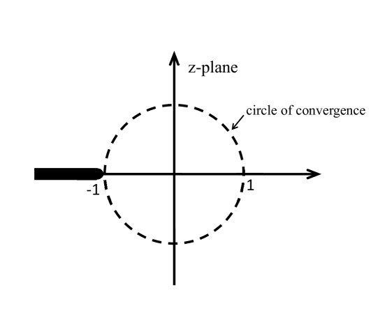
Figure 1: The analyticity area of the Fermi-Dirac integral $f_{\nu}\left(z\right)$ and the circle of convergence of the series in Eq. (2.5).

The analyticity area of the Fermi-Dirac integral $f_{\nu}\left(z\right)$ is shown in Fig. 1 [29, 30, 31]. From Fig. 1 we can see that the singularity in the $z-$plane of $f_{\nu}\left(z\right)$ begins with $-1$ to $-\infty$. Therefore, the radius of the circle of convergence of the series is $1$. However, we can also see from Fig. 1 that all points on the positive horizontal axis are analytical points. This implies that we can analytically continue $\sum_{n=1}^{\infty}\left(\pm 1\right)^{n+1}n^{l-D/2-1}z^{n}$ to whole positive horizontal axis; in other word, we can achieve an finite result of the sum of the series. Consequently, the result for the Fermi case is finite in the region $-1<z<\infty$. Then we have

$$\ln\Xi_{Fermi}=\sum_{l}B_{l}\frac{1}{\left(4\pi\right)^{l}}\lambda^{2l-D}f_{D/2+1-l}\left(z\right).$$ (2.6)

This result is finite for any non-negative $z$.

For the Bose case, the sum in Eq. (2.5) is converge and the summation can be done directly; the result for the Bose case has been obtained in Refs. [32]:

$$\ln\Xi_{Bose}=\sum_{l}B_{l}\frac{1}{\left(4\pi\right)^{l}}\lambda^{2l-D}g_{D/2+1-l}\left(z\right),$$ (2.7)

where $g_{\nu}\left(z\right)$ is the Bose-Einstein integral.

For convenience, in the following we express the grand potential of both Bose and Fermi gases as

$$\ln\Xi=\sum_{l=0,\frac{1}{2},1,\cdots}^{\infty}B_{l}\lambda^{2l-D}\frac{1}{\left(4\pi\right)^{l}}h_{D/2+1-l}\left(z\right),$$ (2.8)

where $h_{\nu}\left(z\right)=\frac{1}{\Gamma\left(\nu\right)}\int_{0}^{\infty}\frac{t^{\nu-1}}{z^{-1}e^{t}\mp 1}dt$ equals to Bose-Einstein integral $g_{\nu}\left(z\right)$ and Fermi-Dirac integral $f_{\nu}\left(z\right)$, respectively.

2.2 The expression of the equation of state and thermodynamic quantities

In this section, we give the expression of the equations of state and the corresponding thermodynamic quantities in quantum statistics.

According to Eq. (2.8), the equation of state is

$$\left\{\begin{array}[c]{c}\displaystyle\frac{pV}{kT}=\ln\Xi=\sum_{l=0,\frac{1}{2},1,\cdots}^{\infty}\frac{B_{l}}{\lambda^{D-2l}}\left(\frac{1}{4\pi}\right)^{l}h_{D/2+1-l}\left(z\right),\\ \displaystyle N=z\frac{\partial}{\partial z}\ln\Xi=\sum_{l=0,\frac{1}{2},1,\cdots}^{\infty}\frac{B_{l}}{\lambda^{D-2l}}\left(\frac{1}{4\pi}\right)^{l}h_{D/2-l}\left(z\right).\end{array}\right.$$ (2.9)

From Eq. (2.9), we can directly obtain various thermodynamic quantities: the internal energy

$$\frac{U}{kT}=-\beta\frac{\partial}{\partial\beta}\ln\Xi=\sum_{l=0,\frac{1}{2},1,\cdots}^{\infty}\frac{B_{l}}{\lambda^{D-2l}}\left(\frac{1}{4\pi}\right)^{l}\left(\frac{D}{2}-l\right)h_{D/2+1-l}\left(z\right),$$ (2.10)

the Helmholtz free energy

$$\frac{F}{kT} =-\ln\Xi+\frac{\mu}{kT}N$$

$$=\sum_{l=0,\frac{1}{2},1,\cdots}^{\infty}\frac{B_{l}}{\lambda^{D-2l}}\left(\frac{1}{4\pi}\right)^{l}\left[h_{D/2-l}\left(z\right)\ln z-h_{D/2+1-l}\left(z\right)\right],$$ (2.11)

the entropy

$$\frac{S}{k} =\frac{U-F}{kT}$$

$$=-N\ln z+\sum_{l=0,\frac{1}{2},1,\cdots}^{\infty}\frac{B_{l}}{\lambda^{D-2l}}\left(\frac{1}{4\pi}\right)^{l}\left[\left(\frac{D}{2}+1-l\right)h_{D/2+1-l}\left(z\right)\right],$$ (2.12)

and the specific heat

$$\frac{C_{V}}{k}=\frac{1}{k}\left(\frac{\partial U}{\partial T}\right)_{V}$$

$$=\sum_{l=0,\frac{1}{2},1,\cdots}^{\infty}\frac{B_{l}}{\lambda^{D-2l}}\left[\frac{D^{2}}{4}+\frac{D}{2}-\left(D+1\right)l+l^{2}\right]\left(\frac{1}{4\pi}\right)^{l}h_{D/2+1-l}\left(z\right)$$

$$\displaystyle-\frac{\left\{\sum_{l=0,\frac{1}{2},1,\cdots}^{\infty}\left(B_{l}/\lambda^{D-2l}\right)\left(\frac{D}{2}-l\right)\left[1/\left(4\pi\right)\right]^{l}h_{D/2-l}\left(z\right)\right\}^{2}}{\sum_{s=0,\frac{1}{2},1,\cdots}^{\infty}\left(B_{l}/\lambda^{D-2s}\right)\left[1/\left(4\pi\right)\right]^{s}h_{D/2-1-s}\left(z\right)},$$ (2.13)

where the relation

$$\frac{\partial z}{\partial T}=\displaystyle-\frac{z}{T}\frac{\sum_{l=0,\frac{1}{2},1,\cdots}^{\infty}\left(\frac{D}{2}-l\right)B_{l}\left[\lambda^{2}/\left(4\pi\right)\right]^{l}h_{D/2-l}\left(z\right)}{\sum_{s=0,\frac{1}{2},1,\cdots}^{\infty}B_{s}\left[\lambda^{2}/\left(4\pi\right)\right]^{s}h_{D/2-1-s}\left(z\right)}$$ (2.14)

is used when calculating the specific heat $C_{V}$.

3 Spectra and heat kernel coefficients in one-dimensional confined space with potentials

In this section, we calculate an approximate spectrum of a particle in one-dimensional confined space with an external potential. Moreover, we give the corresponding modified heat kernel coefficients. Some external potentials are considered.

3.1 Spectra: one dimension

The one-dimensional Schrödinger equation with the Dirichlet boundary condition is

$$\left\{\begin{array}[c]{l}\displaystyle\left(-\frac{\hbar^{2}}{2m}\frac{d^{2}}{dx^{2}}+V\left(x\right)\right)\psi\left(x\right)=E\psi\left(x\right),\\ \displaystyle\psi\left(0\right)=\psi\left(L\right)=0,\end{array}\right.$$ (3.1)

where $0<x<L$. According to Refs. [1, 2], we express the approximate spectrum as

$$E_{n}\simeq\frac{\pi^{2}\hbar^{2}}{2mL^{2}}\left[n^{2}+\int_{0}^{1}U\left(\xi\right)d\xi-\int_{0}^{1}U\left(\xi\right)\cos\left(2\pi n\xi\right)d\xi\right],\text{ }n=1,2,3,\cdots,$$ (3.2)

where $U\left(\xi\right)=\frac{2mL^{2}}{\pi^{2}\hbar^{2}}V\left(L\xi\right)$.

To give a more explicit expression to Eq. (3.2), we write the potential $U\left(\xi\right)$ as

$$U\left(\xi\right)=A\left(\xi\right)+S\left(\xi\right),$$ (3.3)

where the function $A\left(\xi\right)$ is an odd function with respect to the axis $\xi=\frac{1}{2}$ and $S\left(\xi\right)$ is an even one. The relations between $A\left(\xi\right)$, $S\left(\xi\right)$ and $U\left(\xi\right)$ are

$$\left\{\begin{array}[c]{c}A\left(\xi\right)=\frac{1}{2}\left[U\left(\xi\right)-U\left(1-\xi\right)\right]\\ S\left(\xi\right)=\frac{1}{2}\left[U\left(\xi\right)+U\left(1-\xi\right)\right]\end{array}\right..$$ (3.4)

Because of $\int_{0}^{1}A\left(\xi\right)d\xi=\int_{0}^{1}A\left(\xi\right)\cos\left(2\pi n\xi\right)d\xi=0$, we have

$$\int_{0}^{1}U\left(\xi\right)d\xi=\int_{0}^{1}S\left(\xi\right)d\xi,$$ (3.5)

and

$$\int_{0}^{1}U\left(\xi\right)\cos\left(2\pi n\xi\right)d\xi=\int_{0}^{1}S\left(\xi\right)\cos\left(2\pi n\xi\right)d\xi.$$ (3.6)

That is to say, only the even part $S\left(\xi\right)$ in the potential $U\left(\xi\right)$ contributes to the energy spectrum $E_{n}$ under the approximation, Eq. (3.2).

The even part $S\left(\xi\right)$ can always be expanded as

$$S\left(\xi\right)=\sum_{m=0}^{\infty}a_{m}\left(\xi-\frac{1}{2}\right)^{2m}.$$ (3.7)

Substituting Eq. (3.7) into Eqs. (3.5) and (3.6) and integrating term by term give

$$\int_{0}^{1}U\left(\xi\right)d\xi=\sum_{m=0}^{\infty}a_{m}\int_{0}^{1}\left(\xi-\frac{1}{2}\right)^{2m}d\xi=\sum_{m=0}^{\infty}\frac{a_{m}}{2^{2m}\left(2m+1\right)},$$ (3.8)

and

$$\int_{0}^{1}U\left(\xi\right)\cos\left(2\pi n\xi\right)d\xi$$

$$=\sum_{m=0}^{\infty}a_{m}\int_{0}^{1}\left(\xi-\frac{1}{2}\right)^{2m}\cos\left(2\pi n\xi\right)d\xi$$

$$=\sum_{m=0}^{\infty}a_{m}\left(-1\right)^{n+1}4^{-m}\frac{1}{2}\left[\mathcal{E}_{-2m}\left(-i\pi n\right)+\mathcal{E}_{-2m}\left(i\pi n\right)\right],$$ (3.9)

where $\mathcal{E}_{n}\left(z\right)=\int_{1}^{\infty}e^{-zt}t^{-n}dt$ is the exponential integral function. When $n\rightarrow\infty$,

$$\left(-1\right)^{n+1}4^{-m}\frac{1}{2}\left[\mathcal{E}_{-2m}\left(-i\pi n\right)+\mathcal{E}_{-2m}\left(i\pi n\right)\right]\simeq 2^{1-2m}\frac{m}{n^{2}\pi^{2}},$$ (3.10)

we then have

$$\int_{0}^{1}U\left(\xi\right)\cos\left(2\pi n\xi\right)d\xi\simeq\sum_{m=0}^{\infty}a_{m}\frac{m}{2^{2m-1}\pi^{2}n^{2}}.$$ (3.11)

Substituting Eqs. (3.8) and (3.11) into Eq. (3.2), we obtain a more explicit expression of energy spectrum to an arbitrary potential:

$$E_{n}\simeq\frac{\pi^{2}\hbar^{2}}{2mL^{2}}\left(n^{2}+\frac{\tilde{W}}{n^{2}}+\tilde{U}\right),\text{ \ \ }n=1,2,3,\cdots,$$ (3.12)

where

$$\tilde{U}=\sum_{m=0}^{\infty}\frac{a_{m}}{2^{2m}\left(2m+1\right)}$$ (3.13)

and

$$\tilde{W}=-\frac{1}{\pi^{2}}\sum_{m=1}^{\infty}a_{m}\frac{m}{2^{2m-1}}.$$ (3.14)

3.2 Heat kernel coefficients: one dimension

With the energy spectrum Eq. (3.12), we can directly express the global heat kernel as

$$K\left(t\right)\simeq\exp\left(-t\frac{\pi^{2}}{L^{2}}\tilde{U}\right)\sum_{n=1}^{\infty}\exp\left[-t\frac{\pi^{2}}{L^{2}}\left(n^{2}+\frac{\tilde{W}}{n^{2}}\right)\right].$$ (3.15)

Using the Euler-Maclaurin formula [33]

$$\sum_{n=a}^{b}f\left(n\right) =\int_{a}^{b}f\left(n\right)dn+\frac{1}{2}\left[f\left(a\right)+f\left(b\right)\right]$$

$$+\sum_{k=1}^{m}\frac{\mathcal{B}_{2k}}{\left(2k\right)!}\left[f^{\left(2k-1\right)}\left(b\right)-f^{\left(2k-1\right)}\left(a\right)\right]$$

$$+\frac{1}{\left(2m+1\right)!}\int_{a}^{b}\mathcal{B}_{2m+1}\left(x-\left\lfloor x\right\rfloor\right)f^{\left(2m+1\right)}\left(x\right)dx,$$ (3.16)

where $\mathcal{B}_{2k}$ is Bernoulli number, $\mathcal{B}_{2k}\left(x\right)$ is Bernoulli polynomial, and $\left\lfloor x\right\rfloor$ is the maximum integer which is no more than $x$, taking $m=1$ and omitting the remainder term, we obtain

$$K\left(t\right) \simeq\frac{1}{\sqrt{4\pi t}}\exp\left(-t\frac{\pi^{2}}{L^{2}}\tilde{U}\right)\times$$

$$\left\{\frac{L}{2}\left\{\exp\left(-2\frac{\pi^{2}}{L^{2}}\sqrt{\tilde{W}}t\right)\operatorname{erfc}\left[\frac{\pi}{L}\left(1-\sqrt{\tilde{W}}\right)\sqrt{t}\right]\right.\right.$$

$$\left.+\exp\left(2\frac{\pi^{2}}{L^{2}}\sqrt{\tilde{W}}t\right)\operatorname{erfc}\left[\frac{\pi}{L}\left(1+\sqrt{\tilde{W}}\right)\sqrt{t}\right]\right\}$$

$$\left.+\frac{\sqrt{4\pi t}}{6}\left[3+t\frac{\pi^{2}}{L^{2}}\left(1-\tilde{W}\right)\right]\exp\left[-t\frac{\pi^{2}}{L^{2}}\left(1+\tilde{W}\right)\right]\right\},$$ (3.17)

where $\operatorname{erfc}\left(z\right)$ is the complementary error function [34].

Expanding the global heat kernel Eq. (3.17) as the form of Eq. (1.2) gives the heat kernel coefficients:

$$B_{0}=L,$$ (3.18)

$$B_{1/2}=\pi^{1/2}\left(1-2\tilde{W}^{1/2}\right),$$ (3.19)

$$B_{1}=-\frac{\pi^{2}}{L}\tilde{U},$$ (3.20)

$$B_{3/2}=-\frac{\pi^{5/2}}{3L^{2}}\left[2+3\tilde{U}+6\left(1-\tilde{U}\right)\tilde{W}^{1/2}+4\tilde{W}-2\tilde{W}^{3/2}\right],$$ (3.21)

$$B_{2}=\frac{\pi^{4}}{2L^{3}}\left(\tilde{U}^{2}+4\tilde{W}\right),$$ (3.22)

$$B_{5/2} =\frac{\pi^{9/2}}{30L^{4}}\left[5+20\tilde{U}+15\tilde{U}^{2}+10\left(1+6\tilde{U}-30\tilde{U}^{2}\right)\tilde{W}^{1/2}\right.$$

$$\left.+10\left(3+4\tilde{U}\right)\tilde{W}-20\left(3+\tilde{U}\right)\tilde{W}^{3/2}+25\tilde{W}^{2}-6\tilde{W}^{5/2}\right],$$ (3.23)

$$B_{3}=-\frac{\pi^{6}}{6L^{5}}\left(\tilde{U}^{3}+12\tilde{U}\tilde{W}\right),$$ (3.24)

$$B_{7/2} =-\frac{\pi^{13/2}}{210L^{6}}\left[35\left(\tilde{U}+2\tilde{U}^{2}+\tilde{U}^{3}\right)\right.$$

$$\left.+14\left(1+5\tilde{U}+15\tilde{U}^{2}-5\tilde{U}^{3}\right)\tilde{W}^{1/2}+70\left(1+3\tilde{U}+2\tilde{U}^{2}\right)\tilde{W}\right.$$

$$\left.+70\left(3-6\tilde{U}-\tilde{U}^{2}\right)\tilde{W}^{3/2}+35\left(4+5\tilde{U}\right)\tilde{W}^{2}\right.$$

$$\left.-14\left(5+3\tilde{U}\right)\tilde{W}^{5/2}+70\tilde{W}^{3}-10\tilde{W}^{7/2}\right],$$ (3.25)

$$B_{4}=\frac{\pi^{8}}{24L^{7}}(\tilde{U}^{4}+24\tilde{U}^{2}\tilde{W}+16\tilde{W}^{2}),$$ (3.26)

$$B_{9/2} =\frac{\pi^{17/2}}{7560L^{8}}\left[105\left(-1+6\tilde{U}^{2}+8\tilde{U}^{3}+3\tilde{U}^{4}\right)\right.$$

$$\left.18\left(5+28\tilde{U}+70\tilde{U}^{2}+140\tilde{U}^{3}-35\tilde{U}^{4}\right)\tilde{W}^{1/2}\right.$$

$$\left.420\left(1+6\tilde{U}+9\tilde{U}^{2}+4\tilde{U}^{3}\right)\tilde{W}\right.$$

$$\left.+840\left(1+9\tilde{U}-9\tilde{U}^{2}-\tilde{U}^{3}\right)\tilde{W}^{3/2}\right.$$

$$\left.+630\left(3+8\tilde{U}+5\tilde{U}^{2}\right)\tilde{W}^{2}-252\left(15+10\tilde{U}+3\tilde{U}^{2}\right)\tilde{W}^{5/2}\right.$$

$$\left.+420(5+6\tilde{U})\tilde{W}^{3}-72(7+5\tilde{U})\tilde{W}^{7/2}+735\tilde{W}^{4}-70\tilde{W}^{9/2}\right],$$ (3.27)

$$B_{5}=-\frac{\pi^{10}}{120L^{9}}\left(\tilde{U}^{5}+40\tilde{U}^{3}\tilde{W}+80\tilde{U}\tilde{W}^{2}\right),$$ (3.28)

and so on. We find that the modification of the heat kernel coefficients caused by the term $\int_{0}^{1}U\left(\xi\right)d\xi$ and $\int_{0}^{1}U\left(\xi\right)\cos\left(2\pi n\xi\right)d\xi$ begins at $B_{1}$ and $B_{3/2}$, respectively.

3.3 Various external potentials: examples

In the following, as examples, we consider various external potentials in confined space.

(1) For the external potential

$$U\left(\xi\right)=\frac{U_{0}}{\sqrt{2\pi}\sigma}\exp\left[-\frac{1}{2\sigma^{2}}\left(\xi-\frac{1}{2}\right)^{2}\right],$$

the coefficient in Eqs. (3.13) and (3.14) reads

$$a_{m}=U_{0}\frac{2^{-1/2-m}\sigma^{-1-2m}}{\sqrt{\pi}m!}.$$ (3.29)

By Eqs. (3.13), (3.14), and (3.7), we achieve

$$\tilde{U}=U_{0}\operatorname{erfi}\left(\frac{1}{2\sqrt{2}\sigma}\right)\text{ and\ }\tilde{W}=-U_{0}\frac{e^{1/\left(8\sigma^{2}\right)}}{4\sqrt{2}\pi^{5/2}\sigma^{3}},$$ (3.30)

where $\operatorname{erfi}\left(z\right)$ is the imaginary error function [34].

(2) For the external potential

$$U\left(\xi\right)=U_{0}\left\{\left[\left(\xi-\frac{1}{2}\right)^{2}-\frac{1}{8}\alpha^{2}\right]^{2}-\frac{1}{64}\alpha^{4}\right\},\text{ \ \ }\left(0<\alpha<1\right),$$ (3.31)

we have

$$a_{0}=0,\text{ \ \ }a_{1}=-\frac{\alpha^{2}}{4}U_{0},\text{ \ \ }a_{2}=U_{0},\text{ \ \ }a_{m}=0\text{ \ \ }\left(m\geq 3\right),$$ (3.32)

and then achieve

$$\tilde{U}=U_{0}\left(\frac{1}{80}-\frac{\alpha^{2}}{48}\right)\text{ and\ }\tilde{W}=\frac{U_{0}}{8\pi^{2}}\left(\alpha^{2}-2\right).$$ (3.33)

(3) For the external potential

$$U\left(\xi\right)=U_{0}\alpha^{2}e^{\alpha^{2}(\xi-1/2)^{2}}\left(\xi-\frac{1}{2}\right)^{2}\left[1+\alpha^{2}\left(\xi-\frac{1}{2}\right)^{2}\right],$$ (3.34)

we have

$$a_{m}=\frac{m^{2}}{m!}\alpha^{2m},\text{ \ \ }m=0,1,2,\cdots,$$ (3.35)

and then achieve

$$\tilde{U}=\frac{1}{8}\left[2\sqrt{\pi}\operatorname{erfi}\left(\frac{1}{2}\right)-e^{1/4}\right]\text{ and\ }\tilde{W}=-\frac{29e^{1/4}}{32\pi^{2}}.$$ (3.36)

4 Spectra and heat kernel coefficients in $D\left(\geq 2\right)$-dimensional confined space

In this section, the ideal gas in the $D$-dimensional $\left(D\geq 2\right)$ confined space is discussed. We calculate the modification of external potentials to global heat kernel in confined space. The method given by Ref. [3] is used to acquire the approximate energy spectrum. Specifically, we provide the modified heat kernel coefficients in two-dimensional confined space and three-dimensional confined ball. Some external potentials are considered.

In fact, the heat kernel technique is a high frequency asymptotics method. The method provided by Ref. [3] achieves the asymptotics of eigenvalues in confined space. The key step in Ref. [3] is to take a high frequency approximation to the matrix element. Such an approximation reveals what essentially one has done in Weyl and Kac’s famous high frequency asymptotics for the heat kernel, although it is just equivalent to substituting an external potential with its meanvalue in the confined space.

4.1 Spectra and heat kernel coefficients: $D\left(\geq 2\right)$ dimensions

According to Ref. [3], the approximate eigenvalues of the equation

$$\left\{\begin{array}[c]{l}\displaystyle\left(-\frac{\hbar^{2}}{2m}\Delta+U\right)\psi=E\psi,\text{ \ \ in \ \ }\Omega\\ \displaystyle\psi=0,\text{ \ \ on \ \ }\partial\Omega\end{array}\right.$$ (4.1)

are

$$E_{s}\simeq E_{s}^{\left(0\right)}+\tilde{U},$$ (4.2)

where

$$\tilde{U}=\frac{1}{V}\int_{\Omega}U\left(x\right)dV$$ (4.3)

and $\Omega$ represents the region of space.

Obviously, the global heat kernel in $D$-dimensional $\left(D\geq 2\right)$ confined space is

$$K\left(t\right) =\sum_{s}\exp\left(-t\frac{2mE_{s}}{\hbar^{2}}\right)$$

$$=\left(4\pi t\right)^{-D/2}\sum_{l=0,\frac{1}{2},1,\cdots}^{\infty}B_{l}t^{l},$$ (4.4)

where $B_{l}$ is the heat kernel coefficient of the operator $-\Delta+\frac{2m}{\hbar^{2}}V$. Substituting Eq. (4.2) into Eq. (4.4), we have

$$K\left(t\right) \simeq\sum_{s}\exp\left[-t\frac{2m}{\hbar^{2}}\left(E_{s}^{\left(0\right)}+\tilde{U}\right)\right]$$

$$=\exp\left(-t\frac{2m\tilde{U}}{\hbar^{2}}\right)\sum_{s}\exp\left(-\frac{2mE_{s}^{\left(0\right)}}{\hbar^{2}}t\right)$$

$$=\exp\left(-t\tilde{U}\right)K^{\left(0\right)}\left(t\right),$$ (4.5)

where $K^{\left(0\right)}\left(t\right)=\left(4\pi t\right)^{-D/2}\sum_{\kappa=0,\frac{1}{2},1,\cdots}^{\infty}B_{\kappa}^{\left(0\right)}t^{\kappa}$ is the global heat kernel of $-\Delta$ in the region $\Omega$. Substituting $\exp\left(-t\frac{2m\tilde{U}}{\hbar^{2}}\right)=\sum_{\sigma=0}^{\infty}\frac{\left(-1\right)^{\sigma}}{\sigma!}\left(\frac{2m\tilde{U}}{\hbar^{2}}\right)^{\sigma}t^{\sigma}$ into Eq. (4.5), we obtain the modified heat kernel coefficient

$$B_{l}=\sum_{s=0}^{\left\lfloor l\right\rfloor}\frac{\left(-1\right)^{s}}{s!}\left(\frac{2m\tilde{U}}{\hbar^{2}}\right)^{s}B_{l-s}^{\left(0\right)},\text{\ }l=0,\frac{1}{2},1,\cdots,$$ (4.6)

where $\left\lfloor l\right\rfloor$ is the maximum integer no more than $l$. The first three coefficients are

$$B_{0}=B_{0}^{\left(0\right)},\text{ \ \ }B_{1/2}=B_{1/2}^{\left(0\right)},\text{ \ \ }B_{1}=B_{1}^{\left(0\right)}-\frac{2m\tilde{U}}{\hbar^{2}}B_{0}^{\left(0\right)}.$$ (4.7)

4.2 Heat kernel coefficients in two-dimensional confined space

The global heat kernel of $-\Delta$ in two-dimensional confined space without holes, indicated by Kac [8], has the asymptotic expression

$$K^{\left(0\right)}\left(t\right)\simeq\frac{A}{4\pi t}-\frac{L}{2\sqrt{\pi t}}+\frac{1}{6},$$ (4.8)

where $A$ is the area and $L$ is the perimeter of the region.

When the external potential exists, according to Eq. (4.6), the modified heat kernel coefficients are

$$B_{0}=A,\text{ }B_{1/2}=-2\sqrt{\pi}L,\text{ }B_{1}=\frac{2\pi}{3}-\frac{2m\tilde{U}}{\hbar^{2}}A,$$ (4.9)

and the asymptotic expression of the corresponding modified global heat kernel in two-dimensional confined space is

$$K\left(t\right)\simeq\frac{A}{4\pi t}-\frac{L}{2\sqrt{\pi t}}+\left(\frac{1}{6}-\frac{A}{4\pi}\frac{2m\tilde{U}}{\hbar^{2}}\right).$$ (4.10)

4.3 Heat kernel coefficients in a three-dimensional ball

The global heat kernel of $-\Delta$ in a three-dimensional ball has the asymptotic expression [35]

$$K^{\left(0\right)}\left(t\right)\simeq\frac{1}{\left(4\pi t\right)^{3/2}}\left(\frac{4}{3}\pi R^{3}-2\pi^{3/2}R^{2}\sqrt{t}+\frac{8}{3}\pi Rt\right),$$ (4.11)

where $R$ is the radius of the ball.

When there is an external potential in the ball, using Eq. (4.6), we obtain the modified heat kernel coefficients

$$B_{0}=\frac{4}{3}\pi R^{3},\text{ \ \ }B_{1/2}=-2\pi^{3/2}R^{2},\text{ \ \ }B_{1}=\frac{8}{3}\pi R\left(1-\frac{R^{2}}{2}\frac{2m\tilde{U}}{\hbar^{2}}\right).$$ (4.12)

The corresponding asymptotic expression of the modified global heat kernel in the three-dimensional ball is

$$K\left(t\right)\simeq\frac{1}{\left(4\pi t\right)^{3/2}}\left[\frac{4}{3}\pi R^{3}-2\pi^{3/2}R^{2}\sqrt{t}+\frac{8}{3}\pi R\left(1-\frac{R^{2}}{2}\frac{2m\tilde{U}}{\hbar^{2}}\right)t\right].$$ (4.13)

4.4 Various spherically symmetric external potentials in $D\left(\geq 2\right)$-dimensional balls: examples

In this section, as examples, we consider some spherically symmetric external potentials $U\left(x\right)$. According to the above analysis, the modification of the heat kernel coefficients caused by the external potential $U\left(x\right)$ is approximately determined by the quantity $\tilde{U}$.

The effect of a spherically symmetric potential to the energy level in a $D$-dimensional $\left(D\geq 2\right)$ ball is

$$\tilde{U} =\frac{1}{V_{ball}}\int_{\Omega}U\left(r\right)dV$$

$$=\frac{1}{V_{ball}}\int_{0}^{R}U\left(r\right)r^{D-1}dr\left(\int_{0}^{2\pi}d\varphi\right)\left(\prod\limits_{n=1}^{D-2}\int_{0}^{\pi}\sin^{n}\theta d\theta\right)$$

$$=\frac{2}{R^{D}}\frac{\Gamma\left(1+\frac{D}{2}\right)}{\Gamma\left(\frac{D}{2}\right)}\int_{0}^{R}U\left(r\right)r^{D-1}dr,$$ (4.14)

where $R$ is the radius of balls, then we have

$$\tilde{U}=\frac{D}{R^{D}}\int_{0}^{R}U\left(r\right)r^{D-1}dr.$$ (4.15)

(1) For the external potential

$$U\left(r\right)=-\frac{U_{0}R^{2}}{\sqrt{2\pi}a^{2}}\exp\left(-\frac{r^{2}}{2a^{2}}\right),$$ (4.16)

from Eq. (4.14), we achieve

$$\tilde{U}=-U_{0}\frac{D}{\sqrt{\pi}}2^{\left(D-3\right)/2}\left(\frac{a}{R}\right)^{D-2}\left[\Gamma\left(\frac{D}{2}\right)-\Gamma\left(\frac{D}{2},\frac{R^{2}}{2a^{2}}\right)\right].$$ (4.17)

(2) For the external potential

$$U=-U_{0}\frac{R^{s}}{r^{s}},\text{ \ \ }s\leq D-1,$$ (4.18)

we achieve

$$\tilde{U}=-U_{0}\frac{D}{D-s}.$$ (4.19)

(3) For the external potential

$$U\left(r\right)=-U_{0}\frac{\alpha\left(\alpha-1\right)}{\cosh^{2}\left(r/a\right)},$$ (4.20)

we achieve

$$\tilde{U}=-\alpha\left(\alpha-1\right)U_{0}\frac{R^{2}}{a^{2}}\frac{D}{R^{D}}\int_{0}^{R}r^{D-1}\operatorname{sech}^{2}\left(\frac{r}{a}\right)dr.$$ (4.21)

When $D=2$,

$$\tilde{U}=-2\alpha\left(\alpha-1\right)U_{0}\left[\ln\left(\operatorname{sech}\frac{R}{a}\right)+\frac{R}{a}\tanh\frac{R}{a}\right];$$ (4.22)

when $D=3$,

$$\tilde{U} =-\alpha\left(\alpha-1\right)U_{0}\left[\frac{\pi^{2}}{4}\frac{a}{R}-3\frac{R}{a}-6\ln\left(1+e^{-2R/a}\right)\right.$$

$$\left.-3\frac{a}{R}f_{2}\left(e^{-2R/a}\right)+3\frac{R}{a}\tanh\frac{R}{a}\right].$$ (4.23)

5 The effect of boundaries and potentials to ideal quantum gases

In this section, we calculate the thermodynamic properties of ideal gases in confined space with an external potential. First, we discuss the properties of ideal gases under the condition of weak degeneration. We give the virial expansion of the equation of state. Second, we discuss the properties of ideal gases under the condition of complete degeneration. We obtain the asymptotic expression of the specific heat at low temperatures and high densities.

5.1 Weak degenerate ideal quantum gases in confined space with potentials

In this section, we consider weak degenerate ideal quantum gases. The virial expression of the equation of state is given, which is modified by the boundary and the potential.

According to the equation of state Eq. (2.9), we obtain

$$\frac{pV}{NkT}=\frac{\sum_{l=0,\frac{1}{2},1,\cdots}^{\infty}B_{l}\left[\lambda^{2}/\left(4\pi\right)\right]^{l}h_{D/2+1-l}\left(z\right)}{\sum_{s=0,\frac{1}{2},1,\cdots}^{\infty}B_{s}\left[\lambda^{2}/\left(4\pi\right)\right]^{s}h_{D/2-s}\left(z\right)},$$ (5.1)

$$\frac{n\lambda^{D}}{g}=\sum_{l=0,\frac{1}{2},1,\cdots}^{\infty}\frac{B_{l}}{B_{0}}\left(\frac{\lambda^{2}}{4\pi}\right)^{l}h_{D/2-l}\left(z\right),$$ (5.2)

where $n=N/V$ is the number density and $g$ is a weight factor arising form the internal structure of the particle; noting that $B_{0}=V$, the volume. Truncating Eqs. (5.1) and (5.2) up to $B_{1}$ and then expanding them with respect to $z$, we obtain

$$\frac{pV}{NkT} =\frac{B_{0}h_{D/2+1}\left(z\right)+\frac{\lambda}{\sqrt{4\pi}}B_{1/2}h_{D/2+1/2}\left(z\right)+\frac{\lambda^{2}}{4\pi}B_{1}h_{D/2}\left(z\right)}{B_{0}h_{D/2}\left(z\right)+\frac{\lambda}{\sqrt{4\pi}}B_{1/2}h_{D/2-1/2}+\frac{\lambda^{2}}{4\pi}B_{1}h_{D/2-1}\left(z\right)}$$

$$=1\mp\frac{2^{-\mathcal{D}/2}\left(2\pi B_{0}+\sqrt{2\pi}\lambda B_{1/2}+\lambda^{2}B_{1}\right)}{4\pi B_{0}+2\sqrt{\pi}\lambda B_{1/2}+\lambda^{2}B_{1}}z+\cdots,$$ (5.3)

and

$$\frac{n\lambda^{D}}{g}=h_{D/2}\left(z\right)+\frac{\lambda}{\sqrt{4\pi}}\frac{B_{1/2}}{B_{0}}h_{D/2-1/2}\left(z\right)+\frac{\lambda^{2}}{4\pi}\frac{B_{1}}{B_{0}}h_{D/2-1}\left(z\right)+\cdots.$$ (5.4)

Inverting the series in Eq. (5.4), we obtain an expression for $z$ in powers of $n\lambda^{D}/g$,

$$z =\frac{1}{1+\lambda B_{1/2}/\left(2\sqrt{\pi}B_{0}\right)+\lambda^{2}B_{1}/\left(4\pi B_{0}\right)}\frac{n\lambda^{D}}{g}$$

$$\mp\frac{2^{5-D/2}\pi^{2}B_{0}^{2}\left(2\pi B_{0}+\sqrt{2\pi}\lambda B_{1/2}+\lambda^{2}B_{1}\right)}{\left(4\pi B_{0}+2\sqrt{\pi}\lambda B_{1/2}+\lambda^{2}B_{1}\right)^{3}}\left(\frac{n\lambda^{D}}{g}\right)^{2}+\cdots,$$ (5.5)

Substituting Eq. (5.5) into Eq. (5.3), the virial expansion is

$$\frac{pV}{NkT}=1\mp\frac{n\lambda^{D}}{g}\left[\frac{1}{2^{D/2+1}}-\frac{\sqrt{2}-1}{2^{\left(D+3\right)/2}}\frac{\lambda B_{1/2}}{\sqrt{\pi}B_{0}}-\frac{2-\sqrt{2}}{2^{\left(D+7\right)/2}}\frac{\lambda^{3}B_{1/2}B_{1}}{\pi^{3/2}B_{0}^{2}}\right]+\cdots.$$ (5.6)

The other thermodynamic quantities are the internal energy

$$\frac{U}{NkT} =\left(\frac{D}{2}-\frac{\lambda B_{1/2}}{4\sqrt{\pi}B_{0}}-\frac{\lambda^{2}B_{1}}{4\pi B_{0}}+\frac{3\lambda^{3}B_{1/2}B_{1}}{16\pi^{3/2}B_{0}^{2}}\right)$$

$$\mp\frac{n\lambda^{D}}{g}\left[\frac{1}{2^{D/2+2}}-\frac{\sqrt{2}-1}{2^{\left(D+5\right)/2}}\left(D+1\right)\frac{\lambda B_{1/2}}{\sqrt{\pi}B_{0}}\right.$$ (5.7)

$$\left.-\frac{2-\sqrt{2}}{2^{\left(D+9\right)/2}}\left(D+3\right)\frac{\lambda^{3}B_{1/2}B_{1}}{\pi^{3/2}B_{0}^{2}}\right]+\cdots,$$ (5.8)

the Helmholtz free energy

$$\frac{F}{NkT} =\left[\ln\left(\frac{n\lambda^{D}}{g}\right)-1-\frac{\lambda B_{1/2}}{2\sqrt{\pi}B_{0}}-\frac{\lambda^{2}B_{1}}{4\pi B_{0}}+\frac{\lambda^{3}B_{1/2}B_{1}}{8\pi^{3/2}B_{0}^{2}}\right]$$

$$\mp\frac{n\lambda^{D}}{g}\left[\frac{1}{2^{D/2+1}}-\frac{\sqrt{2}-1}{2^{\left(D+3\right)/2}}\frac{\lambda B_{1/2}}{\sqrt{\pi}B_{0}}\right.$$

$$\left.-\frac{\sqrt{2}-1}{2^{D/2+3}}\frac{\lambda^{3}B_{1/2}B_{1}}{\pi^{3/2}B_{0}^{2}}\right]+\cdots,$$ (5.9)

the entropy

$$\frac{S}{Nk} =\left[1+\frac{D}{2}+\frac{\lambda B_{1/2}}{4\sqrt{\pi}B_{0}}+\frac{\lambda^{3}B_{1/2}B_{1}}{16\pi^{3/2}B_{0}^{2}}-\ln\left(\frac{n\lambda^{D}}{g}\right)\right]$$

$$\mp\frac{n\lambda^{D}}{g}\left[\frac{1}{2^{D/2+2}}\left(D-2\right)-\frac{\sqrt{2}-1}{2^{\left(D+5\right)/2}}\left(D-1\right)\frac{\lambda B_{1/2}}{\sqrt{\pi}B_{0}}\right.$$

$$\left.-\frac{\sqrt{2}-1}{2^{D/2+4}}\left(D+1\right)\frac{\lambda^{3}B_{1/2}B_{1}}{\pi^{3/2}B_{0}{}^{2}}\right]+\cdots,$$ (5.10)

and the specific heat

$$\frac{C_{V}}{Nk} =\left(\frac{D}{2}-\frac{\lambda B_{1/2}}{8\sqrt{\pi}B_{0}}-\frac{3\lambda^{3}B_{1/2}B_{1}}{32\pi^{3/2}B_{0}{}^{2}}\right)$$

$$\pm\frac{n\lambda^{D}}{g}\left[\frac{1}{2^{D/2+3}}\left(D^{2}-2D\right)-\frac{\sqrt{2}-1}{2^{\left(D+7\right)/2}}\left(D^{2}-1\right)\frac{\lambda B_{1/2}}{\sqrt{\pi}B_{0}}\right.$$

$$\left.-\frac{\sqrt{2}-1}{2^{D/2+5}}\left(D^{2}+4D+3\right)\frac{\lambda^{3}B_{1/2}B_{1}}{\pi^{3/2}B_{0}^{2}}\right]+\cdots.$$ (5.11)

5.2 Completely degenerate ideal quantum gases in confined space with potentials

In this section, we discuss the property of completely degenerate ideal gases. We consider ideal Bose gases in two dimensions and ideal Fermi gases in two and three dimensions. We obtain asymptotic expressions of the chemical potential and specific heat at low temperatures and high densities for Bose and Fermi gases, which show the influence of the boundary and potential.

5.2.1 Ideal Fermi gases in two-dimensional confined space with potentials

From Eqs. (2.13) and (2.9), for a Fermi gas, when $D=2$, the specific heat and the number density are

$$\frac{C_{V}}{Nk}$$

$$=\frac{\sum_{l=0,\frac{1}{2},1,\cdots}^{\infty}B_{l}\left(l^{2}-3l+2\right)\left[\lambda^{2}/\left(4\pi\right)\right]^{l}f_{2-l}\left(z\right)}{\sum_{s=0,\frac{1}{2},1,\cdots}^{\infty}B_{s}\left[\lambda^{2}/\left(4\pi\right)\right]^{s}f_{1-s}\left(z\right)}$$

$$-\frac{\left\{\sum_{l=0,\frac{1}{2},1,\cdots}^{\infty}B_{l}\left(1-l\right)\left[\lambda^{2}/\left(4\pi\right)\right]^{l}f_{1-l}\left(z\right)\right\}^{2}}{\sum_{s=0,\frac{1}{2},1,\cdots}^{\infty}\sum_{j=0,\frac{1}{2},1,\cdots}^{\infty}B_{s}B_{j}\left[\lambda^{2}/\left(4\pi\right)\right]^{s+j}f_{1-s}\left(z\right)f_{-j}\left(z\right)},$$ (5.12)

and

$$\frac{n\lambda^{2}}{g}=\sum_{l=0,\frac{1}{2},1,\cdots}^{\infty}\frac{B_{l}}{B_{0}}\left(\frac{\lambda^{2}}{4\pi}\right)^{l}f_{1-l}\left(z\right).$$ (5.13)

Truncating Eqs. (5.12) and (5.13) up to $B_{1}$ and then using [36]

$$f_{\nu}\left(z\right) =\frac{\left(\ln z\right)^{\nu}}{\Gamma\left(\nu+1\right)}\left[1+\nu\left(\nu-1\right)\frac{\pi^{2}}{6}\left(\ln z\right)^{-2}\right.$$

$$\left.+\nu\left(\nu-1\right)\left(\nu-2\right)\left(\nu-3\right)\frac{7\pi^{4}}{360}\left(\ln z\right)^{-4}+\cdots\right],$$ (5.14)

we obtain $C_{V}/\left(Nk\right)$ and $n\lambda^{2}/g$ in powers of $kT/\mu$,

$$\frac{C_{V}}{Nk} =\frac{\pi^{2}}{3}\frac{kT}{\mu}-\frac{\pi\lambda B_{1/2}}{6B_{0}}\left(\frac{kT}{\mu}\right)^{3/2}+\left(\frac{\lambda^{2}B_{1/2}^{2}}{6B_{0}^{2}}-\frac{\pi\lambda^{2}B_{1}}{12B_{0}}\right)\left(\frac{kT}{\mu}\right)^{2}$$

$$-\left(\frac{\lambda^{3}B_{1/2}^{3}}{6\pi B_{0}^{3}}-\frac{\lambda^{3}B_{1/2}B_{1}}{8B_{0}^{2}}\right)\left(\frac{kT}{\mu}\right)^{5/2}+\cdots,$$ (5.15)

and

$$\frac{n\lambda^{2}}{g} =\frac{\mu}{kT}\left[1+\frac{\lambda^{2}B_{1}}{4\pi B_{0}}\frac{kT}{\mu}+\frac{\lambda B_{1/2}}{\pi B_{0}}\left(\frac{kT}{\mu}\right)^{3/2}\right.$$

$$\left.-\frac{\pi\lambda B_{1/2}}{24B_{0}}\left(\frac{kT}{\mu}\right)^{5/2}-\frac{7\pi^{3}\lambda B_{1/2}}{384B_{0}}\left(\frac{kT}{\mu}\right)^{9/2}+\cdots\right].$$ (5.16)

From Eq. (5.16), we have

$$\mu =\varepsilon_{F}\left[1-\frac{\lambda B_{1/2}}{\pi B_{0}}\left(\frac{kT}{\mu}\right)^{1/2}+\left(\frac{\lambda^{2}B_{1/2}^{2}}{\pi^{2}B_{0}^{2}}-\frac{\lambda^{2}B_{1}}{4\pi B_{0}}\right)\frac{kT}{\mu}\right.$$

$$\left.-\left(\frac{\lambda^{3}B_{1/2}^{3}}{\pi^{3}B_{0}^{3}}-\frac{\lambda^{3}B_{1/2}B_{1}}{2\pi^{2}B_{0}^{2}}\right)\left(\frac{kT}{\mu}\right)^{3/2}\right.$$

$$\left.+\left(\frac{\lambda^{4}B_{1/2}^{4}}{\pi^{4}B_{0}^{4}}-\frac{3\lambda^{4}B_{1/2}^{2}B_{1}}{4\pi^{3}B_{0}^{3}}+\frac{\lambda^{4}B_{1}^{2}}{16\pi^{2}B_{0}^{2}}\right)\left(\frac{kT}{\mu}\right)^{2}+\cdots\right],$$ (5.17)

where $\varepsilon_{F}=nh^{2}/\left(2\pi gm\right)$ is the two-dimensional Fermi energy. Inverting the series in Eq. (5.17) to obtain an expansion for $\mu$ in powers of $kT/\varepsilon_{F}$,

$$\mu =\varepsilon_{F}\left[1-\frac{\lambda B_{1/2}}{\pi B_{0}}\left(\frac{kT}{\varepsilon_{F}}\right)^{1/2}+\left(\frac{\lambda^{2}B_{1/2}^{2}}{2\pi^{2}B_{0}^{2}}-\frac{\lambda^{2}B_{1}}{4\pi B_{0}}\right)\frac{kT}{\varepsilon_{F}}\right.$$

$$\left.-\left(\frac{\lambda^{3}B_{1/2}^{3}}{8\pi^{3}B_{0}^{3}}-\frac{\lambda^{3}B_{1/2}B_{1}}{8\pi^{2}B_{0}^{2}}\right)\left(\frac{kT}{\varepsilon_{F}}\right)^{3/2}\right.$$

$$\left.+\left(\frac{129\lambda^{5}B_{1/2}^{5}}{128\pi^{5}B_{0}^{5}}-\frac{65\lambda^{5}B_{1/2}^{3}B_{1}}{64\pi^{4}B_{0}^{4}}+\frac{25\lambda^{5}B_{1/2}B_{1}^{2}}{128\pi^{3}B_{0}^{3}}\right)\left(\frac{kT}{\varepsilon_{F}}\right)^{5/2}\right.$$

$$\left.+\left(\frac{2\lambda^{6}B_{1/2}^{6}}{\pi^{6}B_{0}^{6}}-\frac{7\lambda^{6}B_{1/2}^{4}B_{1}}{4\pi^{5}B_{0}^{5}}+\frac{3\lambda^{6}B_{1/2}^{2}B_{1}^{2}}{16\pi^{4}B_{0}^{4}}+\frac{\lambda^{6}B_{1}^{3}}{64\pi^{3}B_{0}^{3}}\right)\left(\frac{kT}{\varepsilon_{F}}\right)^{3}+\cdots\right],$$ (5.18)

and then substituting Eq. (5.18) into Eq. (5.15), we obtain the asymptotic expression of the specific heat at low temperatures and high densities

$$\frac{C_{V}}{Nk} =\frac{\pi^{2}}{3}\frac{kT}{\varepsilon_{F}}+\frac{\pi\lambda B_{1/2}}{6B_{0}}\left(\frac{kT}{\varepsilon_{F}}\right)^{3/2}+\frac{\lambda^{2}B_{1/2}^{2}}{12B_{0}^{2}}\left(\frac{kT}{\varepsilon_{F}}\right)^{2}$$

$$+\left(\frac{3\lambda^{3}B_{1/2}^{3}}{16\pi B_{0}^{3}}-\frac{5\lambda^{3}B_{1/2}B_{1}}{48B_{0}^{2}}\right)\left(\frac{kT}{\varepsilon_{F}}\right)^{5/2}$$

$$+\left(\frac{\lambda^{4}B_{1/2}^{4}}{4\pi^{2}B_{0}^{4}}-\frac{\lambda^{4}B_{1/2}^{2}B_{1}}{8\pi B_{0}^{3}}-\frac{\lambda^{4}B_{1}^{2}}{48B_{0}^{2}}\right)\left(\frac{kT}{\varepsilon_{F}}\right)^{3}+\cdots.$$ (5.19)

From Eq. (4.7),

$$\frac{\Delta B_{1}}{B_{0}}=\frac{B_{1}-B_{1}^{\left(0\right)}}{B_{0}^{\left(0\right)}}=-\frac{2m\tilde{U}}{\hbar^{2}},$$ (5.20)

the effect of the boundary and the potential to the specific heat is

$$\frac{\Delta C_{V}}{Nk}=\left(-\frac{\pi^{2}\tilde{U}^{2}}{3\varepsilon_{F}^{2}}+\frac{5\pi^{3/2}\tilde{U}\sqrt{m\varepsilon_{F}}\hbar B_{1/2}}{6\sqrt{2}m\varepsilon_{F}^{2}B_{0}}+\frac{\pi\tilde{U}\hbar^{2}B_{1/2}^{2}}{m\varepsilon_{F}^{2}B_{0}^{2}}+\frac{\pi^{2}\tilde{U}\hbar^{2}B_{1}}{3m\varepsilon_{F}^{2}B_{0}}\right)\frac{kT}{\varepsilon_{F}}+\cdots,$$ (5.21)

where $\Delta C_{V}=C_{V}-C_{V}^{\left(0\right)}$. When the volume $V\rightarrow\infty$, the boundary effect vanishes and the external potential effect is

$$\left(\frac{\Delta C_{V}}{Nk}\right)_{V\rightarrow\infty}=-\frac{\pi^{2}\tilde{U}^{2}}{3\varepsilon_{F}^{2}}\frac{kT}{\varepsilon_{F}}+\cdots.$$ (5.22)

Now, we consider the effect of external potentials. From Eqs. (5.19) and (5.22), we obtain

$$\left|\frac{\Delta C_{V}}{C_{V}}\right|\sim\frac{\tilde{U}^{2}}{\varepsilon_{F}^{2}}.$$ (5.23)

It is clear that the effect of the external potentials is independent of the temperature. The Fermi energy of Cu, is approximately $4.6\operatorname{eV}$, and if we take the external potential given by Eq. (4.16), $\tilde{U}$ is determined by Eq. (4.17). Let $a/R\sim 0.3$ and $U_{0}=2\operatorname{eV}$, $\tilde{U}$ is approximately $-1.6\operatorname{eV}$, the effect of the external potential is approximate

$$\left|\frac{\Delta C_{V}}{C_{V}}\right|\sim 0.12.$$ (5.24)

Performing the same procedure, we obtain the equation of state and the other thermodynamic quantities: the equation of state,

$$\frac{pV}{NkT} =\frac{2}{5}\frac{\varepsilon_{F}}{kT}\left[1-\frac{2\lambda B_{1/2}}{3\pi B_{0}}\left(\frac{kT}{\varepsilon_{F}}\right)^{1/2}+\left(\frac{\lambda^{3}B_{1/2}^{3}}{4\pi^{3}B_{0}^{3}}-\frac{\lambda^{3}B_{1/2}B_{1}}{4\pi^{2}B_{0}^{2}}\right)\left(\frac{kT}{\varepsilon_{F}}\right)^{3/2}\right.$$

$$\left.+\left(\frac{\pi^{2}}{3}-\frac{\lambda^{4}B_{1/2}^{4}}{6\pi^{4}B_{0}^{4}}+\frac{\lambda^{4}B_{1/2}^{2}B_{1}}{4\pi^{3}B_{0}^{3}}-\frac{\lambda^{4}B_{1}^{2}}{16\pi^{2}B_{0}^{2}}\right)\left(\frac{kT}{\varepsilon_{F}}\right)^{2}+\cdots\right],$$

the internal energy,

$$\frac{U}{N} =\frac{1}{2}\varepsilon_{F}\left[1-\frac{4\lambda B_{1/2}}{3\pi B_{0}}\left(\frac{kT}{\varepsilon_{F}}\right)^{1/2}+\left(\frac{\lambda^{2}B_{1/2}^{2}}{\pi^{2}B_{0}^{2}}-\frac{\lambda^{2}B_{1}}{2\pi B_{0}}\right)\frac{kT}{\varepsilon_{F}}\right.$$

$$\left.-\left(\frac{\lambda^{3}B_{1/2}^{3}}{2\pi^{3}B_{0}^{3}}-\frac{\lambda^{3}B_{1/2}B_{1}}{2\pi^{2}B_{0}^{2}}\right)\left(\frac{kT}{\varepsilon_{F}}\right)^{3/2}\right.$$

$$\left.+\left(\frac{\pi^{2}}{3}+\frac{\lambda^{4}B_{1/2}^{4}}{6\pi^{4}B_{0}^{4}}-\frac{\lambda^{4}B_{1/2}^{2}B_{1}}{4\pi^{3}B_{0}^{3}}+\frac{\lambda^{4}B_{1}^{2}}{16\pi^{2}B_{0}^{2}}\right)\left(\frac{kT}{\varepsilon_{F}}\right)^{2}+\cdots\right],$$ (5.25)

the Helmholtz free energy,

$$\frac{F}{N} =\frac{1}{2}\varepsilon_{F}\left[1-\frac{4\lambda B_{1/2}}{3\pi B_{0}}\left(\frac{kT}{\varepsilon_{F}}\right)^{1/2}+\left(\frac{\lambda^{2}B_{1/2}^{2}}{\pi^{2}B_{0}^{2}}-\frac{\lambda^{2}B_{1}}{2\pi B_{0}}\right)\frac{kT}{\varepsilon_{F}}\right.$$

$$\left.-\left(\frac{\lambda^{3}B_{1/2}^{3}}{2\pi^{3}B_{0}^{3}}-\frac{\lambda^{3}B_{1/2}B_{1}}{2\pi^{2}B_{0}^{2}}\right)\left(\frac{kT}{\varepsilon_{F}}\right)^{3/2}\right.$$

$$\left.+\left(-\frac{\pi^{2}}{3}+\frac{\lambda^{4}B_{1/2}^{4}}{6\pi^{4}B_{0}^{4}}-\frac{\lambda^{4}B_{1/2}^{2}B_{1}}{4\pi^{3}B_{0}^{3}}+\frac{\lambda^{4}B_{1}^{2}}{16\pi^{2}B_{0}^{2}}\right)\left(\frac{kT}{\varepsilon_{F}}\right)^{2}+\cdots\right],$$ (5.26)

and the entropy,

$$\frac{S}{Nk} =\frac{\pi^{2}}{3}\frac{kT}{\varepsilon_{F}}+\frac{\pi\lambda B_{1/2}}{6B_{0}}\left(\frac{kT}{\varepsilon_{F}}\right)^{3/2}+\frac{\lambda^{2}B_{1/2}^{2}}{12B_{0}^{2}}\left(\frac{kT}{\varepsilon_{F}}\right)^{2}$$

$$+\left(\frac{3\lambda^{3}B_{1/2}^{3}}{16\pi B_{0}^{3}}-\frac{5\lambda^{3}B_{1/2}B_{1}}{48B_{0}^{2}}\right)\left(\frac{kT}{\varepsilon_{F}}\right)^{5/2}$$

$$-\left(\frac{\lambda^{4}B_{1/2}^{4}}{4\pi^{2}B_{0}^{4}}-\frac{\lambda^{4}B_{1/2}^{2}B_{1}}{8\pi B_{0}^{3}}-\frac{\lambda^{4}B_{1}^{2}}{48B_{0}^{2}}\right)\left(\frac{kT}{\varepsilon_{F}}\right)^{3}+\cdots.$$ (5.27)

5.2.2 Ideal Fermi gases in three-dimensional confined space with potentials

For a Fermi gas in three-dimensional confined space, the specific heat and the number density are

$$\frac{C_{V}}{Nk}$$

$$=\frac{\sum_{l=0,\frac{1}{2},1,\cdots}^{\infty}B_{l}\left(l^{2}-4l+\frac{15}{4}\right)\left[\lambda^{2}/\left(4\pi\right)\right]^{l}f_{5/2-l}\left(z\right)}{\sum_{s=0,\frac{1}{2},1,\cdots}^{\infty}B_{s}\left[\lambda^{2}/\left(4\pi\right)\right]^{s}f_{3/2-s}\left(z\right)}$$

$$-\frac{\left\{\sum_{l=0,\frac{1}{2},1,\cdots}^{\infty}B_{l}\left(\frac{3}{2}-l\right)\left[\lambda^{2}/\left(4\pi\right)\right]^{l}f_{3/2-l}\left(z\right)\right\}^{2}}{\sum_{s=0,\frac{1}{2},1,\cdots}^{\infty}\sum_{j=0,\frac{1}{2},1,\cdots}^{\infty}B_{s}B_{j}\left[\lambda^{2}/\left(4\pi\right)\right]^{s+j}f_{3/2-s}\left(z\right)f_{1/2-j}\left(z\right)}$$ (5.28)

and

$$\frac{n\lambda^{3}}{g}=\sum_{l=0,\frac{1}{2},1,\cdots}^{\infty}\frac{B_{l}}{B_{0}}\left(\frac{\lambda^{2}}{4\pi}\right)^{l}f_{3/2-l}\left(z\right).$$ (5.29)

Truncating Eq. (5.28) up to $B_{1}$ and then using Eq. (5.14), we achieve

$$\frac{C_{V}}{Nk}=\frac{\pi^{2}}{2}\frac{kT}{\mu}-\frac{\pi^{2}\lambda B_{1/2}}{16B_{0}}\left(\frac{kT}{\mu}\right)^{3/2}+\left(\frac{3\pi^{2}B_{1/2}^{2}}{128B_{0}^{2}}-\frac{\pi\lambda^{2}B_{1}}{8B_{0}}\right)\left(\frac{kT}{\mu}\right)^{2}+\cdots$$ (5.30)

and

$$\mu =\varepsilon_{F}\left[1-\frac{\lambda B_{1/2}}{4B_{0}}\left(\frac{kT}{\mu}\right)^{1/2}-\left(\frac{\lambda^{2}B_{1}}{4\pi B_{0}}-\frac{5\lambda^{2}B_{1/2}^{2}}{64B_{0}^{2}}\right)\frac{kT}{\mu}\right.$$

$$\left.-\left(\frac{5\lambda^{3}B_{1/2}^{3}}{192B_{0}^{3}}-\frac{5\lambda^{3}B_{1/2}B_{1}}{32\pi B_{0}^{2}}\right)\left(\frac{kT}{\mu}\right)^{3/2}\right.$$

$$\left.-\left(\frac{\pi^{2}}{12}-\frac{55\lambda^{4}B_{1/2}^{4}}{6144B_{0}^{4}}+\frac{5\lambda^{4}B_{1/2}^{2}B_{1}}{64\pi B_{0}^{3}}-\frac{5\lambda^{4}B_{1}^{2}}{64\pi^{2}B_{0}^{2}}\right)\left(\frac{kT}{\mu}\right)^{2}-\cdots\right],$$ (5.31)

where $\varepsilon_{F}=\left(h^{2}/2m\right)\left[3n/\left(4\pi g\right)\right]^{2/3}$ is the three-dimensional Fermi energy. Inverting the series in Eq. (5.31), we obtain an expansion for $\mu$ in powers of $kT/\varepsilon_{F}$,

$$\mu =\varepsilon_{F}\left[1-\frac{\lambda B_{1/2}}{4B_{0}}\left(\frac{kT}{\varepsilon_{F}}\right)^{1/2}-\left(\frac{\lambda^{2}B_{1}}{4\pi B_{0}}-\frac{3\lambda^{2}B_{1/2}^{2}}{64B_{0}^{2}}\right)\frac{kT}{\varepsilon_{F}}\right.$$

$$\left.-\left(\frac{5\lambda^{3}B_{1/2}^{3}}{768B_{0}^{3}}-\frac{\lambda^{3}B_{1/2}B_{1}}{16\pi B_{0}^{2}}\right)\left(\frac{kT}{\varepsilon_{F}}\right)^{3/2}\right.$$

$$\left.-\left(\frac{\pi^{2}}{12}-\frac{7\lambda^{4}B_{1/2}^{4}}{12288B_{0}^{4}}+\frac{\lambda^{4}B_{1/2}^{2}B_{1}}{128\pi B_{0}^{3}}-\frac{\lambda^{4}B_{1}^{2}}{64\pi^{2}B_{0}^{2}}\right)\left(\frac{kT}{\varepsilon_{F}}\right)^{2}+\cdots\right].$$ (5.32)

Substituting Eq. (5.32) into Eq. (5.30), we obtain the asymptotic expression of specific heat at low temperatures and high densities

$$\frac{C_{V}}{Nk} =\frac{\pi^{2}}{2}\frac{kT}{\varepsilon_{F}}+\frac{\pi^{2}\lambda B_{1/2}}{16B_{0}}\left(\frac{kT}{\varepsilon_{F}}\right)^{3/2}+\frac{\pi^{2}\lambda^{2}B_{1/2}^{2}}{128B_{0}^{2}}\left(\frac{kT}{\varepsilon_{F}}\right)^{2}$$

$$+\left(\frac{25\pi^{2}\lambda^{3}B_{1/2}^{3}}{3072B_{0}^{3}}-\frac{7\pi\lambda^{3}B_{1/2}B_{1}}{128B_{0}^{2}}\right)\left(\frac{kT}{\varepsilon_{F}}\right)^{5/2}$$

$$+\left(\frac{\pi^{4}}{24}+\frac{9\pi^{2}\lambda^{4}B_{1/2}^{4}}{4096B_{0}^{4}}-\frac{9\pi\lambda^{4}B_{1/2}^{2}B_{1}}{1024B_{0}^{3}}-\frac{5\lambda^{4}B_{1}^{2}}{128B_{0}^{2}}\right)\left(\frac{kT}{\varepsilon_{F}}\right)^{3}+\cdots.$$ (5.33)

Using

$$B_{0}=B_{0}^{\left(0\right)},\ B_{1/2}=B_{1/2}^{\left(0\right)},\ \text{and }\frac{\Delta B_{1}}{B_{0}}=\frac{B_{1}-B_{1}^{\left(0\right)}}{B_{0}^{\left(0\right)}}=-\frac{2m\tilde{U}}{\hbar^{2}},$$

we can see that the effect of boundary and potential to the specific heat is

$$\frac{\Delta C_{V}}{Nk}=\left(-\frac{5\pi^{2}\tilde{U}^{2}}{8\varepsilon_{F}^{2}}+\frac{7\pi^{5/2}\tilde{U}\sqrt{m\varepsilon_{F}}\hbar B_{1/2}}{16\sqrt{2}m\varepsilon_{F}^{2}B_{0}}+\frac{9\pi^{3}\tilde{U}\hbar^{2}B_{1/2}^{2}}{128m\varepsilon_{F}^{2}B_{0}^{2}}+\frac{5\pi^{2}\tilde{U}\hbar^{2}B_{1}}{8m\varepsilon_{F}^{2}B_{0}}\right)\frac{kT}{\varepsilon_{F}}+\cdots.$$ (5.34)

When the volume $V\rightarrow\infty$, the boundary effect vanishes and the effect of the external potential is

$$\left(\frac{\Delta C_{V}}{Nk}\right)_{V\rightarrow\infty}=-\frac{5\pi^{2}\tilde{U}^{2}}{8\varepsilon_{F}^{2}}\frac{kT}{\varepsilon_{F}}+\cdots.$$ (5.35)

Now, we consider the effect of external potentials. From Eqs. (5.33) and (5.35), we obtain

$$\left|\frac{\Delta C_{V}}{C_{V}}\right|\sim\frac{5}{4}\frac{\tilde{U}^{2}}{\varepsilon_{F}^{2}}.$$ (5.36)

It is clear that the effect of the external potentials is independent of the temperature. The Fermi energy of electronic gases in metal is from $1.5$ to $15\operatorname{eV}$. The Fermi energy of Cu, for instance, is approximately $7\operatorname{eV}$. If we take the external potential given by Eq. (4.16), $\tilde{U}$ is determined by Eq. (4.17). Let $a/R\sim 0.3$ and $U_{0}=2\operatorname{eV}$, $\tilde{U}$ is approximately $-0.89\operatorname{eV}$, the effect of the external potential is approximately

$$\left|\frac{\Delta C_{V}}{C_{V}}\right|\sim 0.02.$$ (5.37)

Performing the same procedure, we obtain the equation of state and the other thermodynamic quantities: the equation of state,

$$\frac{pV}{NkT} =\frac{2}{5}\frac{\varepsilon_{F}}{kT}\left[1-\frac{5\lambda B_{1/2}}{32B_{0}}\left(\frac{kT}{\varepsilon_{F}}\right)^{1/2}+\left(\frac{25\lambda^{3}B_{1/2}^{3}}{3072B_{0}^{3}}-\frac{5\lambda^{3}B_{1/2}B_{1}}{64\pi B_{0}^{2}}\right)\left(\frac{kT}{\varepsilon_{F}}\right)^{3/2}\right.$$

$$\left.+\left(\frac{5\pi^{2}}{12}-\frac{35\lambda^{4}B_{1/2}^{4}}{12288B_{0}^{4}}+\frac{5\lambda^{4}B_{1/2}^{2}B_{1}}{128\pi B_{0}^{3}}-\frac{5\lambda^{4}B_{1}^{2}}{64\pi^{2}B_{0}^{2}}\right)\left(\frac{kT}{\varepsilon_{F}}\right)^{2}+\cdots\right],$$

the internal energy,

$$\frac{U}{N} =\frac{3}{5}\varepsilon_{F}\left[1-\frac{5\lambda B_{1/2}}{16B_{0}}\left(\frac{kT}{\varepsilon_{F}}\right)^{1/2}+\left(\frac{5\lambda^{2}B_{1/2}^{2}}{64B_{0}^{2}}-\frac{5\lambda^{2}B_{1}}{12\pi B_{0}}\right)\frac{kT}{\varepsilon_{F}}\right.$$

$$\left.+\left(\frac{5\lambda^{3}B_{1/2}B_{1}}{32\pi B_{0}^{2}}-\frac{25\lambda^{3}B_{1/2}^{3}}{1536B_{0}^{3}}\right)\left(\frac{kT}{\varepsilon_{F}}\right)^{3/2}\right.$$

$$\left.+\left(\frac{5\pi^{2}}{12}+\frac{35\lambda^{4}B_{1/2}^{4}}{12288B_{0}^{4}}-\frac{5\lambda^{4}B_{1/2}^{2}B_{1}}{128\pi B_{0}^{3}}+\frac{5\lambda^{4}B_{1}^{2}}{64\pi^{2}B_{0}^{2}}\right)\left(\frac{kT}{\varepsilon_{F}}\right)^{2}+\cdots\right],$$ (5.38)

the Helmholtz free energy,

$$\frac{F}{N} =\frac{3}{5}\varepsilon_{F}\left[1-\frac{5\lambda B_{1/2}}{16B_{0}}\left(\frac{kT}{\varepsilon_{F}}\right)^{1/2}+\left(\frac{5\lambda^{2}B_{1/2}^{2}}{64B_{0}^{2}}-\frac{5\lambda^{2}B_{1}}{12\pi B_{0}}\right)\frac{kT}{\varepsilon_{F}}\right.$$

$$\left.+\left(\frac{5\lambda^{3}B_{1/2}B_{1}}{32\pi B_{0}^{2}}-\frac{25\lambda^{3}B_{1/2}^{3}}{1536B_{0}^{3}}\right)\left(\frac{kT}{\varepsilon_{F}}\right)^{3/2}\right.$$

$$\left.+\left(-\frac{5\pi^{2}}{12}+\frac{35\lambda^{4}B_{1/2}^{4}}{12288B_{0}^{4}}-\frac{5\lambda^{4}B_{1/2}^{2}B_{1}}{128\pi B_{0}^{3}}+\frac{5\lambda^{4}B_{1}^{2}}{64\pi^{2}B_{0}^{2}}\right)\left(\frac{kT}{\varepsilon_{F}}\right)^{2}+\cdots\right],$$ (5.39)

and the entropy,

$$\frac{S}{Nk} =\frac{\pi^{2}}{2}\frac{kT}{\varepsilon_{F}}+\frac{\pi^{2}\lambda B_{1/2}}{16B_{0}}\left(\frac{kT}{\varepsilon_{F}}\right)^{3/2}+\frac{\pi^{2}\lambda^{2}B_{1/2}^{2}}{128B_{0}^{2}}\left(\frac{kT}{\varepsilon_{F}}\right)^{2}$$

$$+\left(\frac{25\pi^{2}\lambda^{3}B_{1/2}^{3}}{3072B_{0}^{3}}-\frac{7\pi\lambda^{3}B_{1/2}B_{1}}{128B_{0}^{2}}\right)\left(\frac{kT}{\varepsilon_{F}}\right)^{5/2}$$

$$+\left(\frac{\pi^{4}}{24}+\frac{9\pi^{2}\lambda^{4}B_{1/2}^{4}}{4096B_{0}^{4}}-\frac{9\pi\lambda^{4}B_{1/2}^{2}B_{1}}{1024B_{0}^{3}}-\frac{5\lambda^{4}B_{1}^{2}}{128B_{0}^{2}}\right)\left(\frac{kT}{\varepsilon_{F}}\right)^{3}+\cdots.$$ (5.40)

5.2.3 Ideal Bose gases in two-dimensional confined space with potentials

For a Bose gas in two-dimensional confined space, the specific heat and the number density are

$$\frac{C_{V}}{Nk}=\frac{\sum_{l=0,\frac{1}{2},1,\cdots}^{\infty}B_{l}\left(l^{2}-3l+2\right)\left[\lambda^{2}/\left(4\pi\right)\right]^{l}g_{2-l}\left(z\right)}{\sum_{s=0,\frac{1}{2},1,\cdots}^{\infty}B_{s}\left[\lambda^{2}/\left(4\pi\right)\right]^{s}g_{1-s}\left(z\right)}$$

$$-\frac{\left\{\sum_{l=0,\frac{1}{2},1,\cdots}^{\infty}B_{l}\left(1-l\right)\left[\lambda^{2}/\left(4\pi\right)\right]^{l}g_{1-l}\left(z\right)\right\}^{2}}{\sum_{s=0,\frac{1}{2},1,\cdots}^{\infty}\sum_{j=0,\frac{1}{2},1,\cdots}^{\infty}B_{s}B_{j}\left[\lambda^{2}/\left(4\pi\right)\right]^{s+j}g_{-j}\left(z\right)g_{1-s}\left(z\right)},$$ (5.41)

and

$$N=g\frac{V}{\lambda^{2}}\sum_{l=0,\frac{1}{2},1,\cdots}^{\infty}\frac{B_{l}}{B_{0}}\left(\frac{\lambda^{2}}{4\pi}\right)^{l}g_{1-l}\left(z\right).$$ (5.42)

Truncating Eq. (5.42) up to $B_{0}$ gives

$$\frac{n\lambda^{2}}{g}=-\ln\left(1-z\right)+\cdots,$$ (5.43)

and then we achieve

$$z=1-e^{-n\lambda^{2}/g}+\cdots.$$ (5.44)

Truncating Eq. (5.41) up to $B_{1}$ and then using

$$g_{1}\left(z\right)=-\ln\left(1-z\right)$$ (5.45)

and $\nu\not=1$,

$$g_{\nu}\left(z\right) =\left(1-z\right)^{\nu-1}\left[-\nu\Gamma\left(-\nu\right)-\frac{1}{2}\Gamma\left(2-\nu\right)\left(1-z\right)\right.$$

$$\left.-\frac{1}{24}\left(3\nu+2\right)\Gamma\left(2-\nu\right)\left(1-z\right)^{2}+\cdots\right],$$ (5.46)

where $\zeta\left(\nu\right)$ is the Riemann zeta function, we obtain

$$\frac{C_{V}}{k} =\frac{\pi^{2}}{3}\frac{B_{0}}{\lambda^{2}}+\frac{3\zeta\left(\frac{3}{2}\right)}{8\sqrt{\pi}}\frac{B_{1/2}}{\lambda}+e^{-n\lambda^{2}/\left(2g\right)}\frac{3}{4}\frac{B_{1/2}}{\lambda}$$

$$-e^{-n\lambda^{2}/g}\left[2\left(1+\frac{n\lambda^{2}}{g}\right)\frac{B_{0}}{\lambda^{2}}+\frac{3\zeta\left(\frac{1}{2}\right)}{8\sqrt{\pi}}\frac{B_{1/2}}{\lambda}+\frac{\pi}{4}\frac{B_{1/2}^{2}}{\lambda^{2}B_{1}}\right]+\cdots.$$ (5.47)

Moreover, the equation of state and the other thermodynamic quantities are the equation of state,

$$\frac{pV}{kT} =\left[\frac{\pi^{2}}{6}\frac{B_{0}}{\lambda^{2}}+\frac{\zeta\left(\frac{3}{2}\right)}{2\sqrt{\pi}}\frac{B_{1/2}}{\lambda}+\frac{n\lambda^{2}}{g}\frac{B_{1}}{4\pi}\right]$$

$$+e^{-n\lambda^{2}/\left(2g\right)}\frac{B_{1/2}}{\lambda}-e^{-n\lambda^{2}/g}\left[\left(1+\frac{\lambda^{2}n}{g}\right)\frac{B_{0}}{\lambda^{2}}+\frac{\zeta\left(\frac{1}{2}\right)}{2\sqrt{\pi}}\frac{B_{1/2}}{\lambda}\right]+\cdots,$$ (5.48)

the internal energy,

$$\frac{U}{kT} =\left[\frac{\pi^{2}}{6}\frac{B_{0}}{\lambda^{2}}+\frac{\zeta\left(\frac{3}{2}\right)}{4\sqrt{\pi}}\frac{B_{1/2}}{\lambda}+\frac{n\lambda^{2}}{g}\frac{B_{1}}{4\pi}\right]+e^{-n\lambda^{2}/\left(2g\right)}\frac{1}{2}\frac{B_{1/2}}{\lambda}$$

$$-e^{-n\lambda^{2}/g}\left[\left(1+\frac{n\lambda^{2}}{g}\right)\frac{B_{0}}{\lambda^{2}}+\frac{\zeta\left(\frac{1}{2}\right)}{4\sqrt{\pi}}\frac{B_{1/2}}{\lambda}\right]+\cdots,$$ (5.49)

the Helmholtz free energy,

$$\frac{F}{kT} =-\frac{\pi^{2}}{6}\frac{B_{0}}{\lambda^{2}}-\frac{\zeta\left(\frac{3}{2}\right)}{2\sqrt{\pi}}\frac{B_{1/2}}{\lambda}-\left(1+\frac{n\lambda^{2}}{g}\right)\frac{B_{1}}{4\pi}$$

$$-e^{-n\lambda^{2}/\left(2g\right)}\frac{1}{2}\frac{B_{1/2}}{\lambda}+e^{-n\lambda^{2}/g}\left(\frac{B_{0}}{\lambda^{2}}+\frac{1}{2}\frac{B_{1}}{4\pi}\right)+\cdots,$$ (5.50)

and the entropy,

$$\frac{S}{k} =\frac{\pi^{2}}{3}\frac{B_{0}}{\lambda^{2}}+\frac{3\zeta\left(\frac{3}{2}\right)}{4\sqrt{\pi}}\frac{B_{1/2}}{\lambda}$$

$$+\left(1+\frac{n\lambda^{2}}{g}\right)\frac{B_{1}}{4\pi}+e^{-n\lambda^{2}/\left(2g\right)}\frac{B_{1/2}}{\lambda}$$

$$-e^{-n\lambda^{2}/g}\left[\left(2+\frac{n\lambda^{2}}{g}\right)\frac{B_{0}}{\lambda^{2}}+\frac{\zeta\left(\frac{1}{2}\right)}{4\sqrt{\pi}}\frac{B_{1/2}}{\lambda}+\frac{1}{2}\frac{B_{1}}{4\pi}\right]+\cdots.$$ (5.51)

6 Conclusion

The heat kernel technique has been developed in mathematics and physics for many years. In this paper, we employ the heat kernel technique to calculate partition functions, grand potentials, and thermodynamic quantities of ideal quantum gases in confined space with external potentials. Since the effect of boundary and the external potential is reflected in the heat kernel coefficient, we calculate the modification of the global heat kernel which caused by potentials in confined space. At last, we consider the behaviors of ideal quantum gases. Especially, by use of an analytic continuation, we consider the application of the heat kernel technique to Fermi gases in which the expansion will diverge when the fugacity $z>1$. We achieve the virial expression under the condition of weak degeneration and the effects of the boundary and the potential to thermodynamic quantities under the condition of complete degeneration to ideal quantum gases.

The global heat kernel of the operator $-\Delta$ in confined space and the $-\Delta+\frac{2m}{\hbar^{2}}V$ in free space have been discussed for many years. Nevertheless, the method provided in this paper, in fact, is a way to achieve the approximate global heat kernel of the operator $-\Delta+\frac{2m}{\hbar^{2}}V$ in a confined space.

The method developed in the present paper can be used to calculate the heat kernel for potentials. When the heat kernel is obtained, one can obtain scattering phase shifts directly [37, 38]. The scattering phase shifts is the most important quantity in scattering theory [39, 40, 41]. Therefore, the method can also be applied to problems beyond statistical mechanics.

References

- [1] A. Kirsch, An introduction to the mathematical theory of inverse problems, vol. 120. Springer Science & Business Media, 2011.
- [2] K. Chadan, D. Colton, L. Päivärinta, and W. Rundell, An introduction to inverse scattering and inverse spectral problems, vol. 2. Siam, 1997.
- [3] P. Amore, Can one hear the density of a drum? Weyl’s law for inhomogeneous media, EPL (Europhysics Letters) 92 (2010), no. 1 10006.
- [4] E. Açıkkalp and N. Caner, Application of exergetic sustainability index to a nano-scale irreversible Brayton cycle operating with ideal Bose and Fermi gasses, Physics Letters A 379 (2015), no. 36 1990–1997.
- [5] D. V. Vassilevich, Heat kernel expansion: user’s manual, Physics Reports 388 (2003), no. 5 279–360.
- [6] H. Weyl, Gesammelte Abhandlungen: Band 1 bis 4, vol. 4. Springer-Verlag, 1968.
- [7] Å. Pleijel, A study of certain Green’s functions with applications in the theory of vibrating membranes, Arkiv för Matematik 2 (1954), no. 6 553–569.
- [8] M. Kac, Can one hear the shape of a drum?, The American Mathematical Monthly 73 (1966), no. 4 1–23.
- [9] W.-S. Dai and M. Xie, The number of eigenstates: counting function and heat kernel, Journal of High Energy Physics 2009 (2009), no. 02 033.
- [10] W.-S. Dai and M. Xie, An approach for the calculation of one-loop effective actions, vacuum energies, and spectral counting functions, Journal of High Energy Physics 2010 (2010), no. 6 1–29.
- [11] A. Sisman and I. Muller, The Casimir-like size effects in ideal gases, Physics Letters A 320 (2004), no. 5-6 360–366.
- [12] A. Sisman, Surface dependency in thermodynamics of ideal gases, Journal of Physics A: Mathematical and General 37 (2004), no. 47 11353.
- [13] J. Guo, X. Zhang, G. Su, and J. Chen, The performance analysis of a micro-/nanoscaled quantum heat engine, Physica A: Statistical Mechanics and its Applications 391 (2012), no. 24 6432–6439.
- [14] W. S. Dai and M. Xie, Quantum statistics of ideal gases in confined space, Physics Letters A 311 (2003), no. 4–5 340–346.
- [15] W.-S. Dai and M. Xie, Geometry effects in confined space, Physical Review E 70 (2004), no. 1 016103.
- [16] H. Pang, W.-S. Dai, and M. Xie, The difference of boundary effects between Bose and Fermi systems, Journal of Physics A: Mathematical and General 39 (2006), no. 11 2563.
- [17] N. Mukherjee, S. Majumdar, and A. K. Roy, Fisher information in confined hydrogen-like ions, Chemical Physics Letters 691 (2018) 449–455.
- [18] A. Aydin and A. Sisman, Quantum shape effects and novel thermodynamic behaviors at nanoscale, Physics Letters A (2019).
- [19] H. Pang, W.-S. Dai, and M. Xie, The pressure exerted by a confined ideal gas, Journal of Physics A: Mathematical and Theoretical 44 (2011), no. 36 365001.
- [20] W. Dai and M. Xie, Hard-sphere gases as ideal gases with multi-core boundaries: An approach to two-and three-dimensional interacting gases, EPL (Europhysics Letters) 72 (2005), no. 6 887.
- [21] W.-S. Dai and M. Xie, Interacting quantum gases in confined space: Two-and three-dimensional equations of state, Journal of Mathematical Physics 48 (2007), no. 12 123302.
- [22] W.-S. Dai and M. Xie, Upper limit on the transition temperature for non-ideal Bose gases, Annals of Physics 322 (2007), no. 8 1771–1775.
- [23] S. Karabetoglu and A. Sisman, Thermosize potentials in semiconductors, Physics Letters A 381 (2017), no. 33 2704–2708.
- [24] W. Nie, J. He, and J. Du, Performance characteristic of a Stirling refrigeration cycle in micro/nano scale, Physica A: Statistical Mechanics and its Applications 388 (2009), no. 4 318–324.
- [25] W. Nie, J. He, and X. He, A micro-/nanothermosize refrigerator and its performance analysis, Journal of Applied Physics 103 (2008), no. 11 114909.
- [26] W. Nie and J. He, Quantum boundary effect on the work output of a micro-/nanoscaled Carnot cycle, Journal of Applied Physics 105 (2009), no. 5 054903.
- [27] E. Açıkkalp, A. F. Savaş, N. Caner, and H. Yamık, Assessment of nano-scale Stirling refrigerator using working fluid as Maxwell–Boltzmann gases by thermo-ecological and sustainability criteria, Chemical Physics Letters 658 (2016) 303–308.
- [28] C.-C. Zhou and W.-S. Dai, Canonical partition functions: ideal quantum gases, interacting classical gases, and interacting quantum gases, Journal of Statistical Mechanics: Theory and Experiment 2018 (2018), no. 2 023105.
- [29] A. Leonard, Exact inversion of the fugacity-density relation for ideal quantum gases, Physical Review 175 (1968), no. 1 221.
- [30] W.-S. Dai and M. Xie, An exactly solvable phase transition model: generalized statistics and generalized Bose–Einstein condensation, Journal of Statistical Mechanics: Theory and Experiment 2009 (2009), no. 07 P07034.
- [31] W.-S. Dai and M. Xie, The explicit expression of the fugacity for weakly interacting Bose and Fermi gases, Journal of Mathematical Physics 58 (2017), no. 11 113502.
- [32] K. Kirsten and D. J. Toms, Bose-Einstein condensation in arbitrarily shaped cavities, Physical Review E 59 (1999), no. 1 158.
- [33] G. Arfken, H. Weber, and F. Harris, Mathematical Methods for Physicists: A Comprehensive Guide. Elsevier, 2012.
- [34] Y. A. Brychkov, Handbook of special functions: derivatives, integrals, series and other formulas. Chapman and Hall/CRC, 2008.
- [35] M. Bordag, E. Elizalde, and K. Kirsten, Heat kernel coefficients of the Laplace operator on the D-dimensional ball, Journal of Mathematical Physics 37 (1996), no. 2 895–916.
- [36] R. Pathria, Statistical Mechanics. Elsevier Science, 2011.
- [37] H. Pang, W.-S. Dai, and M. Xie, Relation between heat kernel method and scattering spectral method, The European Physical Journal C 72 (2012), no. 5 1–13.
- [38] W.-D. Li and W.-S. Dai, Heat-kernel approach for scattering, The European Physical Journal C 75 (2015), no. 6.
- [39] T. Liu, W.-D. Li, and W.-S. Dai, Scattering theory without large-distance asymptotics, Journal of High Energy Physics 2014 (2014), no. 6 1–12.
- [40] W.-D. Li and W.-S. Dai, Scattering theory without large-distance asymptotics in arbitrary dimensions, Journal of Physics A: Mathematical and Theoretical 49 (2016), no. 46 465202.
- [41] Y.-Z. Gou, W.-D. Li, P. Zhang, and W.-S. Dai, Covariant perturbation expansion of off-diagonal heat kernel, International Journal of Theoretical Physics 55 (2016), no. 7 3400–3413.