Approximate leave-future-out cross-validation for Bayesian time series models

Abstract

One of the common goals of time series analysis is to use the observed series to inform predictions for future observations. In the absence of any actual new data to predict, cross-validation can be used to estimate a model’s future predictive accuracy, for instance, for the purpose of model comparison or selection. Exact cross-validation for Bayesian models is often computationally expensive, but approximate cross-validation methods have been developed, most notably methods for leave-one-out cross-validation (LOO-CV). If the actual prediction task is to predict the future given the past, LOO-CV provides an overly optimistic estimate because the information from future observations is available to influence predictions of the past. To properly account for the time series structure, we can use leave-future-out cross-validation (LFO-CV). Like exact LOO-CV, exact LFO-CV requires refitting the model many times to different subsets of the data. Using Pareto smoothed importance sampling, we propose a method for approximating exact LFO-CV that drastically reduces the computational costs while also providing informative diagnostics about the quality of the approximation.Keywords: Time Series Analysis, Cross-Validation, Bayesian Inference, Pareto Smoothed Importance Sampling

1 Introduction

A wide range of statistical models for time series have been developed, finding applications in industry and nearly all empirical sciences (e.g., see Brockwell et al.,, 2002; Hamilton,, 1994). One common goal of a time series analysis is to use the observed series to inform predictions for future time points. In this paper we will assume a Bayesian approach to time series modeling, in which case if it is possible to sample from the posterior predictive distribution implied by a given time series model, then it is straightforward to generate predictions as far into the future as we want. When working in discrete time we will refer to the task of predicting a sequence of $M$ future observations as $M$-step-ahead prediction ($M$-SAP).

It is easy to evaluate the $M$-SAP performance of a time series model by comparing the predictions to the observed sequence of $M$ future data points once they become available. However, we would often like to estimate the future predictive performance of a model before we are able to collect additional observations. If there are many competing models we may also need to first decide which model (or which combination of the models) to rely on for prediction (Geisser and Eddy,, 1979; Hoeting et al.,, 1999; Vehtari and Lampinen,, 2002; Ando and Tsay,, 2010; Vehtari and Ojanen,, 2012).

In the absence of new data, one general approach for evaluating a model’s predictive accuracy is cross-validation. The data is first split into two subsets, then we fit the statistical model to the first subset and evaluate predictive performance with the second subset. We may do this once or many times, each time leaving out a different subset.

If the data points are not ordered in time, or if the goal is to assess the non-time-dependent part of the model, then we can use leave-one-out cross-validation (LOO-CV). For a data set with $N$ observations, we refit the model $N$ times, each time leaving out one of the $N$ observations and assessing how well the model predicts the left-out observation. Due to the number of required refits, exact LOO-CV is computationally expensive, in particular when performing full Bayesian inference and refitting the model means estimating a new posterior distribution rather than a point estimate. But it is possible to approximate exact LOO-CV using Pareto smoothed importance sampling (PSIS; Vehtari et al.,, 2017; Vehtari et al., 2019b, ). PSIS-LOO-CV only requires a single fit of the full model and has sensitive diagnostics for assessing the validity of the approximation.

However, using LOO-CV with times series models is problematic if the goal is to estimate the predictive performance for future time points. Leaving out only one observation at a time will allow information from the future to influence predictions of the past (i.e., data from times $t+1,t+2,\ldots,$ would inform predictions for time $t$). Instead, to apply the idea of cross-validation to the $M$-SAP case we can use what we will refer to as leave-future-out cross-validation (LFO-CV). LFO-CV does not refer to one particular prediction task but rather to various possible cross-validation approaches that all involve some form of prediction of future time points.

Like exact LOO-CV, exact LFO-CV requires refitting the model many times to different subsets of the data, which is computationally expensive, in particular for full Bayesian inference. In this paper, we extend the ideas from PSIS-LOO-CV and present PSIS-LFO-CV, an algorithm that typically only requires refitting a time series model a small number times. This will make LFO-CV tractable for many more realistic applications than previously possible, including time series model averaging using stacking of predictive distributions (Yao et al.,, 2018).

The efficiency of PSIS-LFO-CV compared to exact LFO-CV relies on the ability to compute samples from the posterior predictive distribution (required for the importance sampling) in much less time than it takes to fully refit the model. This assumption is most likely justified when estimating a model using full Bayesian inference via MCMC, variational inference, or related methods as they are very computationally intensive. We do not make any assumptions about how samples from the posterior or the posterior predictive density at a given point in time have been obtained.

Our proposed algorithm was motivated by the practical need for efficient cross-validation tools for Bayesian time series models fit using generic probabilistic programming frameworks, such as Stan (Carpenter et al.,, 2017), JAGS (Plummer et al.,, 2003), PyMC3 (Salvatier et al.,, 2016) and Pyro (Bingham et al.,, 2019). These frameworks have become very popular in recent years also for analysis of time series models. For many models, inference could also be performed using sequential Monte Carlo (SMC) (e.g., Doucet et al.,, 2000; Andrieu et al.,, 2010) using, for example, the SMC-specific framework Birch (Murray and Schön,, 2018). The implementation details of LFO-CV for SMC algorithms are beyond the scope of this paper.

The structure of the paper is as follows. In Section 2, we introduce the idea and various forms of $M$-step-ahead prediction and how to approximate them using PSIS. In Section 3, we evaluate the accuracy of the approximation using extensive simulations. Then, in Section 4, we provide two case studies demonstrating the application of PSIS-LFO-CV methods to real data sets. In the first we model changes in the water level of Lake Huron and in the second the date of the yearly cherry blossom in Kyoto. We end in Section 5 with a discussion of the usefulness and limitations of our approach.

2 $M$-step-ahead predictions

Assume we have a time series of observations $y=(y_{1},y_{2},\ldots,y_{N})$ and let $L$ be the minimum number of observations from the series that we will require before making predictions for future data. Depending on the application and how informative the data are, it may not be possible to make reasonable predictions for $y_{i+1}$ based on $(y_{1},\dots,y_{i})$ until $i$ is large enough so that we can learn enough about the time series to predict future observations. Setting $L=10$, for example, means that we will only assess predictive performance starting with observation $y_{11}$, so that we always have at least 10 previous observations to condition on.

In order to assess $M$-SAP performance we would like to compute the predictive densities

$$p(y_{i+1:M}\,|\,y_{1:i})=p(y_{i+1},\ldots,y_{i+M}\,|\,y_{1},...,y_{i})$$ (1)

for each $i\in\{L,\ldots,N-M\}$, where we use $y_{1:i}=(y_{1},\ldots,y_{i})$ and $y_{i+1:M}=y_{(i+1):(i+M)}=(y_{i+1},\ldots,y_{i+M})$ to shorten the notation. As a global measure of predictive accuracy, we can use the expected log predictive density (ELPD; Vehtari et al.,, 2017), which, for M-SAP, can be defined as

$${\rm ELPD}=\sum_{i=L}^{N-M}\int p_{t}(\tilde{y}_{i+1:M})\log p(\tilde{y}_{i+1:M}\,|\,y_{1:i})\,{\rm d}\,\tilde{y}_{i+1:M}.$$ (2)

The distribution $p_{t}(\tilde{y}_{i+1:M})$ describes the true data generating process for new data $\tilde{y}_{i+1:M}$. As these true data generating processes are unknown, we approximate the ELPD using LFO-CV of the observed responses $y_{i+1:M}$, which constitute a particular realization of $\tilde{y}_{i+1:M}$. This approach of approximationg the true data generating process with observed data is fundamental to all cross-validation procedures. As we have no direct access to the underlying truth, the error implied by this approximation is hard to quantify but also unavoidable (c.f., Bernardo and Smith,, 1994).

Plugging in the realization $y_{i+1:M}$ for $\tilde{y}_{i+1:M}$ leads to (c.f., Bernardo and Smith,, 1994; Vehtari and Ojanen,, 2012):

$${\rm ELPD}_{\rm LFO}=\sum_{i=L}^{N-M}\log p(y_{i+1:M}\,|\,y_{1:i}).$$ (3)

The quantities $p(y_{i+1:M}\,|\,y_{1:i})$ can be computed with the help of the posterior distribution $p(\theta\,|\,y_{1:i})$ of the parameters $\theta$ conditional on only the first $i$ observations of the time series:

$$p(y_{i+1:M}\,|\,y_{1:i})=\int p(y_{i+1:M}\,|\,y_{1:i},\theta)\,p(\theta\,|\,y_{1:i})\,{\rm d}\theta.$$ (4)

In order to evaluate predictive performance of future data, it is important to predict $y_{i+1:M}$ only conditioning on the past data $y_{1:i}$ and not on the present data $y_{i+1:M}$. Including the present data in the posterior estimation, that is, using the posterior $p(\theta\,|\,y_{1:(i+M)})$ in (4), would result in evaluating in-sample fit. This corresponds to what Vehtari et al., (2017) call log-predictive density (LPD), which overestimates predictive performance for future data (Vehtari et al.,, 2017).

Most time series models do not have conditionally independent observations, that is, $y_{i+1:M}$ depend on $y_{1:i}$ even after conditioning on $\theta$. As such, we cannot simplify the integrand in (4) and always need to take $y_{1:i}$ into account when computing the predictive density of $y_{i+1:M}$. The concept of conditional independence of observations is closely related to the concept of factorizability of likelihoods. For the purpose of LFO-CV, we can safely use the time-ordering naturally present in time-series data to obtain a factorized likelihood even if observations are not conditionally independent. See Bürkner et al., (2020) for discussion on computing predictive densities of non-factorized models and factorizability in general.

In practice, we will not be able to directly solve the integral in (4), but instead have to use Monte-Carlo methods to approximate it. Having obtained $S$ random draws $(\theta_{1:i}^{(1)},\ldots,\theta_{1:i}^{(S)})$ from the posterior distribution $p(\theta\,|\,y_{1:i})$, we can estimate $p(y_{i+1:M}|y_{1:i})$ as

$$p(y_{i+1:M}\,|\,y_{1:i})\approx\frac{1}{S}\sum_{s=1}^{S}p(y_{i+1:M}\,|\,y_{1:i},\theta_{1:i}^{(s)}).$$ (5)

In this paper we use ELPD as a measure of predictive accuracy, but $M$-SAP (and the approximations we introduce below) may also be based on other global measures of accuracy such as the root mean squared error (RMSE) or the median absolute deviation (MAD). The reason for our focus on ELPD is that it evaluates a distribution rather than a point estimate (like the mean or median) to provide a measure of out-of-sample predictive performance, which we see as favorable from a Bayesian perspective (Vehtari and Ojanen,, 2012). The code we provide on GitHub (https://github.com/paul-buerkner/LFO-CV-paper) is modularized to support arbitrary measures of accuracy as long as they can be represented in a pointwise manner, that is, as increments per observation. In Appendix C we also provide additional simulation results using RMSE instead of ELPD.

2.1 Approximate $M$-step-ahead predictions

The equations above make use of posterior distributions from many different fits of the model to different subsets of the data. To obtain the predictive density $p(y_{i+1:M}\,|\,y_{1:i})$, a model is fit to only the first $i$ data points, and we need to do this for every value of $i$ under consideration (all $i\in\{L,\ldots,N-M\}$). Below, we present a new algorithm to reduce the number of models that need to be fit for the purpose of obtaining each of the densities $p(y_{i+1:M}\,|\,y_{1:i})$. This algorithm relies in a central manner on Pareto smoothed importance sampling (Vehtari et al.,, 2017; Vehtari et al., 2019b, ), which we will briefly review next.

2.1.1 Pareto smoothed importance sampling

Importance sampling is a technique for computing expectations with respect to some target distribution using an approximating proposal distribution that is easier to draw samples from than the actual target. If $f(\theta)$ is the target and $g(\theta)$ is the proposal distribution, we can write any expectation of some function $h(\theta)$ with respect to $f$ as

$$\mathbb{E}_{f}[h(\theta)]=\int h(\theta)f(\theta)\,d\,\theta=\frac{\int[h(\theta)f(\theta)/g(\theta)]g(\theta)\,d\,\theta}{\int[f(\theta)/g(\theta)]g(\theta)\,d\,\theta}=\frac{\int h(\theta)r(\theta)g(\theta)\,d\,\theta}{\int r(\theta)g(\theta)\,d\,\theta}$$ (6)

with importance ratios

$$r(\theta)=\frac{f(\theta)}{g(\theta)}.$$ (7)

Accordingly, if $\theta^{(s)}$ are $S$ random draws from $g(\theta)$, we can approximate

$$\mathbb{E}_{f}[h(\theta)]\approx\frac{\sum_{s=1}^{S}h(\theta^{(s)})r(\theta^{(s)})}{\sum_{s=1}^{S}r(\theta^{(s)})},$$ (8)

provided that we can compute the raw importance ratios $r(\theta^{(s)})$ up to some multiplicative constant. The raw importance ratios serve as weights on the corresponding random draws in the approximation of the quantity of interest.

The main problem with this approach is that the raw importance ratios tend to have large or infinite variance and results can be highly unstable. In order to stabilize the computations, we can perform the additional step of regularizing the largest raw importance ratios using the corresponding quantiles of the generalized Pareto distribution fitted to the largest raw importance ratios. This procedure is called Pareto smoothed importance sampling (PSIS; Vehtari et al.,, 2017; Vehtari et al., 2019b, ; Vehtari et al., 2019a, ) and has been demonstrated to have a lower error and faster convergence rate than other commonly used regularization techniques (Vehtari et al., 2019b, ).

In addition, PSIS comes with a useful diagnostic to evaluate the quality of the importance sampling approximation. The shape parameter $k$ of the generalized Pareto distribution fit to the largest importance ratios provides information about the number of existing moments of the distribution of the weights (smoothed ratios) and the actual importance sampling estimate. When $k<0.5$, the weight distribution has finite variance and the central limit theorem ensures fast convergence of the importance sampling estimate with increasing number of draws. This implies that approximate LOO-CV via PSIS is highly accurate for $k<0.5$ (Vehtari et al., 2019b, ). For $0.5\leq k<1$, a generalized central limit theorem holds, but the convergence rate drops quickly as $k$ increases (Vehtari et al., 2019b, ). Using both mathematical analysis and numerical experiments, PSIS has been shown to be relatively robust for $k<0.7$ (Vehtari et al.,, 2017; Vehtari et al., 2019b, ). As such, the default threshold is set to $0.7$ when performing PSIS LOO-CV (Vehtari et al.,, 2017; Vehtari et al., 2019a, ).

2.1.2 PSIS applied to $M$-step-ahead predictions

We now turn back to the task of estimating $M$-step-ahead performance for time series models. First, we refit the model using the first $L$ observations of the time series and then perform a single exact $M$-step-ahead prediction step for $p(y_{L+1:M}\,|\,y_{1:L})$ as per (4). Recall that $L$ is the minimum number of observations we have deemed acceptable for making predictions (setting $L=0$ means the first data point will be predicted only based on the prior). We define $i^{\star}=L$ as the current point of refit. Next, starting with $i=i^{\star}+1$, we approximate each $p(y_{i+1:M}\,|\,y_{1:i})$ via

$$p(y_{i+1:M}\,|\,y_{1:i})\approx\frac{\sum_{s=1}^{S}w_{i}^{(s)}\,p(y_{i+1:M}\,|\,y_{1:i},\theta^{(s)})}{\sum_{s=1}^{S}w_{i}^{(s)}},$$ (9)

where $\theta^{(s)}=\theta^{(s)}_{1:i^{\star}}$ are draws from the posterior distribution based on the first $i^{\star}$ observations and $w_{i}^{(s)}$ are the PSIS weights obtained in two steps. First, we compute the raw importance ratios

$$r_{i}^{(s)}=r_{i}(\theta^{(s)})=\frac{f_{1:i}(\theta^{(s)})}{f_{1:i^{\star}}(\theta^{(s)})}\propto\frac{p(\theta^{(s)})\prod_{j\in 1:i}p(y_{j}\,|\,y_{1:(j-1)},\theta^{(s)})}{p(\theta^{(s)})\prod_{j\in 1:i^{\star}}p(y_{j}\,|\,y_{1:(j-1)},\theta^{(s)})}=\prod_{j\in(i^{\star}+1):i}p(y_{j}\,|\,y_{1:(j-1)},\theta^{(s)}),$$ (10)

and then stabilize them using PSIS as described in Section 2.1.1. The function $f_{1:i}$ denotes the posterior distribution based on the first $i$ observations, that is, $f_{1:i}=p(\theta\,|\,y_{1:i})$, with $f_{1:i^{\star}}$ defined analogously. The index set $(i^{\star}+1):i$ indicates all observations which are part of the data for the model $f_{1:i}$ whose predictive performance we are trying to approximate but not for the actually fitted model $f_{1:i^{\star}}$. The proportional statement arises from the fact that we ignore the normalizing constants $p(y_{1:i})$ and $p(y_{1:i^{\star}})$ of the compared posteriors, which leads to a self-normalized variant of PSIS (c.f. Vehtari et al.,, 2017).

Continuing with the next observation, we gradually increase $i$ by $1$ (we move forward in time) and repeat the process. At some observation $i$, the variability of the importance ratios $r_{i}^{(s)}$ will become too large and importance sampling will fail. We will refer to this particular value of $i$ as $i^{\star}_{1}$. To identify the value of $i^{\star}_{1}$, we check for which value of $i$ does the estimated shape parameter $k$ of the generalized Pareto distribution first cross a certain threshold $\tau$ (Vehtari et al., 2019b, ). Only then do we refit the model using the observations up to $i^{\star}_{1}$ and restart the process from there by setting $\theta^{(s)}=\theta^{(s)}_{1:i^{\star}_{1}}$ and $i^{\star}=i^{\star}_{1}$ until the next refit. An illustration of this procedure is shown in Figure 1.

This bears some resemblance to Sequential Monte Carlo, also known as particle or Monte Carlo filtering (e.g., Gordon et al.,, 1993; Kitagawa,, 1996; Doucet et al.,, 2000; Andrieu et al.,, 2010), in that applying SMC to state space models also entails moving forward in time and using importance sampling to approximate the next state from the information in the previous states (Kitagawa,, 1996; Andrieu et al.,, 2010). However, in our case we are assuming we can sample from the posterior distribution and are instead concerned with estimating the model’s predictive performance. Unlike SMC, PSIS-LFO-CV also entails a full recomputation of the model via Markov chain Monte Carlo (MCMC) once importance sampling fails.

In some cases we may only need to refit once and in other cases we will find a value $i^{\star}_{2}$ that requires a second refitting, maybe an $i^{\star}_{3}$ that requires a third refitting, and so on. We refit as many times as is required (only when $k>\tau$) until we arrive at observation $i=N-M$. A detailed description of the algorithm in the form of pseudo code is provided in Appendix A. If the data are comprised of multiple independent time series, the algorithm can be applied to each of the time series separately and the resulting ELPD values can be summed up afterwards. If the data are comprised of multiple dependent time series, the algorithm should be applied to the joint likelihood across all time-series for each observation $i$ in order to take the dependency into account.

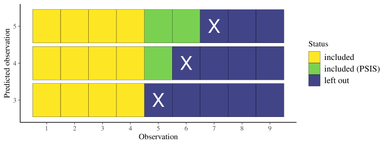
Figure 1: Visualisation of PSIS approximated one-step-ahead predictions. Predicted observations are indicated by X. In the shown example, the model was last refit at the $i^{\star}=4$th observation.

Instead of moving forward in time, it is also possible to do PSIS-LFO-CV moving backwards in time. However, in that case the target posterior is approximated by a distribution based on more observations and, as such, the proposal distribution is narrower than the target. This can result in highly influential importance weights more often than when the proposal is wider than the target, which is the case for the forward PSIS-LFO-CV described above. In Appendix B, we show that moving backwards indeed requires more refits than moving forward, and without any increase in accuracy. When we refer to the PSIS-LFO-CV algorithm in the main text we are referring to the forward version.

The threshold $\tau$ is crucial to the accuracy and speed of the PSIS-LFO-CV algorithm. If $\tau$ is too large then we need fewer refits but accuracy will suffer. If $\tau$ is too small then accuracy will be higher but many refits will be required and the computation time may be impractical. Limiting the number of refits without sacrificing too much accuracy is essential since almost all of the computation time for exact cross-validation of Bayesian models is spent fitting the models (not calculating the predictions). Therefore, any reduction we can achieve in the number of refits essentially implies a proportional reduction in the overall time required for cross-validation of Bayesian models. We will come back to the issue of setting appropriate thresholds in Section 3.

3 Simulations

To evaluate the quality of the PSIS-LFO-CV approximation, we performed a simulation study in which the following conditions were systematically varied:

• The number $M$ of future observations to be predicted took on values of $M=1$ and $M=4$.

• The threshold $\tau$ of the Pareto $k$ estimates was varied between $k=0.5$ to $k=0.7$ in steps of $0.1$.

• Six different data generating models were evaluated, with linear and/or quadratic terms and/or autoregressive terms of order 2 (see Figure 2 for an illustration).

In all cases the time series consisted of $N=200$ observations and the minimal number of observations required before make predictions was set to $L=25$. We ran $100$ simulation trials per condition.

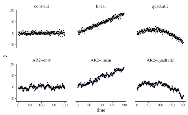
Figure 2: Illustration of the models used in the simulations. Black points are observed data. The blue line represents posterior predictions of the model resembling the true data-generating process with 90% prediction intervals shown in gray. More details are provided in the text.

Autoregressive (AR) models are some of the most commonly used time series models. An AR(p) model – an autoregressive model of order $p$ – can be defined as

$$y_{i}=\eta_{i}+\varepsilon_{i}\quad\text{with}\quad\varepsilon_{i}=\sum_{k=1}^{p}\varphi_{k}\varepsilon_{i-k}+e_{i},$$ (11)

where $\eta_{i}$ is the linear predictor for the $i$th observation, $\varphi_{k}$ are the autoregressive parameters on the residuals $\varepsilon_{i}$, and $e_{i}$ are pairwise independent errors, which are usually assumed to be normally distributed with equal variance $\sigma^{2}$. The model implies a recursive formula that allows for computing the right-hand side of the equation for observation $i$ based on the values of the equations computed for previous observations. Observations from an AR process are therefore not conditionally independent by definition, but the likelihood still factorizes because we can write down a separate contribution for each observation (see Bürkner et al.,, 2020, for more discussion on factorizability of statistical models).

In the quadratic model with AR(2) effects (the most complex model in our simulations), the true data generating process was defined as

$$y_{i}=b_{0}+b_{1}t+b_{2}t^{2}+\varepsilon_{i}\quad\text{with}\quad\varepsilon_{i}=\varphi_{1}\varepsilon_{i-1}+\varphi_{2}\varepsilon_{i-2}+e_{i},$$ (12)

where $t$ is the time variable scaled to the unit interval, that is, $t=0$ for the smallest time point ($1$ in our simulations) and $t=1$ for the largest time point ($200$ in our simulations). Specifically, we set the true regression coefficients to the values of $b_{0}=0$, $b_{1}=17$, $b_{2}=25$, and the true autocorrelation parameters to $\varphi_{1}=0.5$, and $\varphi_{2}=0.3$ (see Figure 2 for an illustration). The choices of the regression coefficients were done so that neither the linear nor quadratic term dominates the other within the specified time frame. The values of the autocorrelation parameters were set to represent typical positively autocorrelated data. In the simulation conditions without linear and/or quadratic and/or AR(2) terms, the corresponding true parameters were simply fixed to zero. We always fit the true data generating model to the data. This is neither required for the validity of LFO-CV in general nor for the validity of the comparison between exact and approximate versions but simply a choice of convenience. For example, a linear model without autocorrelation is used when all but $b_{0}$ and $b_{1}$ were set to zero in the simulations.

In addition to exact and approximate LFO-CV, we also computed approximate LOO-CV for comparison. This is not because we think LOO-CV is a generally appropriate approach for time series models, but because, in the absence of any approximate LFO-CV method, researchers may have used approximate LOO-CV for time series models in the past simply because it was the only available option. Demonstrating that LOO-CV is a biased estimate of LFO-CV underscores the importance of developing methods better suited for the task.

All simulations were done in R (R Core Team,, 2018) using the brms package (Bürkner,, 2017, 2018) together with the probabilistic programming language Stan (Carpenter et al.,, 2017; Stan Development Team,, 2019) for model fitting, the loo R package (Vehtari et al., 2019a, ) for the PSIS computations, and several tidyverse R packages (Wickham,, 2017) for data processing. The full code and all results are available on Github (https://github.com/paul-buerkner/LFO-CV-paper).

3.1 Results

In this section we focus on the ELPD as a measure out-of-sample predictive performance for reasons outlined in Section 2. In Appendix C, we provide additional simulation results for the RMSE.

Results of the 1-SAP simulations are visualized in Figure 3. Comparing the columns of Figure 3, it is clearly visible that the the accuracy of the PSIS approximation is independent of the threshold $\tau$ when $\tau$ is within the interval $[0.5,0.7]$ motivated in 2.1.1 (this would not be the case if $\tau$ was allowed to be larger; Vehtari et al., 2019b, ). For all conditions, the PSIS-LFO-CV approximation is highly accurate, that is, both unbiased and low in variance around the corresponding exact LFO-CV value (represented by the dashed line in Figure 3). The proportion of observations at which refitting the model was required did not exceed $3\%$ under any of the conditions and only increased minimally when decreasing $\tau$ (see Table 1). At least for the models investigated in our simulations, using $\tau=0.7$ seems to be sufficient for achieving high accuracy and as such there is no need to lower the threshold below that value. As expected, LOO-CV (the lighter histograms in Figure 3) is a biased estimate of the 1-SAP performance for all non-constant models, in particular for models with a trend in the time series. More precisely, LOO-CV is positively biased, which implies that it systematically overestimates $M$-SAP performance of time series models.

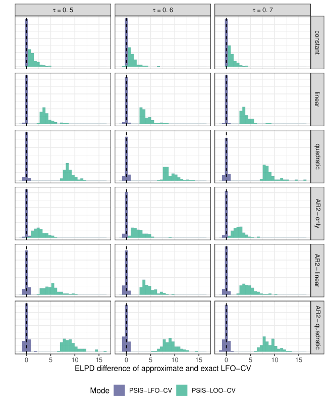
Figure 3: Simulation results of 1-step-ahead predictions. Histograms are based on 100 simulation trials of time series with $N=200$ observations requiring at least $L=25$ observations to make predictions. The black dashed lines indicates the exact LFO-CV result.

Table 1: Mean proportions of required refits for PSIS-LFO-CV.

M	$\tau$	constant	linear	quadratic	AR2-only	AR2-linear	AR2-quadratic
1	0.5	0.01	0.01	0.02	0.01	0.02	0.03
	0.6	0.01	0.01	0.02	0.01	0.02	0.02
	0.7	0.01	0.01	0.02	0.01	0.01	0.02
4	0.5	0.01	0.01	0.02	0.01	0.02	0.03
	0.6	0.01	0.01	0.02	0.01	0.02	0.02
	0.7	0.01	0.01	0.02	0.01	0.01	0.02

• Note: Results are based on 100 simulation trials of time series with $N=200$ observations requiring at least $L=25$ observations to make predictions. Abbreviations: $\tau$ = threshold of the Pareto $k$ estimates; $M$ = number of predicted future observations.

Results of the 4-SAP simulations are visualized in Figure 4. Comparing the columns of Figure 4, it is again clearly visible that the accuracy of the PSIS approximation is independent of the threshold $\tau$. The proportion of observations at which refitting the model was required did not exceed $3\%$ under any condition and only increased minimally when decreasing $\tau$ (see Table 1). In light of the corresponding 1-SAP results presented above, this is not surprising because the procedure for determining the necessity of a refit is independent of $M$ (see Section 2.1). PSIS-LOO-CV is not displayed in Figure 4 as the number of observations predicted at each step (4 vs. 1) makes 4-SAP LFO-CV and LOO-CV incomparable.

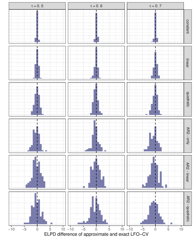
Figure 4: Simulation results of 4-step-ahead predictions. Histograms are based on 100 simulation trials of time series with $N=200$ observations requiring at least $L=25$ observations to make predictions. The black dashed lines indicates the exact LFO-CV result.

4 Case Studies

4.1 Annual measurements of the level of Lake Huron

To illustrate the application of PSIS-LFO-CV for estimating expected $M$-SAP performance, we will fit a model for 98 annual measurements of the water level (in feet) of Lake Huron from the years 1875–1972. This data set is found in the datasets R package, which is installed automatically with R (R Core Team,, 2018). The time series shows rather strong autocorrelation and some downward trend towards lower water levels for later points in time. Figure 5 shows the observed time series of water levels as well as predictions from a fitted AR(4) model.

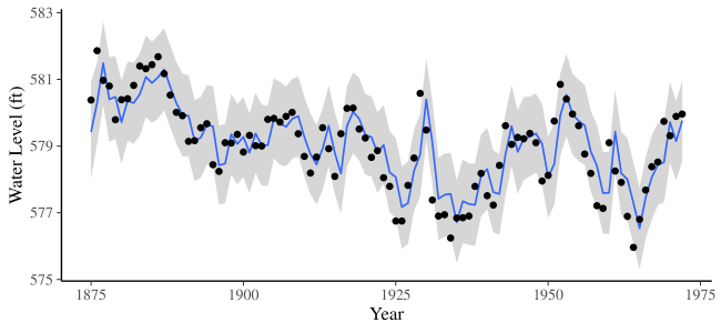
Figure 5: Water Level in Lake Huron (1875-1972). Black points are observed data. The blue line represents mean predictions of an AR(4) model with 90% prediction intervals shown in gray.

Based on this data and model, we will illustrate the use of PSIS-LFO-CV to provide estimates of $1$-SAP and $4$-SAP when leaving out all future values. To allow for reasonable predictions, we will require at least $L=20$ historical observations (20 years) to make predictions. Further, we set a threshold of $\tau=$ 0.7 for the Pareto $k$ estimates that indicate when refitting becomes necessary. Our fully reproducible analysis of this case study can be found on GitHub (https://github.com/paul-buerkner/LFO-CV-paper).

We start by computing exact and PSIS-approximated LFO-CV of 1-SAP. The computed ELPD values are ${\rm ELPD}_{\rm exact}=$ -93.48 and ${\rm ELPD}_{\rm approx}=$ -93.62, which are almost identical. Not only is the overall ELPD estimated accurately but so are all of the pointwise ELPD contributions (see the left panel of Figure 6). In comparison, PSIS-LOO-CV returns ${\rm ELPD}_{\rm loo}=$ -88.9, overestimating the predictive performance and as suggested by our simulation results for stationary autoregressive models (see fourth row of Figure 3). Plotting the Pareto $k$ estimates reveals that the model had to be refit 3 times, out of a total of $N-L=$ 78 predicted observations (see Figure 7). On average, this means one refit every 26.0 observations, which implies a drastic speed increase compared to exact LFO-CV.

Performing LFO-CV for 4-SAP, we obtained ${\rm ELPD}_{\rm exact}=$ -411.41 and ${\rm ELPD}_{\rm approx}=$ -412.78, which are again very similar. In general, as $M$ increases, the approximation will tend to become more variable around the true value in absolute ELPD units because the ELPD increment of each observation will be based on more and more observations (see also Section 3). For this example, we see some considerable differences in the pointwise ELPD contributions of specific observations which were hard to predict accurately by the model (see the right panel of Figure 6). This is to be expected because predicting $M$ steps ahead using an AR model will yield highly uncertain predictions if most of the autocorrelation happens at lags smaller than $M$ (see also the bottom rows in Figure 4). For such a model, it may be ill-advised to evaluate predictions too far into the future, at least when using the approximate methods presented in this paper. Since, for a constant threshold $\tau$, the importance weights are the same independent of $M$, the Pareto $k$ estimates are the same for $4$-SAP and $1$-SAP.

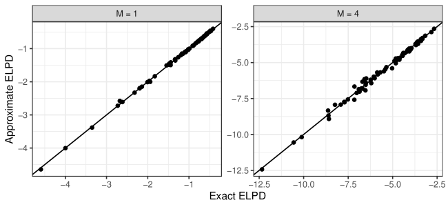
Figure 6: Pointwise exact vs. PSIS-approximated ELPD contributions for 1-SAP (left) and 4-SAP (right) for the Lake Huron model. A threshold of $\tau=0.7$ was used for the Pareto $k$ estimates. $M$ is the number of predicted future observations.

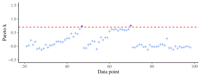
Figure 7: Pareto $k$ estimates for PSIS-LFO-CV of the Lake Huron model. The dotted red line indicates the threshold at which the refitting was necessary.

4.2 Annual date of the cherry blossoms in Japan

The cherry blossom in Japan is a famous natural phenomenon occurring once every year during spring. As the climate changes so does the annual date of the cherry blossom (Aono and Kazui,, 2008; Aono and Saito,, 2010). The most complete reconstruction available to date contains data between 801 AD and 2015 AD (Aono and Kazui,, 2008; Aono and Saito,, 2010) and is available online (http://atmenv.envi.osakafu-u.ac.jp/aono/kyophenotemp4/).

In this case study, we will predict the annual date of the cherry blossom using an approximate Gaussian process model (Solin and Särkkä,, 2014; Riutort Mayol et al.,, 2019) to provide flexible non-linear smoothing of the time series. A visualisation of both the data and the fitted model is provided in Figure 8. While the time series appears rather stable across earlier centuries, with substantial variation across consecutive years, there are some clearly visible trends in the data. Particularly in more recent years, the cherry blossom has tended to happen much earlier than before, which may be a consequence of changes in the climate (Aono and Kazui,, 2008; Aono and Saito,, 2010).

Based on this data and model, we will illustrate the use of PSIS-LFO-CV to provide estimates of $1$-SAP and $4$-SAP leaving out all future values. To allow for reasonable predictions of future values, we will require at least $L=100$ historical observations (100 years) to make predictions. Further, we set a threshold of $\tau=$ 0.7 for the Pareto $k$ estimates to determine when refitting becomes necessary. Our fully reproducible analysis of this case study can be found on GitHub (https://github.com/paul-buerkner/LFO-CV-paper).

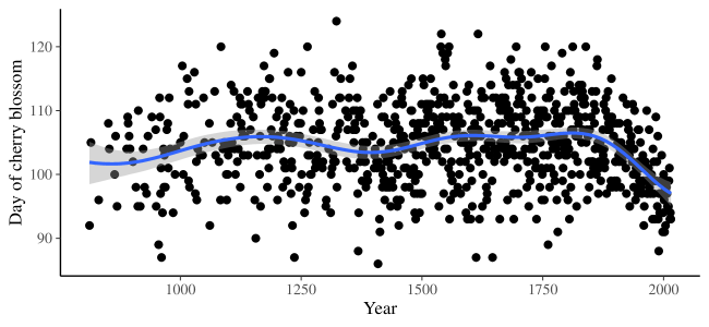
Figure 8: Day of the cherry blossom in Japan (812-2015). Black points are observed data. The blue line represents mean predictions of a thin-plate spline model with 90% regression intervals shown in gray.

We start by computing exact and PSIS-approximated LFO-CV of 1-SAP. We compute ${\rm ELPD}_{\rm exact}=$ -2345.7 and ${\rm ELPD}_{\rm approx}=$ -2344.9, which are highly similar. As shown in the left panel of Figure 9, the pointwise ELPD contributions are highly accurate, with no outliers. The approximation has worked well for all observations. PSIS-LFO-CV performs much better than PSIS-LOO-CV (${\rm ELPD}_{\rm approx}=$ -2340.3), which overestimates the predictive performance. Plotting the Pareto $k$ estimates reveals that the model had to be refit 6 times, out of a total of $N-L=$ 727 predicted observations (see Figure 10). On average, this means one refit every 121.2 observations, which implies a drastic speed increase as compared to exact LFO-CV.

Performing LFO-CV of 4-SAP, we compute ${\rm ELPD}_{\rm exact}=$ -9348.3 and ${\rm ELPD}_{\rm approx}=$ -9345.5, which are again similar but not as close as the corresponding 1-SAP results. This is to be expected as the uncertainty of PSIS-LFO-CV increases for increasing $M$ (see Section 3). As displayed in the right panel of Figure 9, the pointwise ELPD contributions are highly accurate in most cases, with a few small outliers in both directions. For constant threshold $\tau$, the importance weights are the same independent of $M$, so the Pareto $k$ estimates are the same for $4$-SAP and $1$-SAP.

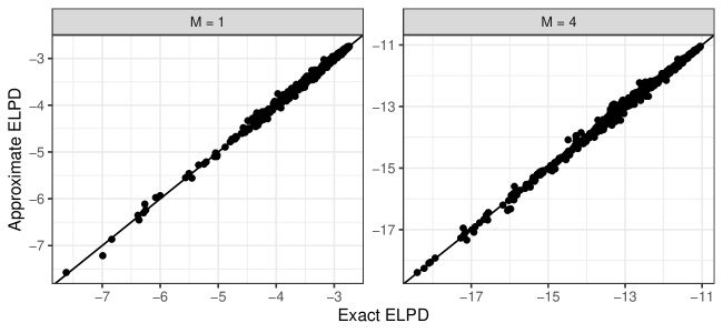
Figure 9: Pointwise exact vs. PSIS-approximated ELPD contributions of 1-SAP (left) and 4-SAP (right) for the cherry blossom model. A threshold of $\tau=0.7$ was used for the Pareto $k$ estimates. $M$ is the number of predicted future observations.

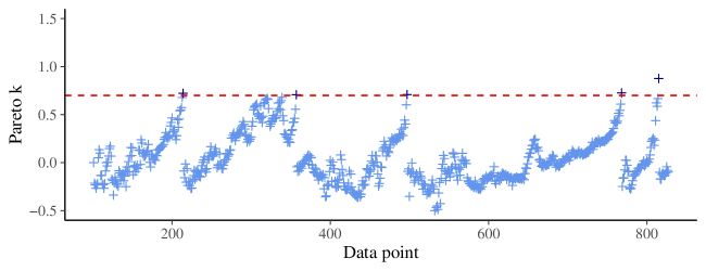
Figure 10: Pareto $k$ estimates for PSIS-LFO-CV of the cherry blossom model. The dotted red line indicates the threshold at which the refitting was necessary.

5 Conclusion

We proposed, evaluated, and demonstrated PSIS-LFO-CV, a method for approximating cross-validation of Bayesian time series models. PSIS-LFO-CV is intended to be used when the prediction task is predicting future values based solely on past values, in which case leave-one-out cross-validation is inappropriate. Within the set of such prediction tasks, we can choose the number $M$ of future observations to be predicted. For a set of common time series models, we established via simulations that PSIS-LFO-CV is an unbiased approximation of exact LFO-CV if we choose the threshold $\tau$ of the Pareto $k$ estimates to not be larger than $\tau=0.7$. That is, PSIS-LFO-CV does not require a smaller (stricter) threshold than PSIS-LOO-CV to achieve satistfactory accuracy.

By nature of the approximated $M$-step-ahead predictions, the computation time of PSIS-LFO-CV still increases linearily with the number of observations $N$. However, in our numerical experiments, we were able to reduce to computation time by a factor of roughly 25 to 100 compared to exact LFO-CV, which is enough to make LFO-CV realistic for many applications.

A limitation of our current approach is that the uncertainty in the approximate LFO-CV estimates is hard to quantify. There are at least three types of uncertainty which could be considered here. First, there is uncertainty induced by approximating exact LFO-CV using (Pareto smoothed) importance sampling. Based on theoretical considerations of the approximation and numerical experiments both presented in Vehtari et al., 2019b , any PSIS approximation will be very close to the exact value as long as the Pareto $k$ diagnostic does not exceed the threshold of $0.7$, which we used as the refit criterion in our approximate LFO-CV approach. Second, there is uncertainty caused by finite amounts of data. For 1-step-ahead predictions, we can use an analogous approach to what is done in approximate LOO-CV by computing the standard error across the pointwise estimates for each observation (Vehtari et al.,, 2017). More generally, for $M$-step-ahead predictions, we can compute the standard error by using every $M$th value which are then independent. Third, there is uncertainty induced by the finite number of posterior draws but this uncertainty tends to be negligable with just a few thousand draws compared to the second source of uncertainty (Vehtari et al.,, 2017). Investigating uncertainty measures for (approximate) LFO-CV in more detail is left for future research.

Lastly, we want to briefly note that LFO-CV can also be used to compute marginal likelihoods. Using basic rules of conditional probability, we can factor the log marginal likelihood as

$$\log p(y)=\sum_{i=1}^{N}\log p(y_{i}\,|\,y_{1:(i-1)}).$$ (13)

This is exactly the ELPD of 1-SAP if we set $L=0$, that is if we choose to predict all observations using their respective past (the very first observation is only predicted from the prior). As such, marginal likelihoods may be approximated using PSIS-LFO-CV. Although this approach is unlikely to be more efficient than methods specialized for computing marginal likelihoods (e.g., bridge sampling; Meng and Wong,, 1996; Meng and Schilling,, 2002; Gronau et al.,, 2017), it may be a noteworthy option if for some reason other methods fail.

6 Acknowledgments

We thank Daniel Simpson, Shira Mitchell, Måns Magnusson, and anonymous reviewers for helpful comments and discussions on earlier versions of this paper. We acknowledge the Academy of Finland (grants 298742, 313122) as well as the Technology Industries of Finland Centennial Foundation (grant 70007503; Artificial Intelligence forResearch and Development) for partial support of this work. We also acknowledge the computational resources provided by the Aalto Science-IT project.

Appendix

Appendix A: Pseudo code for PSIS LFO-CV

The R flavored pseudo code below provides a description of the proposed PSIS-LFO-CV algorithm when leaving out all future values. See https://github.com/paul-buerkner/LFO-CV-paper for the actual R code.

# Approximate Leave-Future-Out Cross-Validation (LFO-CV)

# Arguments:

#   model: the fitted time series model based on the complete data

#   data: the complete data set

#   M: number of steps to be predicted into the future

#   L: minimal number of observations necessary to make predictions

#   tau: threshold of the Pareto-k-values

# Returns:

#   PSIS approximated ELPD value of LFO-CV

PSIS_LFO_CV = function(model, data, M, L, tau) {

  N = number_of_rows(data)

  S = number_of_draws(model)

  out = vector(length = N)

  # refit the model using the first L observations

  i_star = L

  model_star = update(model, data = data[1:L, ])

  out[L] = exact_ELPD(model_star, data = data[(L + 1):(L + M), ])

  # loop over all observations at which to perform predictions

  for (i in (L + 1):(N - M)) {

    PSIS_object = PSIS(model_star, data = data[(i_star + 1):i , ])

    k = pareto_k_values(PSIS_object)

    if (k > tau) {

      # refitting the model is necessary

      i_star = i

      model_star = update(model_star, data = data[1:i, ])

      out[i] = exact_ELPD(model_star, data = data[(i + 1):(i + M), ])

    } else {

      # PSIS approximation is possible

      log_PSIS_weights = log_weights(PSIS_object)

      out[i] = approx_ELPD(model_star, data = data[(i + 1):(i + M), ],

                           log_weights = log_PSIS_weights)

    }

  }

  return(sum(out))

}

Appendix B: Backward PSIS-LFO-CV

Instead of moving forward in time, that is, starting our predictions from the $L$th observation, we may also move backwards, a procedure to which we will refer to as backward PSIS-LFO-CV. Starting with $i=N-M$, we approximate each $p(y_{i+1:M}\,|\,y_{1:i})$ via

$$p(y_{i+1:M}\,|\,y_{1:i})\approx\frac{\sum_{s=1}^{S}w_{i}^{(s)}\,p(y_{i+1:M}\,|\,y_{1:i},\theta^{(s)})}{\sum_{s=1}^{S}w_{i}^{(s)}},$$ (14)

where $w_{i}^{(s)}$ are the PSIS weights and $\theta^{(s)}=\theta^{(s)}_{1:i^{\star}}$ are draws from the posterior distribution based on the first $1:i^{\star}$ observations. In backward LFO-CV, we start using the model based on all observations, that is, set $i^{\star}=N$. To obtain $w_{i}^{(s)}$, we first compute the raw importance ratios

$$r_{i}^{(s)}=r_{i}(\theta^{(s)})=\frac{f_{1:i}(\theta^{(s)})}{f_{1:i^{\star}}(\theta^{(s)})}\propto\frac{p(\theta^{(s)})\prod_{j\in 1:i}p(y_{j}\,|\,y_{1:(j-1)},\theta^{(s)})}{p(\theta^{(s)})\prod_{j\in 1:i^{\star}}p(y_{j}\,|\,y_{1:(j-1)},\theta^{(s)})}=\frac{1}{\prod_{j\in(i+1):i^{\star}}p(y_{j}\,|\,y_{1:(j-1)},\theta^{(s)})},$$ (15)

and then stabilize them using PSIS as described in Section 2.1.1. The function $f_{1:i}$ denotes the posterior distribution based on the first $i$ observations, that is, $f_{1:i}=p(\theta\,|\,y_{1:i})$, with $f_{1:i^{\star}}$ defined analogously. The index set $(i+1):i^{\star}$ indicates all observations which are part of the data for the actually fitted model $f_{1:i^{\star}}$ but not for the model $f_{1:i}$ whose predictive performance we are trying to approximate. The proportional statement arises from the fact that we ignore the normalizing constants $p(y_{1:i})$ and $p(y_{1:i^{\star}})$ of the compared posteriors, which leads to a self-normalized variant of PSIS (c.f. Vehtari et al.,, 2017). This approach to computing importance ratios is a generalization of the approach used in PSIS-LOO-CV, where only a single observation is left out at a time.

Starting from $i=N-M$, we gradually decrease $i$ by $1$ (i.e., we move backwards in time) and repeat the process. At some observation $i$, the variability of the importance ratios $r_{i}^{(s)}$ will become too large and importance sampling fails. We will refer to this particular value of $i$ as $i^{\star}_{1}$. To identify the value of $i^{\star}_{1}$, we check for which value of $i$ does the estimated shape parameter $k$ of the generalized Pareto distribution first cross a certain threshold $\tau$ (Vehtari et al., 2019b, ). Only then do we refit the model using only observations up to $i^{\star}_{1}$ by setting $\theta^{(s)}=\theta^{(s)}_{1:i^{\star}_{1}}$ as well as $i^{\star}=i^{\star}_{1}$ and restarting the process. An illustration of this procedure is shown in Figure 11. In some cases we may only need to refit once and in other cases we will find a value $i^{\star}_{2}$ that requires a second refitting, maybe an $i^{\star}_{3}$ that requires a third refitting, and so on. We repeat the refitting as many times as is required (only if $k>\tau$) until we arrive at $i=L$. Recall that $L$ is the minimum number of observations we have deemed acceptable for making predictions.

In forward PSIS-LFO-CV, we have seen a threshold of $\tau=0.7$ to be sufficient for achieving satisfactory accuracy. For backward PSIS-LFO-CV, $\tau$ likely has to be smaller. More precisely, we can expect an appropriate threshold for the backward mode to be somewhere between $0.5\leq\tau\leq 0.7$. It is unlikely to be as high as the $\tau=0.7$ default used for PSIS-LOO-CV because there will be more dependence in the errors in the case of backward PSIS-LFO-CV. If there is a large error when leaving out the $i$th observation, then there is likely to also be a large error when leaving out observations $i,i-1,i-2,\ldots$ until a refit is performed. This means that highly influential observations (ones with a large $k$ estimate) are likely to have stronger effects on the total estimate for backward LFO-CV than for LOO-CV.

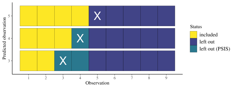
Figure 11: Visualisation of approximate one-step-ahead predictions using backward PSIS-LFO-CV. Predicted observations are indicated by X. In the shown example, the model was last refit at the $i^{\star}=4$th observation.

The simulation results comparing backward to forward PSIS-LFO-CV can be found in Figure 12 for $1$-SAP and in Figure 13 for $4$-SAP. As visible in both figures, backward PSIS-LFO-CV requires a lower $\tau$ threshold than forward PSIS-LFO-CV in order to be accurate ($\tau=0.6$ vs. $\tau=0.7$). Otherwise, it may have a small positive bias. Further, as can be seen in Table 2, backward PSIS-LFO-CV requires considerably more refits then forward PSIS-LFO-CV. Together, this indicates that, in expectation, backward PSIS-LFO-CV is inferior to forward PSIS-LFO-CV.

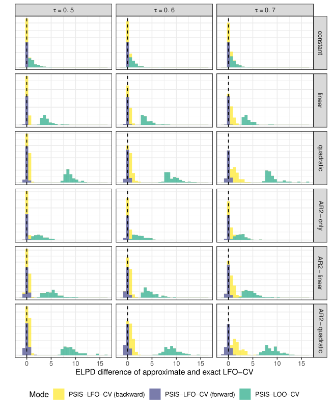
Figure 12: Simulation results of 1-step-ahead predictions for both forward and backward PSIS-LFO-CV. Histograms are based on 100 simulation trials of time series with $N=200$ observations requiring at least $L=25$ observations to make predictions. The black dashed lines indicates the exact LFO-CV result.

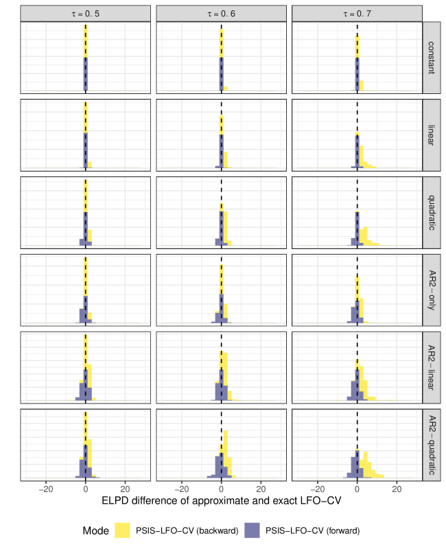
Figure 13: Simulation results of 4-step-ahead predictions for both forward and backward PSIS-LFO-CV. Histograms are based on 100 simulation trials of time series with $N=200$ observations requiring at least $L=25$ observations to make predictions. The black dashed lines indicates the exact LFO-CV result.

Table 2: Mean proportions of required refits for both forward and backward PSIS-LFO-CV.

Mode	M	$\tau$	constant	linear	quadratic	AR2-only	AR2-linear	AR2-quadratic
backward	1	0.5	0.03	0.08	0.17	0.04	0.09	0.18
		0.6	0.02	0.06	0.12	0.03	0.06	0.12
		0.7	0.01	0.04	0.09	0.02	0.04	0.08
	4	0.5	0.03	0.08	0.17	0.04	0.09	0.18
		0.6	0.02	0.06	0.12	0.03	0.06	0.12
		0.7	0.01	0.04	0.09	0.02	0.04	0.09
forward	1	0.5	0.01	0.01	0.02	0.01	0.02	0.03
		0.6	0.01	0.01	0.02	0.01	0.02	0.02
		0.7	0.01	0.01	0.02	0.01	0.01	0.02
	4	0.5	0.01	0.01	0.02	0.01	0.02	0.03
		0.6	0.01	0.01	0.02	0.01	0.02	0.02
		0.7	0.01	0.01	0.02	0.01	0.01	0.02

• Note: Results are based on 100 simulation trials of time series with $N=200$ observations requiring at least $L=25$ observations to make predictions. Abbreviations: $\tau$ = threshold of the Pareto $k$ estimates; $M$ = number of predicted future observations.

We may even combine forward and backward mode PSIS-LFO-CV in the following way. First, we start with forward mode until a refit becomes necessary, say at observation $i^{\star}$. Then, we apply backward mode on the basis of the refitted model and perform multiple proposal importance sampling (Veach and Guibas,, 1995; He and Owen,, 2014) to obtain the ELPD values of the observations $i^{\star}-1,i^{\star}-2,\ldots$ from the mixture of the forward and backward distributions. We do this until the backward mode requires a refit at which point we stop the process and continue with forward mode at observation $i^{\star}$. This algorithm requires exactly as many refits as the forward mode while potentially increasing accuracy for those observations for which the pointwise ELPD contribution was computed via both forward and backward mode PSIS-LFO-CV. In the present paper, we did not investigate the possibility of multiple importance sampling in more detail, but it could be a promising extention to be studied in the future.

Appendix C: PSIS-LFO-CV for the RMSE

We may also use other measures of predictive performance than the ELPD, for instance the RMSE. For a scalar response $y$ and corresponding vector $\hat{y}$ of a total of $S$ posterior predictions $\hat{y}^{(s)}$, the RSME is defined as

$$\text{RMSE}(y,\hat{y})=\frac{1}{S}\sum_{s=1}^{S}(\hat{y}^{(s)}-y)^{2}.$$ (16)

If we predict multiple responses in the future (i.e., perform $M$-SAP with $M>1$), we simply sum the RMSE over all those responses. When approximating the RMSE via PSIS, we use the (Pareto smoothed) importance weights $w^{(s)}$ (see Section 2.1.2) to estimate

$$\text{RMSE}(y,\hat{y})\approx\frac{\sum_{s=1}^{S}w^{(s)}(\hat{y}^{(s)}-y)^{2}}{\sum_{s=1}^{S}w^{(s)}}.$$ (17)

The remaining computations are analogous to using the ELPD as a measure of predictive performance in LFO-CV and so we do not spell out the details here. The code we provide on GitHub (https://github.com/paul-buerkner/LFO-CV-paper) is modularized and also has an implementation of the (approximate) RMSE for LFO-CV.

Results of the 1-SAP and 4-SAP RMSE simulations are visualized in Figure 14 and 15, respectively. It is clearly visible that the the accuracy of the PSIS RMSE approximation is nearly independent of the threshold $\tau$ when $\tau$ is within the interval $[0.5,0.7]$ motivated in 2.1.1 (this would not be the case if $\tau$ was allowed to be larger; Vehtari et al., 2019b, ). For all conditions, the PSIS-LFO-CV approximation is highly accurate, that is, both approximately unbiased and low in variance around the corresponding exact LFO-CV RMSE value (represented by the dashed line in Figure 3). Taken together, these simulations indicate that PSIS-LFO-CV not only works well with the ELPD but also with the RMSE.

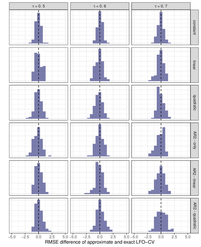
Figure 14: Simulation results of 1-step-ahead predictions using the RMSE as measure of predictive accuracy. Histograms are based on 100 simulation trials of time series with $N=200$ observations requiring at least $L=25$ observations to make predictions. The black dashed lines indicates the exact LFO-CV result.

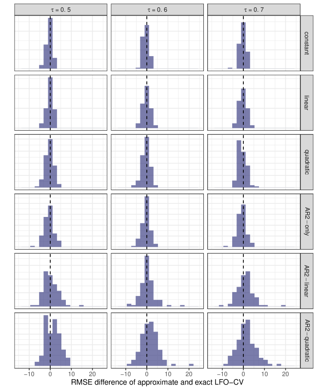
Figure 15: Simulation results of 4-step-ahead predictions using the RMSE as measure of predictive accuracy. Histograms are based on 100 simulation trials of time series with $N=200$ observations requiring at least $L=25$ observations to make predictions. The black dashed lines indicates the exact LFO-CV result.

References

- Ando and Tsay, (2010) Ando, T. and Tsay, R. (2010). Predictive likelihood for Bayesian model selection and averaging. International Journal of Forecasting, 26(4):744–763.
- Andrieu et al., (2010) Andrieu, C., Doucet, A., and Holenstein, R. (2010). Particle markov chain monte carlo methods. Journal of the Royal Statistical Society: Series B (Statistical Methodology), 72(3):269–342.
- Aono and Kazui, (2008) Aono, Y. and Kazui, K. (2008). Phenological data series of cherry tree flowering in Kyoto, Japan, and its application to reconstruction of springtime temperatures since the 9th century. International Journal of Climatology: A Journal of the Royal Meteorological Society, 28(7):905–914.
- Aono and Saito, (2010) Aono, Y. and Saito, S. (2010). Clarifying springtime temperature reconstructions of the medieval period by gap-filling the cherry blossom phenological data series at Kyoto, Japan. International journal of biometeorology, 54(2):211–219.
- Bernardo and Smith, (1994) Bernardo, J. M. and Smith, A. F. (1994). Bayesian theory, volume 405. John Wiley & Sons.
- Bingham et al., (2019) Bingham, E., Chen, J. P., Jankowiak, M., Obermeyer, F., Pradhan, N., Karaletsos, T., Singh, R., Szerlip, P., Horsfall, P., and Goodman, N. D. (2019). Pyro: Deep universal probabilistic programming. The Journal of Machine Learning Research, 20(1):973–978.
- Brockwell et al., (2002) Brockwell, P. J., Davis, R. A., and Calder, M. V. (2002). Introduction to time series and forecasting, volume 2. Springer.
- Bürkner, (2017) Bürkner, P.-C. (2017). brms: An R package for Bayesian multilevel models using Stan. Journal of Statistical Software, 80(1):1–28.
- Bürkner, (2018) Bürkner, P.-C. (2018). Advanced Bayesian multilevel modeling with the R package brms. The R Journal, pages 395–411.
- Bürkner et al., (2020) Bürkner, P.-C., Gabry, J., and Vehtari, A. (2020). Efficient leave-one-out cross-validation for bayesian non-factorized normal and student-t models.
- Carpenter et al., (2017) Carpenter, B., Gelman, A., Hoffman, M., Lee, D., Goodrich, B., Betancourt, M., Brubaker, M. A., Guo, J., Li, P., and Ridell, A. (2017). Stan: A probabilistic programming language. Journal of Statistical Software.
- Doucet et al., (2000) Doucet, A., Godsill, S., and Andrieu, C. (2000). On sequential monte carlo sampling methods for bayesian filtering. Statistics and computing, 10(3):197–208.
- Geisser and Eddy, (1979) Geisser, S. and Eddy, W. F. (1979). A predictive approach to model selection. Journal of the American Statistical Association, 74(365):153–160.
- Gordon et al., (1993) Gordon, N. J., Salmond, D. J., and Smith, A. F. (1993). Novel approach to nonlinear/non-gaussian bayesian state estimation. In IEE proceedings F (radar and signal processing), volume 140, pages 107–113. IET.
- Gronau et al., (2017) Gronau, Q. F., Sarafoglou, A., Matzke, D., Ly, A., Boehm, U., Marsman, M., Leslie, D. S., Forster, J. J., Wagenmakers, E.-J., and Steingroever, H. (2017). A tutorial on bridge sampling. Journal of mathematical psychology, 81:80–97.
- Hamilton, (1994) Hamilton, J. D. (1994). Time series analysis, volume 2. Princeton University Press.
- He and Owen, (2014) He, H. Y. and Owen, A. B. (2014). Optimal mixture weights in multiple importance sampling. arXiv preprint arXiv:1411.3954.
- Hoeting et al., (1999) Hoeting, J. A., Madigan, D., Raftery, A. E., and Volinsky, C. T. (1999). Bayesian model averaging: a tutorial. Statistical science, pages 382–401.
- Kitagawa, (1996) Kitagawa, G. (1996). Monte carlo filter and smoother for non-gaussian nonlinear state space models. Journal of computational and graphical statistics, 5(1):1–25.
- Meng and Schilling, (2002) Meng, X.-L. and Schilling, S. (2002). Warp bridge sampling. Journal of Computational and Graphical Statistics, 11(3):552–586.
- Meng and Wong, (1996) Meng, X.-L. and Wong, W. H. (1996). Simulating ratios of normalizing constants via a simple identity: a theoretical exploration. Statistica Sinica, pages 831–860.
- Murray and Schön, (2018) Murray, L. M. and Schön, T. B. (2018). Automated learning with a probabilistic programming language: Birch. Annual Reviews in Control.
- Plummer et al., (2003) Plummer, M. et al. (2003). Jags: A program for analysis of bayesian graphical models using gibbs sampling. In Proceedings of the 3rd international workshop on distributed statistical computing, volume 124. Vienna, Austria.
- R Core Team, (2018) R Core Team (2018). R: A Language and Environment for Statistical Computing. R Foundation for Statistical Computing, Vienna, Austria.
- Riutort Mayol et al., (2019) Riutort Mayol, G., Andersen, M. R., Bürkner, P., and Vehtari, A. (2019). Hilbert space methods to approximate Gaussian processes using Stan. In preparation.
- Salvatier et al., (2016) Salvatier, J., Wiecki, T. V., and Fonnesbeck, C. (2016). Probabilistic programming in python using PyMC3. PeerJ Computer Science, 2:e55.
- Solin and Särkkä, (2014) Solin, A. and Särkkä, S. (2014). Hilbert space methods for reduced-rank Gaussian process regression. arXiv preprint arXiv:1401.5508.
- Stan Development Team, (2019) Stan Development Team (2019). RStan: the R interface to Stan. R package version 2.19.1.
- Veach and Guibas, (1995) Veach, E. and Guibas, L. J. (1995). Optimally combining sampling techniques for monte carlo rendering. In Proceedings of the 22nd annual conference on Computer graphics and interactive techniques, pages 419–428. ACM.
- (30) Vehtari, A., Gabry, J., Yao, Y., and Gelman, A. (2019a). loo: Efficient leave-one-out cross-validation and WAIC for Bayesian models. R package version 2.1.0.
- Vehtari et al., (2017) Vehtari, A., Gelman, A., and Gabry, J. (2017). Practical Bayesian model evaluation using leave-one-out cross-validation and WAIC. Statistics and Computing, 27(5):1413–1432.
- Vehtari and Lampinen, (2002) Vehtari, A. and Lampinen, J. (2002). Bayesian model assessment and comparison using cross-validation predictive densities. Neural computation, 14(10):2439–2468.
- Vehtari and Ojanen, (2012) Vehtari, A. and Ojanen, J. (2012). A survey of Bayesian predictive methods for model assessment, selection and comparison. Statistics Surveys, 6:142–228.
- (34) Vehtari, A., Simpson, D., Gelman, A., Yao, Y., and Gabry, J. (2019b). Pareto smoothed importance sampling. arXiv preprint.
- Wickham, (2017) Wickham, H. (2017). tidyverse: Easily Install and Load the ’Tidyverse’. R package version 1.2.1.
- Yao et al., (2018) Yao, Y., Vehtari, A., Simpson, D., and Gelman, A. (2018). Using stacking to average Bayesian predictive distributions (with discussion). Bayesian Analysis, 13(3):917–1003.