Osmosis, from molecular insights to large-scale applications
	Sophie Marbacha,† and Lydéric Bocqueta,∗
	Osmosis is a universal phenomenon occurring in a broad variety of processes and fields. It is the archetype of entropic forces, both trivial in its fundamental expression – the van ’t Hoff perfect gas law – and highly subtle in its physical roots. While osmosis is intimately linked with transport across membranes, it also manifests itself as an interfacial transport phenomenon: the so-called diffusio-osmosis and -phoresis, whose consequences are presently actively explored for example for the manipulation of colloidal suspensions or the development of active colloidal swimmers. Here we give a global and unifying view of the phenomenon of osmosis and its consequences with a multi-disciplinary perspective. Pushing the fundamental understanding of osmosis allows one to propose new perspectives for different fields and we highlight a number of examples along these lines, for example introducing the concepts of osmotic diodes, active separation and far from equilibrium osmosis, raising in turn fundamental questions in the thermodynamics of separation. The applications of osmosis are also obviously considerable and span very diverse fields. Here we discuss a selection of phenomena and applications where osmosis shows great promises: osmotic phenomena in membrane science (with recent developments in separation, desalination, reverse osmosis for water purification thanks in particular to the emergence of new nanomaterials); applications in biology and health (in particular discussing the kidney filtration process); osmosis and energy harvesting (in particular, osmotic power and blue energy as well as capacitive mixing); applications in detergency and cleaning, as well as for oil recovery in porous media.

1 Introduction

From the etymological point of view, osmosis denotes a “push” and indeed osmosis is usually associated with the notion of force and pressure. Osmosis is a very old topic, it was first observed centuries ago with reports by Jean-Antoine Nollet in the 18^th century. It was rationalized more than one century later by van ’t Hoff, who showed that the osmotic pressure took the form of a perfect gas equation of state. In practice, an osmotic pressure is typically expressed across a semi-permeable membrane, e.g. a membrane that allows only the solvent to pass while retaining solutes. If two solutions of a liquid containing different solute concentrations are put into contact through such a semi-permeable membrane, the fluid will undergo a driving force pushing it towards the reservoir with the highest solute concentration, see Fig. 1. Reversely, in order to prevent the fluid from passing through the membrane, a pressure has to be applied to the fluid to counteract the flow: the applied pressure is then equal to the osmotic pressure.

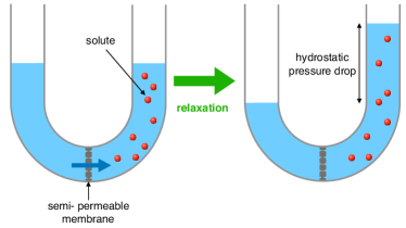
Fig.  1: : Key manifestation of osmosis. A semi-permeable membrane allows transport of water upon a solute concentration difference (in red). The flow of water is directed from the fresh water reservoir to the concentrated reservoir.

Osmosis is therefore extremely simple in its expression. Yet it is one of the most subtle physics phenomenon in its roots – it resulted in many debates over years ^{1, 2}. Osmosis also implies subtle phenomena, in particular as a prototypical illustration for the explicit conversion of entropy of mixing into mechanical work. In spite of centuries of exploration, osmosis as a field remains very lively, with a number of recent breakthroughs both in its concepts and applications as we shall explore in this review. A simple reason for the importance of osmosis is that it is a very powerful phenomenon: giving just one illustrative number, it is amazing to realize that a concentration difference of $\sim 1.2$ molar, which corresponds roughly to the difference between sea and fresh water (and can be easily achieved in anyone’s kitchen), yields an osmotic pressure of $\sim$ 30 atmospheres. This is the hydrostatic pressure felt under a 300m water column ! Osmosis has potentially a destructive power, in particular in soft tissues and membranes, with possible fatal consequences ³. This explains actually why it is also an efficient asset for food preservation (such as fish and meat curing with dry salt).

Osmosis is accordingly also a key and universal phenomenon occurring in many processes, ranging from biological transport in plants, trees and cells, to water filtration, reverse and forward osmosis, energy harvesting and osmotic power, capacitive mixing, oil recovery, detergency and cleaning, active matter, to quote just a few.

The litterature on osmosis and its consequences is accordingly absolutely huge , and it may seem hopeless to cover in a single review all aspects of the topic with an exhaustive discussion of all possible applications. Also, such a comprehensive list would probably be useless for readers who want to catch up with the topics related to osmosis. In writing this review, we thus decided to rather present a tutorial and unified perspective of osmosis, obviously with personal views, avoiding exhaustiveness to highlight a number of significant questions discussed in the recent literature. The review will therefore explore the fundamental foundations of osmosis, emphasizing in particular the – sometimes subtle – mechanical balance at play; then report on more recent concepts and applications related to osmosis which - in our opinion - prove promising for future perspectives. We will accordingly put in context phenomena like diffusio-osmosis and -phoresis, as well as “active” (non-equilibrium) counterparts of osmosis, which were realized lately to play a growing role in numerous applications in filtration and energy harvesting.

The review is organized as follows. We start with some basic reminder of the fundamentals of osmosis in terms of equilibrium and non-equilibrium thermodynamics of the underlying process. We further highlight simplistic views clarifying the mechanical aspects of osmosis. We then discuss membrane-less osmosis and the so-called diffusio-osmotic flows. We then show how such phenomena may be harnessed to go beyond the simple views of van ’t Hoff. We then explore the transport of particles under solute gradients, diffusio-phoresis, and discuss how this phenomenon can be harnessed to manipulate colloidal assemblies. And we finally illustrate a number of applications for the introduced concepts, from desalination, water treatment, the functioning of the kidney, blue energy harvesting, etc. We conclude with some final, brief, perspectives.

2 Osmosis : the van ’t Hoff legacy

2.1 A quick history of osmosis

We start this review with a short and non-exhaustive journey through time in order to highlight how a complete understanding of osmosis emerged over time. We refer e.g. to Ref.4 for a more detailed historical review. The first occurence of the term "osmosis" and clear observation of its effects – beyond the seminal work of Nollet – is reported at least as early as in the works of Henri Dutrochet in the 1820s ^{5, 6}. He observed swelling events or emptying of pockets driven by the presence of various dissolved components in water (different sugars in plants, sperm in slugs…). In reference to the greek term "osmose" (meaning "impulsion" or "push") he introduced the vocabulary "endosmose" and "exosmose". Interestingly, Dutrochet served as a pioneer in linking these different topics by claiming that the same physical force could be used to describe all these events ⁵, which is indeed a unique and fascinating feature of osmosis. Yet, the mechanisms driving osmotic flow were still unclear, and entangled (or believed to be entangled) with capillary and electrical effects. In 1854 T. Graham introduced the word "osmosis" building on the work of Dutrochet ⁷.

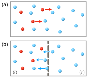
Fig.  2: : Osmosis versus diffusion. (a) situation where motion of the red solute particles is governed by diffusion alone (b) osmosis situation, where motion of the blue solvent particles is driven by osmosis; the solute particles being "repelled" by the membrane, the membrane exerts an effective force on the liquid (solute + solvent) that drives solvent flow towards the highly concentrated reservoir.

Interestingly, the distinction between osmosis and pure diffusion – without a membrane, see Fig. 2 – is not clear from the beginning. The confusion will grow stronger with the work of Adolf Fick in 1855 ⁸, where he claims that diffusive motion (Fickian diffusion) is the driver for osmotic flow (the water concentration imbalance between the two compartments drives the water flow). The question of finding whether osmotic flow is diffusion-driven or not will be an ongoing debate for a century. That diffusion alone cannot account for osmosis is not widely appreciated. In 1957, the debate is definitely closed by an experimental visualization of water flow, using radioactively labeled water molecules ⁹ and verified in Ref.10. The flows measured were significantly higher than that expected by pure diffusion.

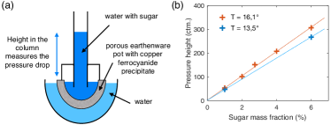
Fig.  3: : First measurements of osmotic pressure.(a) Schematic of a Pfeffer cell, the device used by W. Pfeffer to perform the first measurements of osmotic pressure; (b) Osmotic pressure as a function of solute concentration at two temperatures, with experimental data points from W. Pfeffer ¹¹ verifying a linear relation (the lines are a guide for the eye).

In 1877, Wilhelm Pfeffer made the first measurements of osmotic pressure ¹¹, see Fig. 3. At equilibrium, he measured a rise in the concentrated solution, corresponding to a hydraulic pressure drop that is equal to the osmotic pressure. He measured a linear relation between the osmotic pressure and the concentration difference. But also, Pfeffer measured that for each degree rise in temperature, the pressure would go up by 1/270 ¹². This fact was reported to Jacobus Henricus van ’t Hoff by the botanist Hugo de Vries and van ’t Hoff immediately recognized that 270 was an approximation of 273 K. Intrigued by this result, he attempted in 1887 to rationalize this linear dependence ¹³ and suggested to interpret that the osmotic pressure $\Delta\Pi$ was exerted by the solute particles and equal to the partial pressure that they would have in gas phase (therefore the term "osmotic pressure"):

[…] it occurred to me that with the semipermeable barrier all the reversible transformations that so materially ease the application of thermodynamics to gases, become equally available for solutions… That was a ray of light; and led at once to the inescapable conclusion that the osmotic pressure of dilue solutions must vary with temperature entirely as does gas pressure […]. ¹²

then writing

$$\Delta\Pi=k_{B}T\Delta c_{s}$$ (1)

with $k_{B}$ the Boltzmann constant, $T$ temperature and $\Delta c_{s}$ the solute imbalance between reservoirs.

Eq. (1) is today referred to as the van ’t Hoff law, and gives in practice good agreement for the osmotic pressure measured between two solutions separated by a membrane permeable only to the solvent. For a solute imbalance of $\Delta C_{s}=1.2$ mol.L^-1 (corresponding to the ionic strength difference between fresh and sea water, which is twice – two ions for salt – the typical concentration 0.6 mol.L^-1), we find an osmotic pressure of $\Delta\Pi=k_{B}T\Delta C_{s}\mathcal{N}_{A}\simeq 30$ bar.

At the time, the interpretation of van ’t Hoff gave rise to a number of debates ^{1, 2}. In the following decades a great number of theories were invented to describe the osmotic phenomenon and a detailed review of these theories can be found in Ref.14. Among all these theories, two of them caught a lot of attention. One of them was the proof of van ’t Hoff’s law using the kinetic theory of gas to describe the two solutions ¹⁵ (which was later improved for multicomponent systems ¹⁶). The other one is acknowledged today as the common description of osmosis, and makes use of the concept of chemical potentials first introduced by Josiah Willard Gibbs ¹⁷ (actually introduced as a physical descriptor required to understand osmosis), that we recall in the next section.

2.2 Thermodynamic equilibrium

We start with the thermodynamic derivation of the osmotic pressure as proposed by Gibbs. We follow here the clear-cut presentation proposed in the textbook by Callen ¹⁸, which we recall here for the purpose of settling properly the foundations. In addition to Callen it is also worth reading the rigorous thermodynamic treatment by Guggenheim ¹⁹. We consider a composite system made of two simple reservoirs (left and right) separated by a rigid wall permeable to component $w$ (usually the solvent) and totally impermeable to all other components (labelled $s_{1}$, $s_{2}$ and so on). The whole system is in contact with a thermal bath at temperature $T$. The solvent is in equilibrium over the whole system, i.e. over the two reservoirs, while solutes cannot equilibrate between the reservoirs. Due to the imbalance of solute fraction between both reservoirs, the solvent cannot keep a homogeneous pressure across the two reservoirs while ensuring the equality of chemical potential at equilibrium. An (osmotic) pressure drop builds up, which the membrane withstands.

Assuming that the solute concentration is dilute, the Gibbs free energy of a binary system of solvent and dilute solute can be written as

$$\begin{split}G(T,p,N_{w},N_{s_{1}})=&N_{w}\mu_{w}^{0}(p,T)+N_{s}\mu_{s}^{0}(p,T)\\ &+N_{w}k_{B}T\ln\frac{N_{w}}{N_{w}+N_{s}}+N_{s}k_{B}T\ln\frac{N_{s}}{N_{w}+N_{s}}\end{split}$$ (2)

where $\mu_{w}^{0}(p,T)$ and $\mu_{s}^{0}(p,T)$ are the chemical potentials of the pure solvent and solute and the last two terms correspond to the entropy of mixing terms. In the dilute regime where $N_{s}\ll N_{w}$ the Gibbs free energy simplifies to

$$G(T,p,N_{w},N_{s})=N_{w}\mu_{w}^{0}(p,T)+N_{s}\mu_{s}^{0}(p,T)-k_{B}TN_{s}+N_{s}k_{B}T\ln\frac{N_{s}}{N_{w}}$$ (3)

and the chemical potential of the solvent may be obtained as $\mu_{w}=\partial_{N_{w}}G$

$$\mu_{w}(T,p,X)\simeq\mu_{w}^{0}(p,T)-k_{B}T\,X.$$ (4)

with $X\simeq N_{s}/N_{w}$ the solute molar fraction. The chemical potential balance, $\mu_{w}^{(l)}=\mu_{w}^{(r)}$, thus writes

$$\mu_{w}(T,p^{(l)},0)-k_{B}T\frac{N^{(l)}_{s}}{N^{(l)}_{w}}=\mu_{w}(T,p^{(r)},0)-k_{B}T\frac{N^{(r)}_{s}}{N^{(r)}_{w}}.$$ (5)

Noting then that for small pressure drops, $\mu_{w}(T,p^{(r)},0)\simeq\mu_{w}(T,p^{(l)},0)+(p^{(r)}-p^{(l)})v_{w}$, with $v_{w}=\partial_{p}\mu_{w}(T,p,0)$ the molecular volume, one deduces finally

$$\Delta\Pi=p^{(r)}-p^{(l)}=k_{B}T\left[\frac{N_{s}^{(r)}}{V^{(r)}}-\frac{N_{s}^{(l)}}{V^{(l)}}\right]$$ (6)

Introducing the concentration as $c_{s}=N_{s}/V$, one thus recovers the result of van ’t Hoff

$$\Delta\Pi=k_{B}T\Delta c_{s}.$$ (7)

In the case of several dilute solutes, this generalizes simply to

$$\Delta\Pi=k_{B}T\left[\frac{N_{s_{1}}^{(r)}+N_{s_{2}}^{(r)}+...}{V^{(r)}}-\frac{N_{s_{1}}^{(l)}+N_{s_{2}}^{(l)}+...}{V^{(l)}}\right].$$ (8)

The derivation above is limited to dilute solutes. For arbitrary molar fractions $X$ of solute/solvent mixtures, the osmotic pressure is given in terms of the general expression for the pressure, namely ²⁰

$$\Pi(X)=X{\partial f\over\partial X}-f[X]+f[X=0],$$ (9)

with $f(X)=F/V$ the Helmoltz free energy density calculated for a solute molar fraction $X$. Deviations from ideality are for example measured for polymers, where the range of validity of the van ’t Hoff law decreases with increasing molecular weight ²⁰. Deviations are also expected for highly concentrated brines or solvent mixtures, e.g. in the context of solvophoresis, see below ²¹.

An interesting, and quite counter-intuitive remark is that – provided it is semi-permeable – the membrane characteristics do not appear in this thermodynamic expression for the osmotic pressure. Another puzzling remark is that the osmotic pressure is a colligative property, i.e. it does not depend on the nature of the solute (nor that of the membrane), but only on the concentration of the solute. This is relevant when the membrane is completely impermeable to the solute, but when the membrane is only partially impermeable, or when there are different solutes with different permeation properties, there may be both a solvent and a solute flux driven by the solute concentration imbalance (in opposite directions) ^{22, 23, 24, 25, 26}. The osmotic pressure is then usually assumed to be reduced by a so-called (dimensionless) reflection factor, $\sigma$, which depends on the specific properties of solvent-membrane interactions and transport. This requires to go beyond the thermodynamic equilibrium and consider the detailed mass and solute transport across the membrane, as we now explore.

2.3 Osmotic fluxes and thermodynamic forces

Following the work of Staverman ²⁷, Kedem and Katchalsky derived a relation between solute and solvent flows through a porous membrane and the corresponding thermodynamic forces ²⁸, based on Onsager’s framework of irreversible processes ^{29, 30}.

As in the previous section, we consider a composite system made of two simple reservoirs (left and right), containing a solvent $w$ and a solute $s$. The reservoirs are separated by a rigid wall, which is now permeable to all components, but with a differential permeability between the solute and the solvent. Obviously, the objective of the membrane is somehow to reject the solute but the rejection is incomplete here. The whole system is put in contact with a thermal bath at temperature $T$.

The entropy production (per unit membrane area $\cal A$) is accordingly written as:

$$\Phi=\frac{T}{\cal A}\frac{dS}{dt}=-\left(\mu_{w}^{(r)}-\mu_{w}^{(l)}\right)\frac{dN_{w}^{(r)}}{dt}-\left(\mu_{s}^{(r)}-\mu_{s}^{(l)}\right)\frac{dN_{s}^{(r)}}{dt}$$ (10)

with $\frac{dN_{i}^{(r)}}{dt}$ the flux of molecules of component $i$ per unit area. The dissipation function of Eq. (10) is a product of fluxes $\frac{dN_{i}^{(r)}}{dt}$ and the corresponding thermodynamic forces, here the differences in chemical potentials.

Now, restricting ourselves to ideal solutions for simplicity, one may write the chemical potential difference as $\mu_{i}^{(r)}-\mu_{i}^{(l)}=v_{i}\Delta p+k_{B}T\Delta\ln X_{i}$ where $X_{i}$ is the molar fraction of component $i$ and $v_{i}=(\partial\mu_{i}/\partial p)$ the molar volume of $i$. Accordingly, $\mu_{s}^{(r)}-\mu_{s}^{(l)}=v_{s}\Delta p+k_{B}T\frac{\Delta c_{s}}{c_{s}}$ for the solute and $\mu_{w}^{(r)}-\mu_{w}^{(l)}=v_{w}\Delta p-k_{B}T\frac{\Delta c_{s}}{c_{w}}$ for the solvent (where we used $c_{s}\ll c_{w}$). Eq. (10) then rewrites:

$$\Phi=-\left(v_{w}\frac{dN_{w}^{(r)}}{dt}+v_{s}\frac{dN_{s}^{(r)}}{dt}\right)\Delta p-\left(\frac{1}{c_{s}}\frac{dN_{s}^{(r)}}{dt}-\frac{1}{c_{w}}\frac{dN_{w}^{(r)}}{dt}\right)k_{B}T\Delta c_{s}$$ (11)

From the dissipation function in Eq. (11), we may thus identify a new set of forces and fluxes: new forces are $-\Delta p$ and $-k_{B}T\Delta c_{s}$, respectively the hydrostatic pressure and solute concentration imbalance; new flows are (a) the total volume flow through the membrane (sum of all flows):

$$Q=v_{w}\frac{dN_{w}^{(r)}}{dt}+v_{s}\frac{dN_{s}^{(r)}}{dt}$$ (12)

and (b) the excess solute flow (as compared to the solute flow carried by the solvent) or the exchange flow:

$$J_{e}=\frac{1}{c_{s}}\frac{dN_{s}^{(r)}}{dt}-\frac{1}{c_{w}}\frac{dN_{w}^{(r)}}{dt}$$ (13)

Under the assumption that the concentration of solute is small $c_{s}\ll c_{w}$, one may thus rewrite $J_{e}\simeq J_{s}/c_{s}-Q$ where $J_{s}$ is the solute flow.

The framework of irreversible processes assumes a linear relation between fluxes and forces ³⁰, hereby taking the form

$$\left(\begin{array}[]{c}Q\\ J_{s}-c_{s}Q\end{array}\right)={\mathbb{L}}\times\left(\begin{array}[]{c}-\Delta p\\ -k_{B}T\Delta\log c_{s}\end{array}\right).$$ (14)

where ${\mathbb{L}}$ is the transport matrix. Importantly, as we discuss below and in Sec. 3.2.2, this matrix is symmetric according to Onsager’s principle – due to microscopic time reversibility – and definite positive – due to the second principle of thermodynamics –.

The question then amounts to characterizing the transport coefficients of this matrix. By identifying limiting regimes, Kedem and Kachalsky rewrote these transport equations in a more explicit form as ^{28, 31, 32, 33, 34}

$$Q=-\mathcal{L}_{\text{hyd}}\left(\Delta p-\sigma k_{B}T\Delta c_{s}\right),$$ (15)

$$J_{s}=-\mathcal{L}_{\text{D}}\omega_{s}\Delta c_{s}+c_{s}(1-\sigma)Q,$$ (16)

where $\mathcal{L}_{\text{hyd}}=\kappa_{\text{hyd}}\mathcal{A}/(\eta L)$ is the solvent permeance through the membrane with $\kappa_{\text{hyd}}$ the permeability (with units of a length squared), $\mathcal{A}$ the membrane area, $\eta$ the fluid viscosity, and $L$ the membrane thickness; $\mathcal{L}_{\text{D}}=\mathcal{A}D_{s}/L$ is the solute permeability with $D_{s}$ the diffusion coefficient of the solute. Eq. (15) is often referred to as the Starling equation in the physiology literature³⁵, see e.g. Refs.36, 37. The osmotic pressure generated by the large scale molecules involved in the body (complex proteins such as albumin and more) is referred to as the oncotic pressure. These equations introduce two dimensionless (numerical) factors: $\sigma$ is the so-called reflection or selectivity coefficient and $\omega_{s}$ is a solute “mobility” across the membrane – both of which we discuss in details below.

The Onsager symmetry relations for Eq. (14) can be verified by exploring two limiting cases: (1) The situation where $\Delta p=0$ yields osmotic flow only as $Q=\sigma\mathcal{L}_{\text{hyd}}c_{s}\Delta\mu$ (using $\Delta\mu=k_{B}T\Delta c_{s}/c_{s}$ in the dilute case); (2) and the situation where $\Delta\mu=0$ yields $J_{s}-c_{s}Q=\sigma\mathcal{L}_{\text{hyd}}c_{s}\Delta p$. One obtains therefore $\left[Q/\Delta\mu\right]_{\Delta p=0}=\left[(J_{s}-c_{s}Q)/\Delta p\right]_{\Delta\mu=0}$ and the symmetry of the transport matrix is indeed verified.

The reflection coefficient and the solute mobility – The Kedem–Katchalsky equations introduce the reflection coefficient $\sigma$ mentioned previously and first described by Staverman ²⁷. This coefficient a priori depends on the relative interactions of the membrane with the solute and solvent ^{22, 23, 38}. The Kedem-Katchalsky framework also introduces the permeability of the solute through the membrane via the combination $\mathcal{L}_{\text{D}}\omega_{s}$. A fully semi-permeable membrane corresponds to the case where $\sigma=1$ and $\omega_{s}=0$: the solute flux vanishes $J_{s}=0$ and the pressure driving the fluid identifies with the van ’t Hoff result $\Delta\Pi=k_{B}T\Delta c_{s}$. Reversely, a “transparent” membrane which is fully permeable to both solute and solvent correspond to $\sigma=0$ and $\omega_{s}=1$: no osmotic pressure is expressed and the solute flux reduces to Fick’s law.

In the intermediate case, the membrane is partially permeable to the solute and we expect $0<\sigma<1$, see Fig. 4. As an example, in a pure nafion membrane about $18\mu m$ thick, the reflection coefficient between water and $KCl$ salt was measured as $\sigma=0.82$ (at concentration $0.25$ mol/L) ³⁹.

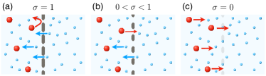
Fig.  4: : Examples of reflection coefficient based on steric exclusion. In (a) the blue solvent only may traverse the pores; while in (b) the red solute particles may also traverse; their permeability through the pores is however small since the accessible volume in the pore for the red solute particles is smaller than that for the blue solvent. (c) The membrane is now fully permeable to all species, and therefore diffusion dominates and solute particles move towards the low concentration side.

Interestingly, cases with negative reflection coefficient, $\sigma<0$, were reported. This situation is often termed anomalous osmosis ^{40, 41} and it corresponds to situations where the solute is more permeable than the solvent. We will discuss in Sec. 4 various examples where such a situation with reversed osmosis occurs.

The specificity of the membrane and its interaction with the solute molecules actually come into play into this reflection coefficient $\sigma$. A number of models have tried to rationalize the dependence of $\sigma$ on the chemical and physical properties of the components. The first models took into account steric effects (similar to Fig. 4), where in fact the volume accessible to the solute inside the pore would differ (because of its typically larger size) than that accessible to the solvent ^{42, 43, 44}. The next generation of models sought to include as well hydrodynamic interactions, investigating how friction induced by the proximity of the solute to the pore walls would reduce permeability ^{45, 46}. Anderson also studied interactions with the pore walls and adsorption of the solute in the pore ³⁸. Similarly, the “mobility” coefficient $\omega_{s}$ entering the transport equations will depend both on the solute-membrane interactions and transport parameters. A first, naive, estimate is to identify this coefficient with the partition coefficient of the solute between the membrane and the reservoirs at equilibrium, $K_{s}=c_{s}^{\rm m}/c_{s}^{\rm bulk}$, so that $\omega_{s}=K_{s}$ ³¹. But this estimate does not account for the complex transport processes occurring within the membrane. Interestingly, the non-dimensional coefficients $\omega_{s}$ and $\sigma$ are expected to be linearly related, ³¹ as $1-\sigma\propto\omega_{s}$, a result that we will recover below in a specific case.

Altogether, a complete determination of the reflection and mobility coefficients requires to implement a microscopic description of the membrane-fluid interactions. We will explore below and in Sec. 3 various situations highlighting how playing with interactions may lead to advanced osmotic transport behavior.

2.4 Mechanical views of osmosis: a tutorial perspective

Beyond the general formalism introduced above, it is interesting to get further fundamental insights into the microscopic mechanisms which underlie osmosis. In particular it is of interest to get some intuition on the mechanical force balance associated with the osmotic pressure. To do so, we will reduce the microscopic ingredients of osmosis to their minimal function and this description has merely a tutorial purpose. Still it is very enlightening in order to understand how the connection between “microscopic” parameters and thermodynamic forces builds up. Such mechanistic views of osmosis also allow to envision advanced osmotic phenomena, beyond the van ’t Hoff perspective. Alternative approaches with similar illustrative objectives were proposed for one-dimensional single file channels, see Refs.47, 48.

We pointed out above that the van ’t Hoff law for the osmotic pressure does not involve the membrane properties per se, provided that it is semi-permeable. So it is tempting to replace the membrane by a crude equivalent, namely an energy barrier acting on the solute only, say $\mathcal{U}(x)$ (assuming for simplicity a unidimensional geometry) – see Fig. 5. This approach, which captures the minimal ingredients at play in osmosis, was first introduced by Manning ⁴⁹ in the low concentration regime, and generalized more recently to explore the osmotic transport across perm-selective charged nanochannels ⁵⁰ or in non-linear regimes at high solute concentrations ⁵¹. One may note that such a potential barrier can also be physically achieved; for example, it may be generated from a nonuniform electric field acting on a polar solute in a nonpolar solvent ⁵², or it can represent the nonequivalent interactions of solute and of solvent particles with a permeable membrane, e.g., charge interactions ^{53, 50}.

Let us first consider the ideal case where the barrier’s maximum is high, i.e. $\mathcal{U}_{\rm max}\gg k_{B}T$, so that the solute cannot cross the barrier: this is the perfectly semi-permeable case. In both reservoirs the solute is at equilibrium and the solute profile follows accordingly the Boltzmann relation

$$c_{s}^{(r)/(l)}(x)=c_{s}^{(r)/(l)}\times e^{-{\mathcal{U}(x)\over k_{B}T}}$$ (17)

Now, a key remark is that the force on a fluid element of volume $d\tau$ (consisting of the solvent and solute mixture) will write

$$df(x)=c_{s}^{(r)/(l)}(x)\times(-\partial_{x}\mathcal{U}(x))d\tau.$$ (18)

with $d\tau=\mathcal{A}dx$; $\mathcal{A}$ is the membrane area. The total force per unit area acting on the fluid is accordingly integrated over $x$

$${F_{T}\over{\cal A}}=\int_{0}^{\infty}dx\,c_{s}^{(r)}e^{-{\mathcal{U}(x)\over k_{B}T}}\times(-\partial_{x}\mathcal{U}(x))+\int_{-\infty}^{0}dx\,c_{s}^{(l)}e^{-{\mathcal{U}(x)\over k_{B}T}}\times(-\partial_{x}\mathcal{U}(x))$$ (19)

(where we arbitrarily put $x=0$ at the position of the maximum of the energy barrier), leading immediately to

$${F_{T}\over{\cal A}}=k_{B}T\times[c_{s}^{(r)}-c_{s}^{(l)}]\equiv\Delta\Pi$$ (20)

where we neglected terms behaving as $\exp[-\mathcal{U}_{\rm max}/k_{B}T]$. Altogether this simple approach allows one to retrieve the van ’t Hoff law. It highlights the mechanical origin of osmosis: as is transparent from the previous derivation, the osmotic pressure results from the fact that the reservoir containing more solute particle will generate a higher repelling force on the fluid than from the other reservoir: accordingly a fluid flow will be generated from the low to the high concentrations, hence diluting the more concentrated reservoir.

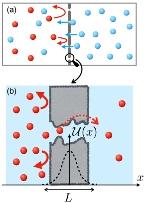
Fig.  5: : The physical force driving osmosis is interaction of the solute with the membrane. (a) The membrane exerts a repulsive force (red arrows) on the solute particles (red) that creates a pressure gradient (or a void on the immediate left hand side of the membrane) that drives the flow (blue arrows of blue solvent particles). (b) Mechanical view of osmosis: the partially permeable membrane may be viewed as an energy barrier for the solute molecules (in red) that they have to overcome in order to traverse the membrane.

While the above approach is instrinsically at equilibrium, it can be easily generalized to a non-equilibrium situation by releasing the assumption of an (infinitely) high energy barrier: in this case the solute can cross the “membrane” between the two reservoirs at a finite rate, see Fig. 5, generating a solute flux. We further assume that the membrane is fully permeable to the solvent (no energy barrier acting on it), with a permeance $\mathcal{L}_{\text{hyd}}$ relating the fluid flux $Q$ to the pressure drop $\Delta p$ in the absence of a concentration difference: $Q=\mathcal{L}_{\text{hyd}}(-\Delta p)$.

The stationary dynamics of the system is described by the coupled set of equations for the solute diffusive dynamics – Smoluchowski equation – and fluid transport – Navier-Stokes equation. In the 1D geometry described above, the stationary solute concentration $c_{s}(x)$ obeys a Smoluchowski equation:

$$0={\partial_{t}}c_{s}= -\partial_{x}j_{s}$$

$$= -\partial_{x}\left(-D_{s}\partial_{x}c_{s}+\lambda_{s}c_{s}\,(-\partial_{x}\mathcal{U})+v_{x}c_{s}\right),$$ (21)

where $j_{s}=J_{s}/\mathcal{A}$ is the solute flux per unit surface, $D_{s}$ is the solute diffusion coefficient, $\lambda_{s}=D_{s}/k_{B}T$ the mobility and $v_{x}$ the local fluid velocity. We will further assume a low Péclet number, $\mathrm{Pe}=v_{x}L/D_{s}\ll 1$, such that the convective term of Eq. (21) is negligible. This is valid for low permeability (nanoporous) membranes. The full derivation including the convective term was considered in Ref.49. Since the solute flux across the membrane $J_{s}$ is constant in time and spatially uniform, Eq. (21) is explicitly solved with respect to the concentration as:

$$c_{s}(x)=c_{s}^{(r)}-\Delta c_{s}\,e^{-\beta\mathcal{U}(x)}{\int_{x}^{L/2}dx^{\prime}\,\exp[+\beta\mathcal{U}(x^{\prime})]\over\int_{-L/2}^{L/2}dx^{\prime}\,\exp[+\beta\mathcal{U}(x^{\prime})]},$$ (22)

where $\beta=1/k_{B}T$. The solute concentration difference between the two volumes is $\Delta c_{s}=c_{s}^{(r)}-c_{s}^{(l)}$. For simplicity we assumed that the barrier has an extension $L$.

Now turning to the momentum conservation equation for the fluid (solvent + solute), the flow field $\bm{v}$ of the fluid obeys a Stokes equation (neglecting inertial terms)

$$0=-\bm{\nabla}p+\eta\bm{\nabla}^{2}\bm{v}+\bm{f}_{ext},$$ (23)

where $p$ is the fluid pressure and $\bm{f}_{ext}$ represents the total volume forces acting on the system, $e.g.$ the forces acting on the solvent and on the solute, here

$$\bm{f}_{ext}=c_{s}(-\bm{\nabla}\mathcal{U}).$$ (24)

The driving force inducing the solvent flow along the $x$ axis is accordingly written in terms of an apparent pressure drop, $-\partial_{x}\mathcal{P}=-\partial_{x}p+c_{s}(x)(-\partial_{x}\mathcal{U})$. The membrane, via its potential $\mathcal{U}$, will therefore create an average force on the fluid, which writes per unit surface

$$-\Delta\mathcal{P}=-\Delta p+\int_{-L/2}^{L/2}dx\,c_{s}\,(-\partial_{x}\mathcal{U})\equiv-\Delta p+\sigma\Delta\Pi,$$ (25)

where $\Delta$ means the difference of a quantity between the two sides. The second term of Eq. (25) can be interpreted as the osmotic contribution. Using the expression for the concentration profile given in Eq. (22), one recovers the classical van ’t Hoff law of the osmotic pressure, $\Delta\Pi=k_{B}T\Delta c_{s}$, and furthermore obtains an expression for the reflection coefficient $\sigma$ as

$$\sigma=1-{L\over\int_{-L/2}^{L/2}dx^{\prime}\,\exp[+\beta\mathcal{U}(x^{\prime})]}.$$ (26)

The above result correctly recovers the case of a completely semi-permeable membrane (no solute flux across the membrane), i.e., $\beta\mathcal{U}\gg 1$ and $\sigma\rightarrow 1$, yielding $-\Delta\mathcal{P}=-\Delta[p-\Pi]$. In the intermediate cases, although the membrane is permeable, a flow arises due to the solute concentration gradient even in the absence of an imposed pressure gradient. When the potential is repulsive and small $\mathcal{U}\sim k_{B}T$, then $0<\sigma<1$; the flow is in the direction of increasing concentration.

Integrating Eq. (23) over the membrane area ($\mathcal{A}$) and thickness ($L$) allows the total flux $Q$ to be expressed as

$$Q=-\mathcal{L}_{\text{hyd}}\left(\Delta p-\sigma k_{B}T\Delta c_{s}\right).$$ (27)

Here the permeance $\mathcal{L}_{\rm hyd}$ can be expressed in terms of the permeability, $\kappa_{\rm hyd}$, as $\mathcal{L}_{\text{hyd}}={\mathcal{A}\over L}{\kappa_{\rm hyd}\over\eta}$. The permeability $\kappa_{\rm hyd}$ is defined formally in terms of the flow as $\kappa_{\rm hyd}^{-1}=\langle-\nabla^{2}v\rangle/\langle v\rangle$, where $\langle\cdot\rangle=\mathcal{V}^{-1}\int\int dx\,d\mathcal{A}\,(\cdot)$ denotes an average over the pore volume, here $\mathcal{V}=\mathcal{A}\,L$. These parameters, $\kappa_{\rm hyd}$ and $\mathcal{L}_{\text{hyd}}$, take into account the detailed geometry of the pores in the membrane (pore cross section, length, etc.). Overall Eq. (27) agrees with the Kedem–Kachalsky result in Eq. (15). While this approach is derived here in the dilute regime for the solute, it can be generalized to arbitrary concentrations, see Ref.51.

As a last remark, it is interesting to note that the mechanistic approach highlights an underlying fundamental symmetry in the transport phenomenon. Indeed Eq. (25) introduces the osmotic pressure as the driving force on the fluid: $\int_{-L/2}^{L/2}dx\,c_{s}\,(-\partial_{x}\mathcal{U})=\sigma\Delta\Pi$. Now the Smoluchowski equation for the solute – integrated over the membrane thickness $L$, Eq. (21) – contains the very same term and one may accordingly rewrite the solute flux as

$$J_{s}=-{D_{s}\over L}\mathcal{A}\left[\Delta c_{s}-\sigma{\Delta\Pi\over k_{B}T}\right]$$ (28)

The solute flux is therefore intimately related to the osmotic pressure. As is transparent from this equation, the van ’t Hoff osmotic pressure is fully expressed, i.e. $\Delta\Pi=k_{B}T\Delta c_{s}$, only when the solute flux vanishes $J_{s}=0$ ($\sigma=1$ and $\omega_{s}=0$). Reversely for a fully permeable membrane $J_{s}=-{D_{s}\mathcal{A}\over L}\Delta c_{s}$, and there is no osmotic pressure ($\sigma=0$ and $\omega_{s}=1$). Finally this equation can be rewritten as $J_{s}=-D_{s}\mathcal{A}(1-\sigma)\Delta c_{s}/L$, so that the “mobility” coefficient $\omega_{s}$ is related here to the reflection coefficient as $\omega_{s}=1-\sigma$.

In this first part we have reviewed the basic understanding of osmosis, from the historical discovery of the phenomenon to the precise understanding of the effect in terms of thermodynamic forces. Although simplistic, the previous mechanical/kinetic approach provides a fruitful and complementary perspective on osmotic transport, which suggests a number of generalizations – that we will discuss below. It also reveals that the key aspect of osmosis is not really the membrane itself, but the existence of differential forces acting separately on the solvent and the solute. This is crucial to understand a number of phenomena related to osmosis that we discuss below.

3 Osmosis without a membrane

Situations where differential forces act on the solvent and the solute occur naturally, especially at interfaces: for example a charged surface does act specifically on dissolved ions, repelling co-ions and attracting counter-ions; or a neutral hard wall will repel polymers via excluded volume. As we now discuss in the following sections, these specific forces may be harnessed to induce interfacially-driven osmotic flows.

The geometry we will consider here involves a solid surface along which a solute gradient, or more generally a thermodynamic force – an electric field, a temperature gradient… – is established, as sketched in Figs. 6-7. Under an electric field, the net electric forces occurring within the diffuse interface close to the solid will push the fluid and generate a so-called electro-osmosis flow for the solvent. But as we will show below, a solute gradient $\nabla c_{\infty}$ parallel to the surface can also generate fluid motion whose amplitude is proportional to $\nabla c_{\infty}$:

$$v_{DO}\propto\nabla c_{\infty}.$$ (29)

This latter phenomenon is usually coined as diffusio-osmosis. The phenomenon bears some fundamental analogy with Marangoni effects where a gradient of surface tension at an interface may drive fluid (or reversely particle) motion as $v_{f}\propto\nabla\gamma_{LV}$ ⁵⁴. Now extending Marangoni flows to solid-fluid interfaces is definitely not obvious, but it was recognized by Derjaguin and collaborators ^{55, 56} that the diffuse nature of the interface may allow the fluid to “slip” over the solid surface under a concentration gradient. Diffusio-osmosis is accordingly an interfacially driven flow, and takes its origin in the interfacial structure of the solute close to the solid surface, within the first few nanometers close to the surface.

3.1 From electro- to diffusio- osmosis

3.1.1 From electro-osmosis…

Let us start with the canonical example of electro-osmosis, i.e. the fluid flow close to a solid surface generated under an applied electric field. A solution containing ions will build up a so-called electric double layer (EDL) close to any charged surface: counter-ions are attracted by the surface charge, while co-ions are repelled. The surface charge, say $\Sigma$, is balanced in the fluid by a density of charge $\rho_{e}=e(c_{+}-c_{-})$, defined as the difference between the density of positive and negative ions (assuming monovalent ions here for illustrative purposes). The resulting double layer is diffuse and extends over a finite width, see Fig. 6. The structure of the EDL was amply discussed in many textbooks and reviews, and we refer in particular to Refs.57, 58, 59 for further insights. As a rule of thumb, the extension of the EDL is typically given by the Debye screening length ^{58, 60}, defined as

$$\lambda_{D}={1\over\sqrt{8\pi\ell_{B}c_{s}}}$$ (30)

where $c_{s}$ is the (bulk) salt concentration in the bulk and $\ell_{B}=e^{2}/4\pi\epsilon k_{B}T$ is the Bjerrum length ($\epsilon$ is the dielectric permittivity of water). Typically for water at room temperature, $\ell_{B}=0.7$nm and the Debye length ranges between 30nm for a salt concentration of $10^{-4}$mol.l^-1 to 0.3nm for a 1mol.l^-1 salt concentration.

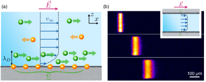
Fig.  6: : Electro-osmosis. (a) In the presence of a surface charge $\Sigma$, an electrical double layer forms extending typically over a distance fixed by the Debye length $\lambda_{D}$. Under an applied electric field $\vec{E}$ parallel to the surface, a net electric force builds up due to the unbalanced charge within the electric double layer. It drives a solvent flow parallel to the surface, extending as a flat flow profile into the bulk. (b) Visualization of the electro-osmotic flow in a capillary, via the displacement of (neutral) tagged molecules. In contrast to the parabolic Poiseuille flow, the electro-osmotic flow profile takes the form of a plug flow, which barely disperses the dye. Reproduced from Ref.61 with permission from Springer Nature, copyright 2005.

Within the EDL, there is a net charge density in the fluid, and whenever an external electric field is applied to the fluid (parallel to the surface), this will generate a net bulk force $\rho_{e}E$. The Stokes equation for the fluid velocity writes accordingly in the direction $x$ (parallel to the solid interface)

$$\eta\partial_{zz}v+\rho_{e}E=0$$ (31)

where $z$ is the direction perpendicular to the interface. The pressure-gradient term vanishes for the shear-flow considered here. Using the Poisson equation $\rho_{e}=-\epsilon\partial_{zz}V_{e}$, relating the charge density to the electric potential $V_{e}$ in the fluid, one can integrate twice Eq. (31) to obtain the velocity profile

$$v(z)=-\frac{\epsilon E}{\eta}\left[V_{e}(z=0)-V_{e}(z)\right]$$ (32)

where a no-slip boundary condition was assumed here. The electrical potential at the interface is usually identified as the zeta potential $V_{e}(z=0)=\zeta$. The electro-osmotic velocity is constant beyond the EDL and reaches its asymptotic value

$$v_{\infty}=\mu_{EO}E$$ (33)

where $\mu_{EO}=-\frac{\epsilon\,\zeta}{\eta}$ is the electro-osmotic mobility. In the presence of hydrodynamic slippage on the surface, the electro-osmotic mobility is typically enhanced by a factor $1+b/\lambda_{D}$, where $b$ is the slip length, see Refs.62, 63, 64 for more details. We finally note that the $\zeta$-potential may be rewritten as a function of the electrical concentration $\rho_{e}$ (by integrating twice Eq. (31))

$$\zeta=-\frac{1}{\epsilon}\int_{0}^{\infty}z\,\rho_{e}(z)dz.$$ (34)

From a physical point of view, electro-osmosis may be seen as a force balance between the viscous friction force at the interface and the electrostatic driving force within the EDL. The velocity field is expected to establish over the Debye length $\lambda_{D}$ and thus the fluid friction force is typically $\sim\eta v_{\infty}/\lambda_{D}$. Now the body electrical force within the EDL is simply $\Sigma\times E$ where $\Sigma$ is the surface charge. From Gauss’ electrostatic boundary condition, we have $\Sigma=-\epsilon\partial_{z}V_{e}|_{z=0}\approx-\epsilon\zeta/\lambda_{D}$. Altogether the force balance thus takes the form

$$\eta{v_{\infty}\over\lambda_{D}}\approx\Sigma\times E\approx-{\epsilon\zeta\over\lambda_{D}}\times E$$ (35)

and this leads accordingly to the expression in Eq. (33) for the electro-osmotic mobility. A simple extension of this argument highlights immediately the potential role of hydrodynamic slippage: with a slip length $b$, the viscous friction force will reduce to $\sim\eta v_{\infty}/(\lambda_{D}+b)$ while keeping the body force identical, so that the electro-osmotic velocity will be increased by a factor $1+b/\lambda_{D}$. Altogether, the electro-osmotic flow thus takes its origin within the very few nanometers close to the boundary and can be therefore strongly affected by molecular details: hydrodynamic slippage ⁶², nanoscale roughness ⁶⁵, contamination ⁶⁶, dielectric inhomogeneities ⁶⁷, etc. This makes the underlying physics of interfacial transport both complex and very rich.

3.1.2 … To diffusio-osmosis …

While electro-osmosis corresponds to interfacially driven fluid motion under an external electric field, diffusio-osmotic motion occurs under the gradient of a solute, $\partial_{x}c_{\infty}$, in the vicinity of a solid surface – see Fig. 7. Similarly to electro-osmosis, a key ingredient is the specific interaction of the solute with the surface, which occurs within a diffuse layer of finite thickness. Reflecting the discussion of osmosis across a model potential barrier in Sec. 2.4, the solute will be assumed to interact via an external potential $\mathcal{U}(z)$ with the solid surface. One noticeable difference to the previous membrane case though is that this potential now acts perpendicular to the solid surface and solute gradient (i.e. depending on $z$ but not on $x$), see Fig.7.

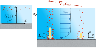
Fig.  7: : Diffusio-osmosis. A gradient of solute imposed far from the surface induces a fluid flow. Here the solute is assumed to interact with the surface via an interaction potential $\mathcal{U}(z)$ (an adsorbing profile on the figure). The solute interaction with the surface induces a force on the fluid, here towards the surface, which is higher in the more concentrated area. This normal force converts into a parallel pressure drop which generates a fluid flow from high to low concentrations (and reversely for a repelling interaction).

Diffusio-osmosis with neutral solutes – We first consider the case of neutral solutes. The fluid velocity and solute density obey the coupled Stokes and Smoluchowski equations, which write in the stationary state as:

$$0= -\bm{\nabla}p+\eta\bm{\nabla}^{2}\bm{v}+(-\bm{\nabla}\mathcal{U}),$$ (36)

$$0= -\bm{\nabla}\cdot\left[-D_{s}\bm{\nabla}c_{s}+\lambda_{s}c_{s}\,(-\bm{\nabla}\mathcal{U})+\bm{v}c_{s}\right]$$

At infinity, we assume a fixed gradient $\partial_{x}c_{\infty}$ along $x$ for the solute concentration.

These coupled equations are strongly entangled. However in the limit of a thin interfacial layer – corresponding to a range for the potential $\mathcal{U}(z)$ which is small compared to the lateral variations of the solute gradient –, one expects the concentration profile to relax quickly to a local equilibrium across the diffuse layer $c_{s}(x,z)\simeq c_{\infty}(x)\exp(-\mathcal{U}(z)/k_{B}T)$.

Turning now to the fluid transport equation, the Stokes equation projected along the $z$ direction writes simply

$$0=-\partial_{z}p+c_{s}(-\partial_{z}{\cal U})$$ (37)

because the $z$ component of fluid velocity is expected to be negligible for thin layers. We can integrate this pressure balance to obtain

$$p(x,z)-p_{\infty}=k_{B}Tc_{s}(x,z)-k_{B}Tc_{\infty}(x)$$ (38)

which can be seen as an osmotic equilibrium across the diffuse layer ⁶⁸. In simple terms, the existence of a specific solute-wall interaction allows the membrane to “express” the solute osmotic pressure $\Pi(x,z)=k_{B}Tc_{s}(x,z)$ within the interfacial layer. However the effects of the latter disappear in the bulk ($z\rightarrow\infty$) and there is no bulk osmotic pressure gradient.

Now inserting the pressure from Eq. (38) into the Stokes equation projected along $x$, see Eq. (36), leads to

$$\eta\partial_{z}^{2}v_{x}-\partial_{x}[p(x,z)-p_{\infty}]=0.$$ (39)

Following the same steps as for the electro-osmosis, one obtains the fluid velocity along the $x$ coordinate in the bulk fluid as

$$v_{\infty}=\mu_{DO}\times(-k_{B}T\nabla_{x}c_{\infty})$$ (40)

with the diffusio-osmotic mobility $\mu_{DO}$ given by

$$\mu_{DO}=\frac{1}{\eta}\int_{0}^{\infty}\,z\,\left(\frac{c_{s}(x,z)}{c_{\infty}}-1\right)dz=\frac{1}{\eta}\int_{0}^{\infty}\,z\,\left(\exp\left(\frac{-\mathcal{U}(z)}{k_{B}T}\right)-1\right)dz.$$ (41)

This expression is similar to Eq. (34) for the electro-osmotic mobility. The effect of hydrodynamic slippage on the surface can also be taken into account, along the same lines as in Refs.69, 70 and leads to an enhancement factor of the diffusio-osmotic mobility scaling as $(1+b/\lambda)$, where $b$ is the slip length and $\lambda$ is the typical width of the diffuse interface. The amplification effect is expected to be massive on superhydrophobic surfaces ⁷⁰ and amplification by orders of magnitude are predicted. Interestingly for strongly hydrophobic surfaces where the liquid-vapor interface dominates, the diffusio-osmotic velocity takes the physically transparent expression $v_{DO}={b_{\rm eff}\over\eta}\nabla\gamma_{LV}$, where $b_{\rm eff}$ is the effective slip length on the superhydrophobic surface and $\gamma_{LV}$ is the (solute concentration dependent) surface tension of the liquid-vapor interface.

Similarly as in electro-osmosis, diffusio-osmosis can be interpreted in terms of a simple force balance within the diffuse layer. A first integration of Eq. (39) indeed shows that diffusio-osmotic flow results from the balance between the viscous stress on the surface and an osmotic pressure gradient integrated over the diffuse layer:

$$0=\eta\partial_{x}v_{x}|_{wall}+\int_{0}^{\infty}dz\,\partial_{x}\left[\Pi(x,z)-\Pi_{\infty}(x)\right]$$ (42)

Simple estimates of the various terms lead to a more qualitative version of this force balance as

$$\eta\frac{v_{\infty}}{\lambda}\sim\pm\lambda\times(-k_{B}T\nabla_{x}c_{\infty})$$ (43)

where $\lambda$ is defined here as the range of the potential $\cal U$, and the $\pm$ sign depends on whether the solute is attracted or depleted by the surface. This leads to $v_{\infty}\sim\pm{\lambda^{2}\over\eta}\times(-k_{B}T\nabla_{x}c_{\infty})$ in full agreement with Eqs. (40)-(41).

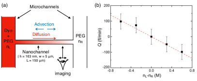
Fig.  8: : Experimental evidence for diffusio-osmosis. (a) A gradient of polyethylene glycol polymer PEG is maintained along a nanochannel thanks to lateral microchannels acting as reservoirs. The nanochannel is 160nm in thickness and is fully permeable to PEG. Under a PEG concentration gradient, a diffusio-osmotic flow arises: water moves towards higher concentrations of PEG. The flow rate $Q$ is measured via the concentration profile of a dye. (b) Measured diffusio-osmotic flux $Q$ as a function of the PEG concentration difference, showing a velocity proportional to the PEG concentration difference. This behavior and the sign of the effect are consistent with a steric exclusion of PEG on the surfaces, as predicted in Eq.(44). (a) and (b) are reproduced and adapted from Ref.25 with permission from the American Physical Society (APS), copyright 2014.

Diffusio-osmosis is definitely an osmotic flow, e.g. a flow driven by an osmotic pressure gradient located within the diffuse layer. However the direction of the diffusio-osmotic flow can be along or against the gradient of the solute, in strong contrast to bare osmosis which induces a flow towards the highest solute concentration. That is highlighted in the expression of the diffusio-osmotic mobility, Eq. (41), which can be positive or negative depending on the attractive or repulsive nature of the interaction potential $\mathcal{U}(z)$. As a rule of thumb, the sign of the mobility will be dominantly determined by the adsorption $\Gamma=\int_{0}^{\infty}dz\left({c(x,z)/c_{\infty}(x)}-1\right)$. If there is a surface excess ($\Gamma>0$ or $\mathcal{U}(z)<0$), the solvent flow goes towards the low concentrated area ($\mu_{DO}>0$). That may appear as surprising because it amounts to concentrating even more the already concentrated solution; we shall discuss this apparent paradox in Sec. 3.2.2. Reversely a surface depletion resulting from a repulsion of the solute from the wall ($\Gamma<0$ or $\mathcal{U}(z)>0$) reverses the direction of the solvent flow towards the high concentrated zone ($\mu_{DO}<0$). An interesting limiting case for this behavior is exemplified by a solute interacting with the wall via steric effect, i.e. hard-core excluded volumes. For a solute particle with radius $R$, the mobility in Eq. (39) reduces to

$$\mu_{DO}^{\rm steric}=-{R^{2}\over 2\eta}.$$ (44)

This behavior was measured in particular in Ref.25 for the diffusio-osmotic flow under a neutral polymer concentration gradient, see Fig. 8 for an illustration. A final remark is that this simple rule for the correlation between adsorption and the sign of diffusio-osmosis is not exact and may fail for more complex interactions between the solute and the wall, for instance with an oscillatory spatial dependence of the concentration profile due to layering. The sign of $\mu_{DO}$ may then be expected to differ from the sign of the adsorption $\Gamma$. In this case, no obvious conclusion can be made for the direction of the diffusio-osmotic velocity and a full calculation has to be made, see for example Ref.26.

Diffusio-osmosis with electrolytes – We now discuss specifically the case of diffusio-osmosis under salinity gradients. Here, as for electro-osmosis, the diffuse layer corresponds to the electric double layer created close to a charged surface, see Fig. 9. The derivation follows similar steps as above, from Eqs. (36) to (41), except that one has to take into account the spatial distribution of both the counter- and co- ions in the EDL that follow a Poisson-Boltzmann distribution, see Ref.71. In this case the diffusio-osmotic velocity is shown to take the form

$$v_{\infty}=D_{DO}(-\nabla\log c_{\infty})$$ (45)

where we introduced a mobility $D_{DO}$ which has now the units of a diffusion coefficient. It takes the expression ⁵⁴

$$D_{DO}={k_{B}T\over 2\pi\eta\ell_{B}}\times\log\left(\cosh^{2}{\Phi_{0}\over 4}\right)$$ (46)

where $\Phi_{0}=eV_{0}/k_{B}T$ is the dimensionless surface potential $V_{0}$ (usually identified with the zeta potential). Note that for an electrolyte with unequal diffusion coefficients for the anions and cations ($D_{+}\neq D_{-}$), a diffusion electric field builds up under the gradient of the salt concentration (if no current exists in the bulk). This takes the form $E_{\rm diff}={k_{B}T\over e}\delta\nabla\log c_{\infty}$ with $\delta=(D_{+}-D_{-})/(D_{+}+D_{-})$ and adds a supplementary electro-osmotic contribution to the diffusio-osmotic velocity as $v_{\rm diff}=-{\epsilon\zeta\over\eta}\times E_{\rm diff}$. Accordingly this leads to a supplementary contribution to the mobility as:

$$D_{DO}^{\rm diff}=-{\epsilon\zeta\over\eta}\times{k_{B}T\over e}\delta$$ (47)

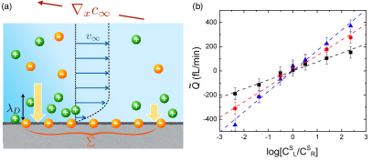
Fig.  9: : Diffusio-osmosis with charged electrolytes. (a) Geometry; an electrolyte concentration difference is imposed far from the charged interface. The electrical interaction with the surface induces an (attractive) electrostatic force – sketched with arrows– on the fluid which is larger where the salt concentration is larger, hereby inducing a net flow towards the low salinity region. (b) Measurement of the diffusio-osmotic flux as a function of the difference of the logarithm of the salt concentration between two reservoirs, in a similar way as in Fig. 8. Note the reversal of the sign as compared to Fig. 8-b. Reproduced from Ref.25 with permission from the APS, copyright 2014

An important remark is that for electrolytes the velocity is proportional to the gradient of the logarithm of salt concentration, in contrast to solutes where it is basically linear in the gradient, see Eq. (40). We will refer to this dependence as “log-sensing” by analogy to behaviors occurring for the chemotaxis of biological entities (e.g. bacteria). Such a dependence may be understood on the basis of the simple scaling argument based on the force balance above, see Eq. (43). Indeed the thickness of the diffuse layer is now given by the Debye length, and $v_{\infty}\simeq{\lambda_{D}^{2}\over\eta}\times(-k_{B}T\nabla_{x}c_{\infty})$. Since the Debye length depends on the salt concentration as $\lambda_{D}^{2}=(8\pi l_{B}c_{\infty})^{-1}$, one obtains :

$$v_{\infty}\approx-\frac{k_{B}T}{8\pi\eta l_{B}}\nabla_{x}\log c_{\infty}.$$ (48)

which is qualitatively similar to the exact results in Eq. (46) and predicts log-sensing for diffusio-osmosis with electrolytes.

This behavior is confirmed by experimental investigations of water flows under salinity gradients in nanofluidic circuits ²⁵, see Fig. 9. Diffusio-osmotic flow of water under salinity gradients was also evidenced across carbon nanotube membranes⁷², confirming further that diffusio-osmosis was acting against bare osmosis. In an alternative configuration, diffusio-osmosis was also shown to induce very large ionic currents under salinity gradients ^{73, 74, 75}. We will come back to such cross effects associated with diffusio-osmosis in Sec. 3.2.1, as well as in the section dedicated to blue energy harvesting, Sec. 6.3. In a very different field, diffusio-osmotic flows were also shown to strongly impact and shape the reactive fluid flows occurring in the solid Earth ⁷⁶. Log-sensing has also many counter-intuitive consequences and a variety of applications ^{77, 78}, which we will discuss more specifically in the context of diffusio-phoresis in Sec. 5.

Solvo-osmosis and diffusio-osmosis with mixtures – Up to now we considered merely dilute solute solutions, but all previous results can be generalized to mixtures of liquids with any molar fraction of its constituents. The key ingredient remains that the two constituents interact differently with the solid substrate. As shown in Ref.51, the diffusio-osmotic velocity now takes the expression

$$v_{\infty}=\mu_{DO}(-\nabla_{x}\Pi[X_{\infty}(x)]),$$ (49)

where $\Pi$ is the generalized osmotic pressure defined in Eq. (9), calculated for the molar fraction $X_{\infty}$, hence generalizing the expression in Eq. (40). The diffusio-osmotic mobility $\mu_{DO}$ is still given by the initial expression $\mu_{DO}=\frac{1}{\eta}\int_{0}^{\infty}dz^{\prime}\,z^{\prime}\,\left({c_{s}(x,z^{\prime})\over c_{\infty}(x)}-1\right)$. However, for a solute-substrate interaction potential ${\cal U}$, the concentration profile $c_{s}(x,z)$ is now implicitly related to the value in the bulk $c_{\infty}(x)$ via the local equilibrium condition $\mu[c_{s}(x,z)]+{\cal U}(z)\simeq\mu[c_{\infty}(x)]$.

Diffusio-osmosis with ethanol-water mixtures was investigated recently in Ref.26. But the majority of existing experimental investigations merely explored the reverse configuration of phoretic transport of particles under gradients of liquid composition, denoted as “solvo-phoresis” ^{79, 21}. Interestingly in Ref.21, the phoretic transport of colloidal (polystyrene) particles in ethanol-water mixtures resulted in a “log-sensing” behavior of the particle diffusio-phoretic velocity, obeying $V=D_{SP}\nabla\log X$, with here $X$ the ethanol mole fraction.

3.1.3 … And electro-chemical equivalence.

In the case of electrolytes, the two previous transport phenomena, electro- and diffusio- osmosis, are fundamentally intertwined. Indeed, from the thermodynamic point of view, the chemical potential and the electric potential contributions merge into the electrochemical potential: $\mu_{\rm el}=\mu+qV$ (with $q$ the ion charge and $V$ the electric potential). There is accordingly a deep analogy when driving the system under gradients of chemical potential (diffusio-osmosis) or driving under gradients of electric potential (electro-osmosis). An illuminating discussion on this point and the corresponding force balance is provided by T. Squires in Ref.59, 80 and we reproduce the essentials of the argumentation here.

Let us consider in full generality that a gradient of the electrochemical potential is applied in the bulk far from the boundary, $\nabla\mu_{\rm el,i}^{B}$ (along the direction of the solid surface, say $x$); the index $i$ runs over the various ion species in the solution. As we discussed above for both electro- and diffusio- osmosis, this will generate net thermodynamic forces on individual ion specie $i$, which may be written as $f_{i}(x,z)=-\nabla\mu_{\rm el,i}(x,z)$. A key remark is that the electrochemical potential is approximately constant across the EDL, i.e. $\mu_{\rm el,i}(x,z)\simeq\mu_{\rm el,i}^{B}(x)$, so that the individual force rewrites $f_{i}(z)\simeq-\nabla\mu_{\rm el,i}^{B}$. The interfacial motion results from the forces in excess to the bulk, so that the corresponding total force acting on the fluid rewrites

$$f_{T}=\sum_{i=1,n}\Delta c_{i}\times f_{i}(z)=\sum_{i=1,n}\Delta c_{i}\times(-\nabla\mu_{\rm el,i}^{B})$$ (50)

where the sum runs over $n$ ion species and $\Delta c_{i}=c_{i}(x,z)-c_{i}^{B}(x)$ is the excess ion concentration in the boundary layer, as compared to the bulk. This driving force will generate a flow according to the Stokes equation $\eta\partial^{2}_{z}v_{x}+f_{T}=0$ and following the same steps as above, one obtains the far field slip velocity as

$$v_{\infty}=-\sum_{i=1,n}{1\over\eta}\nabla\mu_{el,i}^{B}\int_{0}^{\infty}dz\,z\,\Delta c_{i}(z)\equiv\sum_{i}M_{i}(-\nabla\mu_{el,i}^{B}),$$ (51)

where the mobility $M_{i}$ takes the expression $M_{i}={1\over\eta}\int_{0}^{\infty}dz\,z\Delta c_{i}(z)$. For symmetric and monovalent ions, these mobilities can be exactly calculated using Poisson-Boltzmann framework, leading to

$$M_{\pm}={\epsilon\over e\eta}\left[\mp{\zeta\over 2}+{k_{B}T\over e}\times\log\left(\cosh^{2}{\Phi_{0}\over 4}\right)\right]$$ (52)

with $\Phi_{0}=eV_{0}/k_{B}T$ the dimensionless surface potential and here $\zeta\equiv V_{0}$ the zeta potential.

Under a constant electric field $\nabla\mu_{\pm}^{B}=\mp eE_{0}$ and the electro-osmotic mobility is predicted as $\mu_{EO}={1\over e}(M_{+}-M_{-})$, in full agreement with the previous result in Eq. (33)-(34). Under an imposed ionic strength gradient in the bulk, then $\nabla\mu^{B}_{\pm}=k_{B}T\nabla\log c_{\pm}$ are identical and $M_{DO}=M_{+}+M_{-}\equiv D_{DO}$, again in full agreement with the previous result in Eq. (46).

3.2 Transport matrix and symmetry considerations

3.2.1 Transport matrix and cross fluxes

As introduced in Sec.2.3, the framework of irreversible processes allows one to write a linear relation between thermodynamic forces and fluxes ³⁰. Adding the electric forces to the set of forces, one may generalize the results in Eq. (14) to obtain linear transport equations now relating the solvent flux $Q$, excess solute flux $J_{s}-c_{s}Q$ and electric current $I_{e}$ to the pressure gradient $-\nabla p$, chemical potential gradient $-\nabla\mu$ and the applied electric field $-\nabla V_{e}$, and summarized as

$$\left(\begin{array}[]{c}Q\\ {J_{s}-c_{s}Q}\\ I_{e}\end{array}\right)={\mathbb{L}}\times\left(\begin{array}[]{c}-\nabla p\\ -\nabla\mu\\ -\nabla V_{e}\end{array}\right),$$ (53)

Due to Onsager principle, this matrix is symetric and positive definite ³⁰. Each term of this matrix corresponds to a specific transport phenomenon. Diagonal terms are associated respectively with permeability (characterizing solvent flux under a pressure drop), diffusion (characterizing solute flux under an applied solute gradient) and electrical conductance (characterizing ionic current under an applied electric field). The off-diagonal terms correspond to cross effects. We detail below the cross effects that are all recapitulated in Fig. 10.

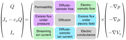
Fig.  10: : Transport Matrix. Explicit transport matrix ${\mathbb{L}}$ as presented in Eq. (53), with colors indicating symmetric terms.

In the first row of the matrix, electro-osmosis and diffusio-osmosis – explored so far – correspond to the terms relating the solvent flux $Q$ to a chemical gradient $-\nabla\mu$ and an electric field $-\nabla V_{e}$ respectively. A key consequence of the symmetry of the matrix is that the same mobilities characterize symmetric transport phenomena. For example consider the first column of the matrix ${\mathbb{L}}$, one finds that the electro-osmotic mobility and diffusio-osmotic mobility also describe respectively the electric current and excess solute flux generated under a pressure drop, as

$$I_{e}={\cal A}\,\mu_{EO}\times(-\nabla p)$$

$$J_{s}-c_{s}Q={\cal A}\,\mu_{DO}\times(-\nabla p)$$ (54)

where ${\cal A}$ is the channel cross section. The first corresponds to the so-called streaming current and takes its origin in the motion of mobile ions in the EDL which are carried by the pressure-driven flow; the pressure-driven excess solute flux has a similar physical origin.

Streaming currents are commonly measured in experiments ^{60, 62}, even down to single carbon and boron-nitride nanotubes ⁷³. To our knowledge, no experimental measurement of pressure-driven excess solute flux has been performed up to now. However this is not the case in molecular dynamics simulations where it is far easier to measure the diffusio-osmotic mobility via the pressure-driven excess flux ^{69, 26}– see details in Sec. 3.5.

Now, the transport matrix suggests that an electric current can be generated under an osmotic gradient, which we term here the diffusio-osmotic ion current, following

$$I_{DO}=K_{\rm osm}\times(-\nabla\log c_{\infty}).$$ (55)

Let us consider a channel in the form of a slit of width $w$ and height $h$ (with $w\gg h$ to simplify). Using Poisson-Boltzmann to describe the EDL, one can calculate the corresponding osmotic electric current ^{81, 73, 64} and the mobility takes the form

$$K_{\rm osm}=\alpha\,\times(-\Sigma){k_{B}T\over 2\pi\eta\,\ell_{B}}\left(1-{\sinh^{-1}\chi\over\chi}\right)$$ (56)

where $\alpha\simeq 2w$ is the perimeter of the channel cross section. In this expression we introduced $\chi=\sinh{|\Phi_{0}|\over 2}$ with $\Phi_{0}=eV_{0}/k_{B}T$ the dimensionless surface potential $V_{0}$. In the Poisson-Boltzmann framework $\chi$ is related to the surface charge $\Sigma$ according to $\chi=2\pi\ell_{B}\lambda_{D}|\Sigma|/e$ with $\lambda_{D}$ the Debye length, so that $\chi\propto|\Sigma|$. This formula can be extended to take slippage on the surface into account, as well as mobile surface charges ⁶⁴. More precisely the diffusio-osmotic ion current takes its origin in the motion of ions in the EDL which are carried by the diffusio-osmotic flow. As a simple estimate we may write that $I_{DO}\approx(-\Sigma)\times v_{DO}$, where $v_{DO}$ is the diffusio-osmotic velocity: using the expression Eq. (40) for $v_{DO}$, one indeed recovers Eq. (56). However the prediction of Eq. (56) reports a more complex dependence, since the linear dependence in $\Sigma$ is only valid for large enough $\Sigma$, while for low $\Sigma$, one finds that $K_{\rm osm}\propto\Sigma^{3}$, i.e. vanishingly small. Such osmotically driven currents have been measured experimentally in various systems, nanochannels, single nanotubes, single nanopores – see Refs.82, 73, 74, 83 – to cite a few. This effect finds important applications in the context of blue energy harvesting⁷⁵, that we will explore in detail in Sec. 6.3.

3.2.2 Entropy production with diffusio-osmosis

We pointed out above that the sign of the diffusio-osmostic mobility, $\mu_{DO}$, can be either positive or negative, so that the corresponding flux can be along or against the concentration gradient. A negative $\mu_{DO}$ may appear at first sight striking since the direction of the solvent flow corresponds to that of an increase in salt concentration, thus leading to an apparent violation of the second principle. This is however not the case, as it can be verified from a calculation taking into account all relevant fluxes. To highlight this situation, let us consider a membrane separating two reservoirs with fixed volumes; the concentration on the left/right reservoir is $c_{s}(t)=c_{0}\mp{\Delta c_{s}(t)\over 2}$. The pore size is assumed here to be larger than the solute diameter so that the membrane is permeable to the solute and there is no bare osmotic pressure. A salinity gradient however generates a diffusio-osmotic flow on the pore surface. Based on the transport matrix formulation, Eq. (14), one may write the solvent and (excess) solute fluxes as a function of the solute concentration and pressure gradients according to:

$$Q ={{\cal A}_{p}\over L}\left[\kappa(-\Delta p)+\mu_{DO}(-k_{B}T\Delta c_{s})\right]$$ (57)

$$J_{s}-c_{0}Q ={{\cal A}_{p}\over L}\left[\mu_{DO}\,c_{0}(-\Delta p)+\lambda_{s}(-k_{B}T\Delta c_{s})\right]$$

with ${\cal A}_{p}$ the total (open) pore area of the membrane, $L$ its thickness and $\lambda_{s}=D_{s}/k_{B}T$ the diffusive mobility of the solute across the membrane, defined in terms of the solute diffusion coefficient; $\kappa$ is defined in terms of the permeance as $\mathcal{L}_{\rm hyd}\equiv\kappa{{\cal A}_{p}/L}$ (note that $\kappa=\kappa_{\rm hyd}/\eta$ where $\kappa_{\rm hyd}$ is the permeability introduced above). The second principle imposes that the transport matrix in Eqs. (14) & (57) should be definite positive. Accordingly, the determinant $\det(\mathbb{L})\propto\kappa\lambda_{s}-\mu_{DO}^{2}c_{0}$ must be strictly positive.

On the other hand, since the volume is fixed, the flux vanishes, $Q=0$, and the solute flux writes

$$J_{s}={{\cal A}_{p}\over L}{1\over\kappa}\left[\lambda_{s}\,\kappa-{\mu_{DO}^{2}\,c_{0}}\right](-k_{B}T\Delta c_{s})$$ (58)

We find that the term in brackets is proportional to the determinant $\det(\mathbb{L})$, and therefore is constrained by the second principle to be positive. Accordingly, whatever the sign of the diffusio-osmotic mobility $\mu_{DO}$ and the corresponding diffusio-osmotic solvent flux, the total solute flux will go down the solute gradient, as expected from the second principle.

3.3 The peculiarity of diffusio-osmosis across an orifice

In the previous sections, we implicitly considered (diffusio-osmotic) transport across long channels, so that fluid flow is translationally invariant along the channel’s length. However transport across thin membrane pores ^{84, 85, 86} raises the question of the specificity of these geometries in which the channel length $L$ may decrease down to molecular lengths, in particular with the advent of 2D materials such as graphene, h-BN and MoS₂ as membranes for fluidic transport ^{74, 87, 88}. For example, recent measurements across nanopores in MoS₂ membranes reported huge diffusio-osmotic ion currents under salinity gradients ⁷⁴. In another experiment, gradients of salts were shown to strongly increase the capture rate of DNA molecules across solid-state nanopores ⁸⁴.

For long channels the driving force for fluid transport, e.g. the gradient of the chemical potential, is expected to scale as its inverse length, $\nabla\mu={\Delta\mu/L}$. This would suggest that the driving force diverges as $1/L$ in the limit of nanopores where $L\rightarrow 0$. However entrance effects level off this diverging behavior to a value typically fixed by the lateral size of the pore, say $a$ its radius – see Fig. 11. As a rule of thumb, one may expect that $\nabla\mu\approx{\Delta\mu/a}$ (see for example Ref.89 for the conductance of ion channels). However the flow in and out of the pore is expected to be strongly disturbed, as shown for example for electro-osmosis across nanopores in thin membranes  ^{90, 91, 92}. Similar effects are accordingly expected to apply to diffusio-osmotic transport.

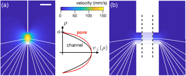
Fig.  11: : Peculiarity of pressure flow across an orifice. (a) Simulated flow velocity and streamlines across a pore with, say, radius $a=10\mathrm{nm}$ and thickness $L=a/10$ under a pressure drop $\Delta p=1\mathrm{bar}$. The scale bar is $10\mathrm{nm}$. The streamlines are spaced equally in magnitude at the center of the pore. (b) Simulated flow velocity and streamlines across a channel with same radius $a$ and thickness $L=10a$ under the same pressure drop. The scales (velocity and geometry) are the same as for (a). For readability the whole channel length is not plotted. (Center) Normalized velocity profile (perpendicular to the membrane) at the center of the membrane, comparing the channel and pore cases.

The diffusio-osmotic flow across a nanopore with vanishing thickness was recently calculated analytically by Rankin et al. ⁹³. The calculation is best performed in oblate-spheroidal coordinates, in line with a similar calculation for electro-osmosis in Ref.90. The averaged diffusio-osmotic velocity $v_{DO}$ across the pore, which is defined in terms of the diffusio-osmotic flux $Q=\pi a^{2}v_{DO}$, is proportional to $\Delta c_{s}$ the difference (and not the gradient as in Eq. (40)) of the solute concentration between the two sides of the membrane: $v_{DO}=\mu_{DO}^{\rm pore}(-k_{B}T\Delta c_{s})$. The general expression for the mobility derived in Ref.93 takes the form

$$\mu^{\rm pore}_{DO}=-\frac{2a}{\pi^{2}\eta}\int_{0}^{1}d\xi\,\xi^{2}\int_{0}^{\infty}d\nu\,\frac{e^{-{\cal U}/k_{B}T}-1}{1+\nu^{2}}$$ (59)

where ($\nu$,$\xi$) are the oblate spheroidal coordinates (iso-$\nu$ and iso-$\xi$ curves are respectively oblate spheroids and hyperboloids of revolution). This expression involves a complex spatial average of the Boltzmann weight $e^{-{\cal U}/k_{B}T}-1$, which should be compared to the corresponding simple expression in Eq. (41) for the planar case.

The above result can be simplified for certain functional forms of the potential ${\cal U}$. For example, assuming that the interaction potential ${\cal U}$ depends only on variable $\xi$ allows the mobility to be rewritten in terms of the two-dimensional interaction within the pore only as $\mu^{\rm pore}_{DO}\leavevmode\nobreak\ =\leavevmode\nobreak\ {1\over\pi a^{2}\eta}\int_{0}^{a}d\rho\rho\sqrt{a^{2}-\rho^{2}}\big{[}e^{-{{\cal U}(\rho)/k_{B}T}}-1\big{]}$ with $\rho$ the axi-symmetric distance to the center of the pore ⁹³. This expression for the mobility can be recovered thanks to the symmetry of the transport matrix Eq. (53). Indeed $\mu^{\rm pore}_{DO}$ can also be calculated in terms of the excess solute flux under a pressure driven flow: in this case the velocity profile was shown to be semicircular (and not parabolic) ^{94, 95, 96}, see Fig. 11, and the excess solute flux conveyed by the circular flow reduces to the above expression.

The complexity associated with diffusio-osmosis across an orifice is also highlighted by the predicted dependence of the mobility on the pore size $a$ and the range $\lambda$ of the interaction $\cal U$. Let us focus the discussion for the thin diffuse layer case, where $\lambda\ll a$ (we refer to Ref.93 for a full discusson). As a reference, the diffusio-osmotic mobility across a long channel with length $L$ was shown previoulsy to scale as $\mu_{DO}\sim\frac{\lambda^{2}}{\eta L}$, see e.g. Eq.(43). However, for an orifice in a thin membrane, Rankin et al. showed on the basis of Eq.(59) that the mobility exhibits a variety of non-trivial scalings, with $\mu^{\rm pore}_{DO}\sim\lambda^{\gamma}a^{1-\gamma}$, and an exponent $\gamma$ that depends on the details of the interaction potential $\cal U$. For example, for the potential discussed above, which assumes a dependence as ${\cal U}(\xi)$, one finds $\gamma=3/2$; but for a potential depending on the distance to the membrane or to the edge of the pore, then $\gamma=2$ ⁹³. In the latter case, $\gamma=2$, the diffusio-osmotic mobility scales as $\mu^{\rm pore}_{DO}\sim\lambda^{2}/a$, which corresponds to the long channel result with the length $L$ replaced by $a$. But for other values of the exponent $\gamma$ this simple rule of thumb does not apply, making the diffusio-osmotic transport across the orifice quite peculiar.

As a last comment, it is possible to extend qualitatively these results to electrolyte solutions, by assuming that the potential range $\lambda$ identifies with the Debye length. This suggests an anomalous salinity dependence for the diffusio-osmotic mobility $D_{DO}=v_{DO}/[-k_{B}T\Delta\log c_{s}]\propto c_{s}^{1-\gamma/2}$, in contrast to long channels where $D_{DO}\propto c_{s}^{0}$. The nanopore geometry may thus depart from the log-sensing behavior of diffusio-osmotic transport under salinity gradients. These results remain however to be fully assessed experimentally.

3.4 Alternative interfacial transport: thermo-osmosis

Extending on electro- and diffusio- osmosis, thermo-osmosis corresponds to fluid motion under gradients of temperature; see Fig. 12-a. Such effects were reported as early as in the 1900s ^{97, 98}. Thermo-osmosis was first rationalized in terms of thermodynamic forces by Derjaguin et al. ^{99, 54, 100}. Similarly as for diffusio-osmosis in Eq. (41) and electro-osmosis in Eq. (34), the net velocity generated far from the surface is predicted as ⁵⁴

$$v_{\infty}=\left(\frac{-2}{\eta}\int_{0}^{\infty}z\delta h(z)dz\right)\nabla\log T_{\infty}$$ (60)

where $T_{\infty}$ is the temperature far from the surface and $\delta h(z)$ is the excess specific enthalpy in the interfacial layer as compared to the bulk liquid. If the solid surface is e.g. hydrophilic, then $\delta h(z)\lesssim 0$ and the flow of water is directed toward higher temperatures, see Fig. 12 and Refs.101, 102. An interpretation of thermo-osmosis (and -phoresis) in terms of interfacial surface tension modification, and therefore Marangoni-like flow generation, has also been suggested ¹⁰³ and formalized ^{104, 105}. The transport of fluids or particles under thermal forces led to strong debates between the interfacial approach discussed above and an “energetic” approach ^{106, 107, 108}, which attempts to write the net driving force acting on a particle as the gradient of a thermodynamic quantity ¹⁰⁶. The resulting Soret coefficient – defined as the ratio between the thermophoretic mobility and particle diffusion coefficient – highlights a different dependence on the particle size as compared to the interfacial framework discussed above. Although attractive, the energetic approach was then extensively criticized  ^{107, 108}.

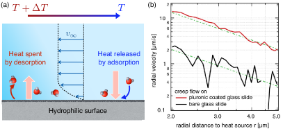
Fig.  12: : Thermo-osmosis near an interface (a) Geometry; a temperature gradient is imposed far from a hydrophilic surface. A thermal flux from the hot to the cold region is therefore installed. The interaction of water with the surface induces a force (light red arrows) that varies along the surface due to the thermal gradient, inducing a net flow. (b) Thermo-osmotic flow measured on two different surfaces (going towards the higher temperatures) as a function of the distance to the heat source. Reproduced from Ref.101 with permission from the APS, copyright 2016.

As for electro- and diffusio- osmosis, the details of the interfacial dynamics, for example slippage at the interface, is expected to strongly affect thermo-osmotic flows. This has been evidenced for example in molecular dynamics where a huge enhancement of thermo-osmosis was measured with slip ^{109, 110}, although the exact dependence of thermo-osmosis on the interfacial properties was measured to be substantially complex. ¹¹⁰ We refer to the Refs.107, 102 for more in-depth discussion on thermo-osmosis and -phoresis.

Lately thermo-osmosis has gained growing attention in terms of applications and we briefly comment here on this aspect. Many applications of the phenomenon are done in the context of thermo-phoresis, or displacement of colloidal particles under thermal gradients (in a similar way to diffusio-phoresis, see Fig. 18-a). This phenomenon was harvested to manipulate colloids and build structures ^{111, 107, 112, 113} with advanced applications in microfluidics ¹⁰¹ or towards DNA detection ¹¹⁴. Among other phenomena, it was shown that couplings between thermo- and diffusio- phoretic drivings allow to finely manipulate colloidal structures ¹¹⁵. Also, thermophoresis of molecules can provide detailed information about particles and molecules (size, charge and hydration shell) and this provide very efficient analytical tools to probe protein in biological liquids ^{116, 117}. In a different context, applications of thermo-osmosis were suggested for the recovery of water from organic waste-water ¹¹⁸, as well as for energy harvesting from thermal differences (and waste heat). ^{119, 120, 110}

3.5 Numerical simulations of (diffusio-)osmotic transport: methodologies and results

Molecular simulations have now become a highly efficient tool to explore the fundamental properties of fluids and materials. Molecular dynamics simulate the many-body dynamics of particles and molecules, either at equilibrium or far from equilibrium, submitted to various thermodynamic forces. They provide detailed information on the molecular processes at play. In the present context of studying osmotic forces and related fluxes, this represents a key opportunity to understand the fundamental and subtle origins underlying interfacial transport and how these can be affected by the microscopic details of the interface.

Simulating electro-osmosis is relatively straightforward in the sense that the effect of the electric field converts directly into an electric force acting on the suspended ions. This has led to numerous molecular dynamics studies of electro-osmosis, as well as of streaming currents, allowing to decipher a wealth of phenomena associated with transport within the electric double layer ^{121, 62}. Now, simulating diffusio- and thermo- osmosis is by far more difficult and subtle. Indeed such transport occurs under thermodynamic forces associated with the gradient of concentration or temperature, and these can not obviously be represented in terms of mechanical forces acting on the simulated particles. We discuss in this section recent developments in the numerical methodologies allowing to perform simulations of osmotic transport.

For bare osmosis, direct simulations can be performed using two explicit reservoirs with difference of solute concentration. For example such implementation was used by Kalra et al. in the study of osmosis across carbon nanotubes ¹²². This configuration has the drawback that osmosis occurs in the transient regime since the reservoirs empty/fill during the osmotic process and this limits statistics. Osmosis was later rationalized in more simple terms by simplifying the explicit membrane description to reduce it to a confining potential acting on the solute only ^{123, 124, 125}. This is the numerical pendant to the mechanical views of osmosis described in Sec. 2.4.

The numerical implementation of diffusio-osmosis in molecular dynamics is far more complex since one should be able to represent the chemical gradient in terms of a microscopic force acting on the particles. Various methods to investigate diffusio-osmotic transport were proposed in the recent literature and we discuss them now.

Using symmetry relations to infer transport coefficients –
It turns out that it is far easier to calculate the diffusio-osmotic mobility by exploiting the symmetry of the transport matrix. Recalling the general relation between fluxes and forces,

$$\left(\begin{array}[]{c}Q\\ J_{s}-c_{s}Q\end{array}\right)=\left(\begin{array}[]{cc}L_{11}&L_{12}\\ L_{21}&L_{22}\end{array}\right)\times\left(\begin{array}[]{c}-\Delta p\\ -k_{B}T\Delta\log c_{s}\end{array}\right).$$ (61)

the Onsager symmetry for the transport matrix implies that $L_{21}=L_{12}$. Accordingly, calculating the diffusio-osmotic mobility as a water flux under a concentration gradient, here $L_{12}=Q/(-k_{B}T\Delta\log c_{s})$, is therefore equivalent to calculating the excess solute flux under a pressure gradient, here $L_{21}=(J_{s}-c_{s}Q)/(-\Delta p)$ – see Fig. 13-a. The latter is far easier to implement numerically in non-equilibrium molecular dynamics (NEMD) since it requires only to generate a pressure-driven flow and measure the intergrated solute flux (or locally the velocity and solute concentration profile). This can be performed with periodic boundary conditions along the flow, so that the resulting diffusio-osmotic mobility is indeed characteristic of the liquid-solid interface under scrunity, and does not depend on e.g. entrance effects into the pore. This methodology was successfully applied to quantify the diffusio-osmotic mobility on a variety of interfaces, including superhydrophobic surfaces, graphene, and with various liquids ^{69, 70, 26, 110}. We discuss below some results of the simulations.

Equilibrium fluctuations for linear response coefficients –
Transport coefficients may also be inferred from equilibrium fluctuations by making use of Green-Kubo (GK) relations for the various mobilities. The transport coefficients introduced in the transport matrix ${\mathbb{L}}$ can indeed be written in terms of a time-correlation function of the fluctuating fluxes $Q_{i}$ at thermal equilibrium. Such formal relations are obtained thanks to linear-response theory and the fluctuation-dissipation theorem ^{126, 127, 128}. They provide generic expressions for the non-equilibrium mobilities in terms of equilibrium correlation functions in the form

$$L_{ij}=\frac{\mathcal{V}}{k_{B}T}\int_{0}^{\infty}dt\langle Q_{i}(t)Q_{j}(0)\rangle$$ (62)

where $\mathcal{V}$ is the system volume and $\{Q_{i}\}$ are the fluxes under scrutiny. The symmetry of the transport matrix originates in the time-symmetry of the underlying microscopic dynamics ²⁰. The simplest route to obtain the Green-Kubo formula for the diffusio-osmotic mobility is to consider the solute excess flux generated under a pressure drop since the latter is equivalent to a body force applied to all system particles. The linear-response formalism then immediately leads to¹²⁵

$$L_{21}=L_{21}=\dfrac{\mathcal{V}}{k_{\mathrm{B}}T}\int_{0}^{\infty}\langle(J_{s}-c_{\infty}Q)(t)Q(0)\rangle dt.$$ (63)

In the case of a channel with length $L$ and cross area ${\cal A}$, one has $L_{21}=L_{21}\equiv{{\cal A}\over L}\mu_{DO}$. We refer to Refs129, 125 for detailed derivations of these GK equations.

These GK formula allow to calculate numerically the diffusio-osmotic mobility, as well as any off-diagonal terms of Eq. (53), by estimating the correlation functions in Eq.(63) in equilbrium simulations. This approach was followed in Refs 129, 130, 125 and the resulting mobilities were successfully compared with results of NEMD simulations, as discussed below.

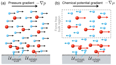
Fig.  13: : Non-equilibrium molecular dynamics of osmotic interfacial transport. Inspired from Ref.125. (a) Excess flux under pressure gradient. The pressure gradient is obtained by applying a force acting on each particle and the solute flux in excess to the bulk $J_{s}-c_{s}Q$ is measured. (b) NEMD method to simulate interfacial transport under chemical potential gradients. The chemical potential gradient is modeled as a forward force per solute particle (red) and a properly defined counter force per solvent particle (blue) such that the total force on the fluid in the bulk is zero. The local diffusio-osmotic velocity profile is directly measured.

Non-equilibrium molecular dynamics and mechanical representation of chemical gradients–
While the equilibrium approach provides proper foundations to calculate diffusio-osmosis, non-equilibrium simulations proves usually more practical to calculate transport coefficients, e.g. in terms of statistics. However, as we emphasized above, this requires to build a proper numerical scheme to implement a mechanical equivalent of the chemical potential gradient. One interesting route was suggested by Yoshida et al. in Ref.129 and then applied to electro- and diffusio- osmotic transport of electrolytes: the authors ran different simulations where forces $f_{j}$ are applied separately to each individual specie, here {solvent, anions, cations}, allowing to calculate the corresponding individual fluxes $Q_{i}$ and deduce the mobilities for the individual species $M_{i,j}=Q_{i}/f_{j}$; the electro- and diffusio- osmotic mobilities are then calculated by proper linear combinations of the mobilities of individual species, in order to deduce the electro- and diffusio- osmosis. This approach echoes directly the discussion in Sec.3.1.3, in which the electro-osmotic and diffusio-osmotic mobilities are deduced from the individual ion mobilities, defined above as $M_{\pm}$ ¹²⁹.

It is however relevant to develop numerical methods to simulate explicitly the diffusio-osmotic flows. Such a numerical scheme was recently proposed in Ref.125, in which a proper mechanical set of driving forces is applied to the system to mimick the chemical potential gradient of the solute. To do so, the scheme applies differential forces on the solute and on the solvent, see Fig. 13-b: (i) an external force $F_{\mu}$ on each solute particle in the whole system; (ii) a counter force $-[N^{B}_{s}/(N^{B}-N^{B}_{s})]\times F_{\mu}$, acting on each solvent particle. Here $N^{B}_{s}$ and $N^{B}$ are respectively the number of solute particles and the total number of particles in a properly defined bulk region (“sufficiently” far from the surface). The counter force is set to ensure a force free balance in the bulk volume. Most important, it can be verified that applying linear-response theory to the system with this set of forces allows one to show that the resulting diffusio-osmotic mobility does identify with the GK relation in Eq.(63): this therefore fully validates the theoretical foundations of the proposed numerical scheme. The corresponding effective chemical potential is then related to the applied external force $F_{\mu}$ via

$$-\nabla_{x}\mu=F_{\mu}\frac{N^{B}}{N^{B}-N^{B}_{s}}.$$ (64)

This approach leads as expected to a velocity profile exhibiting a strong gradient within the interfacial layer, and then a plug flow far from the surface. The deduced diffusio-osmotic mobility obtained from the NEMD scheme was checked to be identical to both the equilibrium GK results and those obtained from the excess flux under pressure-driven flow introduced above ¹²⁵.

Some difficulties with the microscopic stress tensor–
The continuum approach, as described above, allows one to predict diffusio-osmotic transport in terms of a surface pressure gradient. In a different approach, it is accordingly tempting to obtain the diffusio-osmotic flow by a direct numerical calculation of the local microscopic pressure in the fluid. However, as was demonstrated by Frenkel and collaborators in a series of papers ^{131, 132, 133, 134}, a major difficulty in this approach is that there is no unique expression for the local microscopic pressure tensor (e.g. in terms of the position and velocities of individual particles and the microscopic forces acting on them). Accordingly various microscopic definitions of the pressure tensor lead to different numerical results. Such difficulty was evidenced for diffusio-osmotic flows¹³², but also for thermo-osmotic flows ^{133, 134}.

Some results of simulations–
Simulations have allowed to gain much insights into diffusio-osmotic transport. Various fluids, e.g. Lennard-Jones fluids, but also with electrolytes and water-ethanol mixtures, and various interfaces were considered, hydrophilic or hydrophobic surfaces, graphene, superhydrophobic surfaces, etc. Among highlighted effects one may quote the impact of hydrodynamic slippage of the fluid at the surface, which does boost considerably the diffusio-osmotic mobility on hydrophobic ⁶⁹ and graphene surfaces ¹²⁵, and even more on super-hydrophobic surfaces ⁷⁰. The enhancement of the diffusio-osmotic mobility scales typically like the ratio between the (effective) slip length and the interfacial length, as mentionned in the previous sections.

Simulations also give some insights on the local diffusio-osmotic velocity profile and its relation to the concentration profiles. Within the continuum framework discussed in the previous section, the velocity profile is obtained simply by integration of the Stokes equation of motion in Eq.(39), with the pressure expression given in Eq.(38). Simulations actually show usually a very good agreement between the continuum prediction and the velocity profiles measured in the NEMD simulations, giving strong support to the continuum description. Such an agreement may be considered as surprising in view of the strong velocity gradients occurring on length scales in the range of a few molecular size. However the Stokes equation is known to be surprisingly robust down to molecular lengthscales ⁶² and this explains its success in predicting diffusio-osmotic flows.

Finally, the continuum framework allows one to relate the diffusio-osmotic mobility to the concentration profile, and more particularly to its first spatial moment, see Eq.(41). It is accordingly tempting to relate – as for Marangoni effects – the amplitude of diffusio-osmotic transport to the adsorbed quantity, defined as $\Gamma=\int dz\,(c_{s}(z)-c_{\infty})$. The latter is directly connected to the surface tension via the Gibbs-Duhem relation. The adsorbed quantity $\Gamma$ provides in most cases a good estimate for the diffusio-osmotic mobility and its sign. However – as mentioned earlier – for complex concentration profiles the relation was found to be more complex than this simple rule of thumb (for example for water-ethanol mixture at interfaces ²⁶).

4 Osmosis beyond van ’t Hoff

4.1 Advanced osmosis and nanofluidics

The previous section highlighted molecular insights into osmotic phenomena, unveiling the underlying driving forces at play. However such perspectives also suggest possible extensions to obtain more advanced osmotic transport beyond the linear framework presented before. In this section we discuss osmotic transport across channels with more complex geometries involving symmetry breaking, or active parts. Our objective in this section is to show that it is possible to extend simple osmosis beyond the van ’t Hoff paradigm and design advanced functionalities resulting in non-linear and active transport.

In this context it is interesting to observe that in biological species (bacteria, archaea, fungi, …) many membrane channels do achieve advanced functionalities in order to regulate osmosis: for example rectified osmosis ¹³⁵ –e.g. an osmotic flow with a non-linear dependence on the concentration gradient–, or gated osmosis to prevent lysis and survive osmotic shocks in mechanosensitive channels ³ (with diffusio-osmosis identified as a potential mechanism for the gating mechanism in deformable structures ¹³⁶). These few examples highlight the possibility of going far beyond the van ’t Hoff paradigm, thanks to properly designed (active) nanochannels.

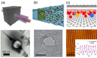
Fig.  14: : From nanoscale to ȧngström scale pores. (a) Reproduced from Ref.73. (Top) Molecular dynamics representation of water flowing through a transmembrane multi-wall boron-nitride nanotube and (bottom) Transmission electron microscope (TEM) picture of its experimental counterpart. (b) (top) Molecular dynamics representation of a nanopore in a mono-layer MoS₂ membrane (in blue and yellow) and the salt (green and red) in solution and (bottom) TEM picture of its experimental counterpart, a 5 nm pore. Reproduced from Ref.74 with permission from Springer Nature, copyright 2016. (c) (top) Molecular dynamics representation of water and ions (orange and blue) flowing through a graphene slit with $7$ ȧngström spacing. (Courtesy from Timothée Mouterde) (bottom) AFM image of bilayer graphene spacers on top of the bottom graphite layer. Inset: Height profiles yield an estimate of 7Åfor the thickness of spacers made from 2 layers of graphene or 1 layer of MoS₂ (the blue line shows the scan position for the corresponding trace in the inset). Reproduced from Ref.137 with permission from AAAS, copyright 2017.

We believe that the advent of nanofluidics has a key role to play in this regard, in order to identify new types of behaviors which could be scaled-up to macroscopic membranes. The new opportunities brought by nanofluidics in terms of the variety of nanoscale geometries and materials, combined with state-of-the-art experimental instrumentation, allows one to fabricate and investigate fundamentally the transport in ever smaller channels, with ever more complex and rich behaviors. Carbon nanotubes, down to nanometric sizes ^{73, 138, 139, 140} can now be manipulated and inserted in devices were water is flown through – see Fig.  14-a. Single nanopores can be carved or etched in membranes that are only an atomic layer thick ⁷⁴ and may be accordingly functionalized ¹⁴¹, see Fig. 14-b. It is also now possible to fabricate ȧngström scale slits using graphene sheets as spacers, reaching confinement thicknesses down to $\sim 3$ Å ^{142, 143} – see Fig. 14-c.

Such nanofluidic technologies offer new possibilities in the context of osmotic transport. They allow nearly molecular scale designs, leading to various nanofluidic-specific effects which may be key assets for new separation techniques and water filtration: from specific ion exclusion effects ^{144, 138, 143, 140, 87} with a number of anomalous ionic effects to be investigated ¹⁴⁵, to extremely fast permeation of water, in particular through carbon nanotubes ^{146, 147, 148, 139, 140}. Also new types of nanoscale membranes have also emerged recently, offering new designs as compared to traditional membranes: for example, with dedicated patterns of hydrophilic and hydrophobic regions ¹⁴⁹; or tailor-designed DNA origami channels ^{86, 150}, and – last but not least – the multilayer membranes of graphene (so-called graphene oxide membranes) ^{151, 152, 75}.

This constitutes a new and exciting playground, in which osmotic phenomena may (and should) flourish in various forms. We discuss in the next paragraphs two such examples: the development of osmotic diodes, and an active counterpart of osmosis, which both lead to tunable osmotic driving beyond van ’t Hoff.

4.2 Osmotic diodes and osmotic pressure rectification

One of the successes of nanofluidics was to demonstrate the possibility to design diodes for ionic transport, in full analogy with their electronic counterpart ^{85, 153, 62}. This takes the form of a non-linear and rectified response for the ionic current versus the applied voltage. Typically an ionic diode behavior manifests itself in channels with an asymmetric design, e.g. an asymmetric surface charge or an asymmetric geometry. Such behavior is expected to occur in the regime where the Dukhin number is of order one and asymmetric along the channel ¹⁵⁴: the Dukhin number is defined here as $Du=\Sigma/c_{s}h$, where $\Sigma$ is the surface charge density, $c_{s}$ the bulk salt concentration and $h$ a characteristic channel dimension. It quantifies the importance of surface versus bulk electric conduction. As such ionic diodes may find interesting applications to boost osmotic power generation under salinity gradients, see Ref.75 and Sec. 6.3.

Now, coming back to osmosis, the asymmetry of the design may be expected to yield an asymmetric interaction of the membrane with the electrolyte, hence an asymmetric push on the liquid. It was shown in Ref.50 that such asymmetric geometry – depicted in Fig. 15-a – results in an osmotic diode, with a rectified osmotic pressure versus the concentration gradient (non linear dependence), furthermore tunable by the applied electric field.

The description builds on the previous mechanical views of osmosis, in Sec. 2.4. The Stokes equation for fluid motion writes

$$0=-\bm{\nabla}p+\eta\nabla^{2}\bm{u}+\rho_{e}(-\bm{\nabla}V_{e}),$$ (65)

with $\rho_{e}=e(c_{+}-c_{-})$ the charge density, $c_{\pm}$ is the concentration of positive and negative ions (assumed here as monovalent for simplicity) and $V_{e}$ is the electric potential. Following the same steps as in Sec. 2.4 to integrate the fluid equations of motion in the channel, the general relation between flow and pressure takes the expression

$$Q=\mathcal{L}_{\rm hyd}\times{-\Delta[p-\Pi_{\rm app}]}$$ (66)

where $\mathcal{L}_{\rm hyd}$ is the channel permeance introduced above. The apparent osmotic pressure between the two sides of the channel is accordingly defined as

$$\Delta\Pi_{\rm app}=\frac{1}{\mathcal{A}}\int\int{d\mathcal{A}}dx\,\rho_{e}\times(-\bm{\nabla}V_{e})$$ (67)

with $\mathcal{A}$ the cross section of the pore, $L$ its length. The ion concentration profiles obey the Poisson-Nernst-Planck equations, coupling the diffusive dynamics to the applied electric forces. In spite of the expected non-linear dependence of the osmotic pressure in terms of driving forces, the symmetry in the force balance and ionic transport equations, which was highlighted in Sec. 2.4 and Eq. (28) for the simplest geometry, still holds. There is accordingly a linear relation between the apparent osmotic pressure in Eq. (67) and the total surface ion flux $j_{s}$:

$$\Delta\Pi_{\rm app}=k_{B}T\Delta c_{s}+j_{s}\times{L\over D}.$$ (68)

It is therefore expected that the rectifying behavior in the ion flux, akin to the current diode, thus translates into a rectifying osmotic pressure.

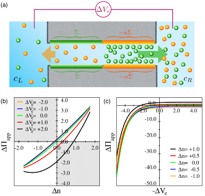
Fig.  15: : Osmotic rectification in an osmotic diode. (a) A nanochannel presents an asymmetric surface charge with $\Sigma>0$ and $-\alpha\Sigma$ on the other side with $\alpha\neq 1$. The ions are therefore submitted to an asymmetric force (between one side and the other, in colored arrows) that drives the osmotic flow. Inspired from Ref.50. Apparent osmotic pressure $\Delta\Pi_{\rm app}$ versus (b) salinity gradient $\Delta n=n_{R}-n_{L}$ (where $n_{i}=c_{i}/c_{0}$ is a normalized concentration) and versus (c) applied voltage drop $\Delta V_{e}=V_{R}-V_{L}$ (normalized by $k_{B}T/e$) as obtained from an analytical solution for the flows of all species in the nanochannel. (b) and (c) are reproduced from Ref.50 with permission from the APS, copyright 2013. More information can be found in Ref.50.

Solving the full equations in the geometry presented in Fig. 15-a yields a fluid flux: ⁵⁰

$$Q=\mathcal{L}_{\rm hyd}[\sigma k_{B}T\Delta c_{s}-\Delta p]+Q_{S}[\Delta c_{s}]\left(\exp\left(\frac{e\Delta V_{e}}{k_{B}T}\right)-1\right)$$ (69)

where the reflection coefficient $\sigma$ is now a non-linear function of the concentrations in both reservoirs and $Q_{S}$ plays the role of a “limiting fluid flux” ⁵⁰. The apparent osmotic pressure $\Delta\Pi_{\rm app}=Q/\mathcal{L}_{\rm hyd}$ is plotted in Fig. 15. The rectification and diode behavior versus concentration is weak for zero voltage but strongly enhanced for higher applied voltage bias.

Examples of permeability rectification are actually numerous in the biological world. They are harnessed e.g. in plant cells ¹³⁵ or in animal cells ^{155, 156, 157}. Surprisingly in all the studies that we are aware of, entering flows are notably larger than outer flows, and up to 10 times higher in some mammalian fibroplasts ¹⁵⁷. It is fascinating to see how most cells are therefore adapted to fill in faster than they would swell under the same conditions, probably with a link to survival strategies. We highlight that rectified osmotic flows could be used in a variety of fields. In fact, Fig. 15-b and the results reported in Ref.50, demonstrate that water may be flown against the natural osmotic gradient, with water flowing to the high salinity reservoir, depending on the voltage applied. Furthermore, under an oscillating electric field, with proper conditions, this induced water flow against the natural osmotic gradient will be maintained. This opens new perspectives e.g. for advanced water purification strategies and active filtration with oscillating fields, as we discuss later.

4.3 Towards active osmosis

We discuss now a second class of examples of osmotic phenomena that goes beyond the van ’t Hoff paradigm. As we exhaustively discussed, the idea of osmosis is closely related to semi-permeability and sieving – with the membrane playing the role of a simple colander. However one may consider how the osmotic pressure builds up in membranes with time-dependent pores: a pore which opens and closes over time – see Fig. 16 – will exhibit a time-dependent size exclusion and sieving is thus expected to generate an intermittent osmotic push on the fluid. The resulting osmotic pressure is expected to be some time-average of the push, which remains to be properly defined. But injecting energy at the pore scale – here via the time-dependent opening of the pore – may also lead to far-from-equilibrium behaviors, allowing possibly to bypass the entropy bottleneck. Osmosis across dynamically stimulated pores is therefore a subtle problem, which requires proper microscopic foundations. Beyond the fundamental question, adding the sieving frequency as a new tuning parameter may improve separation and selectivity properties of the membranes  ^{158, 159}.

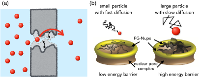
Fig.  16: : Osmosis through out-of-equilibrium pores. (a) Illustration of a pore with a time-dependent shape, where the inner pore size may be either smaller either larger than the typical solute size. (b) Reproduced and adapted from Ref.160 with permission from Springer Nature, copyright 2016. Representation of the spatiotemporal motion of grafted phenylalanine-glycine nucleoporins (FG-Nups) inside the selectivity filter of the nuclear pore complex. Small (resp. large) particles that diffuse fast (resp. slow) see effectively the FG-Nups as static leaving small openings (resp. moving and everywhere) and therefore encounter only a "small" energy barrier for translocation (resp. large).

The question of dynamic osmosis actually arises naturally in biological pores, e.g. ion channels, since their shape is affected by thermal fluctuations or demonstrates out-of-equilibrium motion ¹⁶¹. The question of out-of-equilibrium osmosis was discussed in the literature in the 1980s ¹⁶² and a few molecular dynamics studies were pursued ^{163, 164, 161}, usually with a focus on the specificities of the biological channels under scrutinity. In fact, temporal dynamics of biochannels are strongly believed to be connected to the selectivity properties of the channel. For example, the fluctuations of the refined structure of the selectivity filter of the KcsA channel is believed to be a key factor for extremely refined passage of the potassium ion ¹⁶¹. Further, such temporal dynamics of the structure may provide an efficient alternative to simple steric sieving for selectivity. This was noticed in the nuclear pore complex ¹⁶⁰, where particles see an effective translocation barrier which is dependent on their diffusion properties (see Fig. 16-b).

To our knowledge, there is no general framework discussing the concept of “dynamic osmosis”. Several simple models were considered recently by the authors in  Refs.158, 159. Here we illustrate a few basic concepts underlying this active osmosis process and the opportunities that it offers.

In line with our previous discussion of osmotic phenomena, it is particularly fruitful to address the question under the perspective of the mechanical insights, where the pore with fluctuating shape is modeled as a time-dependent energy barrier, say ${\cal U}(x,t)$, using similar notations as previously. The average osmotic force acting on the fluid is again obtained in terms of the force acting on the fluid integrated over the channel size and averaged over time. It writes within this framework

$$\Delta\Pi_{\rm app}=\langle\int dx\,c_{s}(x,t)\times(-\nabla_{x}{\cal U}(x,t))\rangle_{t}.$$ (70)

where here $\langle\cdot\rangle_{t}$ denotes a time average. As for the static (passive) case, the Smoluchowski equation for the solute allows one to rewrite the apparent osmotic pressure in terms of the solute flux across the fluctuating barrier:

$$\Delta\Pi_{\rm app}=k_{B}T\Delta c_{s}+\langle j_{s}\rangle_{t}\times{L\over D_{s}}.$$ (71)

It is interesting to note that the concept of osmotic force $\Delta\Pi_{\rm app}$ connects directly to the question of translocation of solute molecules across a fluctuating barrier – via the solute surface flux $j_{s}$. That specific question was actually the topic of an exhaustive literature in the context of ratchets, molecular motors, or stochastic resonance ^{165, 166}. Numerous counter-intuitive consequences were highlighted, both theoretically and experimentally, like directed motion, “uphill” transport against gradients, enhanced translocation, etc. Accordingly the previous symmetry relation Eq. (71) shows that the existence of a finite flux $\langle j_{s}\rangle_{t}$, with possibly unconventional dependencies on the concentrations in the reservoirs, will have consequences on osmotic transport, i.e. leading to flow of the suspending fluid itself and not only solute motion.

To illustrate this behavior, it is instructive to consider a simple example, made of an asymmetric membrane as in Fig. 17, which oscillates in time as an “on/off” process over a time interval $\tau/2=\pi/\omega$. When “on”, the barrier height is considered as much larger than the thermal energy. This process bares similarities with the ratchet process in Ref.167 and subsequent references, where solute pumping was demonstrated.

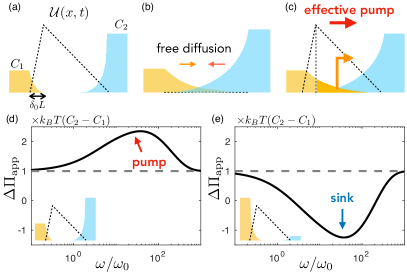
Fig.  17: : Active membrane as a pump (or sink). (a) An asymmetric potential barrier (representing the membrane acting on the solute) separates two solute reservoirs with different concentrations. (b) As the barrier is temporarily lowered, the solute may diffuse inwards from both sides. (c) If the barrier is risen back, the solute that has diffused beyond the maximum point of the energy barrier will be carried to the other side. In the example shown here, more solute from the lower concentration side has traversed beyond the maximal point. This solute is then transported to the highly concentrated side. The active membrane therefore acts as a pump. (d) and (e) Apparent rejection coefficient as obtained from the on/off energy barrier model described in the text ¹⁶⁸. The normalizing frequency is $\omega_{0}=D_{s}/L^{2}$, and the asymmetry parameter is here $\delta_{0}=0.1$. Insets indicate the solute concentration on both sides; $\Delta c_{s}=C_{2}-C_{1}$; for (d), $C_{1}=0.4C_{0}$ and $C_{2}=C_{0}$ where $C_{0}$ is some arbitrary concentration and for (e) $C_{1}=C_{0}$ and $C_{2}=0.1C_{0}$.

In elementary terms, when the barrier is “off”, solute molecules from both sides diffuse freely (see Fig. 17-b). Now, when the barrier is back “on”, solute that has crossed the maximum point of the barrier will slide down to the opposite side (see Fig. 17-c). This process leads to a finite flux of solute averaged over a period, $\langle j_{s}\rangle_{t}$, which can be exactly calculated in the simple model considered, see Ref.168. For example, in the quasi-static (low frequency) regime, the averaged flux reduces in this simple system to

$$\langle j_{s}\rangle_{t}\underset{\omega\rightarrow 0}{\sim}L\omega\times\left[C_{2}\times\delta_{0}-C_{1}\times(1-\delta_{0})\right],$$ (72)

with $C_{1}$ and $C_{2}$ the solute concentrations in both reservoirs and $\delta_{0}$ the potential asymmetry, see Fig.17. Beyond the specific expression (restricted to this specific regime and model), this result highlights the possibility of uphill solute transport (pumping against concentration gradients) or enhanced solute flux, depending on the direction of the concentration gradient versus the pore asymmetry. This behavior is summarized in Fig. 17-d-e.

Now inserting this result for the flux in Eq. (71), one therefore predicts highly counter-intuitive behaviors for the osmotic pressure, i.e. the driving force acting on the fluid. In Fig. 17-d-e, we have introduced and plotted the apparent osmotic pressure

$$\Delta\Pi_{\rm app}=k_{B}T(C_{2}-C_{1})+{k_{B}TL\over D_{s}}\times\langle j_{s}\rangle_{t}(C_{1},C_{2},\omega)$$ (73)

based on the full solution of the simplistic previous model. Notably this plot highlights the possibility of “resonant osmosis” for a characteristic frequency (in the form of an extremum of $\sigma_{\rm app}$), but this simple model also suggests that – depending on the direction of the potential asymmetry against the concentration gradient – the rejection may be larger than unity (pumping regime) or even decrease towards negative values ¹⁶⁸.

This points to a wealth of intriguing behaviors for osmotic phenomena, which were barely explored up to now. As emphasized above, the recent development of nanofluidics suggests many routes to develop such active pores in artificial channels, e.g using voltage-gated nanochannels ^{169, 170, 171, 172} or UV light ¹⁷³ or stimulated surface chemical reactivity ^{174, 175}. Other externally controlled existing devices include thermally responsive nanochannels ^{176, 177}. The challenge awaiting is to achieve such active control in yet smaller devices to significantly impact water or ion transport.

The foundations of active osmosis remain therefore to be properly investigated. The present discussion is merely an appetizer to illustrate the abundance of “exotic” behaviors which could be unveiled in this context.

5 From diffusio-phoresis of particles to active matter

The previous sections showed how gradients of solutes induce fluid motion in the presence of an interface via the diffusio-osmotic phenomenon. Symmetrically when a (solid) particle is suspended in a quiescent fluid, gradients of solute will induce motion of the particle. This motion, called “diffusio-phoresis”, relies on the very same osmotic driving forces, occurring within the interfacial layer at the particle boundary. The idea to transport large particles harnessing osmotic forces appeared first in the Russian literature with the works of Derjaguin and Dukhin ^{55, 56, 99} and was more thoroughly investigated in the 1990s ^{178, 179, 79}. We refer to the review by Anderson in Ref.54 for a dedicated discussion of the underlying transport mechanisms and some of its subtle features.

Diffusio-phoresis and its consequences have gained renewed interest for the last decade, highlighting an increasing number of situations where this phenomenon is shown to play a role, as well as dedicated applications in various domains. Basically diffusio-phoresis occurs whenever there is a gradient of solute or of a mixture of solutes and such situations are ubiquitous ^{180, 181}. Here we summarize the main elements of the phenomenon and focus on a number of elementary implications. More explicit applications will be discussed in the next section, Sec. 6.

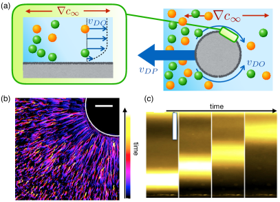
Fig.  18: : From osmosis to phoresis. (a) Under a concentration gradient, a particle is put into motion via diffusio-osmosis occurring at its surface. (b) Time-stamped stream lines of decane droplet migration towards a hydrogel beacon initially loaded with sodium dodecyl sulfate (SDS), acting as a long-range solute source. Adapted from Ref.182 with permission from the United States National Academy of Science, copyright 2016. The scale bar is 100 $\mathrm{\mu}m$. (c) Diffusio-phoretic transport of fluorescent $\lambda$-DNA under a LiCl gradient ($\Delta c_{s}=100mM$ over a range of $800\mathrm{\mu}m$, highest concentration being up), scale bar is 100 $\mathrm{\mu m}$. Images at 100, 150, 200 and 300 s. Adapted from Ref.77.

5.1 E pur si muove: from diffusio-osmosis to diffusio-phoretic motion

The diffusio-phoretic velocity of a particle under a (dilute) solute gradient writes as ⁵⁴

$$\bm{v}_{DP}=\mu_{DP}\times(-k_{B}T\bm{\nabla}c_{\infty})$$ (74)

Physically the phenomenon at stake is sketched in Fig. 18: the solute gradient at the solute surface induces a diffusio-osmotic slip velocity of the fluid (relative to the solid particle) beyond the interfacial diffuse layer; the particle is put in motion in order to precisely negate the corresponding velocity. For spherical particles, the value of the mobility $\mu_{DP}$ defined in Eq. (74) identifies with minus the corresponding diffusio-osmotic mobility, as given previously in Sec. 3.1:

$$\mu_{DP}=-\mu_{DO}.$$ (75)

For example, for a solute interacting via a potential $\cal U$ with the particle, the diffusio-phoretic mobility is minus the mobility in Eq. (41):

$$\mu_{DP}=-\mu_{DO}=-\frac{1}{\eta}\int_{0}^{\infty}\,z\,\left(\exp\left(\frac{-\mathcal{U}(z)}{k_{B}T}\right)-1\right)dz.$$ (76)

Interestingly, provided the value for the diffusio-osmotic mobility is constant over the particle’s surface, it was shown by Morrison that this result holds for any particle shape (the argument is valid for any interfacially driven transport ^{183, 54}).

5.1.1 Phoresis in the thin layer limit

Summarizing briefly the derivation, Eq. (76) is obtained by separating the diffusio-osmotic driving, which occurs at the particle surface within the diffuse layer of thickness $\lambda$, and the far-field flow occurring beyond the diffuse layer. Following the prediction in Sec. 3.1, the near-field diffusio-osmotic flow results in a diffusio-osmotic “slip” velocity of the fluid relative to the particle, with amplitude $\mu_{DO}\times(-k_{B}T\bm{\nabla}c_{s})_{t}$, where the index $t$ refers to the tangential component along the particle surface. The concentration gradient in the vicinity of the surface $(\bm{\nabla}c_{s})_{t}$ is related to the far concentration field $c_{s}$. It obeys Ficks’ equation $\nabla^{2}c_{s}=0$ together with the boundary condition at infinity fixing the concentration gradient, $c_{s}(r\rightarrow\infty)\simeq z\nabla c_{\infty}$, with $z$ the coordinate along the direction of the gradient. This gives (in spherical coordinates):

$$c_{s}(r,\theta)=R\,\nabla c_{\infty}\left({r\over R}+{1\over 2}\left(R\over r\right)^{2}\right)\times\cos\theta$$ (77)

outside of the diffuse layer; with $r,\theta$ the spherical coordinates. Back to the flow, the velocity field outside the diffuse layer obeys the Stokes equation

$$\eta\bm{\nabla}\bm{v}-\bm{\nabla}p=0,$$ (78)

with the boundary conditions on the particle given by the tangential slip velocity and at infinity given by the uniform flow field

$$\bm{v}(r=R^{+})=-{\frac{3\sin\theta}{2}}v_{slip}\,\bm{t},\,\,\;\&\,\,\;\bm{v}(r\rightarrow\infty)=-\bm{v}_{DP}$$ (79)

in the particle frame of reference; $v_{slip}=\mu_{DO}\times(-k_{B}T\nabla c_{\infty})$, $R^{+}\approx R+\lambda$ denotes the position on the particle surface but located beyond the diffuse layer (here considered as infinitesimal); $\bm{t}$ is the tangential vector on the particle’s surface. To lowest order, the solution to the previous equations results in a flow dominated by a Stokeslet

$$\begin{split}v_{r}&=-v_{DP}\cos\theta+{F\over 4\pi\eta}{\cos\theta\over r}+{\cal O}\left({1\over r^{3}}\right)\\ v_{\theta}&=v_{DP}\sin\theta-{F\over 8\pi\eta}{\sin\theta\over r}+{\cal O}\left({1\over r^{3}}\right)\end{split}$$ (80)

where $F=6\pi\eta R({v}_{DP}+v_{slip})$. As can be easily verified, $F$ identifies with (minus) the force acting on the particle. At steady-state, the particle is moving with a constant velocity $v_{DP}$ and no force acts on it. Accordingly, the diffusio-phoretic velocity $\bm{v}_{DP}$ is fixed by imposing $F=0$ and this results in Eq. (74). This shows implicitly that the far velocity profile scales like $1/r^{3}$ and can be rewritten as in Ref.54

$$\bm{v}_{l}({\bm{r}})={1\over 2}\left({R\over r}\right)^{3}\left[3{{\bm{r}}{\bm{r}}\over r^{2}}-\bm{I}\right]\cdot\bm{v}_{DP}.$$ (81)

where we came back to the lab frame of reference, $\bm{v}_{l}({\bm{r}})=\bm{v}({\bm{r}})-\bm{v}_{DP}$. Accordingly, the hydrodynamic interaction between particles undergoing diffusio-phoretic transport is weak, in contrast to e.g. gravity driven transport where the fluid velocity scales like $1/r$ far from the particle. This has important consequences for the phoretic transport in confinement ^{54, 184, 185}.

5.1.2 Osmotic force balance on particles

Let us come back to the force balance underlying diffusio-phoresis. We emphasized above that diffusio-phoresis, like any interfacially driven transport, is a force-free motion: the particle moves without any force acting on it, i.e. the global resulting force acting on the particle vanishes ⁵⁴. This has counter-intuitive consequences and led to various mis-interpretations and debates concerning osmotically-driven transport of particles ^{186, 187, 188, 189, 190, 191}, in particular in the context of phoretic self-propulsion (see Sec. 5.3 and Ref.192). We thus take the proper space here to discuss the osmotic force balance.

A naive interpretation of diffusio-phoresis is that the particle velocity $v_{DP}$ under a solute gradient results from the balance of Stokes’ viscous force $F_{v}=6\pi\eta Rv_{DP}$ and the osmotic force resulting from the gradient of the osmotic pressure integrated over the particle surface, hypothetically scaling as $F_{osm}\sim R^{2}\times R\nabla\Pi$. Balancing the two forces one finds a phoretic velocity behaving as $v_{DP}\sim R^{2}{k_{B}T\over\eta}\nabla c_{s}$. Looking at the expression for the diffusio-phoretic mobility in the thin layer limit, Eqs. (74) and (76), the latter argument does not match the previous estimate by a factor of order $(R/\lambda)^{2}$, where $\lambda$ is the range of the potential of interaction between the solute and the particle.

The difference between the two scalings originates in the fact that for interfacially driven motion, the velocity gradients occur mostly over the thickness $\lambda$ of the diffuse layer, and not on the particle size $R$, as e.g. for the Stokes flow. More fundamentally, this raises the question of how osmotic pressure is expressed: the existence of a difference of solute concentration between the two sides of the colloidal particle does not obviously imply the existence of a corresponding osmotic pressure and this belief led to much confusion. The argument above based on the global force balance is globally flawed and needs to be properly clarified. In his exhaustive work in Ref.191 following the debate of Refs.186, 187, 188, 189, 190, Brady tackled the question based on a “micromechanical” analysis of the solute and solvent transport in the presence of the colloidal particles.

However, in order to properly solve the riddle and reconcile the various approaches, one needs to go into the details of the force distribution and write properly the force balance on the particle undergoing diffusio-phoretic transport. It is accordingly interesting to relax the hypothesis of a thin diffuse layer, and consider more explicitly the transport inside the diffuse layer, as was explored by various authors, using e.g. controlled asymptoptic expansions ^{193, 194, 195}.

General results for the hydrodynamic flow and mobility can be obtained without assuming a thin diffuse layer. We consider that the interaction between the solute and the particle occurs via a radially symmetric potential ${\cal U}(r)$, so that the Stokes equations now writes

$$\eta\bm{\nabla^{2}}\bm{v}-\bm{\nabla}p+c_{s}(\bm{r})(-\bm{\nabla}{\cal U})=0.$$ (82)

The boundary conditions are now replaced by the no-slip boundary condition on the particle’s surface, as well as the prescribed velocity at infinity (in the frame of reference of the particle):

$$\bm{v}(r=R)=\bm{0}\,\,\;\mathrm{and}\,\,\;\bm{v}(r\rightarrow\infty)=-\bm{v}_{DP}$$ (83)

The concentration profile obeys a Smoluchowski equation in the presence of the external potential ${\cal U}(r)$, in the form

$$0=-\bm{\nabla}\cdot\left[-D_{s}\bm{\nabla}c_{s}+\lambda_{s}c_{s}(-\bm{\nabla}{\cal U})\right]$$ (84)

with the boundary condition at infinity accounting for a constant solute gradient $c_{s}(r\rightarrow\infty)\simeq r\cos\theta\nabla c_{\infty}$ (convective transport is neglected here). Given the symmetry of the problem, the solution takes the general form $c_{s}(r,\theta)=c_{0}(r)\cos\theta$, with $c_{0}$ scaling with the gradient at infinity as $c_{0}\propto R\nabla c_{\infty}$. Altogether this is a self-consistent equation for the solute concentration field. It should therefore be considered as a source term for the fluid transport Eq. (82). For large distances to the particle ($r\gg\lambda$), it reduces to the previous result in Eq. (77).

Interestingly, the solution of Eq. (82) for the velocity profile can be calculated exactly for any radially symmetric potential ${\cal U}(r)$, by extending textbook techniques for the Stokes problem in Ref.96; see also 196 for a related calculation in the context of electro-phoresis. It can be demonstrated that the solution for $\bm{v}(\bm{r})$ still takes the same form as in Eq. (80), but the force along the axis of the gradient appearing in the Stokeslet term ($v\sim F/r$) term now takes the expression

$$F=6\pi R\eta v_{DP}-\pi R^{2}\int_{R}^{\infty}c_{0}(r)(-\partial_{r}{\cal U})(r)\times\varphi(r)dr$$ (85)

with $\varphi(r)={2\over 3}\left(3{r\over R}-2\left({r\over R}\right)^{2}-{R\over r}\right)$ a dimensionless function, the factor ${2\over 3}$ originating from the angular average. The diffusio-phoretic velocity results from the force-free condition, $F=0$, and therefore it writes

$$v_{DP}=\frac{\pi R^{2}}{6\pi\eta R}\int_{R}^{\infty}c_{0}(r)(-\partial_{r}{\cal U})(r)\times\varphi(r)dr$$ (86)

Remembering that $c_{0}(r)\propto R\nabla c_{\infty}$, this equation generalizes the previous result obtained in the thin layer limit.

At first sight, Eqs. (85) and Eq. (86) appear as a force balance between the Stokes friction $6\pi R\eta v_{DP}$ and the osmotic force, here written in terms of the local force $c_{0}(r)(-\partial_{r}{\cal U})(r)$ integrated over the particle surface (and potential range). The latter represents the push of the solute molecules on the particle. Actually, Eq. (86) is very similar to Eq. (2.7) in Ref.191, with the $r$-dependent term $\pi R^{2}\times\varphi(r)$ replaced in Ref.191 by the prefactor $L(R)$. However the integrated “osmotic push” is weighted here by the local factor $\varphi(r)$ (in contrast to Ref.191) and this detail actually changes the whole scaling for the mobility.

Indeed in the thin diffuse layer limit, with $r-R\sim\lambda\ll R$, then one may expand $\varphi(r)\simeq-2(r-R)^{2}/R^{2}$, while the concentration profile $c_{0}(r)$ can be approximated as

$$c_{0}(r)\simeq R\nabla c_{\infty}\times\left[{r\over R}+{1\over 2}\left({R\over r}\right)^{2}\right]\exp[-{\cal U}(r)/k_{B}T].$$ (87)

One may then verify that the above Eq. (86) indeed reduces to the results in Eqs. (74) and (76) predicted by the thin layer approach. In other words, the weight $\varphi(r)\sim\lambda^{2}/R^{2}$ is a signature of the fact that the velocity gradients occur on the potential width $\lambda$ and not on the particle size $R$. An osmotic pressure is indeed expressed at the particle’s surface and yields diffusio-phoretic transport, but in a very subtle way which does not reduce to considering only the direct solute force. This corrects the naive argument suggested at the beginning of the section.

The exact calculation above also allows one to gain key insight into the local force acting on the particle. The latter is the sum of the hydrodynamic shear force, normal pressure and direct interaction with the solute. Using the exact results for the velocity profile in the thin layer regime, $\lambda\ll R$, one predicts

$$\begin{split}f_{r}&=3L_{s}R^{2}k_{B}T\nabla c_{\infty}\cos\theta\\ f_{\theta}&=\frac{3}{2}L_{s}R^{2}k_{B}T\nabla c_{\infty}\sin\theta\end{split}$$ (88)

where $L_{s}=\int_{R}^{\infty}\left(e^{-\beta\mathcal{U}(x)}-1\right)dx$ has the dimension of a length and quantifies the excess adsorption on the interface. Eq. (88) can be recovered easily with a simplistic argument: one expects this osmotic force to scale as $\mathcal{V}_{\rm int}\nabla\Pi=\mathcal{V}_{\rm int}\nabla(k_{B}Tc_{\infty})$ where $\mathcal{V}_{\rm int}$ is the interaction volume. Writing $L_{s}$ the typical interaction lengthscale we have $\mathcal{V}_{\rm int}\approx 4\pi R^{2}L_{s}$, leading accordingly to Eq. (88). While the integrated total force does vanish as expected, the osmotic gradients do generate an inhomogeneous local tension on the surface of the particle, as plotted in Fig. 19-a. Accordingly, if one considers that the particle is elastically deformable, such tensions would generate a deformation of the particle following the shape sketched in Fig. 19-b.

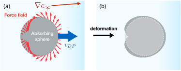
Fig.  19: : Local force acting on a diffusio-phoretic sphere. (a) Local force field acting on a sphere experiencing diffusio-phoresis with absorption at its surface in a solute gradient. The local force is plotted with an arbitrary factor amplitude factor (the same for each vector) and projected in the 2D plane; (b) Potential resulting deformation of the sphere, axisymmetric view, when the deformation is assumed to be proportional to the local force.

The situation is very different for electro-phoretic transport. As was first discussed in Ref.197, for electro-phoresis there is a local force balance between the direct electric force acting on the particle and the hydrodynamic shear acting on its surface: accordingly the local force simply vanishes identically. In physical terms, this is due to the fact that the electric force acting on the colloid particle exactly balances the electrical force acting on the electric double layer because of local electroneutrality (the charge in the electric double layer being exactly opposite to the surface charge). This can be actually verified explicitly by extending the previous calculations to electro-phoresis. This can be performed for weak electrostatic potential along the lines in Ref.¹⁹⁶, and it predicts indeed a vanishing local force.

Accordingly, particles undergoing electro-phoresis are not expected to deform, in contrast to diffusio-phoresis which leads to local deformations. Such results remain to be experimentally studied in order to observe the modification of a particle conformation undergoing diffusio-phoretic drift. We note however that in the context of thermo-phoresis, DNA was reported to stretch under a temperature gradient  ¹⁹⁸. Such effects could have interesting applications in the context of separation of particles, since their shape will differ depending on their size.

As a last comment, the previous discussion neglected surface transport at the surface of the particle: this involves convection of solute in the interfacial region, but also fluid slippage at the particle surface, which will both affect the steady-state concentration field of the solute around the particle. This leads to corrections to the mobility as a function of a (properly defined) Péclet number, as introduced in Refs.68, 69, 193, 199.

5.1.3 The diffusio-phoretic mobility

Let us now focus on the mobility. As for diffusio-osmosis, the diffusio-phoretic mobility scales as $\mu_{DP}\approx{\pm\,\lambda^{2}/\eta}$ where $\lambda$ is the thickness of the interfacial layer. For electrolytes, the latter identifies with the Debye layer thickness and one expects accordingly that $\mu_{DP}\sim 1/c_{s}$ so that one usually writes the diffusio-phoretic velocity under salt gradients as:

$$\bm{v}_{DP}=D_{DP}\bm{\nabla}\log c_{s}$$ (89)

The diffusio-phoretic mobility $D_{DP}$ has now the dimension of a diffusion coefficient. According to the previous estimates, one expects for electrolytes that $D_{DP}\approx k_{B}T/(8\pi\eta\ell_{B})$ with $\ell_{B}$ the Bjerrum length, so that the value for $D_{DP}$ is expected to be in the range – though slightly smaller – of diffusion coefficients of molecules (thus far larger than any colloid diffusion coefficient): experimentally typical values for $D_{DP}$ are in the range $D_{DP}\sim 0.1-1$ 10^-10m${}^{2}/$s ^{200, 78}. Note that, as for diffusio-osmosis, diffusio-phoresis under electrolyte gradients with unequal diffusion coefficients for the anions and cations ($D_{+}\neq D_{-}$) has an electro-phoretic contribution similar to Eq. (47) which can become quantitatively predominant; see also Ref.54. The expression in Eq. (89) highlights a “log-sensing” behavior, similar to that observed in bacteria, e.g. in E. coli ²⁰¹. It is at the basis of various unconventional transport phenomena which we discuss below.

Aside the case of electrolytes, other classes of relevant interactions involve steric exclusions – e.g. for neutral polymers – for which the mobility is expected to scale as $\mu_{DP}=R_{p}^{2}/\eta$ with $R_{p}$ the excluded particle diameter of the solute ^{54, 115, 202}.

On the experimental side, diffusio-phoresis has been investigated in numerous studies. First measurements were performed by the Russian school ⁵⁶, and later by Prieve, Anderson and collaborators in the 90’s ^{178, 179}. However the development of microfluidics over the last two decades has allowed to develop dedicated systems in which concentration gradients are perfectly controlled and tunable. It was then possible to measure diffusio-phoretic motion and obtain further insights into the phenomenon and its consequences ^{200, 77, 78, 203, 204, 21, 79, 205, 206, 207}.

While the above discussion assumed implicitly a dilute solute, the phenomenon is expected to occur under gradients of mixtures, and is denoted as solvo-phoresis ⁷⁹. This was for example investigated in a recent study by Paustian et al. ²¹, who showed that polystyrene colloids undergo motion in gradients of water-ethanol mixtures. The velocity of the particles was shown experimentally to obey

$$\bm{v}_{DP}=D_{DP}\bm{\nabla}\log X$$ (90)

where $X$ is the ethanol molar fraction, thus pointing to non-ideality effects. It would be interesting to disentangle the contribution of the dependence of the interfacial thickness with the molar fraction. As a final remark, a slightly different phenomenon is the so-called osmo-phoresis, which is obtained for permeable particles in which their interface plays the role of a semi-permeable membrane and reported in Ref.208.

5.2 Harnessing diffusio-phoresis: membrane less separation, log-sensing and localization

In this section we highlight a number of chosen examples to illustrate the impact and the applications of diffusio-phoresis in diverse physical situations. An interesting feature of diffusio-phoresis is that complex patterns of solute gradients can be rather easily achieved – in relative contrast to electric fields as driving forces – so that this phenomenon can induce particle motion in quite subtle ways leading to a wealth of counter-intuitive behaviors. Such solute patterns may occur naturally, for example due to evaporation leading then to drying film stratification ²⁰², in membrane fouling ²⁰⁷, or at dead-end pores, allowing for boosted extraction of particles in porous media ^{209, 210}, as well as in hydrothermal pores with steep pH gradients ¹⁸¹. Alternatively static or dynamic patterns of solutes can be designed thanks to dedicated microfluidic devices ^{78, 203}. An illuminating example was reported recently in Ref.182, showing that “chemical” beacons emitting solutes may allow to engineer ultra-long range nonequilibrium interactions between particles, up to millimeters – see Fig. 18-b.

Instead of being exhaustive, we discuss here several “elementary mechanisms”, which serve the purpose of highlighting the versatile manipulation of particle assemblies via diffusio-phoretic motion.

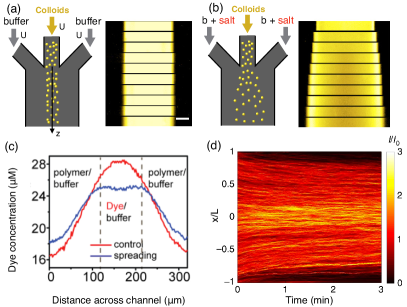
Fig.  20: : Harnessing diffusio-phoresis to transport particles. (a-b) Adapted from Ref.200. Fluorescent colloids are injected in the central branch of a microfluidic channel with three branches, with the same inlet velocity. They are imaged at different positions along the channel (side). In case (a) all channels have the same buffer composition (control), whereas in (b) salt (typically 10 mM of NaCl, LiCl or KCl) is added to the side channels. Although little dispersion is seen in case (a) due to the low diffusivity of colloids, a strong migration towards the high salinity is observed in (b). The horizontal scale bar is 50 $\mathrm{\mu}$m. (c) Dispersion of a dye (Rh6G, 50 $\mathrm{\mu}$M) at a cross-section of a microfluidic system with three branches similar to (a). The dye enters the central channel and the side channels are filled with polymer (5 wt % Ficoll 400K) for the spreading experiment (control, without polymer). Adapted from Ref.206 with permission from Springer Nature, copyright 2017. (d) Spatio-temporal evolution of particles upon exposure to CO₂ gradients (CO₂ is flown above and below, in $x=\pm L$). The particles are polystyrene, diameter $0.5\mathrm{\mu}$m, dispersed in a liquid buffer, and $L=400\mathrm{\mu}m$. Adapted from Ref.205, image under Creative Commons Attribution 4.0 International License.

Boosting migration – As a first example, we highlight how diffusio-phoretic transport leads to strongly enhanced migration of particles, with the fast solute “towing” the large, slow, particles. This effect was demonstrated in particular in coflow geometries, such as in Fig. 20, which was considered in various papers ^{200, 206, 205, 211}. This geometry is quite generic in microfluidics in the context of mixing and serves here the purpose of highlighting consequences of diffusio-phoretic motion. Colloids have a low diffusion constant and therefore barely mix in such a geometry, see Fig. 20-a. Adding tiny amounts of salt, typically millimolars, drastically boosts colloid dispersion – see Fig. 20-b-c – with an observed effective diffusion coefficient of the colloids which is 10 to 100 times larger than the equilibrium diffusion coefficient. As mentioned earlier, this is a consequence of diffusio-phoretic motion of the colloids under the salinity gradients present across the various parts of the channel. This can be rationalized on the basis of simple arguments. The growth rate for the width of the colloid suspension writes as $dw/dt=2v_{DP}=2D_{DP}\nabla\log c_{\rm s}$, with $c_{s}$ the inhomogeneous salt concentration. The latter relaxes via Fick’s diffusion and $\nabla\log c_{s}\approx\pm 1/\sqrt{D_{s}t}$ (the sign depending on the salt gradient direction), so that

$${dw\over dt}\approx\pm{2D_{DP}\over\sqrt{D_{s}\,t}}\,\,.$$ (91)

Note that in the experiments of Fig.20, the effective time is related to the position $z$ along the channel as $t=z/U$ ($U$ the average flow velocity). Integrating this equation yields immediately the observed diffusive like behavior,

$$w(t)-w_{0}=\pm\sqrt{2D_{\rm eff}t}.$$ (92)

with a diffusion coefficient $D_{\rm eff}\simeq{D_{\rm DP}^{2}/D_{\rm s}}$. Quantitatively $D_{\rm eff}$ is of the order of a (fraction of) salt coefficient $D_{s}$ so that $D_{\rm eff}\gg D_{0}$ (the colloid diffusion coefficient) and colloids “diffuse” much faster in the presence of (even minute) concentration gradients. Similar behaviors in equivalent geometries have been reported under CO₂ gradients ^{205, 211} or polymer gradients ²⁰⁶.

Localization – As a second example, diffusio-phoretic motion can be harnessed to manipulate and localize particle assemblies. Interestingly in the biological world, bacteria are capable of using solute contrasts to localize proteins ²¹². Localization is then used as an information for further vital processes, for instance localization of the ring of the FtsZ protein at midcell is used for cellular division ^{213, 214}. Similar features can be obtained on the basis of diffusio-phoresis under salt gradients, harnessing the log-sensing feature discussed above in Eq. (89), and leading to particle accumulation ^{77, 78}. Indeed, under a linear salt concentration gradient, the diffusio-osmotic velocity is not uniform and will be larger in regions of lower salt concentration – see Fig. 21-a. Alternating the gradient over time leads to rectification of diffusio-phoretic motion and accumulation of the colloids towards e.g.the center of the cell, as highlighted in Fig. 21-b. It is interesting on this elementary example to formalize the rectification process. The colloid and salt equations of transport obey the coupled Smoluchowski and diffusion equations

$$\partial_{t}\rho =-\bm{\nabla}\cdot\left(-D_{0}\bm{\nabla}\rho+D_{DP}\bm{\nabla}[\log c_{s}]\times\rho\right)$$ (93)

$$\partial_{t}c_{s} =D_{s}\bm{\nabla}^{2}c_{s}$$

with $\rho$ the colloid density and $c_{s}$ the salt concentration; $D_{0}$ and $D_{s}$ are the particle and salt diffusion constants and $D_{DP}$ the particle diffusio-phoretic mobility. Let us simplify the geometry to fix ideas and consider a one-dimensional channel. We consider an oscillating salt concentration profile, $\nabla c_{s}(x,t)=f(t)\Delta c_{s}/\ell$, with $\ell$ a characteristic length scale and $f(t)$ an oscillating function of time with zero average. Averaging over the rapid salt concentration oscillations, the mean diffusio-phoretic velocity which enters the Smoluchowski equation simplifies to $\bar{v}_{DP}=D_{DP}\langle\nabla[\log c_{s}]\rangle_{t}\approx-D_{DP}(\langle f^{2}\rangle_{t}/\ell^{2})\times x$, where $x$ is the distance to the center of the cell and $\langle\cdot\rangle_{t}$ an average over time. It can be rewritten in terms of an effective potential via

$$\bar{v}_{DP}\equiv\mu_{0}\times-\partial_{x}{\cal U}_{\rm eff},$$ (94)

with $\mu_{0}=D_{0}/k_{B}T$ the colloid mobility and

$${\cal U}_{\rm eff}(x)={k_{B}T\over 2}\langle f^{2}\rangle_{t}{x^{2}\over\sigma_{\ell}^{2}},$$ (95)

with $\sigma_{\ell}=\frac{\ell}{2}\sqrt{{D_{0}\over D_{DP}}}\ll\ell$. This illustrates that the rectified diffusio-phoresis of the colloids can be interpreted in terms of a harmonic trapping potential towards the central node ($x=0$) of the solute concentration oscillation pattern. This allows one to manipulate the colloidal population via time-dependent solute gradients.

Alternative routes for focusing colloidal populations were proposed using diffusio-phoretic transport without the requirement of time-dependent fields ⁸⁰ – see Fig. 21-c. These make use of combined steady gradients of salt and pH which are shown to yield localization of the particles. The interpretation of this subtle phenomenon incidentally highlights that the effects of gradients cannot be simply superimposed for diffusio-phoresis and a new formulation of coupled diffusio-phoretic transport was required, rewriting the driving solute gradients in terms of the corresponding ion fluxes. Such combination of gradients of pH and salts was suggested to occur in hydrothermal pores, with potential consequences on the emergence of an ion-gradient-driven early protometabolism and the origin of life ¹⁸¹. Finally focusing of colloidal particles was demonstrated in dead-end pore geometries ²¹⁰, with potential applications to preconcentration, separation, and sorting of particles.

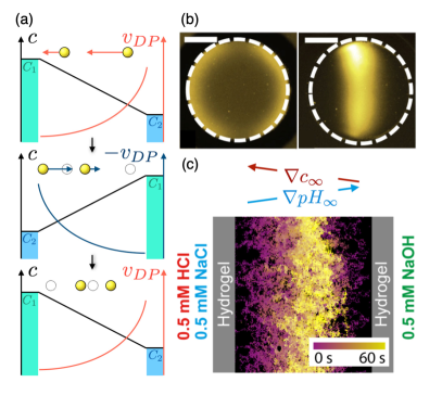
Fig.  21: : Focusing particles with diffusio-phoretic transport. (a) Trajectories of two (yellow) particles starting at different lateral positions upon an alternating concentration gradient. As the diffusio-phoretic velocity scales logarithmically with solute concentration, the particles closer to lower concentrations move faster, resulting in localization of the particles at the center. (b) Alternating fluids are flushed on both sides of a circular microfluidic well containing fluorescent colloids. The concentration of LiCl in the two side channels alternates (left/right) with period 480s, between buffer alone and 100 mM. The scale bar is 200 $\mu$m. (Left) Initial particle distribution in the well and (Right) stationary colloid distribution under the alternating concentration gradient. Reproduced from Ref.77. (c) Diffusio-phoresis under combined steady pH and salt gradients. Flowing NaOH and HCl solutions separately in two reservoir channels establishes a gradient in pH from 3.3 (left) to 10.7 (right), within which diffusio-phoretic particles proceed monotonically to the right. A NaCl gradient is superimposed on the pH gradient inducing diffusio-phoresis to the left. Streamline images reveal unexpected focusing at a location within the channel. Adapted from Ref.80 with permission from the APS copyright 2016.

Osmotic shock – As a last example, we discuss a very striking and counter-intuitive behavior steming from log-sensing, coined as osmotic shock, which was discussed in Ref.77. It illustrates that diffusio-phoresis keeps a long-lasting “memory” of solute gradients, even when they would be expected to be already homogenized. Consider a situation where the colloids are spread in a reservoir with lateral size $\ell$, with initially a uniform solute concentration $c_{0}$. Then at time $t=0$, solute is flushed at the boundaries, $c_{s}(x=\pm\ell/2,t)=0$ for $t>0$ (simplifying to 1D, and $x$ is the coordinate from the center of the reservoir). After a short transient, the solute concentration profile will decay to zero according to $c_{s}(x,t)\simeq c_{0}\exp[-t/\tau]\,\cos(\pi x/\ell)$, with $\tau=\ell^{2}/D_{s}$ the diffusion timescale of the solute. The diffusio-phoretic velocity of the colloids then writes $v_{DP}=D_{DP}\times\nabla\log c(x,t)$, so that

$$v_{DP}=D_{DP}\times{\pi\over\ell}\tan\left({\pi x\over\ell}\right)\approx D_{DP}\times{\pi^{2}\over\ell^{2}}\times x,$$ (96)

pointing towards the center of the reservoir, $x=0$, hence gathering the colloid population towards this position. From Eq. (96) it is clear that the DP velocity is therefore independent of time ! This leads to the counter-intuitive result that diffusio-phoretic motion occurs on far longer timescales than the solute diffusion timescale. This behavior was highlighted experimentally in Ref.77, where diffusio-phoretic motion of colloid particles was observed on timescales ten times longer than the naive diffusive timescale for the salt. Log-sensing is an efficient approach to localize colloids, but its application for trapping of other types of particles, e.g. polymers, remains to be explored. This could possibly be harnessed to improve sensors or traps for high throughput chemical reactions ²¹⁵. Applications to information storage and retrieval could also be explored ²¹⁶. Log-sensing also helps remove particles or fluids trapped in dead-end pores, as we will discuss in Sec.6.4.

As a final word on this section, the role of diffusio-phoretic transport in biological context has yet to be readily explored and quantified. In the toolbox of living systems, concentration gradients play a versatile role, readily exploited in many aspects of the biological machinery, such as energy reservoirs, but also serving more sophisticated functionalities, associated with spatial signaling, localization and pattern formation at the various scales involved in the biological processes. One may cite e.g. enzyme transport ²¹⁷, protein localization in bacteria ²¹² or more generally in spatial cell biology the use of concentration patterns for positional information ^{218, 219, 220}, to quote a few. Obviously chemotaxis in biological organisms under solute gradients is a highly complex phenomenon steming from the interplay of complex signalling pathways, quite far from the simple diffusio-phoretic transport discussed here. But one may reversely remark that the consequences of diffusio-phoresis as a physical phenomenon cannot be overlooked in biological materials, especially in the presence of ubiquitous gradients. This has been barely explored ²²¹.

5.3 From self-propulsion to self-assembly

Beyond the idea of passive diffusio-phoresis, where particles move under externally imposed solute gradients, arose the idea that the solute concentration gradients could be generated on the particle themselves, e.g. via chemical reactions occurring at their surfaces. For an asymmetric chemical reactivity, this self-diffusio-phoresis process thus generates self-propulsion of the particles, fueled by the chemical reactions ^{222, 192, 223}. Together with other phenomena leading to self-propulsion, this triggered the emergence of the field of active matter, which has exploded over the last decade. It is not our purpose to review this field, as this goes beyond the scope of our focus on osmotic forces and we refer to some recent reviews on this topic ^{224, 223, 225}. We however highlight here a few phenomena where osmosis, via diffusio-phoresis and related mechanisms, is explicitly at play.

Self-diffusio-phoresis – On the experimental side, the phenomenon of self-diffusio-phoresis was pioneered by Paxton and coworkers ²²⁶, who showed self propulsion of Platinum/Gold nanorods in hydrogen peroxide. Hydrogen peroxide is chemically transformed differentially on both metals, either forming or being depleted on each side of the rod, and this creates a gradient of the reacting specie (here hydrogen peroxide) driving diffusio-phoresis, see Fig. 22. For such bimetallic particles with redox reactions on both sides of the particle, self-electro-phoresis may actually contribute to the driving force, via motion of charges (electrons and ions) within and outside the particle. Self-diffusio-phoresis was further demonstrated in colloidal janus particles of various materials, see Refs.227, 228, 229, 230, 231, 232, 233, 234, 235, 236, and Refs.224, 237 for a more exhaustive literature on this aspect.

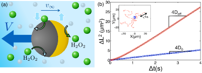
Fig.  22: : Self-propelled particles. (a) Chemical reactions occur differentially at the front and at the rear of a reactive colloidal particle, thereby inducing a chemical concentration gradient. This leads to diffusio-osmotic driving at the surface, hereby displacing the particle. (b) Experimental mean squared displacements $\Delta L^{2}(\Delta t)$ and 2D trajectories (inset) for bare (blue) and active colloids (red) in 7.5$\%$ H₂O₂ solution. Bare colloids (bottom) show standard diffusion ($\Delta L^{2}$ linear in time), while the mean squared displacement of active colloids shows a ballistic motion at small timescales and a diffusive motion at longer timescales. The measured diffusion coefficients are $D_{0}=0.33\mu$m${}^{2}/$s for bare and $D_{\rm eff}=1.9\mu$m${}^{2}/$s for active colloids. Reproduced from Ref.229 with permission from the APS, copyright 2010.

On the theoretical side, the mechanisms by which the creation or removal of species on the particle’s surface generate an osmotic pressure gradient and motion are not obvious and there has been some initial debate on this question, see Refs.186, 188, 190, 187, 189. This echoes directly our discussion about the diffusio-phoretic force balance in Sec. 5.1.2. Actually the question was pioneered by Lammert et al. on the putative self-electro-phoresis of biological cells or vesicles driven by non-uniform ion pumping across the bounding membrane ²³⁸. Echoing this situation, an illuminating model for self-propulsion via asymmetric osmotic driving force was introduced by Golestanian et al. ^{239, 111}. They considered a particle exhibiting a non-uniform chemical reactivity on its surface, as defined by the corresponding solute flux on its surface $\alpha(\bm{r})=-D_{r}\nabla_{\perp}C_{\rm react}$ (corresponding to the generation or consumption of the solute by the chemical reaction), $D_{r}$ being the diffusion constant of the reactant. This boundary term is coupled to the diffusive dynamics of the solute concentration in the bulk. The resulting concentration gradient induces a diffusio-osmotic slip velocity $v_{DO}$ at the surface, depending on the position, and accordingly particle motion. In the case of a janus sphere, exhibiting a contrasting chemical reactivity on its two moieties, the self-diffusio-phoretic velocity $V$ takes the simple expression

$$V=\langle v_{DO}\rangle_{sphere}={1\over 8D_{r}}(\alpha_{-}-\alpha_{+})(\mu_{+}+\mu_{-})$$ (97)

where $\alpha_{\pm}$ is the chemical reactivity on the two sides and $\mu_{\pm}$ the local surface phoretic mobility. We emphasize though that on the experimental side, other mechanisms also contribute to the motion of catalytically self-propelled particles, like self-electro-phoresis ¹⁹².

To some extent, such "active particles" mimick self-propelled biological organisms. The possibility to fabricate artificially these systems constitutes a playground to study far-from-equilibrium behaviors ²²⁴. Because active particles consume energy at a local scale, their collective behavior is a priori not constrained – at least to some extent – by thermodynamics and may possibly allow to break the bottleneck of the second principle; cf. the beautiful example of the rotating Feynman ratchet with active materials in Ref.240.

Active suspensions – Such active particles have fascinating behaviors, and we focus on a few examples. First, self propulsion leads to ballistic motion on short timescales, but orientational random motion leads to diffusive behavior on long timescales, in a way similar to the so-called “run and tumble” motion of bacteria. The effective diffusion coefficient is however far larger than the bare diffusion coefficient based on the Stokes-Einstein estimates $D_{0}$ ^{228, 229}, see Fig. 22-b. As a rule of thumb the effective diffusion coefficient is typically $D_{\rm eff}\approx V^{2}\times\tau_{R}$, where $V$ is the self-propelling velocity and $\tau_{R}$ is the timescale for rotational brownian motion: $\tau_{R}\sim D_{\rm rot}^{-1}\sim R^{2}/D_{0}$, where $D_{\rm rot}$ is the rotational diffusion coefficient, $R$ the particle size. As a consequence the particles behave as a “hot” bath, with a high effective temperature defined from a “fluctuation-dissipation”-like relation as ${k_{B}T_{\rm eff}}=D_{\rm eff}/\mu_{0}$, where $\mu_{0}=D_{0}/k_{B}T$ the bare particle mobility, so that

$${k_{B}T_{\rm eff}}\approx k_{B}T\times{V^{2}\,\tau_{R}\over D_{0}}$$ (98)

(up to numerical prefactors). Altogether this predicts that $T_{\rm eff}/T\sim Pe^{2}$ where the Péclet number is defined in terms of the self-phoretic velocity as $Pe=V\,R/D_{0}$. This prediction was further confirmed experimentally²²⁹.

Osmotic pressure of active suspensions – The question of the osmotic pressure created by active particles was raised in a number of theoretical and experimental works ^{241, 242, 243, 234, 244}. As we introduced above, the osmotic pressure acting on the fluid can be defined mechanically via the average force exerted by the active particles on a semi-permeable wall. In the case where the active particles exhibit a Boltzmann-like equilibrium in the presence of the wall (say, represented by an external potential), as shown e.g. for sedimentation profiles ²²⁹, then the osmotic pressure reduces to the van ’t Hoff law, except that the temperature is replaced by the effective temperature of the suspension:

$$\Delta\Pi\simeq k_{B}T_{\rm eff}\times\Delta\rho$$ (99)

where $\rho$ is here the concentration of active particles, and the effective temperature $T_{\rm eff}$ was introduced above. This matches the equation of state measured using sedimentation profiles ²³⁴.

However Boltzmann-like equilibrium is expected to fail in some limiting situations for active particles. In particular it is commonly observed that self-propelled particles do hit “compulsively” hard surfaces, similarly to a fly on a window ²⁴⁰: in such cases, the particle remains stuck at the membrane’s surface until it reorients, and there is a non-boltzmannian accumulation of particles at the membrane. This is nicely exemplified in the run-and-tumble model under an external field, where strong deviations from the Boltzmann profile is predicted when the typical drift velocity $V_{d}=\mu_{0}{\cal F}_{\rm ext}$ (with ${\cal F}_{\rm ext}$ the maximum external force, say, due to the separating membrane), is larger than the particle self-propulsion speed $V$ ²⁴⁵. This situation occurs for steep potentials. When such accumulation occurs, the corresponding osmotic push will differ from the simple van ’t Hoff law, see Refs.243, 244. In particular, the osmotic pressure depends on the properties of the membrane itself and its interaction with the particles – typically via the ratio between the typical membrane characteristic steepness and the particle mean-free path ²⁴⁴ –, in strong contrast to the van ’t Hoff “universal” relation. Similar deviations from the van ’t Hoff law also occurs when the interaction between the active particles and the membrane involves wall-induced rotational torques ²⁴².

Towards self-organization and self-assembly – Another interesting feature of particles propelling via self-diffusio-phoresis is that they interact via chemical signaling. Propelled particles act as a beacon – similarly to the situation considered in Ref.182 – and leave a “trace” of their passage in the form of a diffusing cloud of chemicals which will be felt by other paticles, see Fig. 23. Accordingly other active particles will be reoriented towards or against ^{246, 247} the active particle via diffusio-phoretic motion (on top of their self-driving motion). Indeed the surface creation or consumption of solutes generates long-distance distortion of the solute concentration profile, typically relaxing spatially as a monopole $\delta c_{s}\sim 1/r$ (the scaling deriving from Fick’s equation with a sink). This long-range interaction is for example highlighted in Fig. 23-b, showing the diffusio-phoretic attractive motion induced by a single beacon, from Ref.231. At shorter range, the interaction may become more complex and requires detailed investigation of the chemical drivings ²⁴⁷.

This osmotic-induced chemical interaction is at the origin of many advanced collective properties of active particles, such as clustering ^{230, 232, 224, 248}, or self-assembly ^{231, 235}, see Fig. 23-c-d. Out-of-equilibrium self-assembly has raised enormous interest, since activity leads to unexpected structures, with the hope of designing novel and smart materials ²²⁴.

It is interesting to formalize the basics of the phenomenon at stake by writing the coupled diffusion-reaction equation for the colloid population and solute concentration. For the purpose of illustration, we only consider here a single neutral chemically generated specie which acts as a chemo-attractant to the colloids. These dynamical equations actually identify with the so-called Keller-Segel equation, which were written to describe the chemotactic aggregation of a slime mold (amoebae) under the perspective of a dynamical instability ^{249, 250, 230}:

$$\begin{split}\partial_{t}\rho&=-\bm{\nabla}.\left(-D_{\rm eff}\bm{\nabla}\rho+\mu_{DP}\bm{\nabla}c_{s}\times\rho)\right)\\ \partial_{t}c_{s}&=D_{s}\bm{\nabla}^{2}c_{s}+\alpha\rho\simeq 0\end{split}$$ (100)

with $D_{\rm eff}$ the effective diffusion coefficient of the active colloids, $D_{s}$ the diffusion coefficient of the “chemo-attractant” specie and $\alpha$ the chemical rate of the powering chemical reaction occurring at the surface of each colloid; we assume here that the solute dynamics are fast. By analogy to electrostatics, the second equation for the solute allows one to obtain the solute concentration as a function of the colloid density, as $c_{s}(\bm{r})\simeq{\alpha/D_{s}}\int d\bm{r^{\prime}}\,\rho(\bm{r^{\prime}})/4\pi|\bm{r}-\bm{r^{\prime}}|$. When introduced in the first equation in Eq. (100), this shows that the diffusio-phoretic attraction acts as a self-consistent effective potential such that

$${\cal U}_{\rm eff}(\bm{r},\{\rho\})=-{\mu_{DP}\over\mu_{0}}\,{\alpha\over D_{s}}\int d\bm{r^{\prime}}\,{\rho(\bm{r^{\prime}})\over 4\pi|\bm{r}-\bm{r^{\prime}}|}.$$ (101)

with $\mu_{0}$ the bare colloid mobility. Equivalently, the dynamics of the colloid population can be formally derived from an effective free energy functional of the colloid system which takes the simple form

$${\cal F}_{\rm eff}= k_{B}T_{\rm eff}\int d\bm{r}\left[\rho(\bm{r})\log\rho(\bm{r})-\rho(\bm{r})\right]$$ (102)

$$-{1\over 2}\left({\mu_{DP}\over\mu_{0}}\,{\alpha\over D_{s}}\right)\int d\bm{r^{\prime}}d\bm{r^{\prime\prime}}\,{\rho(\bm{r^{\prime}})\,\rho(\bm{r^{\prime\prime}})\over 4\pi|\bm{r^{\prime}}-\bm{r^{\prime\prime}}|}$$

This highlights that the “osmotic interaction” via the diffusio-phoretic motion induced by the solute traces leads to long range non-equilibrium interactions. This is expected to lead to strong collective effects, such as the clusterization observed experimentally. For attractive systems, $\mu_{DP}>0$, these equations are formally analogous to a (non-inertial) gravitational system. Keller-Segel and subsequent works have shown that the above equations predicts an aggregation mechanism, similar to a Chandrasekhar gravitational collapse ^{249, 250}. Similar conclusions were predicted for thermally active colloids ²⁵¹ where the threshold for collapse was rederived.

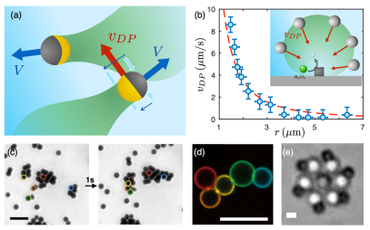
Fig.  23: : Out-of-equilibrium self-assembly. (a) Sketch of the diffusing chemical trace left behind active particles, and which modifies the local chemical gradient. Another active particle approaching this chemical gradient will therefore sense a different driving velocity along its edge, changing its trajectory (here in an attractive configuration) (b) Courtesy from Jeremie Palacci, data from Ref.231. Passive colloid diffusio-phoretic speed as a function of the distance to a hematite cube that can be used – with blue light – to catalyse the dissociation of H₂O₂. (c) Spontaneous self-assembly of active particles. The particles form various cluster sizes and shapes. The scale bar is 10$\mu$m. Reproduced from Ref.230 with permission from the APS, copyright 2012. (d) Sequential self-assembly of DNA-grafted droplets, the different colors represent different functionalizations. The scale bar is 10$\mu$m. Reproduced from Ref.252, image under Creative Commons Attribution 4.0 International License. (e) Targeted assembly of phototactic swimmers into nanogears. The scale bar is 1$\mu$m. Reproduced from Ref.235 with permission from Springer Nature, copyright 2018.

However the clusters observed in the experiments, e.g. in Refs.230, 231, 248, do not correspond to full collapse and are rather dynamic, with clusters reaching a finite size and continuously rearranging over time, see Fig. 23-c. As shown in Refs.253, 254, this behavior can be reproduced by Keller-Segel-like dynamics provided both translational and rotational phoretic conditions are properly taken into account in the kinetics. Using this framework, it is furthermore possible to predict the condition in which dynamic clusterization occurs ^{253, 254}, in good agreement with the experiments.

Beyond clusterization, the self-diffusio-phoretic motion of particles and their osmotic interactions were shown lately to lead to the self-assembly of active particles into higher levels of structure organization. This is highlighted in Fig. 23-e, from Ref.235, where self-spinning microgears are built on the basis of these non-equilibrium interactions. Beyond, more "on demand" structures are possible, like structures assembled through DNA-grafted interfaces ^{255, 252, 256} (see Fig. 23-d).

6 Osmosis, towards applications

From food processing in biological organisms ^{257, 258, 259}, to reverse osmosis for desalination and energy generation from salinity differences ^{31, 260, 73, 261}, osmotic forces are harvested in a considerable number of applications in very different domains. In this section we review more specifically a variety of such applications based on (recently) elucidated transport mechanisms relying on osmotic forces.

6.1 Water treatment and membrane separation

6.1.1 Reverse and forward osmosis and their limitations

Access to clean water and cleaning water from industrial waste is a great challenge²⁶²: in 2015 still 663 million people worldwide lacked access to drinkable water ²⁶³, and cleaning waste water is becoming a major challenge in oil and gas industries ^{264, 265}; going further, some new regulations may appear to enforce a zero liquid discharge for industrial waste, thus requiring complete recycling of water ressources ²⁶⁶. On a day-to-day basis, humanity consumes the equivalent of 10-100 cubic kilometers of fresh water ²⁶⁷ for all purposes (agriculture, industry, domestic). Because fresh water is not directly accessible everywhere, and in order to cover the growing need for freshwater, desalination of sea water and cleaning of waste water have become essential.

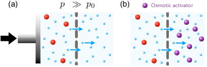
Fig.  24: : Reverse Osmosis and Forward Osmosis. (a) Schematic explaining reverse osmosis, occurring via a piston applying a large hydrostatic pressure $p$ such that the difference to the atmospheric pressure (pressure of the other compartment) is larger than the osmotic pressure $p-p_{0}\geq\Delta\Pi$. (b) Schematic explaining forward osmosis, occurring via the addition of some soluble species (here the purple solute) that increases the osmotic pressure on the drought side and therefore "attracts" water from the brine side.

Lately, membrane based technology has established itself for water purification. Reverse osmosis is the most broadly used technique (representing 62-65$\%$ of the installed capacity in 2015 for desalination ^{268, 269}, 24$\%$ being thermal based technologies). Reverse osmosis relies on the very simple principle of applying an external large hydrostatic pressure to counterbalance the osmotic pressure difference and induce a flow of water towards the low concentration side – see Fig. 24-a. In particular, one can therefore extract water from seawater by concentrating seawater even more, or extract water from waste water (in a simplistic view). For desalination the pressures involved are typically of 30-50 bars in order to exceed the osmotic pressure.

In a different approach, forward osmosis (combined with thermal methods for desalination) makes use of draw solutions to counterbalance the salinity induced osmotic pressure ^{270, 271, 272} – see Fig. 24-b. Generating a high osmotic pressure, typically above the 30 bars of pressure between sea and fresh water, requires draw solutes which are highly soluble in water, and also with a sufficiently small size (hence low molecular weight). Indeed, as a rule of thumb, for a solute with elementary volume ${v}_{0}\sim r^{3}$ with $r$ the solute size, the maximum osmotic pressure which can be achieved is typically $\Delta\Pi\sim{k_{B}T\over v_{0}}$. This would suggest that solutes with size above $1$ nm are not able to achieve a sufficiently high osmotic pressure for desalination (note that this argument forgets departures from ideality, which could increase more strongly the osmotic pressure). In a more subtle way, a solute with a strong affinity towards water may also decrease the water chemical potential and modify accordingly the pressure. This echoes the huge pressure drops measured with hydrogel structures ²⁷³.

A number of other membrane based techniques with similar geometry are used or being developed, from electrodialysis (based on electric potential driving of salts) ^{274, 275} to capacitive deionization ^{276, 277, 278}, but also shock electrodialysis based on the idea of combining salt recovery with a porous charged material ²⁷⁹, concentration polarization  ²⁸⁰, and other techniques harnessing chemical phenomena like adsorption desalination ²⁸¹ or biodesalination ^{282, 283} and bio-water treatment ²⁸⁴.

Membrane-based technologies suffer from a number of limitations. First, they have a high-propensity to fouling by molecules which are larger than the critical molecule size allowed to pass ²⁸⁵; also due to the large pressures applied during reverse osmosis. Second, because they are passive membranes – essentially discriminating particles upon their size – they can not be at the same time very selective and highly permeable. This was formalized for ultrafiltration membranes in Refs.286, 287. In fact increasing the permeability of a membrane (and therefore the energy required to recover a given amount of cleaned water) requires essentially to broaden the size of the pores, as water flow within pores is limited by friction on the pore walls. However this leads inevitably to a decrease in the selectivity or separation properties of the membrane; and reciprocally. This is called the selectivity-permeability trade-off. For nanofiltration membranes (used for reverse osmosis and so on) the same trade-off exists although the proper establishment of a limiting regime is still empirical ²⁶¹ – see Fig. 25. Finally, one challenging progress route for membrane separation is the ability to perform molecular scale design ²⁸⁸ and therefore to ensure the best selectivity properties to eliminate e.g. micropollutants, some of which are of great concern for health ²⁸⁹. Overall, it should be realized that the main current challenge in desalination and water purification is not really the permeability of the membrane, but rather achieving a well-controlled selectivity to retain/reject specific species.

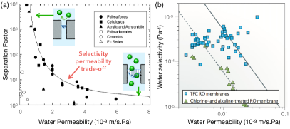
Fig.  25: : Selectivity Permeability Trade-off. (a) Adapted from Ref.286. Selectivity versus permeability values for ultrafiltration membranes (used for separation of larger molecules than salt ions). Bovine serum albumine is the model molecule for selectivity. The line indicates the standard selectivity permeability model (with a log normal distribution of pores, Poiseuille flow and selectivity given by Zeman and Wales exclusion rules ²⁹⁰). (b) Adapted from Ref.261 with permission from Springer Nature, copyright 2016. Selectivity versus permeability values for reverse osmosis membranes using salt as the model specie for selectivity. The lines correspond to the empirical models inspired from Ref.291 to relate maximal selectivity and permeability in reverse osmosis membranes.

6.1.2 What can we expect from new nanomaterials and nanofluidic devices ?

It may appear that developing the “ideal membrane”, which is both highly selective and highly permeable, is like squaring the circle. However, Nature has achieved this tour-de-force, with water porins like aquaporins exhibiting unrivalled performances in terms of selectivity and permeability ²⁹². This requires to develop new artificial materials with properly decorated nanopores allowing for such exquisite design, for example self-assembled artificial water channels ^{292, 293, 294}, or tailor-made DNA origami channels ^{86, 150}. This is actually a challenge that nanoscale science may be up to ^{152, 88, 292, 295}.

The development of new nanomaterials has indeed allowed the emergence of new avenues for membrane separation. Graphitic materials of various forms and geometries, such as carbon nanotubes, graphene and lately graphene oxides membranes, have raised considerable promises, see Refs.152, 88 for reviews on this topic. Carbon materials were consistently shown to exhibit ultra-low water friction and high permeability, and this represents a key asset to minimize the viscous loss in separation processes. Furthermore advanced functionalization allows one to decorate the nanotubes improving selectivity ^{72, 296, 297}. Membranes made of nanopores in e.g. 2D graphene sheets have a molecular thickness, while keeping high mechanical strength: this accordingly increases the driving forces for transport (which scale like the inverse thickness) by orders of magnitude, hence all transport coefficients and the overall efficiency of the process ⁸⁸.

Still, these graphitic systems – carbon nanotubes, graphene slits and more generally 2D materials – remain difficult to fabricate as large-scale membranes. Upscaling towards industrial applications is a considerable challenge. The advent of graphene oxide membranes and their derivatives may change the story. These are constituted of graphene flakes, which organize into parallel stacks of graphene layers, having nanoslits in a staggered alignment and an interlayer distance which is typically below the nanometer. In spite of the complex labyrinthine flow across multiple graphene layers ²⁹⁸, the membranes demonstrate large permeability ^{299, 300}. Last but not least, they are relatively easy to fabricate at large scale. Such systems therefore appear as ideal membranes for ionic separation ³⁰¹ and may well revolutionize the domain of filtration.

Now, beyond materials themselves, it should be realized that nanoscales allow for many new “exotic” transport phenomena, the consequences of which have – up to now – been barely harnessed. One may quote for example the membranes made of hydrophobic nanopores, making use of nanobubbles as a semipermeable sieve for osmotic phenomena ¹⁴⁹; or the ionic and osmotic diodes, allowing for rectified transport in membranes, or the active osmotic phenomenon, as we discussed above; or in a different context, the specific adsorption properties of graphene oxide membranes allowing for water-ethanol separation in membranes³⁰², which are far more efficient than standard distillation. Such routes would deserve a proper exploration to go beyond the relatively basic sieving principles underlying membrane science. These should offer alternative routes for filtration and separation which still need to be invented.

6.2 Osmosis in biological systems: aquaporins, ion pumps and the kidney

Osmotic forces are harvested in the biological world in a considerable variety of phenomena and contexts: to store energy, induce mechanical motion, control ejection and absorption of compounds, etc. Osmotic pressure was much studied at first in plants ⁵, and one may in fact assess that plant life depends on osmotic forces. Indeed plants can not rely on muscle for force generation, yet they are able to achieve tensile and compressive stresses on a much wider range ³⁰³. To produce motion or growth, they rely on an underlying hydraulic machinery driven by osmotic or humidity gradients. For example, phloem  flow harnesses osmotic driving to transport sugar over long distances ^{304, 305, 258, 306, 259}. Osmotic transport is critical to regulate size in e.g. conifer leaf ³⁰⁷. The opening and closing of stomata on leaves  ³⁰⁸ and the circadian motion of various plants and flowers ^{309, 310} is regulated by swelling or shrinking driven by water flows. Those flows are generally actuated by active transport of solutes through specialized pumps ^{311, 312}. Even biofilms harvest osmotic pressure gradients in the extracellular space for surface motility ³¹³.

In animals and human beings, a number of processes involve osmotic flows for water or volume regulation and transport: from the kidney ³¹⁴ to the liver ³¹⁵ and the intestine ³¹⁶, not forgetting salivary secretion ³¹⁷. Cells harvest osmotic forces in a variety of ways, most obviously to control expansion and regulate size, e.g. in cysts ³¹⁸, and also to regulate absorption ³¹⁹ or ejection of genetic material ³²⁰ via small capsules. A number of processes also harvest more subtle forces in a fascinating way and we cite a few to engage the curious reader. Osmotic pressure changes may affect frequency of miniature end-plate potentials in neuromuscular junctions ^{321, 322}, but also drive oscillatory flows for cell regeneration ³²³. Electro-osmosis is harvested for uphill transport of water by insects in draught areas ³²⁴ but also more generally for epithelial transport ^{325, 326}.

The list of examples of osmotic transport in biological systems is nearly infinite, and occurs at all possible scales from individual molecules to organs and tissues. It is pointless to attempt a thorough review. Rather, we discuss below in more detail three specific biological phenomena related to osmosis. These examples raise in particular the question of whether such phenomena may be mimicked artificially to achieve advanced osmotic transport in artificial devices.

6.2.1 Aquaporins: the ideal semi-permeable membrane

A decisive turnpoint in the study of nanoscale systems was triggered notably by the discovery of nanoscale channels in biology. One of the most famous of these channel families is the aquaporin family (the most common being AQP1 or CHIP-28, see Fig. 26-a) ^{327, 328}. An aquaporin is a water-specific channel; aquaporins are present in many organs in living systems, animals, but also plants ³²⁹: they play a central role in the human kidney (see below), are also key role players in red blood cells and many other organs ³³⁰, and regulate water uptake in plants ³³¹. The striking specificity of aquaporins is that they are both highly selective to water and highly permeable. The permeability of an aquaporin was measured notably by P. Agre et al. to be in the range of $p_{f}=11.7\times 10^{14}$ cm³.s^-1 at 37^∘ C ^{332, 333} (with $p_{f}$ here defined as $Q=p_{f}\,v_{w}{\Delta p}/k_{B}T$; $Q$ is the water flux and $v_{w}$ the bulk water molecular volume). This corresponds to $\approx 3$ million water molecules translocating per second per bar ($p_{f}$ being related to the particle flux $dN/dt$ according to $dN/dt=({p_{f}/k_{B}T})\Delta p$). The value of the permeability of the aquaporin is much larger than that for other channels, see ²⁹² for a comparison, or what would predicted by continuum dynamics at these scales ^{335, 62}.

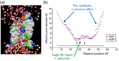
Fig.  26: : The aquaporin AQP1 water channel. (a) Molecular dynamics simulation of water transversing an aquaporin channel. Snapshot from movie in Ref.336 under Creative Commons license, in complement to Ref.337. (b) Effective pore diameter of the AQP1 and GlpF channels. Pore diameters were determined with AMBER-based van der Waals radii and analysed using the program HOLE38. Reproduced and adapted from Ref.338 with permission from Springer Nature, copyright 2001.

Aquaporins present several intriguing features: surprisingly they are hydrophobic channels ³³⁸ and they are extremely constricted ³³⁸ – only 3 Å in diameter at the narrowest point that allows for this selectivity. An aquaporin-based membrane constitutes therefore a somewhat ideal semipermeable membrane. All of its exceptional transport properties are intimately connected to its nanoscale (and even Ȧngström-scale) structure – thus hinting to the striking and appealing properties of fluid flow at the nanoscale. It is thus natural to look for artificial solutions for semi-permeable membranes harvesting properly designed nanoscale structures ^{293, 294}. For example, aquaporins present a sophisticated hourglass shape, that is believed to enhance the water permeability ³³⁹, see Fig. 26-b. Such a geometry could be readily mimicked using e.g. pore coatings ³⁴⁰ to enhance permeability of membranes.

6.2.2 Kidney: an ultra-efficient and unconventional osmotic exchanger

As a second example, we discuss the separation process occurring in the kidneys. As we highlight, the efficiency of the kidney filtration process takes its root in a very unconventional osmotic process, and could be inspirational for future separation technologies.

Per day, the human kidney is capable of recycling about 200 L of water and 1.5 kg of salt, separating urea from water and salt at the low cost of 0.5 kJ/L ³⁴¹ while readsorbing $\simeq$ 99$\%$ of the water input. The core of the kidney separation process lies in the millions of parallel filtration substructures called nephrons ³⁴¹. A striking feature is that the nephrons of all mammals present a precise loop geometry, the so-called Loop of Henle - in the shape of the letter "U" – see Fig. 27-a. This loop plays a key role in the urinary concentrating mechanism and has been extensively studied from a biological and physiological point of view ^{341, 342, 343, 344, 345}.

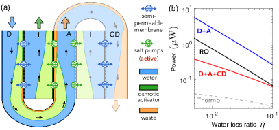
Fig.  27: : The osmotic exchanger principle of the kidney. (a) Inspired from Ref.314. Water, salt and urea molar fractions are represented in various colors along the U tube (descending, D and ascending A) limbs and the interstitium (I). For visibility, the water molar fraction was divided by 100. Black arrows represent the direction of flow. A semi-permeable membrane (containing aquaporins) separates the descending limb and the interstitium, while the ascending limb contains salt pumps transporting actively the salt to the interstitium. A third limb, the collecting duct (CD, in lighter collers) also exchanges with the interstitium via a semi-permeable membrane. The latter is crucial for the overall efficiency of the separation process. (b) Adapted from Ref.314. Power required for the functioning of the separation process as a function of the targeted water loss ratio: for the simple loop geometry (A+D), for the full serpentine (A+D+CD), as compared to the equivalent reverse osmosis process under a pressure gradient (RO). (a) and (b) are under Creative Commons Attribution 3.0 License.

As put forward in Ref.314, the U loop acts as an osmotic exchanger, similar in concept to a thermal exchanger – see Fig. 27-a. A mixture of water, salt and urea (or any other compound to be separated) enters and flows through the tubular U loop. Water and ions may be exchanged through the tube walls with a common interconnecting media, called the interstitium. On the descending side (D), aquaporins allow for water permeation across the walls. On the ascending side (A), salt is actively pumped, using an external source of energy (in the case of the kidneys, the dissociation energy of Adenosine Tri-Phosphate, ATP). This pumped salt results in an increased salt concentration in the interstitium, higher than the concentration of salt and urea in the descending tube (D). The osmotic pressure is therefore inverted and drives water from the U tube to the interstitium across the aquaporin channels. As a result, urea is highly concentrated in the U loop, while salt and water are redirected from the interstitium towards the blood circulatory network. This U-shape geometrical design is key to the efficient operation of the separation. Note that the third limb following the U-tube plays a crucial role in enhancing the separation efficiency ³¹⁴.

One may actually estimate the working efficiency of this osmotic exchanger in a simple way, providing a lower bound on the separation ratio. It is quantified in terms of the amount of lost water $\eta=c_{w}^{\rm A,top}v_{\rm A,top}/c_{w}^{\rm D,top}v_{\rm D,top}$, where $v$ is the flow velocity calculated at the top of the ascending (A) or descending (D) branch, and $c_{w}$ is the concentration of water. For the system to work, water has to flow from the descending branch towards the interstitium and this requires that chemical activities obey $a_{\rm D,top}^{\rm Water}\geq a_{\rm I,top}^{\rm Water}$. The latter can be expressed simply (in the low concentration regime) in terms of molar fractions and one obtains

$$\frac{c_{w}^{\rm D,top}}{c_{w}^{\rm D,top}+c_{s}^{\rm D,top}+c_{\rm waste}^{\rm D,top}}\geq\frac{c_{w}^{\rm I,top}}{c_{w}^{\rm I,top}+c_{s}^{\rm I,top}}$$ (103)

where $c_{w}$, $c_{s}$ and $c_{\rm waste}$ are respectively the concentrations of water, osmotic activator (salt) and waste. Assuming that all the osmotic activator has been reabsorbed in the upper branch yields $c_{s}^{\rm I,top}=\frac{v_{\rm D,top}}{v_{\rm I,top}}c_{s}^{\rm D,top}$. Water flow is conserved and thus $c_{w}^{\rm D,top}v_{\rm D,top}=c_{w}^{\rm I,top}v_{\rm I,top}+c_{w}^{\rm A,top}v_{\rm A,top}$. A lower bound for the fraction of lost water $\eta_{\rm lost}$ can then be simply deduced from Eq. (103) as

$$\eta_{\rm lost}\geq\left(\frac{c_{\rm waste}^{\rm D,top}}{c_{s}^{\rm D,top}+c_{\rm waste}^{\rm D,top}}\right)^{n}.$$ (104)

with $n=1$. For the geometry including a third reabsorbing branch, the collecting duct, see Fig. 27-a, a similar reasoning yields the same result with $n=2$. The square exponent thus leads to much smaller lost water fraction $\eta_{\rm lost}$ showing that this third branch is essential in the overall efficiency of the kidney separation. Using physiological values for the concentration, this estimate provides a prediction for water reabsorption, and thus urea separation, in the range of $\eta_{\rm lost}\sim 1$%, which is in excellent agreement with every-day life experience; see 314. To some extent, note that the osmotic exchanger of the kidney may be compared to a forward osmosis process. However the key difference is the geometry with 3 limbs that allows for a more efficient reabsorption of water.

In fact, energy wise, this system is also shown to be far more efficient than standard reverse osmosis principles, as can be estimated within the above model, see Fig. 27-b. In living systems, the nephron operates the separation of urea from water near the thermodynamic limit, $\simeq$ 0.2 kJ/L ³¹⁴. Yet, standard dialytic filtration systems, which are based on reverse osmosis and passive equilibration with a dialysate, require more than two orders of magnitude more energy ³⁴⁶.

Some attemps to build artificial devices mimicking the nephron were reported in the literature, but they rely on biological tissues or cell mediated transport, and cannot be easily scaled up and transferred to other separation devices ^{347, 348, 349}. None of the approaches so far rely on the specific geometry of the U-loop to improve the filtration process. Mimicking the separation process occurring in the kidney based on the physical perspective described above can now be foreseen using microfluidic elementary building blocks. Such an artificial counterpart could have definite impact in improving the early stage of desalination processes consisting in water pre-treatment to suppress large polluting molecules, and, down-the-road, could lead to substantial progress in dialysis for patients suffering from kidney failure.

6.2.3 Proton pumps, chemi-osmosis and advanced ionic machinery

As a last example, we discuss proton pumps and channels, which are compelling illustrations of how Nature harvests osmotic forces to drive mechanical parts. Biological systems have developed a fascinating artillery of devices to passively and actively transport ions, namely ionic channels and ion pumps. Among these, proton pumps are canonical examples. We detail a few examples below.

Proton pumps to build proton gradients – There exists a great variety of ways to actively transport protons in biology, from combined proton-electron transfer in cytochrome oxidase (crucial for respiration ³⁵⁰) to proton pumps implying the participation of ATP – the latter are called H⁺-ATPases ³⁵¹. ATP-ases play a key role in bio-energetics and are ubiquitous in many forms of life and plants ³⁵². They include three types. The P-type ATP-ases include in particular the plasma membrane H⁺-ATPase, that uses the dissociation energy of ATP to form gradients of protons. These gradients are crucial for plant movement (from phloem loading, to size regulation in the stomatal aperture, to tip growing systems  ³⁵³). The V-type ATP-ases also use the dissociation energy of ATP to form gradients of protons. Interestingly this chemical reaction is accompanied by a rotary motion of the protein. It is central to many processes in animals ³⁵⁴, from acid base balance in the kidney, pH maintenance in mechanosensory hair cells, bone resorption, tumour metastasis, sperm motility and maturation etc. The last type, the F-type, can work similarly to the V-type ^{355, 356} and consumes ATP to form gradients of protons depending on aerobic conditions ³⁵⁷. However it most commonly works the reverse way, e.g. consuming the proton gradient and synthesizing ATP, and we discuss that below.

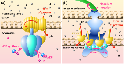
Fig.  28: : Harvesting proton gradients: energy vectorization and locomotion (a) Simplistic view of an F-type H⁺-ATPase, here working as an ATP synthesis enzyme. A proton gradient is maintained between the intermembrane space and the cytoplasm by the respiratory cycle. Protons thus naturally flow inwards through the proton channel of the ATPase (in yellow). This triggers a mechanical rotation of the central element of the ATPase that in turn catalyzes the synthesis of ATP from Adenosine diphosphate (ADP) and Phosphate (P). (b) Simplistic view of the bacterial flagellar motor (in blue). The proton gradient transverses here the stator parts of the motor (in yellow), namely the MotA/MotB complexes. These are responsible for turning the basal rotor of the flagellar motor. As the flagellum is attached to the motor, this induces rotation of the flagellum and allows for bacterial locomotion.

Proton gradients harvested for energy vectorization and locomotion – The idea that osmotic gradients could be harvested for advanced functionalities was introduced as early as in the 1960s, by the seminal work of Mitchell in Ref.358. He introduced the concept of chemi-osmotic coupling, namely that a chemical reaction may be powered by the directed channeling of a specie. In the case of the F-type ATP-ase, directed motion of protons (note that the full reaction does imply the production of water on one side of the membrane) catalyzes the synthesis of ATP through a rotary motion ³⁵⁶ – see Fig. 28-a. As the F-type catalyzes the formation of ATP (that is the vector for energy in all living systems), it is central to all forms of life ³⁵⁹. The rotary motion occurring during synthesis can be harvested for artificial locomotion of inorganic devices ³⁶⁰ . Harvesting proton gradients for locomotion is more commonly performed not by the F-type ATP-ase but by the bacterial flagellar motor ³⁶¹ – see Fig. 28-b. The bacterial flagellar motor is an impressive 45 nm ³⁶¹ ionic machinery at the root of bacterial locomotion via flagellar rotation notably in E. coli ³⁶². A proton gradient induces spontaneous transport of protons through stator parts (MotA/MotB) ³⁶³. As the transport is gated through these channels, it induces a ratchet-like motion of the rotor part of the motor ³⁶⁴. The flagellum is attached to the rotor and therefore rotates. Around 1200 ions translocating per rotation generate a force at the base of the flagellar motor of about 200 pN ³⁶¹. The flagellum rotates at about 100 Hz ³⁶¹ allowing E. coli to swim at more than 10 body lengths per second !

Nanoscale ionic machinery – The proper function of the F-type enzyme is dependent on a subtle balance of osmotic and chemical potentials for proper function ³⁶⁵ and the detailed mechanisms involving motion and electric field coupling to the proton flux are still investigated ³⁶⁶. Further physical insight on the detailed flows in the proton pump but more broadly on ionic channels is required to establish biomimetic principles to construct similar ionic machines with artificial material. Such physical insight is also dependent on better modeling of ion transport at the ultimate scales, with strong charge interactions, breakdown of hydrodynamics, etc.

6.3 Blue energy harvesting: osmotic power and capacitive mixing

As we have seen, filtration and separation of molecules requires energy input to counteract the entropy of mixing. Reversely, entropic energy harvesting may be possible by mixing molecules. The energy harvested from differences in salinity, e.g. by mixing sea water and fresh river water, is called blue energy. The maximal entropic energy collected by mixing volumes of sea and river water is typically $0.8$ kWh/m³, see Ref.367. Over the earth, counting the natural potential resources where rivers flow in the ocean such as the Amazonian river, a total of around $1$TW of power could be harvested, amounting to 8,500 TWh in a year ²⁶⁰. This is to be compared with the actual production of other renewable energies: in 2015, hydraulic energy production is $\sim$4,000 TWh, the nuclear energy around 2,600 TWh, and wind and solar 1,100 TWh altogether ³⁶⁸. In the global energy balance, blue energy, as a renewable and non-intermittent source of energy, has thus a great potential. Here we focus on some energetic and osmotic aspects of blue energy and refer to Ref.75 for a more detailed review of the current status of blue energy harvesting.

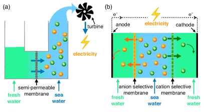
Fig.  29: : Collecting blue energy. (a) Pressure retarded osmosis (PRO). The mixing of sea water and fresh water across a semi-permeable membrane drives a water flow that turns a turbine generating energy. (b) Reverse electro-dialysis (RED). Fresh and sea water are separated by stacks of alternating cation and anion selective membranes. Spontaneous diffusion induces fluxes of ions through the selective membranes, which is captured at the boundaries by reactive electrodes producing an electric current. Usually RED is performed by alternating fresh and sea water a dozen times, although only three layers are represented on the figure.

The current attempts to harvest blue energy have essentially relied on two techniques, as sketched in Fig. 29. Pressure-retarded osmosis (PRO) harvests the natural osmotic force between sea water and river water when they are separated by a semipermeable membrane to activate a turbine to generate electricity. Reverse electro-dialysis (RED) uses diffusion gradients of salts between sea water and river water to directly generate (ionic) electric currents by separating the corresponding ion fluxes using a multi-stack of cation and anion selective membranes ³⁶⁹. Both strategies rely on separation of water from ions or ions from water, and therefore require subnanoporous structures which impede the water fluxes and diminish energetic efficiency. Current PRO technologies are only able to produce up to 3 W/m², less than the critical 5 W/m² for economic viability ³⁷⁰. The reasons for such a low performance can be readily understood: while the osmotic pressure at the interface between sea water and fresh water is considerable and reaches 30 bars, the permeability of the semi-permeable membrane is extremely small since its pore structure is in the sub-nanometer scale to sieve ions: the power, which is the product of flow rate and pressure drop is accordingly small.

On the other hand, state-of-the-art RED achieved up to 8 W/m² in controlled environment ⁸², and there is an industrial hope for blue energy harvesting which is currently explored with the REDStack project in the Netherlands ^{75, 369}.

Still we note that the above power figures should not be considered as negligible, because membrane systems are quite compact and hundreds of square meters of membranes can be packed over a single ground square meter. Such performances should be compared to the 2.5 W per square meter of ground field required for a Windmill farm ³⁷¹, due to the very large required distance between windmills to prevent flow interactions. This illustrates that blue energy is actually already competitive as such in spite of the poor performances of PRO and RED.

Beyond PRO and RED, it was shown recently that new nanomaterials and nanofluidic transport constitute key assets that allow to boost considerably these performances ^{73, 74, 75, 87, 372}. Experiments across nanotubes of boron-nitride (BN), and subsequently across MoS₂ nanoporous membranes, reported huge ionic currents.

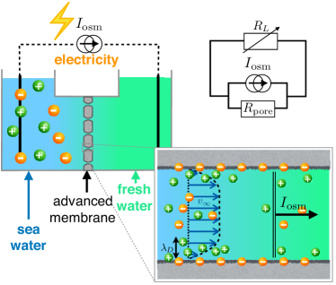
Fig.  30: : Blue energy with diffusio-osmosis. A porous membrane with large and charged pores (zoom) induces a diffusio-osmotic plug-like flow with center velocity $v_{\infty}$ upon a salt concentration difference (e.g. here between sea and fresh water) as seen in Fig. 9). This flow drives excess charges in the electric double layer producing a net ionic current $I_{\rm osm}$ that can be harvested in a load resistance $R_{L}$ – top right electric schematic.

A puzzling remark is that the BN nanotubes in the experiments of Ref.73 or the MoS₂ nanopores of Ref.74 are fully permeable to ions, in contrast to the canonical views of RED involving cation and anion selective membranes. The origin of the osmotic current was then shown to be the diffusio-osmotic ionic currents taking place at the surface of the materials, coupled to the considerable surface charge exhibited by these systems – see Fig. 30. We reported in the previous section the corresponding ionic current in Eqs.(55)-(56), and for a membrane constituted of $N$ tubes of radius $R$, length $L$ and surface charge $\Sigma$, the ionic current can be estimated as

$$I_{\rm osm}\approx N2\pi R\,\Sigma\times v_{DO}\approx N{2\pi R\over L}\Sigma\,\,D_{DO}\times\Delta\log c_{s}$$ (105)

where $v_{DO}$ the diffusio-osmotic water flow speed and $D_{DO}$ is the diffusio-osmotic mobility, typically $D_{DO}\sim k_{B}T/(8\pi\eta\ell_{B})$. This prediction was fully confirmed experimentally in Ref.73. Therefore – and this is a key asset – the blue energy does not require full selectivity of the membrane, in contrast to RED standards. Connecting the membrane to a load resistance $R_{L}$ –Fig. 30 –, the maximum osmotic power which can be harvested is easily found to be

$$\mathcal{P}=\frac{1}{4}R_{\rm pore}I_{\rm osm}^{2}$$ (106)

where $R_{\rm pore}$ is the pore or membrane resistance (that can be obtained from standard conductance measurements). Osmotic power reaches thousands of Watts per square meter in BN nanotubes, and even up to $10^{6}$W/m² for the 2D MoS₂ due to its molecular thickness (leading to huge gradients). This estimate actually suggests to couple diffusio-osmotic current generation with an asymmetric pore geometry leading to ionic diode behavior⁷⁵: blocking the ionic backflow thanks to the diode property allows one to boost the output power by reducing Joule losses (see details in Ref.75 and Fig. 30). Asymmetric channels were indeed shown to improve energy harvesting ^{373, 374}.

This methodology can be readily generalized to other materials which are better suited for upscaling as compared to BN nanotubes. Key progress has been made recently in this direction ⁷⁵. Using diffusio-osmotic currents thus constitutes a promising route for improved blue energy harvesting, making it possibly relevant to industrial scale.

Beyond these membrane-based routes, the so-called “capacitive mixing” methodology is an alternative approach to harvest osmotic energy  ³⁷⁵. The principle is to charge and discharge an ionic capacitor by alternating flows of salty and fresh water. Capacitor plates are connected to current collectors. First (step A on Fig. 31-a) salty water is flushed in, charging the capacitor plates, resulting in a closed circuit current in the load resistance. Then (step B), salty water is replaced by fresh water. When the circuit is closed again on the load resistance (step C), the capacitor plates discharge into the bulk as fresh water is less salty, resulting in a current in the opposite direction. The circuit is opened and fresh water is replaced by salty water (step D) and the cycle may start again.

The power generated may be computed from the area of the cycle in the voltage/charge plane – see Fig. 31-b. Typically, over 1 cycle (about 20h ³⁷⁶), 1 J per gram of carbon electrode may be collected. To compare with previous results, we estimate that 1 carbon plate of $6\times 6$cm² is about $1$g, such that one may recover around 0.2 W/m² with capacitive mixing. Capacitive mixing therefore requires significant progress in optimizing the cell setup and the nanoporous structure to enhance performances ^{377, 378}.

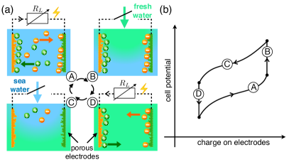
Fig.  31: : Capacitive Mixing to collect blue energy. (a) Capacitive mixing cycle. Two electrodes with functionalized surfaces (such that one is positively charged in surface (green) and the other negatively charged in surface (orange)) are embedded in a fluidic device where salty water and fresh water are alternatively flushed in a cycle. (b) Associated Voltage versus Charge cycle. The cycle is described further in the text.

6.4 Dead-end pores: Detergency, particle and liquid osmotic extraction

We have demonstrated in the previous sections how efficient diffusio-phoresis is to boost migration of particles. Combined with the ability to generate gradients of solute (in particular of salts) at small scales, it proves a method of choice in various applications to extract particles or liquids from dead-end pores. We discuss shortly two examples where diffusio-osmotic forces are harnessed.

A nice application of diffusio-osmosis was highlighted recently in the context of cleaning and the significance of rinsing in laundry detergency  ³⁷⁹. The question at stake here is how to extract particles which are stuck in dead-end pores in the porous matrix constituting the fabric. A simple flow resulting from mechanical action may not be able to perform this task, especially since particles buried in small pores in the interyarn pore space may not be recovered by advection because flow is channelled by larger pores (see Fig. 32-a and c). Experiments then showed that rinsing with fresh water generates surfactant gradients at the scale of the fabric fibres and this in turn leads to diffusio-phoretic motion of the particles inside the dead-end pores. This flushing geometry echoes the osmotic shock discussed above. As highlighted in Fig. 32-b and d, the gradient-induced motion allows one to extract particles from the intertwined network of pores. This suggests that, after laundering with any kind of detergent, rinsing with fresh water will allow a diffusio-phoretic push to wash out dirt and stains. It is worthwhile noting that detergency within this prospect also benefits from the log-sensing and osmotic shock effect discussed in Sec.5.2: particle removal by this mechanism is effective on significantly long time scales, allowing for proper removal of the particles.

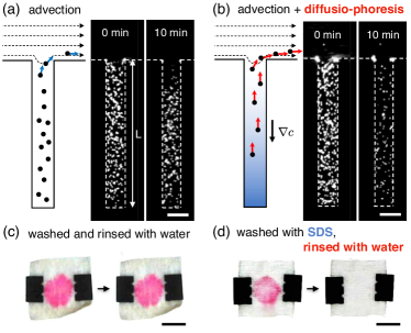
Fig.  32: : Particle removal with diffusio-phoresis. Reproduced from Ref.379 with permission from the APS, copyright 2018. (a) Fluorescence image sequence showing particles in a dead-end microfluidic pore, upon advection in the main conduct. The solutions are composed of SDS at 10 mM. (b) Same as (a) with a solute gradient, where the inner pore solute concentration is 10 mM and the outer (main channel) is 0.1 mM. All scale bars are 50 $\mu$m. (c) and (d) A piece of cotton fabric is stained with colored colloidal particles (polystyrene latex). The piece of fabric is washed and rinsed in water (c) or washed in 10 mM SDS and rinsed with water (d) then photographed immediately after rinsing (left) and 120 s afterwards (right). All scale bars are 1 cm.

This type of mechanism based on diffusio-phoretic migration is versatile and applies to any flushing geometry. Various recent experiments considered extraction of particles – colloidal particles and oil emulsions – from dead-end pores ^{209, 210}. Such results have also obvious applications in a different context, in geology for example, where dissolution and recrystallization at the mineral-fluid interface leads to ubiquituous salt gradients at the root of diffusio-phoretic and -osmotic transport ^{76, 380}. In fact, flushing by fresh water was shown to enhance considerably oil recovery, a method coined as “Low salinity enhanced oil recovery” ³⁸¹. While the very origin of this phenomenon is still debated, it is quite clear that diffusio-osmotic flows will play a key role in recovering biphasic mixtures using salinity gradients. Consider oil in a porous structure with typical pore radius $a$, as sketched in Fig. 33, where oil is trapped in dead-end pores. After a flush with fresh water, a diffusio-osmotic flow may be generated at the surface of the porous material, with velocity $v_{DO}=-D_{DO}\nabla\log c_{s}$. Assuming first that oil is blocked, this generates a counterbalancing pressure gradient, such that the total flux is vanishing, leading to a pressure drop

$$\Delta p_{DO}=-\frac{8\eta D_{DO}}{a^{2}}\Delta\left[\log c_{s}\right]$$ (107)

along the dead-end channel (and independent of the channel length). Putting in numbers, with a strong salinity gradient between salty water at 1 M and fresh water at $0.1$ mM to fix ideas, we find $\Delta p_{DO}=0.07$ bar for $a=100$nm and up to $\Delta p_{DO}=30$ bars for $a=5$nm. This has to be compared to the oil-water capillary pressure expressed as $\Delta P_{\rm cap}=\frac{\gamma}{a}$ with $\gamma\simeq 10-20$ mN$/$m a typical surface tension at the oil-water interface (possibly decorated with injected surfactants). While $\Delta p_{\rm cap}=2$ bar $>\Delta p_{DO}$ for $a=100$ nm, it is in the same range for $a=5$nm with $\Delta p_{\rm cap}\sim\Delta p_{DO}\sim 40$ bar. For very small pores, the pressure induced by diffusio-osmosis – which scales as $1/a^{2}$ – is thus able to bypass the capillary pressure, scaling as $1/a$. These simplistic estimates are made for illustration only and would deserve more detailed experimental investigations. They highlight the efficiency of diffusio-osmotic effects to extract liquids which are deeply confined within nanometric dead-end porosity.

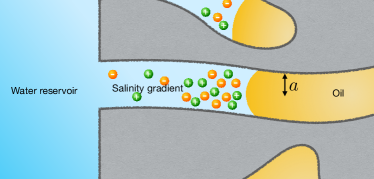
Fig.  33: : Diffusio-osmotic effects for oil recovery under salinity gradients. Enhanced oil recovery is traditionally preformed by injecting sea water in the reservoir to push the oil. However flushing with fresh water slugs is known to boost the process. Gradients of salinity within dead end pores may help bypassing the capillary forces blocking the oil within the porosity.

7 Concluding remarks and perspectives

As is clear from our discussion in the previous section, osmosis is ubiquitous and crucial to an impressive number of processes, with extremely diverse manifestations. In spite of this diversity, a key and universal aspect of osmosis is that it may be interpreted as a driving force, exerted by the membrane (or a surface, or a particle’s surface, and so on) on the solute particles. As we have seen in many situations in detail, we typically expect the apparent osmotic pressure to write generically as

$$\Delta\Pi_{\rm app}\simeq\langle c_{s}(-\nabla\mathcal{U}_{\rm eff})\rangle$$

with $\langle.\rangle$ some specific average and $\mathcal{U}_{\rm eff}$ the effective interaction potential. This mechanical perspective allows one to interpret most osmotic related phenomena (diffusio-osmosis, diffusio-phoresis, active osmosis, etc.). Beyond this generic description, a proper description of the forces at play is required in more specific examples, as we showed on the subtle example of the force balance in diffusio-phoresis.

Our understanding of osmotic related phenomena is still blurred by a number of open riddles. Non-equilibrium osmotic flows should be investigated, in particular to harvest non-equilibrium forces for advanced transport of species, which offer a number of promising avenues. Introducing more reliable descriptions and understanding for ionic transport at the smallest scales should also open the way to build advanced ionic detectors and ionic-powered machinery. At micrometric scales, a number of processes could be improved, harvesting the properties of specific geometries – as in the kidney – together with a clever mix of osmotic forces – as diffusio-phoresis for detergency.

Overall we still have a lot to learn from Nature and how it harvests osmosis in many forms, for separation purposes, energy storage and harvesting, etc. Today osmosis is usually harnessed in its most basic form, for example as the prototypical example of osmotic pressure across a semi-permeable membrane. Yet Nature has developed far more clever and far more complex examples. Mimicking the natural wonders with artificial systems is a great challenge but it opens new avenues for many outstanding societal questions that are worth the journey.

8 List of Symbols

We report below symbols that are used frequently throughout the review.

$a$	Pore radius
$\mathcal{A}$	Membrane or pore area
$b$	Slip length of the surface
$\beta$	$=1/k_{B}T$
$c_{s}$	Solute concentration
$c_{w}$	Water or solvent concentration
$c_{+/-}$	Concentration of positive or negative ions
$D_{DO}$	Diffusio-osmotic "diffusion" coefficient
$D_{DP}$	Diffusio-phoretic "diffusion" coefficient
$D_{0}$	Colloid diffusion coefficient
$D_{s}$	Diffusion coefficient of the solute
$e$	Elementary charge
$E$	Electric field
$\epsilon$	Dielectric permittivity of the fluid
$\eta$	Solvent viscosity
$I_{DO}$	Diffusio-osmotic ion current
$I_{e}$	Electric current
$J_{e}$	Exchange or Excess solute flow
$J_{s}$	Solute flow
$j_{s}$	$=J_{s}/\mathcal{A}$ Solute flow per unit area
$k_{B}$	Boltzmann’s constant
$K_{\rm osm}$	Osmotic electric mobility
$L$	Thickness of the membrane or length of the pore
$\kappa_{\rm hyd}$	Permeance of the membrane or pore
$\ell_{B}$	$=e^{2}/4\pi\epsilon k_{B}T$ Bjerrum length
$\mathbb{L}$	Transport matrix (or a part of the full matrix)
$\mathcal{L}_{D}$	$=\frac{D_{s}\mathcal{A}}{\eta L}$, Solute permeability of the membrane or pore
$\mathcal{L}_{\rm hyd}$	$=\frac{\kappa_{\rm hyd}\mathcal{A}}{\eta L}$, Hydrodynamic permeability of the membrane or pore

$\lambda$	range of potential interactions
$\lambda_{D}$	$=1/\sqrt{8\pi\ell_{B}c_{s}}$ Debye length
$\lambda_{s}$	$=\frac{D_{s}}{k_{B}T}$ mobility of the solute
$\mu_{DO}$	Diffusio-osmotic mobility
$\mu_{DP}$	Diffusio-phoretic mobility
$\mu_{EO}$	Electro-osmotic mobility
$\mu^{0}_{i}$	Chemical potential of the pure specie $i$
$\mu_{i}$	Chemical potential of specie $i$
$N_{i}$	Number of molecules of specie $i$
$\omega_{s}$	Solute "mobility" across the membrane
$p$	Pressure
$\Pi$	Osmotic pressure
$Q$	Volume flow
$R$	Particle size
$\rho_{e}$	Charge density
$\sigma$	Reflection or selectivity coefficient
$\Sigma$	Surface charge
$T$	Temperature
$\mathcal{U}(x)$	Potential barrier representing the membrane
$\bm{v}$	Velocity field of the fluid
$v_{DO}$	Diffusio-osmotic velocity
$v_{DP}$	Diffusio-phoretic velocity
$v_{EO}$	Electro-osmotic velocity
$v_{w}$	Molar volume of water
$V_{e}$	Electric potential
$X$	Solute molar fraction
$\zeta$	Zeta potential

Conflicts of interest

There are no conflicts to declare