Collaborative Similarity Embedding for Recommender Systems

Abstract.

We present collaborative similarity embedding (CSE), a unified framework that exploits comprehensive collaborative relations available in a user-item bipartite graph for representation learning and recommendation. In the proposed framework, we differentiate two types of proximity relations: direct proximity and $k$-th order neighborhood proximity. While learning from the former exploits direct user-item associations observable from the graph, learning from the latter makes use of implicit associations such as user-user similarities and item-item similarities, which can provide valuable information especially when the graph is sparse. Moreover, for improving scalability and flexibility, we propose a sampling technique that is specifically designed to capture the two types of proximity relations. Extensive experiments on eight benchmark datasets show that CSE yields significantly better performance than state-of-the-art recommendation methods.

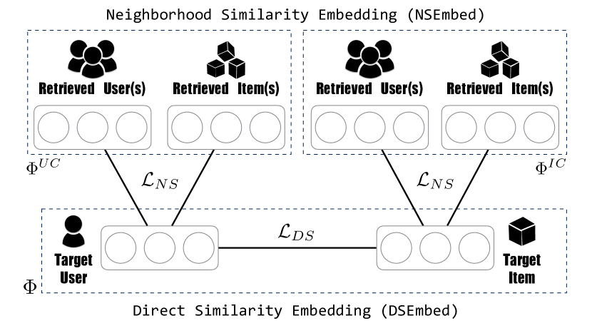
(a) The bottom part depicts the direct similarity embedding module for user-item associations, whereas the upper left (right) part corresponds to modeling user-user (item-item, respectively) similarity with the neighborhood similarity embedding module. An optimization step includes a sampled pair of a user and an item in DSEmbed and multiple high-order relation pairs in NSEmbed.

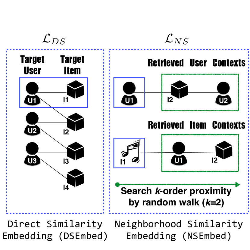
(b) The left part shows that a target user-item pair (U1-I1) can be directly sampled from the observed edges for DSEmbed; the right part shows that for U1 (or I1), a $2$-step random walk is applied to obtain the contexts used in the NSEmbed module.

Figure 1. An overview of the proposed CSE framework

1. Introduction

The task of recommender systems is to produce a list of recommendation results that match user preferences given their past behavior. Collaborative filtering (CF), a common yet powerful approach, generates user recommendations by taking advantage of the collective wisdom from all users (Jannach et al., 2016). Many CF-based recommendation algorithms have been shown to work well across various domains and been used in many real-world applications (Su and Khoshgoftaar, [n. d.]).

The core idea of model-based CF algorithms is to learn low-dimensional representations of users and items from either explicit user-item associations such as user-item ratings or implicit feedback such as playcounts and dwell time. This can be done by training a rating-based model with matrix completion to learn from observed user-item associations (either explicit or implicit feedback) to predict associations that are unobserved (Barkan and Koenigstein, 2016; Christakopoulou and Karypis, 2016; Hsieh et al., 2017; Hu et al., 2008; Koren, 2008; Koren et al., 2009; Liang et al., 2016; Ning and Karypis, 2011; Palumbo et al., 2017; Zhao et al., 2016; Salakhutdinov and Mnih, 2007). In addition to this rating-based approach, ranking-based methods have been proposed based on optimizing ranking loss; the ranking-based methods (Palumbo et al., 2017; Rendle et al., 2009; Weston et al., 2011, 2013; Yu et al., 2018) have been found more suitable for implicit feedback. However, many existing model-based CF algorithms leverage only the user-item associations available in a given user-item bipartite graph. Thus, when the available user-item associations are sparse, these algorithms may not work well.

It has been noted that it is possible to mine from a user-item bipartite graph other types of collaborative relations, such as user-user similarities and item-item similarities, since users and items can be indirectly connected in the graph. Moreover, by taking random walks on the graph, it is possible to exploit higher-order proximity among users and items. Using item-item similarities in the learning process has been firstly studied by Liang et al. (Liang et al., 2016), who propose to jointly decompose the user-item interaction matrix and the item-item co-occurrence matrix with shared item latent factors. Hsieh et al. (Hsieh et al., 2017) propose to learn a joint metric space to encode both user preferences and user-user and item-item similarities. A recent work presented by Yu et al. (Yu et al., 2018) shows that jointly modeling user-item, user-user, and item-item relations outperforms competing methods that consider only user-item relations. In (Grover and Leskovec, 2016; Perozzi et al., 2014), the higher-order proximity has been shown useful in graph embedding methods. In general, exploiting additional collaborative relations shows promise in learning better representations of vertexes in an information graph.

We note that these prior arts (Liang et al., 2016; Hsieh et al., 2017; Yu et al., 2018; Grover and Leskovec, 2016) share the same core idea: using some specific methods to sample auxiliary information from a graph to augment the data for representation learning. However, there is a lack of a unified and efficient model that generalizes the underlying computation and aims at recommendation problems. For example, Liang et al. (Liang et al., 2016) consider only the item-item similarities but no other collaborative relations; Yu et al. (Yu et al., 2018) consider only ranking-based loss functions but not rating-based ones. Higher-order proximity is exploited in (Perozzi et al., 2014; Grover and Leskovec, 2016; Gao et al., 2018), which however deal with the general graph embedding problem not the recommendation one. Moreover, the model presented by (Hsieh et al., 2017) fails to manage large-scale user-item associations (Tay et al., 2018).

To address this discrepancy, in this paper we present collaborative similarity embedding (CSE), a unified representation learning framework for collaborative recommender systems with the aim of modeling the direct and in-direct edges of user-item interactions in a simple and effective way. CSE involves a direct similarity embedding module for modeling user-item associations as well as a neighborhood similarity embedding module for modeling user-user and item-item similarities. The former module provides the flexibility to implement various types of modeling techniques for user-item associations, whereas the later module models user-user and item-item relations via $k$-order neighborhood proximity. To simultaneously manage the two modules, we introduce triplet embedding into the proposed framework to ideally model user-user, item-item clustering and user-item relations in a single and joint-learning model, while most prior arts use only one or two embedding mappings in their methods. Moreover, the two sub-modules are fused by a carefully designed sampling technique for scalability and flexibility For scalability, the space complexity and time of convergence are both only linear with respect to the number of observed user-item associations. In addition, with the proposed sampling techniques, CSE provides the flexibility to shape different relation distributions in its optimization.

Extensive experiments were conducted on eight recommendation datasets that cover different user-item interaction types, levels of data sparsity, and data sizes. We compare the performance of CSE with classic methods such as matrix factorization (MF) and Bayesian personalized ranking (BPR) (Rendle et al., 2009), recent methods that incorporate user-user and/or item-item relations (Hsieh et al., 2017; Liang et al., 2016; Yu et al., 2018), as well as several general graph embedding methods (Perozzi et al., 2014; Gao et al., 2018). The evaluation shows that CSE outperforms the competing methods for seven out of the eight datasets.

In summary, we propose a simple yet effective representation learning framework aiming at making the best use of information embedded in observed user-item associations for recommendation. Our framework advances the state-of-the-art recommendation algorithms along the following five dimensions.

1. The CSE serves as a generalized framework that models comprehensive pairwise relations among users and items with a unified objective function in a simple and effective manner.

2. The proposed sampling technique enables the suitability of CSE for large-scale user-item recommendations.

3. We provide model analyses for flexibility, scalability and time and space complexity of the proposed CSE.

4. We report extensive experiments over eight recommendation datasets covering different user-item interaction types, levels of data sparsity, and data sizes, demonstrating the robustness, efficiency, and effectiveness of our framework.

5. For reproducibility, we share the source code of CSE online at a GitHub repo, by which the learning process can be done within an hour for each dataset performed in this work.

The rest of this paper is organized as follows. In Section 2, we present the proposed CSE framework in detail, including the problem definition, the two similarity embedding modules, and the sampling techniques. We then provide model analyses for flexibility, scalability and time and space complexity of the proposed CSE in Section 3. Experimental results are provided and discussed in Section 4. Section 5 concludes the paper.

2. Proposed CSE Framework

Problem Formulation

A recommender system provides a list of ranked items to users based on their historical interactions with items. Let $U$ and $I$ denote the sets of users and items, respectively. User-item associations can be presented as a bipartite graph $G=(V,E)$, where $V=\{v_{1},\ldots,v_{|V|}\}=U\cup I$, and $E$ represents the set of observed user-item associations. Note that for explicit rating data, the weights of the user-item preference edges can be positive real numbers, whereas for implicit interactions, the bipartite graph becomes a binary graph. The goal of the CSE framework is to obtain an embedding matrix $\Phi\in\mathbb{R}^{|V|\times d}$ that maps each user and item into a $d$-dimensional embedding vector for item recommendation; that is, with the learned embedding matrix $\Phi$, for a user $v_{i}\in U$, the proposed framework generates the top-$N$ recommended items via computing the similarity between the embedding vector of the user, i.e., $\Phi_{v_{i}}$, and those of all items, i.e., $\Phi_{v_{j}}$ for all $v_{j}\in I$, where $\Phi_{v_{x}}$ denotes the row vector for vertex $v_{x}\in V$ from matrix $\Phi$.

Framework Overview

Figure 1 provides an overview of CSE. In the figure, CSE consists of two similarity embedding modules: a direct similarity embedding (DSEmbed) module to model user-item associations, and a neighborhood similarity embedding (NSEmbed) module to model user-user and item-item similarities. The DSEmbed model provides the flexibility to implement two mainstream types of modeling techniques: rating-based and ranking-based models to preserve direct proximity of user-item associations; NSEmbed, in turn, models user-user and item-item relations using the contexts within a $k$-step random walk, as shown in Fig. 1(b), to preserve $k$-order neighborhood proximity between users and items. To minimize the sum of the losses from DSEmbed and NSEmbed modules, which are denoted as $\mathcal{L}_{DS}$ and $\mathcal{L}_{NS}$ respectively, the objective function of the proposed framework is designed as

$$\mathcal{L}=\mathcal{L}_{DS}+\lambda\mathcal{L}_{NS},$$

where $\lambda$ controls the balance between the two losses. The rationale behind this design is that $\mathcal{L}_{DS}$ controls the optimization of the embedding vectors towards preserving direct user-item associations, and $\mathcal{L}_{NS}$ encourages users/items sharing similar neighbors to be close to one another in the learned embedding space.

2.1. Direct Similarity Embedding (DSEmbed) Module

Definition 2.1.

(Direct Proximity) Given a bipartite graph $G=({V,E})$, the direct proximity between a user $v_{i}\in U$ and an item $v_{j}\in I$ is represented by the presence of an edge $(v_{i},v_{j})\in E$ between these two vertices. If there is no edge between user $v_{i}$ and item $v_{j}$, then their direct proximity is defined as 0.

The DSEmbed module is designed to model the direct proximity of the user-item associations defined in Definition 2.1. For a rating-based approach, the objective is to find the embedding matrix $\Phi$ that maximizes the log-likelihood function of observed user-item pairs:

(1) $$\arg\max_{\Phi}\sum_{(v_{i},v_{j})\in E}\log p(v_{i},v_{j}|\Phi)$$

$$= \arg\min_{\Phi}\sum_{(v_{i},v_{j})\in E}-\log p(v_{i},v_{j}|\Phi).$$

In contrast, a ranking-based approach cares more about whether we can predict stronger association between a ‘positive’ user-item pair $(v_{i},v_{j})\in E$ than a ‘negative’ user-item pair $(v_{i},v_{k})\in\bar{E}$ (Rendle et al., 2009), where $\bar{E}$ denotes the set of edges for all the unobserved user-item associations. This can be approached by maximizing the log-likelihood function of observed user-item pairs over unobserved user-item pairs for each user:

(2) $$\arg\max_{\Phi}\sum_{(v_{i},v_{j},v_{k})}\log p(v_{j}>_{i}v_{k}|\Phi)$$

$$=\arg\min_{\Phi}\sum_{(v_{i},v_{j},v_{k})}-\log p(v_{j}>_{i}v_{k}|\Phi),$$

where $v_{i}\in U$ and $v_{j},v_{k}\in I$, and $>_{i}$ indicates that user $v_{i}$ prefers item $v_{j}$ over item $v_{k}$. In the above two equations, $p(v_{i},v_{j}|\Phi)$ and $p(v_{j}>_{i}v_{k}|\Phi)$ is calculated by

$$p(v_{i},v_{j}|\Phi)=\sigma\left(\Phi_{v_{i}}\cdot\Phi_{v_{j}}\right),$$

and

$$p(v_{j}>_{i}v_{k}|\Phi)=\sigma\left(\Phi_{v_{i}}\cdot\Phi_{v_{j}}-\Phi_{v_{i}}\cdot\Phi_{v_{k}}\right),$$

respectively, and $\sigma(\cdot)$ denotes the sigmoid function.

2.2. Neighborhood Similarity Embedding (NSEmbed) Module

Definition 2.2.

($k$-Order Neighborhood Proximity) Given a bipartite graph $G=({V,E})$ representing the observed user-item associations of the set of users and items in $V=U\cup I$, the $k$-order neighborhood proximity of a pair of users (or items) is defined as the similarity between their neighborhood network structures retrieved by $k$-step random walks. Mathematically speaking, given the $k$-order neighborhood structures of a pair of users (or items), $v_{i},v_{j}\in U$ (or $v_{i},v_{j}\in I$, respectively), which are denoted as two sets of neighbor nodes $N_{v_{i}}$ and $N_{v_{j}}$, with $|N_{v_{i}}|=|N_{v_{j}}|=k$, the $k$-order neighborhood proximity between $v_{i}$ and $v_{j}$ is decided by the similarity between these two sets $N_{v_{i}}$ and $N_{v_{j}}$. If there are no shared neighbors between $v_{i}$ and $v_{j}$, the neighborhood proximity between them is 0.

The NSEmbed module is designed to model $k$-order neighborhood proximity for capturing user-user and item-item similarities. Given a set of neighborhood relations for users (or items) $S_{U}=\{(v_{i},v_{j})|\ \forall v_{i}\in U,v_{j}\in N_{v_{i}}\}$ (or $S_{I}=\{(v_{i},v_{j})|\ \forall v_{i}\in I,v_{j}\in N_{v_{i}}\}$, respectively), the NSEmbed module seeks a set of embedding matrices $\Phi,\Phi^{UC},\Phi^{IC}\in\mathbb{R}^{|V|\times d}$ that maximizes the likelihood of all pairs in $S_{U}$ (or $S_{I}$, respectively), where $\Phi$ is a vertex mapping matrix akin to that used in the DSEmbed module, and $\Phi^{UC}$ and $\Phi^{IC}$ are two context mapping matrices. Note that each vertex (representing a user or an item) plays two roles for modeling the neighborhood proximity: 1) the vertex itself and 2) the context of other vertices (Perozzi et al., 2014; Tang et al., 2015; Grover and Leskovec, 2016; Zhou et al., 2017; Chen et al., 2016). With this design, the embedding vectors of vertices that share similar contexts are thus closely located in the learned vector space. Therefore, the maximization of the likelihood function can be defined as

$$\arg\max_{\Phi,\Phi^{UC},\Phi^{IC}} \prod_{(v_{i},v_{j})\in S_{U}}p(v_{j}|v_{i};\Phi;\Phi^{UC})$$

$$+\prod_{(v_{i},v_{j})\in S_{I}}p(v_{j}|v_{i};\Phi;\Phi^{IC}).$$

Similar to Eqs. (1) and (2), the above objective function becomes

(3) $$\arg\min_{\Phi,\Phi^{UC},\Phi^{IC}} \sum_{(v_{i},v_{j})\in S_{U}}-\log p(v_{j}|v_{i};\Phi;\Phi^{UC})$$

$$+\sum_{(v_{i},v_{j})\in S_{I}}-\log p(v_{j}|v_{i};\Phi;\Phi^{IC}),$$

where

(4) $$p(v_{j}|v_{i};\Theta)=\begin{cases}\sigma\left(\Phi_{v_{i}}\cdot\Phi^{UC}_{v_{j}}\right)&\quad\text{if }\,v_{i}\in U,\\ \sigma\left(\Phi_{v_{i}}\cdot\Phi^{IC}_{v_{j}}\right)&\quad\text{if }\,v_{i}\in I.\end{cases}$$

It is worth mentioning that most prior arts use only one or two embedding mappings; while the former approach fails to consider high-order neighbors (e.g., (Tang et al., 2015; Chin et al., 2016; Koren et al., 2009; Wang et al., 2015a; Guo et al., 2015)), the later one cannot model user-user, item-item, and user-item relations simultaneously (e.g., (Perozzi et al., 2014, 2016; Chen et al., 2016; Grover and Leskovec, 2016; Zhou et al., 2017; Barkan and Koenigstein, 2016)). Our newly designed triplet embedding solution (i.e., $\Theta=\{\Phi,\Phi^{UC},\Phi^{UC}\}$) can ideally model user-user, item-item clustering and user-item relations in a single and joint-learning model.

2.3. Sampling-based Expectation Loss

In order to minimize the above objective functions, we need to go through all the pairs in $E$ for Eq. (1), $E$ and $\bar{E}$ for Eq. (2), and $S_{U}$ and $S_{I}$ for Eq. (3), to compute all the pairwise losses. This is not feasible in real-world recommendation scenarios as the complexity is $\mathcal{O}(|V|\times|V|)$. To address this, we propose a sampling technique to work in tandem with the above two modules to enhance CSE’s scalability and flexibility in learning user and item representations from large-scale datasets.

In CSE, the DSEmbed and NSEmbed modules are fused with the shareable data sampling technique described below. For each parameter update, we first sample an observed user-item pair $(v_{i},v_{j})\in E$, as shown as U1 and I1 in Fig. 1(b), where $v_{i}\in U$ and $v_{j}\in I$. Then, we search for the $k$-order neighborhood structures of user $v_{i}$ and item $v_{j}$ via the $k$-step random walks. To improve computational efficiency, we use negative sampling (Tang et al., 2015). Consequently, for a rating-based approach (see Eq. (1)), the expected sampled loss of the DSEmbed module can be re-written as

(5) $$\mathcal{L}_{DS} = \mathbb{E}_{(v_{i},v_{j})\sim E}\left[\,-\log p(v_{i},v_{j}|\Phi)\,\right]+$$

$$\sum_{M}\mathbb{E}_{(v_{k},v_{h})\sim\bar{E}}\left[\,\log p(v_{k},v_{h}|\Phi)\,\right]\,,$$

where $M$ denotes the number of negative pairs adopted. For a ranking-based approach (see Eq. (2)), the DSEmbed module can be re-written as

(6) $$\mathcal{L}_{DS}=\mathbb{E}_{(v_{i},v_{k})\sim\bar{E}}\left[\mathbb{E}_{(v_{i},v_{j})\sim{E}}\left[\,-\log p(v_{j}>_{i}v_{k}|\Phi)\right]|\,v_{i}\,\right]\,.\\$$

Note that for the ranking-based approach, there is no need to explicitly include $M$ negative sample pairs as this kind of method naturally involves negative pairs from $\bar{E}$. Similarly, given a user or an item vertex $v_{i}$, its $k$-order neighborhood structure $N_{v_{i}}$ is composed of nodes in the $k$-step random walks surfing on $G$, $\mathcal{W}_{v_{i}}=(\mathcal{W}_{v_{i}}^{0},\mathcal{W}_{v_{i}}^{1},\mathcal{W}_{v_{i}}^{2},\dots,\mathcal{W}_{v_{i}}^{k})$, where the vertex for $\mathcal{W}^{j}_{v_{i}}$ is randomly chosen from the neighbors of the vertex $v$ given $\mathcal{W}_{v_{i}}^{j-1}=v$ and $\mathcal{W}_{v_{i}}^{0}=v_{i}$. The expected sampled loss of the NSEmbed module can be re-written as

(7) $$\mathcal{L}_{NS} = \mathbb{E}_{(v_{i},v_{j})\sim S_{U}}\left[\,-\log p(v_{j}|v_{i};\Phi;\Phi^{UC})\,\right]+$$

$$\sum_{M}\mathbb{E}_{(v_{i},v_{j})\sim\bar{E}}\left[\,\log p(v_{j}|v_{i};\Phi;\Phi^{UC})\,\right]+$$

$$\mathbb{E}_{(v_{i},v_{j})\sim S_{I}}\left[\,-\log p(v_{j}|v_{i};\Phi;\Phi^{IC})\,\right]+$$

$$\sum_{M}\mathbb{E}_{(v_{i},v_{j})\sim\bar{E}}\left[\,\log p(v_{j}|v_{i};\Phi;\Phi^{IC})\,\right].$$

Since $\mathcal{L}_{DS}$ and $\mathcal{L}_{NS}$ are described in a sampling-based expectation form, CSE provides the flexibility for accommodating arbitrary distributions of positive and negative data. In the following experiments, we produce the positive data according to primitive edges distribution of given user-item graph. As to negative sampling, we propose to directly sample the negative data from whole data collection instead of unobserved data collection.

2.4. Optimization

In the optimization stage, we use asynchronous stochastic gradient descent (ASGD) (Recht et al., 2011) to efficiently update the parameters in parallel. The model parameters are composed of the three embedding matrices $\Theta=\{\Phi,\Phi^{UC},\Phi^{IC}\}$, each having the size $\mathcal{O}(|V|d)$. They are updated with learning rate $\alpha$ according to

(8) $$\Theta\leftarrow\Theta-\alpha\left(\frac{\partial\mathcal{L}_{DS}}{\partial\Theta}+\lambda\left(\frac{\partial\mathcal{L}_{NS}}{\partial\Theta}\right)-\lambda_{V}\|\Phi\|\right)\,,$$

where $\lambda_{V}$ is a hyper-parameter for reducing the risk of overfitting.

[t] Dataset #Users #Items #Edges $\frac{\#\text{Edges}}{\#\text{Users}}$ Density Edge type Network type Frappe^a 957 4,028 96,202 100.52 2.50% click count app-clicks CiteULike^b 5,551 16,980 210,504 37.92 0.22% like/dislike references Netflix^c 65,533 17,759 25,120,129 383.32 2.15% 5-star movie-ratings MovieLens-Latest^d 259,137 40,110 24,404,096 94.17 0.23% 5-star movie-ratings Last.fm-360K^e 359,347 294,015 17,559,530 48.86 0.02% play count artist-plays Amazon-Book^f 603,668 367,982 8,898,041 14.73 0.004% 5-star book-ratings Epinions-Extend^g 755,760 120,492 13,668,319 18.08 0.02% 5-star product-reviews Echonest^h 1,019,318 384,546 48,373,586 47.45 0.01% play count song-plays

Table 1. Statistics of the datasets considered in our experiments.

• http://baltrunas.info/research-menu/frappe

• http://www.wanghao.in/CDL.htm

• http://academictorrents.com/

• https://grouplens.org/

• http://www.dtic.upf.edu//~ocelma/MusicRecommendationDataset/

• http://jmcauley.ucsd.edu/data/amazon/

• http://www.trustlet.org/epinions.html

• https://labrosa.ee.columbia.edu/millionsong/tasteprofile

3. Model Analysis

The CSE framework not only modularizes the modeling of pairwise user-item, user-user, and item-item relations, but also integrates them into a single objective function through shared embedding vectors. Together with the DSEmbed and NSEmbed sub-modules for modeling these relations, CSE involves a novel sampling technique to improve scalability and flexibility. To give a clear view of CSE, we further provide the comparison to general graph embedding and deep learning models.

3.1. Scalability

Typical factorization methods usually work on a sparse user-item matrix and do not explicitly model high-order connections from the corresponding user-item bipartite graph $G=(V,E)$. Several methods, including our CSE, propose to explicitly incorporate high-order connections for modeling user-user and item-item relations into the recommendation models to improve performance. As discussed in (Levy and Goldberg, 2014; Liang et al., 2016; Mikolov et al., 2013), such modeling can then be seen as conducting matrix factorization on a $|V|\times|V|$ point-wise mutual information (PMI) matrix:

$$\text{PMI}\,(v_{i},v_{j})=\log\left(\frac{p(v_{i},v_{j})}{p(v_{i})p(v_{j})}\right)-\log M\,.$$

Recall that $V=U\cup I$, and $M$ denotes the number of negative pairs adopted in Eqs. (5) and (7). However, given the high-order connections for modeling user-user and item-item relations, most $\text{PMI}(v_{i},v_{j})$ for $v_{i},v_{j}\in U$ (or $v_{i},v_{j}\in I$) are nonzero and thus the PMI matrix is considered non-sparse. Conducting matrix factorization on such a matrix is computationally expensive in both time and space, and is therefore infeasible in many large-scale recommendation scenarios.

To explicitly consider all the collaborative relations into our model while keeping it practical for large-scale datasets, the CSE uses the sampling technique together with $k$-step random walks surfing on $G$ to preserve direct proximity of user-item associations as well as harvest the high-order neighborhood structures of users and items. By doing so, we approximate factorization of the corresponding PMI matrix and thus reduce the complexity in space and the training time.

3.2. Flexibility

In the CSE, the DSEmbed and NSEmbed modules are united with the sampling technique. In addition to improved scalability, such a sampling perspective facilitates the shaping of different relation distributions for optimization via different weighting schemes or sampling strategies. Here we resort to use the perspective of KL divergence to explain this model characteristic. Specifically, minimizing the losses in our framework (see Eqs. (5), (6), and (7)) can be related to minimizing the KL divergence of two probability distributions (Tang et al., 2015). Suppose there are two distributions over the space $V\times V$: $\hat{p}(\cdot,\cdot)$ and $p(\cdot,\cdot)$, denoting the empirical distribution and the target distribution, respectively, we have

(9) $$\arg\min_{p}\text{KL}(\hat{p}(\cdot,\cdot),p(\cdot,\cdot))$$

$$= \arg\min_{p}-\sum_{(v_{i},v_{j})\in E}\hat{p}(v_{i},v_{j})\log\left(\frac{p(v_{i},v_{j})}{\hat{p}(v_{i},v_{j})}\right)$$

$$\propto \arg\min_{p}-\sum_{(v_{i},v_{j})\in E}\hat{p}(v_{i},v_{j})\log p(v_{i},v_{j}).$$

In Eq. (9), the empirical distribution $\hat{p}(\cdot,\cdot)$ can be treated as the probability density (mass) function of the distribution in our loss functions, from which each pair of vertices $(v_{i},v_{j})$ is sampled. This indicates that applying different weighting schemes or different sampling strategies (i.e., different $\hat{p}(\cdot,\cdot)$) in CSE shapes different relation distributions for learning representations.

3.3. Complexity

The time and space complexity of the proposed method depends on the implementation. The training procedure of CSE framework involves a sampling step and an optimization step. Since all the required training pairs, including observed associations and unobserved associations, can be derived from the user-item bipartite graph $G$, we adopt the compressed sparse alias rows (CSAR) data structure to perform weighted edge sampling for direct similarity and weighted random walk for neighborhood similarity (Chen et al., 2017). With CSAR data structure, sampling an edge requires only $\mathcal{O}(1)$ and the overall demand space complexity is linearly increased with the number of positive edges $\mathcal{O}(|E|)$. As to the optimization, SGD-based update has a closed form so that updating the embedding of a vertex in a batch depends only on the dimension size $O(d)$. As for the time of convergence, many studies on graph embedding as well as our method empirically show that the required total training time for the convergence of embedding learning is also linear in $|E|$ (Gu et al., 2018).

3.4. Comparison to General Graph Embedding Models

General graph embedding algorithms, such as DeepWalk (Perozzi et al., 2014) and node2vec (Grover and Leskovec, 2016), can be used for the task of recommendation. Yet, we do not focus on comparing the proposed CSE with general graph embedding models and only provide the results of DeepWalk because many prior works on recommendation (Palumbo et al., 2017; Zhao et al., 2016) have shown that many of the baseline methods considered in our paper outperform these general graph embedding algorithms. The main reason for this phenomenon is that most graph embedding methods cluster vertices that have similar neighbors together, and thus make the users apart from the items because user-item interactions typically form a bipartite graph.

3.5. Comparison to Deep Learning Models

Our method, and the existing methods we discussed and compared in the experiments, focus on improving the modeling quality of user and item embeddings that can be directly and later used for user-item recommendation with similarity computation. Many approximation techniques, such as approximate nearest neighbor(ANN), can be applied to speed up the similarity computation between user and item embeddings, which facilitates real-time online predictions and makes the recommendation scalable to large-scale real-world datasets. In contrast, many deep learning methods, including NCF (He et al., 2017), DeepFM (Guo et al., 2017), etc, do not learn the directly comparable embeddings of users or items. There are a few deep learning methods (e.g., Collaborative Deep Embedding (Wang et al., 2015b) and DropoutNet (Volkovs et al., 2017)) that can produce user and item embeddings, but to our knowledge, efficiency is still a major concern of these methods. Therefore, improving the embedding quality is still a critical research issue for building up a recommender system especially when the computation power is limited in real-world application scenarios. For readability and to maintain the focus of this work, we opt for not comparing the deep learning methods in our paper. It is also worth mentioning that our solution can obtain user and item embeddings within only an hour for every large dataset listed in the paper; the efficiency and scalability is thus one of the highlights of the proposed method.

4. Experiment

4.1. Settings

4.1.1. Datasets and Preprocessing

To examine the capability and scalability of the proposed CSE framework, we conducted experiments on eight publicly available real-world datasets that vary in terms of domain, size, and density, as shown in Table 1. For each of the datasets, we discarded the users who have less than ten associated interactions with items. In addition, we converted each data into implicit feedback: 1) for 5-star rating datasets, we transformed ratings higher than or equal to 3.5 to 1 and the rest to 0; 2) for count-based datasets, we transformed counts higher than or equal to 3 to 1 and the rest to 0; 3) for the CiteULike dataset, no transformation was conducted as it is already a binary preference dataset.

4.1.2. Baseline Algorithms

We compare the performance of our model with the following eight baseline methods: 1) POP, a naive popularity model that ranks the items by their degrees, 2) DeepWalk (Perozzi et al., 2014), a classic algorithm of network embedding, 3) WALS (Hu et al., 2008), a weighted rating-based factorization model, 4) ranking-based factorization models: BPR (Rendle et al., 2009), WARP (Weston et al., 2011), and $K$-OS (Weston et al., 2013), 5) BiNE (Gao et al., 2018), a network embedding model specialized for bipartite networks, and 6) recent advanced models considering user-user/item-item relations: coFactor (Liang et al., 2016), CML (Hsieh et al., 2017) and WalkRanker (Yu et al., 2018), Note that except for POP, the embedding vectors for users and items learned by these competitors as well as by our method can be directly used for item recommendations. Additionally, while CML adopts Euclidean distance as the scoring function, all other methods including ours utilize the dot product to calculate the score of a pair of user-item embedding vectors. The experiments for WALS and BPR were conducted using the matrix factorization library QMF, and those for WARP and $K$-OS were conducted using LightFM; for coFactor, CML, and WalkRanker, we used the code provided by the respective authors.

4.1.3. Experimental Setup

For all the experiments, the dimension of embedding vectors was fixed to 100; the values of the hyper-parameters for the compared method were decided via implementing a grid search over different settings, and the combination that leads to the best performance was picked. The ranges of hyper-parameters we searched for the compared methods are listed as follows.

• learning rate: [0.0025, 0.01, 0.025, 0.1]

• regularization: [0.00025, 0.001, 0.0025, 0.01, 0.025, 0.1]

• training epoch: [10, 20, 40, 80, 160]

• sampling time: [$20\times|E|$, $40\times|E|$, $60\times|E|$, $80\times|E|$, $100\times|E|$]

• walk time: [10, 40, 80]

• walk length: [40, 60, 80]

• window size: [2, 3, 4, 5, 6, 8, 10]

• stopping probability for random walk: [0.15, 0.25, 0.5, 0.75]

• $k$-order: [1, 2, 3]

• rank margin: 1 (commonly used default value)

• number of negative samples: 5 (commonly used default value)

For our model, the learning rate $\alpha$ was set to 0.1, $\lambda_{V}$ was set to 0.025; the hyper-parameter $\lambda$ was set to 0.05 and 0.1 for rating-based CSE and ranking-based CSE, respectively, and $k$ was set to 2 as the default value. The sensitivity of CSE parameters are additionally reported. For each dataset, the sample time for convergence depends on the number of non-zero user-item interaction edges and is set to $80\times|E|$. Sensitivity analysis for $k$ and $\lambda$ and convergence analysis are later provided in the section for convergence analyses.

	Frappe		CiteULike		Netflix		MovieLens-Latest
	Recall@10	mAP@10	Recall@10	mAP@10	Recall@10	mAP@10	Recall@10	mAP@10
Pop	0.1750	0.0708	0.0270	0.0114	0.0861	0.0359	0.0882	0.0289
DeepWalk (Perozzi et al., 2014)	0.0430	0.0256	0.0875	0.0458	0.0235	0.0112	0.0207	0.0061
WALS (Hu et al., 2008)	0.1632	0.1117	0.1851	0.0915	0.1214	0.0471	0.2350	$\dagger$0.1682
BPR (Rendle et al., 2009)	0.2785	0.1550	0.0861	0.0426	0.1496	0.0757	0.2163	0.1130
WARP (Weston et al., 2011)	0.3012	0.1796	0.1468	0.0813	$\dagger$0.1887	$\dagger$0.1004	$\dagger$0.2712	0.1651
$K$-OS (Weston et al., 2013)	0.3018	0.1914	0.1356	0.0756	0.1783	0.0868	0.2522	0.1641
BiNE (Gao et al., 2018)	0.2159	0.1201	0.0422	0.0201	-	-	-	-
coFactor (Liang et al., 2016)	0.2110	0.1309	0.1323	0.0721	-	-	-	-
CML (Hsieh et al., 2017)	$\dagger$0.3311	0.1958	0.1740	0.1008	0.1035	0.0444	0.1109	0.0957
WalkRanker (Yu et al., 2018)	0.3286	$\dagger$0.2099	$\dagger$0.2059	$\dagger$0.1192	0.1090	0.0483	0.1307	0.0351
RATE-CSE	0.3347	0.2047	*0.2362	*0.1452	*0.2014	*0.1039	*0.3225	*0.1990
Improv. (%)	$+$1.0%	$-$2.4%	$+$14.7%	$+$21.9%	$+$6.7%	$+$3.5%	$+$18.9%	$+$18.3%
RANK-CSE	0.3155	0.2005	0.1993	*0.1228	*0.2156	*0.1202	*0.3094	*0.1902
Improv. (%)	$-$4.7%	$-$4.4%	$-$3.2%	$+$3.0%	$+$14.2%	$+$19.7%	$+$14.1%	$+$13.1%

	Last.fm-360K		Amazon-Book		Epinions-Extend		Echonest
	Recall@10	mAP@10	Recall@10	mAP@10	Recall@10	mAP@10	Recall@10	mAP@10
Pop	0.0309	0.0133	0.0053	0.0015	0.0450	0.0246	0.0257	0.0104
WALS (Hu et al., 2008)	0.1621	0.0857	$\dagger$0.0540	$\dagger$0.0227	0.1479	0.0634	0.1287	$\dagger$0.0638
BPR (Rendle et al., 2009)	0.1120	0.0545	0.0248	0.0119	0.1126	0.0579	0.0499	0.0210
WARP (Weston et al., 2011)	0.1556	0.0832	0.0457	0.0199	$\dagger$0.1509	$\dagger$0.0775	0.1001	0.0447
$K$-OS (Weston et al., 2013)	$\dagger$0.1641	$\dagger$0.0888	0.0511	0.0215	0.1493	0.0766	$\dagger$0.1249	0.0597
CML (Hsieh et al., 2017)	0.0496	0.0199	0.0129	0.0052	0.1171	0.0629	0.0357	0.0195
WalkRanker (Yu et al., 2018)	0.0233	0.0088	0.0080	0.0036	0.0560	0.0289	0.0309	0.0133
RATE-CSE	*0.1687	*0.0909	0.0540	0.0240	*0.1659	0.0788	0.1260	0.0605
Improv. (%)	$+$2.8%	$+$2.3%	$+$0.0%	$+$5.7%	$+$9.9%	$+$1.7%	$+$0.8%	$-$0.5%
RANK-CSE	*0.1762	*0.0970	*0.0625	*0.0274	*0.1767	*0.0921	*0.1358	*0.0679
Improv. (%)	$+$8.2%	$+$14.4%	$+$15.7%	$+$20.7%	$+$17.0%	$+$20.2%	$+$8.7%	$+$6.4%

Table 2. Recommendation performance. The $\dagger$ symbol indicates the best performing method among all the baseline methods; ‘*’ and ‘%Improv.’ denote statistical significance at $p<0.01$ with a paired $t$-test and the percentage improvement of the proposed method, respectively, with respect to the best performing baseline.

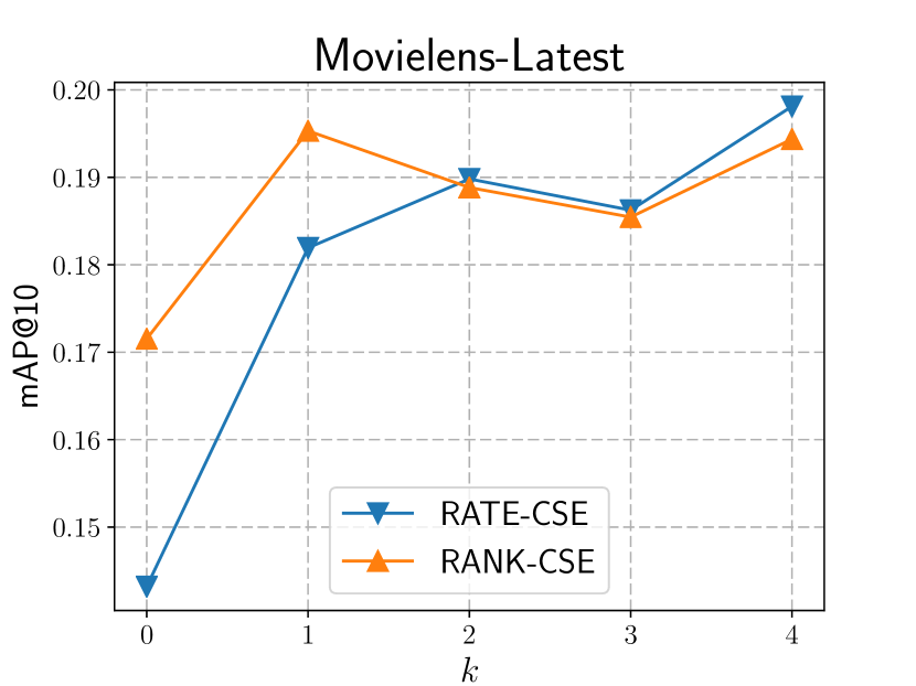
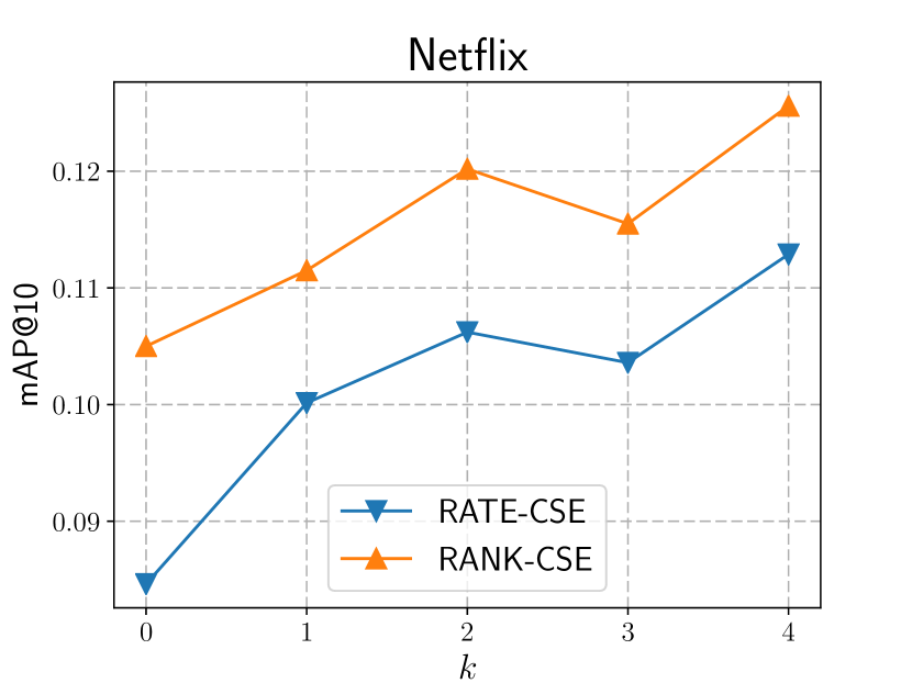
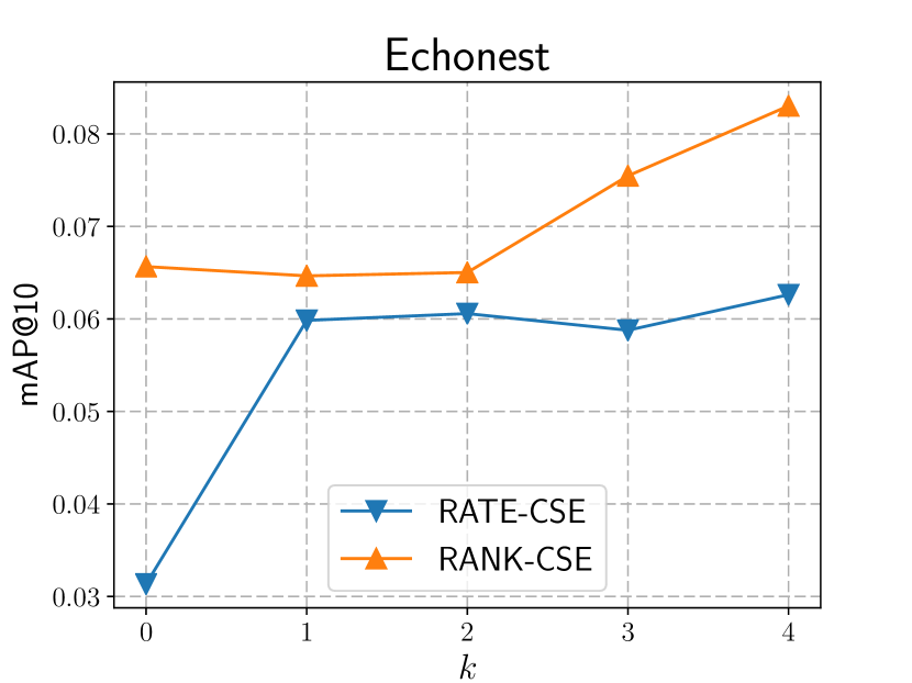
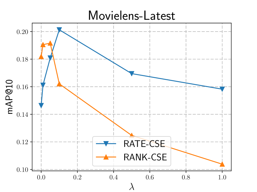
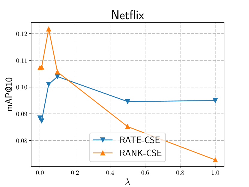
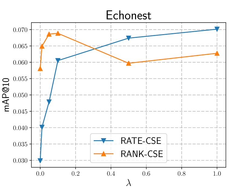
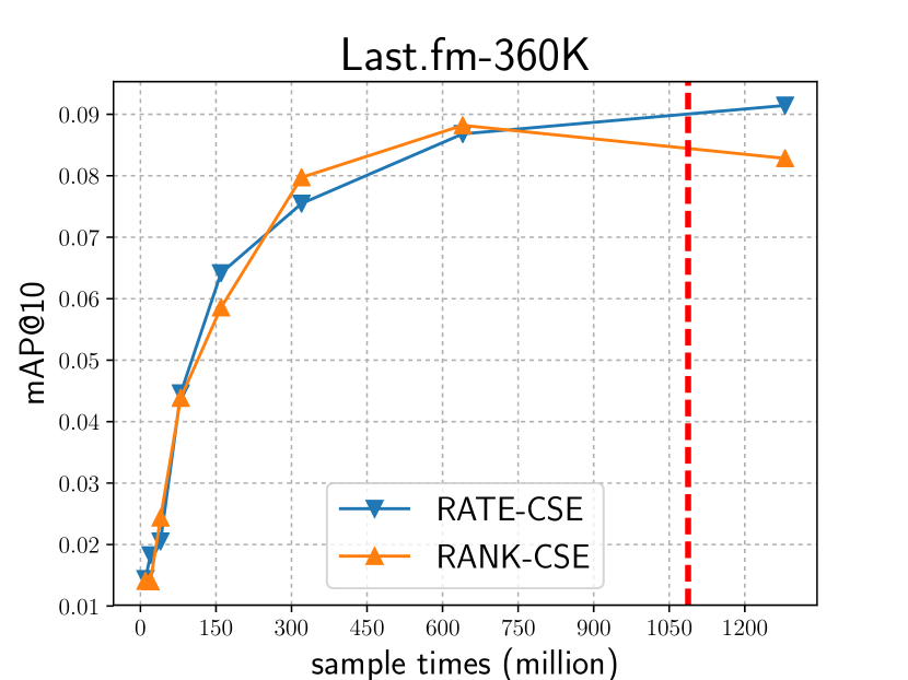
Figure 2. Sensitivity and convergence analyses

4.1.4. Evaluations

The performance is evaluated between the recommended list $R_{u}$ containing top-$N$ recommended items and the corresponding ground truth list $T_{u}$ for each user $u$. We consider following two commonly-used metrics over these $N$ recommended results:

• Recall: Denoted as Recall@$N$, which describes the fraction of the ground truth (i.e., the user preferred items) that are successfully recommended by the recommendation algorithm:

  $$\text{Recall@}N=\sum_{u\in U}\frac{1}{|U|}\frac{\sum_{v\in R_{u}}\mathbbm{1}(v\in T_{u})}{\min(N,|T_{u}|)}.$$

• Mean Average Precision: Denoted as mAP@$N$, computing the mean of the average precision at $k$ (AP@$k$) for each user $u$ as

  $$\text{mAP@}N = \frac{1}{|U|}\sum_{u\in U}\text{AP}_{u}@k$$

  $$= \frac{1}{|U|}\sum_{u\in U}\frac{\sum_{k=1}^{N}\text{P}_{u}(k)\times\mathbbm{1}(r_{k}\in T_{u})}{\min(N,|T_{u}|)},$$

where $r_{k}$ is the $k$-th recommended item and $\text{P}_{u}(k)$ denotes the precision at $k$ for user $u$. This is a rank-aware evaluation metric because it considers the positions of each recommended item. For each dataset, the reported performance was averaged over 10 times; in each time, we randomly split the data into 80% training set and 20% testing set.

4.2. Results

4.2.1. Recommendation Performance Comparison

The results for the ten baseline methods along with the proposed method are listed in Table 2, where RATE-CSE and RANK-CSE denote two versions of our method that employ respectively rating-based and ranking-based loss functions for user-item associations. Note that the best results are always indicated by the bold font, and for coFactor and BiNE we report only the experimental results on Frappe and CiteULike because of resource limitations. As discussed in Section 3.4, DeepWalk is not suitable for user-item recommendation as it make the users apart from items in the embedding space. In addition, observe that BiNE does not perform well in our experiments; such a result is due to the fact that BiNE is a general network embedding model and thus does not incorporate the regularizer in their objective function, which is however an important factor for the robustness of recommendation performance. Comparing the performance of the other baseline methods, we observe that the performance of WALS, WARP and $K$-OS is very competitive. That is, these methods achieve the top performance among all the baselines on several datasets. The performance of WalkRanker and CML, on the other hand, seems satisfactory only on two rather small datasets – Frappe and CiteULike – and performs more poorly on most of the other datasets.

We observe that our method achieves the best results in terms of both Recall@10 and mAP@10 for most datasets. Moreover, RANK-CSE generally outperforms RATE-CSE in the experiments, re-confirming that using a ranking-based loss is indeed better for datasets with binary implicit feedbacks (Rendle et al., 2009; Weston et al., 2011, 2013). Specifically, except for Frappe, RATE-CSE or RANK-CSE achieves significantly much better performance than the best performing baseline methods with a maximum improvement of +20.7%.

4.2.2. Parameter Sensitivity and Convergence Analyses

Figure 2 shows the results of the sensitivity analysis on two hyper-parameters $k$ and $\lambda$ in the first and second rows, respectively, and those of the convergence analysis based on sample times in the third row. We first observe that increasing the order $k$ of modeling neighborhood proximity between users or items improves the performance in general. We first observe from Figure 2 is that the optimal value of $k$ is data dependent and has to be empirically tuned considering the trade-off between accuracy and time/space complexity. In general, a larger $k$ leads to better result, and from our experience, the result would reach a plateau when $k$ is sufficiently large (e.g., when $k>3$). The second row of Figure 2 shows how the balancing parameter $\lambda$ affects performance: RANK-CSE obtains better performance with a value around 0.05, while RATE-CSE performs well with a value around 0.1. Finally, we empirically show that the required total sample times for convergence is linear with respect to $|E|$ as illustrated in the third row, where the vertical dash line indicates the boundary of $|E|\times 80$ as we applied to the previous recommendation experiment. As the training time depends linearly on the sample times, it can be said that both RATE-CSE and RANK-CSE converge with less than a constant multiple of $|E|$ sample times. This demonstrates the nice scalability of CSE.

5. Conclusion

We present CSE, a unified representation learning framework that exploits comprehensive collaborative relations available in a user-item bipartite graph for recommender systems. Two types of proximity relations are modeled by the proposed DSEmbed and NSEmbed modules. Moreover, we propose a sampling technique to enhance the scalability and flexibility of the model. Experimental results show that CSE yields superior recommendation performance over a wide range of datasets with different sizes, densities, and types than many state-of-the-art recommendation methods.

References

- (1)
- Barkan and Koenigstein (2016) Oren Barkan and Noam Koenigstein. 2016. Item2Vec: Neural item embedding for collaborative filtering. In Workshop IEEE MLSP.
- Chen et al. (2017) Chih-Ming Chen, Yi-Hsuan Yang, Yian Chen, and Ming-Feng Tsai. 2017. Vertex-Context Sampling for Weighted Network Embedding. CoRR (2017).
- Chen et al. (2016) Chih-Ming Chen, Ming-Feng Tsai, Yu-Ching Lin, and Yi-Hsuan Yang. 2016. Query-based Music Recommendations via Preference Embedding. In Proc. ACM RecSys.
- Chin et al. (2016) Wei-Sheng Chin, Bo-Wen Yuan, Meng-Yuan Yang, Yong Zhuang, Yu-Chin Juan, and Chih-Jen Lin. 2016. LIBMF: A Library for Parallel Matrix Factorization in Shared-memory Systems. Journal of Machine Learning Research (2016).
- Christakopoulou and Karypis (2016) Evangelia Christakopoulou and George Karypis. 2016. Local Item-Item Models For Top-N Recommendation. In Proc. ACM RecSys.
- Gao et al. (2018) Ming Gao, Leihui Chen, Xiangnan He, and Aoying Zhou. 2018. BiNE: Bipartite Network Embedding. In Proc. ACM SIGIR.
- Grover and Leskovec (2016) Aditya Grover and Jure Leskovec. 2016. Node2Vec: Scalable Feature Learning for Networks. In Proc. ACM SIGKDD.
- Gu et al. (2018) Yupeng Gu, Yizhou Sun, Yanen Li, and Yang Yang. 2018. RaRE: Social Rank Regulated Large-scale Network Embedding. In Proc. WWW.
- Guo et al. (2015) Guibing Guo, Jie Zhang, and Neil Yorke-Smith. 2015. TrustSVD: Collaborative Filtering with Both the Explicit and Implicit Influence of User Trust and of Item Ratings. In Proc. AAAI.
- Guo et al. (2017) Huifeng Guo, Ruiming Tang, Yunming Ye, Zhenguo Li, and Xiuqiang He. 2017. DeepFM: A Factorization-Machine based Neural Network for CTR Prediction. CoRR (2017).
- He et al. (2017) Xiangnan He, Lizi Liao, Hanwang Zhang, Liqiang Nie, Xia Hu, and Tat-Seng Chua. 2017. Neural Collaborative Filtering. In Proc. WWW.
- Hsieh et al. (2017) Cheng-Kang Hsieh, Longqi Yang, Yin Cui, Tsung-Yi Lin, Serge Belongie, and Deborah Estrin. 2017. Collaborative Metric Learning. In Proc. WWW.
- Hu et al. (2008) Yifan Hu, Yehuda Koren, and Chris Volinsky. 2008. Collaborative Filtering for Implicit Feedback Datasets. In Proc. IEEE ICDM.
- Jannach et al. (2016) Dietmar Jannach, Paul Resnick, Alexander Tuzhilin, and Markus Zanker. 2016. Recommender systems—beyond matrix completion. Commun. ACM (2016).
- Koren (2008) Yehuda Koren. 2008. Factorization Meets the Neighborhood: A Multifaceted Collaborative Filtering Model. In Proc. ACM KDD.
- Koren et al. (2009) Yehuda Koren, Robert Bell, and Chris Volinsky. 2009. Matrix Factorization Techniques for Recommender Systems. (2009).
- Levy and Goldberg (2014) Omer Levy and Yoav Goldberg. 2014. Neural Word Embedding As Implicit Matrix Factorization. In Proc. NIPS.
- Liang et al. (2016) Dawen Liang, Jaan Altosaar, Laurent Charlin, and David M. Blei. 2016. Factorization Meets the Item Embedding: Regularizing Matrix Factorization with Item Co-occurrence. In Proc. ACM RecSys.
- Mikolov et al. (2013) Tomas Mikolov, Ilya Sutskever, Kai Chen, Greg Corrado, and Jeffrey Dean. 2013. Distributed Representations of Words and Phrases and Their Compositionality. In Proc. NIPS.
- Ning and Karypis (2011) Xia Ning and George Karypis. 2011. SLIM: Sparse Linear Methods for Top-N Recommender Systems. In Proc. IEEE ICDM.
- Palumbo et al. (2017) Enrico Palumbo, Giuseppe Rizzo, and Raphaël Troncy. 2017. entity2rec: Learning User-Item Relatedness from Knowledge Graphs for Top-N Item Recommendation. In Proc. ACM RecSys.
- Perozzi et al. (2014) Bryan Perozzi, Rami Al-Rfou, and Steven Skiena. 2014. DeepWalk: Online Learning of Social Representations. In Proc. ACM SIGKDD.
- Perozzi et al. (2016) Bryan Perozzi, Vivek Kulkarni, and Steven Skiena. 2016. Walklets: Multiscale Graph Embeddings for Interpretable Network Classification. CoRR (2016).
- Recht et al. (2011) Benjamin Recht, Christopher Re, Stephen Wright, and Feng Niu. 2011. HOGWILD!: A Lock-Free Approach to Parallelizing Stochastic Gradient Descent. In Proc. NIPS.
- Rendle et al. (2009) Steffen Rendle, Christoph Freudenthaler, Zeno Gantner, and Lars Schmidt-Thieme. 2009. BPR: Bayesian Personalized Ranking from Implicit Feedback]. In Proc. UAI.
- Salakhutdinov and Mnih (2007) Ruslan Salakhutdinov and Andriy Mnih. 2007. Probabilistic Matrix Factorization. In Proc. NIPS.
- Su and Khoshgoftaar ([n. d.]) Xiaoyuan Su and Taghi M Khoshgoftaar. [n. d.]. A survey of collaborative filtering techniques. Advances in artificial intelligence 2009 ([n. d.]).
- Tang et al. (2015) Jian Tang, Meng Qu, Mingzhe Wang, Ming Zhang, Jun Yan, and Qiaozhu Mei. 2015. LINE: Large-scale Information Network Embedding. In Proc. WWW.
- Tay et al. (2018) Yi Tay, Luu Anh Tuan, and Siu Cheung Hui. 2018. Latent Relational Metric Learning via Memory-based Attention for Collaborative Ranking. In Proc. WWW.
- Volkovs et al. (2017) Maksims Volkovs, Guangwei Yu, and Tomi Poutanen. 2017. DropoutNet: Addressing Cold Start in Recommender Systems. In Proc. NIPS.
- Wang et al. (2015a) Hao Wang, Naiyan Wang, and Dit-Yan Yeung. 2015a. Collaborative Deep Learning for Recommender Systems. In Proc. ACM KDD.
- Wang et al. (2015b) Hao Wang, Naiyan Wang, and Dit-Yan Yeung. 2015b. Collaborative Deep Learning for Recommender Systems. In Proc. ACM SIGKDD.
- Weston et al. (2011) Jason Weston, Samy Bengio, and Nicolas Usunier. 2011. WSABIE: Scaling Up to Large Vocabulary Image Annotation. In Proc. IJCAI.
- Weston et al. (2013) Jason Weston, Hector Yee, and Ron J. Weiss. 2013. Learning to Rank Recommendations with the K-order Statistic Loss. In Proc. ACM RecSys.
- Yu et al. (2018) Lu Yu, Chuxu Zhang, Shichao Pei, Guolei Sun, and Xiangliang Zhang. 2018. WalkRanker: A Unified Pairwise Ranking Model with Multiple Relations for Item. In Proc. AAAI.
- Zhao et al. (2016) Wayne Xin Zhao, Jin Huang, and Ji-Rong Wen. 2016. Learning Distributed Representations for Recommender Systems with a Network Embedding Approach.. In AIRS.
- Zhou et al. (2017) Chang Zhou, Yuqiong Liu, Xiaofei Liu, Zhongyi Liu, and Jun Gao. 2017. Scalable Graph Embedding for Asymmetric Proximity. In Proc. AAAI.