Non-crossing run-and-tumble particles on a line

Abstract

We study active particles performing independent run and tumble motion on an infinite line with velocities $v_{0}\sigma(t)$, where $\sigma(t)=\pm 1$ is a dichotomous telegraphic noise with constant flipping rate $\gamma$. We first consider one particle in the presence of an absorbing wall at $x=0$ and calculate the probability that it has survived up to time $t$ and is at position $x$ at time $t$. We then consider two particles with independent telegraphic noises and compute exactly the probability that they do not cross up to time $t$. Contrarily to the case of passive (Brownian) particles this two-RTP problem can not be reduced to a single RTP with an absorbing wall. Nevertheless, we are able to compute exactly the probability of no-crossing of two independent RTP’s up to time $t$ and find that it decays at large time as $t^{-1/2}$ with an amplitude that depends on the initial condition. The latter allows to define an effective length scale, analogous to the so called “ Milne extrapolation length” in neutron scattering, which we demonstrate to be a fingerprint of the active dynamics.

I Introduction

First-passage properties of a single or multiple Brownian walkers have been studied extensively with a tremendous range of applications in physics, chemistry, biology, astronomy, and all the way to computer science and finance (for reviews see e.g., Refs. Chandra_1943 ; Redner_book ; SM_review ; BF_2005 ; Persistence_review ; fp_book_2014 amongst many others). As a warmup, let us start, for example, with the simple problem of computing the probability that two ordinary Brownian particles on an infinite line, initially separated by a positive distance, do not cross each other up to time $t$. Starting initially at $x(0)$ and $y(0)$, with $x(0)>y(0)$, the positions $x(t)$ and $y(t)$ of the two walkers evolve independently by the Langevin dynamics

$$\frac{dx}{dt}=\eta_{1}(t)\,;\quad\frac{dy}{dt}=\eta_{2}(t)\,,$$ (1)

where $\eta_{1}(t)$ and $\eta_{2}(t)$ are independent Gaussian white noises with zero mean and correlators $\langle\eta_{i}(t)\eta_{j}(t^{\prime})\rangle=2D\,\delta_{i,j}\,\delta(t-t^{\prime})$ for $i,\,j=1,\,2$. What is the probability that two particles do not cross each other up to time $t$?

This classic first-passage question can be solved very easily by considering the relative coordinate $z(t)=[x(t)-y(t)]/2$ that also evolves as a Brownian motion

$$\frac{dz}{dt}=\eta(t)\,$$ (2)

where $\eta(t)=[\eta_{1}(t)-\eta_{2}(t)]/2$ is again a Gaussian white noise with zero mean and correlator $\langle\eta(t)\eta(t^{\prime})\rangle=2\,D^{\prime}\,\delta(t-t^{\prime})$ with an effective diffusion constant $D^{\prime}=D/2$. The initial value of $z(t)$ is simply $z_{0}=[x(0)-y(0)]/2>0$. Thus, the non-crossing probability of two particles reduces to the no zero crossing probability of a single particle: what is the probability that a single Brownian walker, starting initially at $z_{0}>0$, does not cross the origin up to time $t$? This resulting single particle problem can be solved quite easily by the image method Chandra_1943 ; Redner_book ; Persistence_review ; SM_review . Let $P(z,t|z_{0})$ denote the probability density that the walker is at $z$ at time $t$ starting from $z_{0}$ at $t=0$ and that it has not yet crossed the origin during the time interval $[0,t]$. Then, $P(z,t|z_{0})$ satisfies the diffusion equation, $\partial_{t}P=D^{\prime}\,\partial_{z}^{2}P$, on the semi-infinite line $z\geq 0$ with an absorbing boundary condition at the wall $z=0$ (origin) and the initial condition $P(z,t=0|z_{0})=\delta(z-z_{0})$. The exact solution, obtained simply via the image method, reads

$$P(z,t|z_{0})=\frac{1}{\sqrt{4\pi D^{\prime}\,t}}\,\left[e^{-(z-z_{0})^{2}/{4D^{\prime}t}}-e^{-(z+z_{0})^{2}/{4D^{\prime}t}}\right]\,.$$ (3)

Consequently, the survival probability $S(z_{0},t)$, which is obtained by integrating over the final position $z$ at time $t$, is given by

$$S(z_{0},t)=\int_{0}^{\infty}P(z,t|z_{0})\,dz={\rm erf}\left(\frac{z_{0}}{\sqrt{4D^{\prime}t}}\right)\,,$$ (4)

where $D^{\prime}=D/2$. In particular, the survival probability decays algebraically at late times: $S(z_{0},t)\sim z_{0}/\sqrt{\pi\,D^{\prime}\,t}$ as $t\to\infty$.

This reduction of the two-body problem to a simpler one-body problem with an absorbing wall works for the ordinary non-interacting Brownian walkers because the driving noises $\eta_{1}(t)$ and $\eta_{2}(t)$ are Gaussian and memoryless, i.e., delta-correlated. Consider again two non-interacting particles moving on a line, but each of them is driven independently by coloured noises $\eta_{1}(t)$ and $\eta_{2}(t)$ that have a finite memory. When the driving noise has a finite memory, the time evolution of the position of each walker is non-Markovian. If one is again interested in the probability of no crossing of the two non-interacting non-Markovian walkers, it is no longer possible to reduce the two-body problem to a one-body problem with an absorbing wall as was done for Markovian walkers. One can still consider a relative coordinate $z(t)=[x(t)-y(t)]/2$, but to study its evolution in time, it is not enough to consider just the effective driving noise $\eta(t)=[\eta_{1}(t)-\eta_{2}(t)]/2$. To specify the full temporal evolution of $z(t)$ one needs to keep track of the individual noises $\eta_{1}(t)$ and $\eta_{2}(t)$. Consequently, computing the non-crossing probability even for this simple two-body non-interacting but non-Markovian walkers, driven by independent coloured noises, becomes highly nontrivial. The purpose of this paper is to present an exact solution of this two-body first-passage problem for the so called ‘persistent Brownian motions’ that are non-Markovian with a finite memory.

Our motivation for this work comes from the recent resurgence of interest in persistent Brownian motions in the context of the dynamics of an active particle, such as the ‘run-and-tumble particle’ (RTP) Berg_book ; TC_2008 . Bacterias such as E. Coli move in straight runs, undergo tumbling at the end of a run and choose randomly a new direction for the next run Berg_book ; TC_2008 . The tumbling occurs as a Poisson process in time with rate $\gamma$, i.e, the duration of a run between two successive tumblings is an exponentially distributed random variable with rate $\gamma$. This dynamics can be modelled by associating an internal orientation degree of freedom with each particle–the particle moves ballistically in the direction of the current orientation till the orientation changes. In one dimension, the orientation has only two possibilities, $+$ or $-$. This RTP dynamics is then an example of persistent Brownian motion (it persists to move in one direction during a random exponential time and hence retains a finite memory). In one dimension, the position of a single RTP $x(t)$ then evolves via the Langevin equation

$$\frac{dx}{dt}=v_{0}\,\sigma(t)\,$$ (5)

where $v_{0}$ is the intrinsic speed during a run and $\sigma(t)=\pm 1$ is a dichotomous telegraphic noise that flips from one state to another with a constant rate $\gamma$. The effective noise $\xi(t)=v_{0}\,\sigma(t)$ is coloured which is simply seen by computing its autocorrelation function

$$\langle\xi(t)\xi(t^{\prime})\rangle=v_{0}^{2}\,e^{-2\,\gamma\,|t-t^{\prime}|}\,.$$ (6)

The time scale $\gamma^{-1}$ is the ‘persistence’ time of a run that encodes the memory of the noise. In the limit $\gamma\to\infty$, $v_{0}\to\infty$ but keeping the ratio $D=v_{0}^{2}/{2\gamma}$ fixed, the noise $\xi(t)$ reduces to a white noise since

$$\langle\xi(t)\xi(t^{\prime})\rangle=\frac{v_{0}^{2}}{\gamma}\,\left[\gamma\,e^{-2\gamma|t-t^{\prime}|}\right]\to 2D\,\delta(t-t^{\prime})\,.$$ (7)

Thus in this so called ‘diffusive limit’, the persistent random walker $x(t)$ reduces to an ordinary Brownian motion.

The one dimensional persistent random process or the RTP process in Eq. (5) has been studied extensively in the past and many properties are well known including the propagator, the mean exit time from a confined interval, amongst other observables (see e.g., the reviews ML_2017 ; Weiss_2002 ). More recent studies include the computation of the mean first-passage time between two fixed points in space for a single RTP on a line ADP_2014 ; A2015 , and the exact distribution of the first-passage time to an absorbing wall at the origin Malakar_2018 in the presence of an additional thermal noise in Eq. (5). One dimensional RTP with more than two internal degrees of freedom, leading to a generalized telegrapher’s equation, was studied recently in Ref. DM_2018 . The first-passage properties of a single RTP was also used as an input in a recent study of an RTP subject to resetting dynamics EM_2018 . Finally, for a single RTP in a confining harmonic potential in $1$d, while the mean first-passage time was computed long back MLW_86 , the full first-passage probability to the origin was computed exactly rather recently Dhar_18 .

Most of these first-passage properties mentioned above concern a single RTP in one dimension. In this paper, we obtain an exact solution for the non-crossing probability of two independent RTP’s on a line. As mentioned earlier, due to the non-Markovian nature of the driving noise, the two-body first-passage problem can no longer be reduced to a single RTP in the presence of an absorbing wall (unlike the ordinary or ‘passive’ Brownian case). Hence, our result provides an exact first-passage distribution for a genuine two-body problem and also reveals rather rich and interesting behavior of this two-body first-passage probability, as a function of the activity parameter $\gamma$ that characterises the time-scale of the memory of the driving noise. In the limit $\gamma\to\infty$, $v_{0}\to\infty$, but with the ratio $v_{0}^{2}/\gamma=2\,D$ fixed, our results recover the standard Brownian result. Let us remark that recently the two RTP problem with hardcore interaction on a lattice of finite size $L$ was studied, and the full time-dependent solution for the probability $P(x,y,t)$ that the two particles are at $x$ and $y$ at time $t$ was computed exactly SEB_16 ; SEB_17 ; Mallmin_18 . However, this study differs from our problem in a number of ways. The pair of RTP’s in Refs. SEB_16 ; SEB_17 ; Mallmin_18 live on a lattice of finite size $L$ and have hard core interaction between them. In contrast, the two RTP’s in our model live on the infinite continuous line and are noninteracting. In the lattice model the joint probability distribution $P(x,y,t)$ on a finite ring of size $L$ reaches a steady state as $t\to\infty$. In our problem, there is no steady state, and we are interested in computing the probability of the event that the two non-interacting RTP’s do not cross each other up to time $t$, which was not addressed in Refs. SEB_16 ; SEB_17 ; Mallmin_18 .

It is useful to highlight one of the main features of the survival probability that emerges from our study. We first consider a single RTP on a semi-infinite line in the presence of an absorbing wall at the origin and compute exactly the survival probability $S(x_{0},t)$ that the particle, starting initially at $x_{0}>0$, does not cross the origin up to time $t$. We show that at late times $S(x_{0},t)$ decays as

$$S(x_{0},t)\simeq\frac{1}{\sqrt{\pi\,D\,t}}\,\left(x_{0}+\xi_{\rm Milne}\right)\,;\quad\quad{\rm where}\quad D=\frac{v_{0}^{2}}{2\gamma}\,,\quad{\rm and}\quad\xi_{\rm Milne}=b_{+}\,\frac{v_{0}}{\gamma}$$ (8)

where $b_{+}$ is the initial probability that the RTP has a positive velocity $v_{0}$. This behavior is exactly identical to that of a passive Brownian motion, with the crucial difference that the amplitude of the $1/\sqrt{\pi Dt}$ decay in the active case approaches a nonzero constant $\xi_{\rm Milne}$ as $x_{0}\to 0$ (i.e., the initial position approaches the absorbing wall), while for a passive particle this amplitude vanishes as $x_{0}\to 0$. We borrowed the notation $\xi_{\rm Milne}$ from the neutron scattering literature where it appears as the so called Milne extrapolation length (discussed in detail later). We find a similar late time behavior for the non-crossing probability $S(z_{0},t)$ of two RTP’s starting from an initial separtion $2\,z_{0}$,

$$S(z_{0},t)\simeq\frac{1}{\sqrt{\pi\,D^{\prime}\,t}}\left(z_{0}+\xi_{\rm Milne}\right)\,;\quad\quad{\rm where}\quad D^{\prime}=\frac{v_{0}^{2}}{4\gamma}\,,\quad{\rm and}\quad\xi_{\rm Milne}=\frac{v_{0}}{2\gamma}\,(1+b_{+-}-b_{-+})$$ (9)

where $b_{\sigma_{1},\sigma_{2}}$ denote the initial probability that the first particle starts with a velocity $\sigma_{1}\,v_{0}$ while the second particle with velocity $\sigma_{2}\,v_{0}$. In this case also, the amplitude of the $1/\sqrt{\pi D^{\prime}t}$ late time decay approaches a nonzero constant $\xi_{\rm Milne}$ as in Eq. (9) when $z_{0}\to 0$, in contrast to the case of two passive Brownian particles where this amplitude vanishes when $z_{0}\to 0$. Thus the amplitude of the late time decay of the survival probability carries an important fingerprint of the activeness of the particles: while for active particles the Milne extrapolation length is nonzero $\xi_{\rm Milne}>0$, for passive particles $\xi_{\rm Milne}=0$ identically.

The rest of our paper is organised as follows. In Section II, we consider a single RTP on the semi-infinite line with an absorbing wall at the origin and compute exactly the probability $P(x,t|x_{0})$ that the walker reaches the position $x$ at time $t$, starting from $x_{0}$, and does not cross the origin up to $t$. By integrating over the final position $x$, we recover some of the known results for the survival probability of a single RTP. However, our results for the spatial probability density $P(x,t|x_{0})$ contain more information than just the survival probability. We show that our method can be generalised to the two-particle case and allows us to obtain the exact solution for the two-particle case–this is presented in Section III. Finally, we present a summary, conclusion and open problems in Section IV. Some details on the exact inversion of a number of Laplace transforms are provided in three Appendices.

II A single RTP in the presence of an absorbing wall at the origin

We start with a single RTP on a line, whose position $x(t)$ at time $t$ evolves stochastically via Eq. (5) where $\sigma(t)=\pm 1$ is the telegraphic noise. The noise $\sigma(t)$ changes from its current state (say $`+1^{\prime}$) to the opposite state $`-1^{\prime}$ (and vice versa) at a constant rate $\gamma$, independently of the particle’s position. In addition, there is an absorbing wall at the origin $0$. If the particle crosses the origin, it dies. The RTP starts initially at $x_{0}>0$ and with its initial internal state $\sigma(0)=+1$ with probability $b_{+}$ and $\sigma(0)=-1$ with probability $b_{-}$, with $b_{+}+b_{-}=1$ (we will focus mostly on the case $b_{+}=b_{-}=\frac{1}{2}$). Let $P_{\pm}(x,t)$ denote the probability density that the particle survives up to time $t$ and arrives at the position $x$ at time $t$ with its internal state $\sigma(t)=\pm 1$ respectively. For simplicity of notations, we suppress the $x_{0}$ dependence of $P(x,t)$ for the moment and will re-instate explicitly the $x_{0}$ dependence whenever needed. Let us also define the total probability density as

$$P(x,t)=P_{+}(x,t)+P_{-}(x,t)\,.$$ (10)

It is easy to derive the Fokker-Planck equations governing the time evolution of $P_{\pm}(x,t)$ in $x\geq 0$. Consider the time evolution from $t$ to $t+dt$. Then

$$P_{+}(x,t+dt)=[1-\gamma\,dt]\,P_{+}(x-v_{0}\,dt,t)+\gamma\,dt\,P_{-}(x,t)$$ (11)

$$P_{-}(x,t+dt)=[1-\gamma\,dt]\,P_{-}(x+v_{0}\,dt,t)+\gamma\,dt\,P_{+}(x,t)\,.$$ (12)

This is easy to understand. With probability $(1-\gamma\,dt)$ the noise does not change sign during $dt$–hence if the particle is to arrive at $x$ at $t+dt$ without changing noise from $+1$, it must have been at $x-v_{0}dt$ at time $t$ with internal state $+1$. This explains the first term on the right hand side (rhs) of Eq. (11). On the other hand, the internal state flips with probability $\gamma\,dt$ in time $dt$ during which the particle position does not change. Hence, the particle can be at $x$ at $t+dt$ with internal state $+1$ if it was at $x$ at time $t$ with internal state $-1$ —this event happens with probability $\gamma\,dt$, explaining the second term on the rhs of Eq. (11). Similar reasonings lead to the second equation (12) for $P_{-}(x,t)$. Taking $dt\to 0$ limit leads to the pair of Fokker-Planck equations

$$\partial_{t}P_{+}=-v_{0}\partial_{x}P_{+}-\gamma P_{+}+\gamma P_{-}$$ (13)

$$\partial_{t}P_{-}=v_{0}\partial_{x}P_{-}-\gamma P_{-}+\gamma P_{+}\,.$$ (14)

The first terms in both equations describe the advection terms caused by the ballistic motion of the RTP during a ‘run’, while the last two terms (in each equation) describe the loss and gain incurred due to the change of sign by the driving telegraphic noise. These equations evolve on the semi-infinite line $x\geq 0$ starting from the initial condition

$$P_{+}(x,0)=b_{+}\,\delta(x-x_{0})\quad{\rm and}\quad P_{-}(x,0)=b_{-}\,\delta(x-x_{0})\,.$$ (15)

Finally, we need to specify the boundary condition at $x=0$ and $x\to\infty$. As $x\to\infty$, clearly ${P_{\pm}}(x\to\infty,t)=0$ since the RTP, irrespective of its internal state, can not reach $\infty$ in a finite time $t$, starting from a finite $x_{0}>0$. In contrast, the absorbing boundary condition at $x=0$ is more tricky to write down. This boundary condition can be deduced by considering the microscopic time evolution of a trajectory starting at $x=0$. Consider first Eq. (11) and set $x=0$

$$P_{+}(0,t+dt)=[1-\gamma\,dt]\,P_{+}(-v_{0}\,dt,t)+\gamma\,dt\,P_{-}(0,t)\,.$$ (16)

Since, by definition, the particle dies when it crosses the origin, there is no particle at $x=-v_{0}\,dt<0$ at time $t$. Consequently, the first term on the rhs of Eq. (16) is identically $0$. Now, taking $dt\to 0$ limit, we see that the appropriate boundary condition at $x=0$ is

$$P_{+}(x=0,t)=0\,.$$ (17)

We can repeat the same exercise for $P_{-}(x=0,t)$. Putting $x=0$, taking the $dt\to 0$ limit and using $P_{+}(0,t)=0$, we arrive at

$${\partial_{t}}P_{-}(0,t)=v_{0}\,\partial_{x}P_{-}\big{|}_{x=0}-\gamma\,P_{-}(0,t)\,.$$ (18)

In other words, it just gives back the Fokker-Planck equation (14) at $x=0$, and does not provide any extra boundary condition. Hence, we see that $P_{+}(0,t)=0$, while $P_{-}(0,t)$ is unspecified and its value at $x=0$ is decided by the solution itself (there is no additional information). This ‘single’ boundary condition is a typical hallmark of persistent Brownian motion. We will see later that, just this single boundary condition at $x=0$ for $P_{+}(x,t)$, in addition to those at $x\to\infty$, is sufficient to determine uniquely both $P_{\pm}(x,t)$ at all times $t$.

To solve the pair of Fokker-Planck equations (13) and (14), it is convenient first to define their Laplace transforms in space

$${\tilde{P}}_{\pm}(p,t)=\int_{0}^{\infty}P_{\pm}(x,t)\,e^{-p\,x}\,dx\,,$$ (19)

with the initial conditions, using Eq. (15)

$${\tilde{P}}_{\pm}(p,t=0)=b_{\pm}\,e^{-px_{0}}\,.$$ (20)

Taking Laplace transforms of Eqs. (13) and (14) with respect to $x$ gives

$$\partial_{t}{\tilde{P}}_{+}(p,t)=-(\gamma+v_{0}\,p)\,{\tilde{P}}_{+}+\gamma\,{\tilde{P}}_{-}+v_{0}\,P_{+}(x=0,t)\,$$ (21)

$$\partial_{t}{\tilde{P}}_{-}(p,t)=-(\gamma-v_{0}\,p)\,{\tilde{P}}_{-}+\gamma\,{\tilde{P}}_{+}-v_{0}\,P_{-}(x=0,t)\,.$$ (22)

We then take the Laplace transforms with respect to $t$

$${\cal P}_{\pm}(p,s)=\int_{0}^{\infty}{\tilde{P}}_{\pm}(p,t)\,e^{-s\,t}\,dt=\int_{0}^{\infty}dt\,e^{-s\,t}\,\int_{0}^{\infty}dx\,e^{-p\,x}\,P_{\pm}(x,t)\,,$$ (23)

which gives, from Eqs. (21) and (22) and using the initial conditions (20),

$$(s+\gamma+v_{0}\,p)\,{\cal P}_{+}(p,s)-\gamma\,{\cal P}_{-}(p,s)=b_{+}\,e^{-p\,x_{0}}+v_{0}\,q_{+}(0,s)$$ (24)

$$(s+\gamma-v_{0}\,p)\,{\cal P}_{-}(p,s)-\gamma\,{\cal P}_{+}(p,s)=b_{-}\,e^{-p\,x_{0}}-v_{0}\,q_{-}(0,s)\,\,$$ (25)

where we have defined the boundary condition dependent terms

$$q_{\pm}(0,s)=\int_{0}^{\infty}P_{\pm}(0,t)\,e^{-s\,t}\,dt\,.$$ (26)

Note that, from the boundary condition (17), we have $q_{+}(0,s)=0$ identically. Only $q_{-}(0,s)$ remains unknown and yet to be fixed.

The pair of linear equations (24) and (25) can be easily solved by inverting the $(2\times 2)$ matrix

$$\begin{pmatrix}{\cal P}_{+}\\ {\cal P}_{-}\end{pmatrix}=\begin{pmatrix}s+\gamma+v_{0}\,p&-\gamma\\ -\gamma&s+\gamma-v_{0}\,p\end{pmatrix}^{-1}\left(\begin{pmatrix}0\\ -v_{0}q_{-}(0,s)\end{pmatrix}+e^{-p\,x_{0}}\begin{pmatrix}b_{+}\\ b_{-}\end{pmatrix}\right)\;.$$ (27)

While further computations can be carried out straightforwardly for general inhomogeneous initial condition, i.e, for arbitrary $b_{+}$ and $b_{-}=1-b_{+}$, it turns out that the intermediate steps leading to the final result are somewhat simpler to display for the homogeneous case $b_{\pm}=1/2$. Hence, below we first detail the intermediate steps for the homogeneous case and later we only display the final results for the generic inhomogeneous case. The intermediate steps are similar in both cases.

Homogeneous initial condition $b_{\pm}=1/2$. Setting $b_{\pm}=1/2$ in Eq. (27), inverting the $(2\times 2)$ matrix explicitly and adding the two equations for ${\cal P}_{+}(p,s)$ and ${\cal P}_{-}(p,s)$, we get

$${\cal P}(p,s)={\cal P}_{+}(p,s)+{\cal P}_{-}(p,s)=\frac{v_{0}\,q_{-}(0,s)\,\left(2\gamma+s+p\,v_{0}\right)-(s+2\gamma)\,e^{-p\,x_{0}}}{v_{0}^{2}\,p^{2}-s^{2}-2\,\gamma\,s}\;,$$ (28)

where $q_{-}(0,s)$ is yet to be determined. To fix $q_{-}(0,s)$, we first locate the poles of the rhs of Eq. (28) in the complex $p$ plane

$$v_{0}^{2}\,p^{2}-s^{2}-2\,\gamma\,s=0\quad{\Longrightarrow}\quad p^{*}_{\pm}=\pm\frac{\sqrt{s}\sqrt{2\gamma+s}}{v_{0}}\,.$$ (29)

Note that $p^{*}_{+}>0$. Clearly, if the residue at this pole $p^{*}_{+}$ is nonzero, this would mean that upon inversion with respect to $p$, the Laplace transform with respect to time, $\int_{0}^{\infty}P(x,t)\,e^{-s\,t}\,dt$, would diverge as $\sim e^{p^{*}\,x}$ as $x\to\infty$. This is however forbidden by the boundary condition that $P(x\to\infty,t)=0$. Hence the numerator of the rhs of Eq. (28) must vanish at $p=p^{*}_{+}$ (so that there is no pole at $p^{*}_{+}$), leading to a unique value of $q_{-}(0,s)$

$$q_{-}(0,s)=\int_{0}^{\infty}P_{-}(0,t)\,e^{-s\,t}\,dt=\frac{\sqrt{s+2\,\gamma}}{v_{0}\,\left(\sqrt{s}+\sqrt{s+2\,\gamma}\right)}\,e^{-\sqrt{\frac{s(s+2\,\gamma)}{v_{0}^{2}}}\,x_{0}}\,.$$ (30)

This pole-cancelling mechanism to fix an unknown boundary term has been used before in other contexts such as in the exact solution of a class of mass transport models RM_00 ; RM_00.1 . The result in Eq. (30) clearly shows that while $P_{+}(0,t)=0$ for all $t$, $P_{-}(0,t)$ is nonzero and is determined by the dynamics itself. Since, $P_{+}(0,t)=0$, the total probability density at the wall (starting from $x_{0}$) is $P(0,t|x_{0})=P_{-}(0,t)$ with Laplace transform

$$\int_{0}^{\infty}P(0,t|x_{0})\,e^{-s\,t}\,dt=\frac{\sqrt{s+2\,\gamma}}{v_{0}\,\left(\sqrt{s}+\sqrt{s+2\,\gamma}\right)}\,e^{-\sqrt{\frac{s(s+2\,\gamma)}{v_{0}^{2}}}\,x_{0}}\,.$$ (31)

Amazingly, this Laplace transform can be exactly inverted (see Appendix A) giving

$$P(0,t|x_{0})=\frac{\gamma\,e^{-\gamma t}}{2v_{0}}\left[\frac{x_{0}}{x_{0}+v_{0}\,t}\,I_{0}(\rho)+\frac{1}{\rho}\left(\frac{v_{0}\,t-x_{0}}{v_{0}\,t+x_{0}}+\frac{\gamma\,x_{0}}{v_{0}}\right)\,I_{1}(\rho)\right]\,\theta(v_{0}\,t-x_{0})+\frac{e^{-\gamma\,t}}{2}\,\delta(v_{0}\,t-x_{0})$$

$${\rm with}\quad\rho=\frac{\gamma}{v_{0}}\sqrt{v_{0}^{2}\,t^{2}-x_{0}^{2}}\,.$$ (32)

Here $I_{0}(z)$ and $I_{1}(z)$ are modified Bessel functions. The last term corresponds to particles of velocities $-v_{0}$ which have not changed their state since $t=0$. The asymptotic behaviors for small and large $t$, with fixed $x_{0}$, are given by

$$P(0,t|x_{0})\approx\begin{cases}&\frac{1}{2}\,\delta(x_{0})\;,\quad\quad\quad\,\hskip 71.13188pt{\rm as}\quad t\to 0\\ \\ &\dfrac{1}{\sqrt{2\pi\,\gamma\,v_{0}^{2}}}\,\left(\frac{1}{2}+\dfrac{\gamma\,x_{0}}{v_{0}}\right)\,\dfrac{1}{t^{3/2}}\;,\quad{\rm as}\quad t\to\infty\,.\end{cases}$$ (33)

Thus interestingly, $P(0,t|x_{0})$ has a slow algebraic decay $\sim t^{-3/2}$ at late times. It can also be seen from the term $\sim\sqrt{s}$ in the small $s$ expansion of (31).

It is also instructive to investigate $P(0,t|x_{0})$ in Eq. (32) for fixed time $t$, but in the diffusive limit $v_{0}\to\infty$, $\gamma\to\infty$ while keeping $v_{0}^{2}/\gamma=2D$ fixed. In this limit,

$$\rho=\frac{\gamma}{v_{0}}\sqrt{v_{0}^{2}\,t^{2}-x_{0}^{2}}\to\gamma\,t-\frac{x_{0}^{2}}{4Dt}+\dots$$ (34)

Consequently, Eq. (32) reduces to

$$P(0,t|x_{0})\approx\frac{1}{v_{0}}\,\frac{x_{0}}{\sqrt{4\,\pi\,D\,t^{3}}}\,e^{-x_{0}^{2}/{4Dt}}\,.$$ (35)

Thus, the probability density at the origin vanishes as $1/v_{0}$ as $v_{0}\to\infty$. This is expected since in the diffusive limit, the probability density at the absorbing origin vanishes identically. For an RTP, this density at the origin is nonzero at finite time $t$ due to the finite nonzero density of the left movers (i.e., $P_{-}(0,t)$ ). An alternative way to arrive at the same limiting form in Eq. (35) is as follows. We keep $v_{0}$ and $\gamma$ fixed, but take $x_{0}\to\infty$, $t\to\infty$ with $x_{0}/\sqrt{t}$ fixed. Analysing Eq. (32) in this scaling limit, one arrives at the same result (35) with $D=v_{0}^{2}/{2\gamma}$.

One notes that Eq. (35) in the limit of large $t$ gives precisely the second term in the large $t$ decay in the second line of (33) using $D=v_{0}^{2}/{2\gamma}$. The first term in (33) is however specific to the active system: we observe that the factor $1/2$ in the first term is precisely the probability that the particle has velocity $+v_{0}$ at $t=0$ (for this homogeneous initial condition).

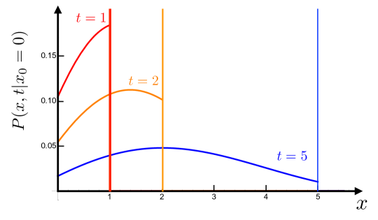
Figure 1: The density $P(x,t|x_{0}=0)$ in Eq. (43) is plotted as a function of $x$ for three different times $t=1$ (red), $t=2$ (orange) and $t=5$ (blue) with parameter values $v_{0}=1$ and $\gamma=1$ and symmetric initial conditions $b_{\pm}=1/2$. For these parameter values, the range of $x$ is over $x\in[0,t]$ and at $x=t$, there is a delta function (indicated by the colored vertical lines) with amplitude $e^{-t}/2$ which corresponds to a right moving particle which has not tumbled up to time $t$. This delta peak at $x=t$ damps down exponentially fast with time $t$ (which is sketched by a thinner vertical line as time increases).

Inserting $q_{-}(0,s)$ from Eq. (30) into Eq. (28) we get the double Laplace transform of the total probability density $P(x,t)$

$${\cal P}(p,s)={\cal P}_{+}(p,s)+{\cal P}_{-}(p,s)=\frac{\sqrt{s+2\,\gamma}}{s(s+2\gamma)-v_{0}^{2}\,p^{2}}\,\left[\sqrt{s+2\gamma}\,e^{-p\,x_{0}}-\frac{v_{0}\,p+s+2\gamma}{\sqrt{s+2\,\gamma}+\sqrt{s}}\,e^{-\sqrt{\frac{s(s+2\,\gamma)}{v_{0}^{2}}}\,x_{0}}\right]\,.$$ (36)

From this exact double Laplace transform, one can easily compute the survival probability $S(x_{0},t)$ of the RTP up to time $t$, starting from $x_{0}$. This is obtained by integrating over the final position: $S(x_{0},t)=\int_{0}^{\infty}P(x,t)\,dx$. Consequently, one gets

$$\int_{0}^{\infty}S(x_{0},t)\,e^{-s\,t}\,dt={\cal P}(p=0,s)=\frac{1}{s}\left[1-\frac{\sqrt{s+2\gamma}}{\sqrt{s+2\,\gamma}+\sqrt{s}}\,e^{-\sqrt{\frac{s(s+2\,\gamma)}{v_{0}^{2}}}\,x_{0}}\right]\,\;.$$ (37)

Interestingly, by comparing this result (37) with the result obtained before for $P(0,t|x_{0})$ in Eq. (31), we find that the first-passage probability to the origin $\partial_{t}S(x_{0},t)$ is given by

$$\partial_{t}S(x_{0},t)=-v_{0}\,P(0,t|x_{0})\;.$$ (38)

This can be understood as follows. Defining a probability current $J(x,t)$ such that $\partial_{t}P(x,t)=-\partial_{x}J(x,t)$, we see from Eqs. (13) and (14) that $J(x,t)=v_{0}[P_{+}(x,t)-P_{-}(x,t)]$. In particular, the current at $x=0$ is $J(x=0,t)=-v_{0}P_{-}(0,t)$ since $P_{+}(0,t)=0$ [see Eq. (17)]. Integrating over space, one thus has $\partial_{t}S(x_{0},t)=-[J(x,t)]_{0}^{+\infty}=J(0,t)=-v_{0}P_{-}(0,t)$, which, by further using that $P(0,t|x_{0})=P_{+}(0,t|x_{0})+P_{-}(0,t|x_{0})=P_{-}(0,t|x_{0})$, yields the relation in Eq. (38). Using the asymptotic decay of $P(0,t|x_{0})$ for large $t$ from Eq. (33) on the right hand side of Eq. (38) and integrating over $t$, we get the large $t$ decay of the survival probability $S(x_{0},t)$ for fixed $x_{0}$

$$S(x_{0},t)\simeq\frac{1}{\sqrt{\pi\,D\,t}}\,\left(x_{0}+\frac{v_{0}}{2\gamma}\right)\,;\quad\quad{\rm where}\quad D=\frac{v_{0}^{2}}{2\gamma}\,.$$ (39)

A similar result holds for more general inhomogeneous initial condition as we show later.

The result in Eq. (37) for the homogeneous initial condition coincides with the known result on survival probability that was originally deduced by using a backward Fokker-Planck approach Malakar_2018 ; EM_2018 . Here we used a forward Fokker-Planck method that gave us access to a more general quantity, namely the joint probability $P(x,t)$ that the particle survives up to $t$ and arrives at $x$ at time $t$. To the best of our knowledge, we have not come across, in the literature, the explicit double Laplace transform of the joint probability in Eq. (36). This result (36) simplifies a bit for the special initial position $x_{0}=0$

$${\cal P}(p,s|x_{0}=0)=\frac{\sqrt{s+2\gamma}}{\left(\sqrt{s+2\gamma}+\sqrt{s}\right)\,\left(v_{0}\,p+\sqrt{s(s+2\gamma)}\right)}\,.$$ (40)

Inverting trivially with respect to $p$ we get

$$\int_{0}^{\infty}P(x,t|x_{0}=0)\,e^{-s\,t}\,dt=\frac{\sqrt{s+2\gamma}}{v_{0}\,\left(\sqrt{s+2\gamma}+\sqrt{s}\right)}\,e^{-\sqrt{\frac{s(s+2\,\gamma)}{v_{0}^{2}}}\,x}\,.$$ (41)

Comparing the rhs of Eqs. (41) and (30), we notice the identity valid at all times

$$P(x,\,t|x_{0}=0)=P(0,\,t|x_{0}=x)\,,$$ (42)

which expresses the time-reversal symmetry valid in this special case of homogeneous initial condition $b_{\pm}=1/2$. Thus, for this initial condition $x_{0}=0$, we can explicitly invert the Laplace transform (as in Eq. (32)) to obtain the total probability density $P(x,t|x_{0}=0)$

$$P(x,t|x_{0}=0)=\frac{\gamma\,e^{-\gamma t}}{2v_{0}}\left[\frac{x}{x+v_{0}\,t}\,I_{0}(\rho)+\frac{1}{\rho}\left(\frac{v_{0}\,t-x}{v_{0}\,t+x}+\frac{\gamma\,x}{v_{0}}\right)\,I_{1}(\rho)\right]\,\theta(v_{0}\,t-x)+\frac{e^{-\gamma\,t}}{2}\,\delta(v_{0}\,t-x)$$

$${\rm with}\quad\rho=\frac{\gamma}{v_{0}}\sqrt{v_{0}^{2}\,t^{2}-x^{2}}\,.$$ (43)

A plot of $P(x,t|x_{0}=0)$ is provided in Fig. 1. The result in Eq. (43) can be cast in a scaling form in terms of two dimensionless scaling variables: $z=x/{(v_{0}\,t)}$ and $T=\gamma\,t$. One gets

$$P(x,t|x_{0}=0)=\frac{\gamma}{2v_{0}}\,F\left(\frac{x}{v_{0}\,t},\,\gamma\,t\right)$$ (44)

where the scaling function $F(z,T)$ is given by

$$F(z,T)=e^{-T}\left[\frac{z}{z+1}\,I_{0}\left(T\,\sqrt{1-z^{2}}\right)+\frac{1}{T\sqrt{1-z^{2}}}\left(\frac{1-z}{1+z}+z\,T\right)\,I_{1}\left(T\,\sqrt{1-z^{2}}\right)\right]\theta(1-z)+\frac{1}{2}\,e^{-T}\,\delta(1-z)\,.$$ (45)

Finally, we remark that in the diffusive limit $v_{0}\to\infty$, $\gamma\to\infty$ while keeping the ratio $v_{0}^{2}/\gamma=2\,D$ fixed, Eq. (36) reduces to

$${\cal P}(p,s)\simeq\frac{e^{-\frac{\sqrt{s}x_{0}}{\sqrt{D}}}-e^{-p\,x_{0}}}{Dp^{2}-s}\,.$$ (46)

This double transform can be easily inverted to give

$$P(x,t|x_{0})=\frac{1}{\sqrt{4\pi\,D\,t}}\,\left[e^{-(x-x_{0})^{2}/{(4\,D\,t)}}-e^{-(x+x_{0})^{2}/{(4\,D\,t)}}\right]\,.$$ (47)

This is precisely the image solution of an ordinary Brownian motion with an absorbing wall at the origin Chandra_1943 ; Redner_book ; Persistence_review . Hence, we verify that in this diffusive limit, the RTP behaves as an ordinary ‘passive’ Brownian motion with diffusion constant $D$, as expected.

Inhomogeneous initial condition. The technique used above for the homogeneous case $b_{\pm}=1/2$ generalises, in a straightforward manner, to the generic inhomogeneous initial condition with arbitrary $b_{+}$ and $b_{-}=1-b_{+}$. Without repeating the intermediate steps, we just provide the main results here. The analogue of Eq. (32) for $P(0,t|x_{0})$, for arbitrary $b_{+}$, reads

$$P(0,t|x_{0})=\frac{\gamma\,e^{-\gamma t}}{v_{0}}\left[\frac{b_{+}x_{0}}{x_{0}+v_{0}\,t}\,I_{0}(\rho)+\frac{1}{\rho}\left(b_{+}\frac{v_{0}\,t-x_{0}}{v_{0}\,t+x_{0}}+b_{-}\frac{\gamma\,x_{0}}{v_{0}}\right)\,I_{1}(\rho)\right]\,\theta(v_{0}\,t-x_{0})+b_{-}e^{-\gamma\,t}\,\delta(v_{0}\,t-x_{0})$$

$${\rm with}\quad\rho=\frac{\gamma}{v_{0}}\sqrt{v_{0}^{2}\,t^{2}-x_{0}^{2}}\,.$$ (48)

Consequently, its asymptotic behaviors for small and large $t$, for fixed $x_{0}$, are given by

$$P(0,t|x_{0})\approx\begin{cases}&b_{-}\,\delta(x_{0})\;,\quad\quad\quad\,\hskip 71.13188pt{\rm as}\quad t\to 0\\ \\ &\dfrac{1}{\sqrt{2\pi\,\gamma\,v_{0}^{2}}}\,\left(b_{+}+\dfrac{\gamma\,x_{0}}{v_{0}}\right)\,\dfrac{1}{t^{3/2}}\;,\quad{\rm as}\quad t\to\infty\,.\end{cases}$$ (49)

Note again that the first term in the large $t$ asymptotics (in the second line of Eq. (49)) is proportional to $b_{+}$, i.e., the probability that initially the RTP has a velocity $+v_{0}$.

The survival probability $S(x_{0},t)$, for general $b_{+}$, turns out to be exactly the same as in Eq. (37) for the homogeneous case, up to an overall factor $2\,b_{+}$ and we get

$$\int_{0}^{\infty}S(x_{0},t)\,e^{-s\,t}\,dt={\cal P}(p=0,s)=\frac{2\,b_{+}}{s}\left[1-\frac{\sqrt{s+2\gamma}}{\sqrt{s+2\,\gamma}+\sqrt{s}}\,e^{-\sqrt{\frac{s(s+2\,\gamma)}{v_{0}^{2}}}\,x_{0}}\right]\,\;.$$ (50)

For instance in the special case $x_{0}=0$ the Laplace inversion gives

$$S(0,t)=b_{+}e^{-\gamma t}(I_{0}(\gamma t)+I_{1}(\gamma t))$$ (51)

for $t\geq 0^{+}$, noting that $S(0,0)=1$ (by definition), but $S(0,0^{+})=1-b_{-}=b_{+}$ from Eq. (51). A similar calculation, keeping track of ${\cal P}_{+}(p,s)$ and ${\cal P}_{-}(p,s)$ separately and then inverting the Laplace transform, gives

$$S_{+}(0,t)-S_{-}(0,t)=b_{+}e^{-\gamma t}(I_{0}(\gamma t)-I_{1}(\gamma t))$$ (52)

where $S_{\pm}(0,t)$ are the survival probabilities up to time $t$ with final velocity $\pm v_{0}$ at time $t$, with $S(0,t)=S_{+}(0,t)+S_{-}(0,t)$. They satisfy $S_{+}(0,0)=b_{+}$ and $S_{-}(0,0)=b_{-}$, and $S_{+}(0,0^{+})=b_{+}$ and $S_{-}(0,0^{+})=0$. The ratio of the surviving probabilities is thus $S_{-}(0,t)/S_{+}(0,t)=I_{1}(\gamma t)/I_{0}(\gamma t)$ which is $\simeq\frac{\gamma}{2}t$ at small time and $\simeq 1-\frac{1}{2\gamma t}$ at large $t$. This is consistent with an equilibration between the two states at large time and far from the wall.

The analogue of Eq. (41), in the inhomogeneous case is

$$\int_{0}^{\infty}P(x,t|x_{0}=0)\,e^{-s\,t}\,dt=\frac{2\,b_{+}\,\sqrt{s+2\gamma}}{v_{0}\,\left(\sqrt{s+2\gamma}+\sqrt{s}\right)}\,e^{-\sqrt{\frac{s(s+2\,\gamma)}{v_{0}^{2}}}\,x}\,.$$ (53)

It turns out that the time reversal symmetry, found in Eq. (42) for the special case $b_{\pm}=1/2$, is no longer valid for generic $b_{+}\neq 1/2$.

Late time asymptotic behavior of $S(x_{0},t)$. We conclude this section with the following main observation on the late time behavior of the survival probability $S(x_{0},t)$ for generic inhomogeneous initial condition. Clearly, the relation $\partial_{t}S(x_{0},t)=-v_{0}\,P(0,t|x_{0})$ in Eq. (38) holds for generic $b_{+}$. Substituting the asymptotic large time decay of $P(0,t|x_{0})$ from Eq. (49) in this relation then provides the large $t$ decay of $S(x_{0},t)$ for fixed $x_{0}$ and $b_{+}$

$$S(x_{0},t)\simeq\frac{1}{\sqrt{\pi\,D\,t}}\,\left(x_{0}+\xi_{\rm Milne}\right)\,;\quad\quad{\rm where}\quad D=\frac{v_{0}^{2}}{2\gamma}$$ (54)

and the constant $\xi_{\rm Milne}$ is given exactly by

$$\xi_{\rm Milne}=b_{+}\,\frac{v_{0}}{\gamma}\,.$$ (55)

It is instructive to compare our result in Eq. (54) with the one for a passive Brownian particle. In the latter case, we recall from the introduction that the survival probability $S(x_{0},t)\sim x_{0}/\sqrt{\pi\,D\,t}$ at late times. In the case of the RTP, $S(x_{0},t)$ in Eq. (54) again decays with same algebraic law $t^{-1/2}$ as in the passive Brownian case with an effective diffusion constant $D=v_{0}^{2}/{2\gamma}$, but there is one important and crucial difference between the two cases. The amplitude $x_{0}$ of the power-law $t^{-1/2}$ decay in the passive case vanishes exactly at $x_{0}=0$, i.e., if the particle starts at the wall. In contrast, for the active RTP the amplitude $(x_{0}+\xi_{\rm Milne})$ approaches a nonzero constant $\xi_{\rm Milne}=b_{+}v_{0}/\gamma$ as $x_{0}\to 0$. Thus, even if the RTP starts at the wall, with a finite probability it can survive up to time $t$. Thus, the late time survival probability for the RTP is exactly of the same form as in the passive case, but with an effective diffusion constant $D=v_{0}^{2}/(2\gamma)$ and an effective initial distance from the wall $(x_{0}+\xi_{\rm Milne})$. In other words, at late times an active RTP behaves identically to a passive Brownian but with the location of the absorbing wall effectively shifted from the origin to $-\xi_{\rm Milne}=-b_{+}v_{0}/\gamma$. This effective ‘extrapolation’ length or ‘shifting of the wall’ also happens in a class of neutron scattering problems where the shift is known as the Milne extrapolation length—hence we have denoted it by $\xi_{\rm Milne}$. Similar Milne-like extrapolation lengths also emerge in certain trapping problems of discrete-time random walks MCZ_2006 ; ZMC_2007 ; MMS_2017 . Thus our main conclusion from this section is that while the exponent $1/2$ characterizing the power-law decay of $S(x_{0},t)$ is the same for both the passive Brownian and the active RTP, the fingerprint of the ‘activeness’ actually is manifest in the amplitude of this power-law decay (and not in the exponent). While an active RTP has a nonzero Milne extrapolation length $\xi_{\rm Milne}=b_{+}v_{0}/\gamma>0$, for a passive Brownian motion $\xi_{\rm Milne}=0$ identically.

III Two non-crossing RTP’s on a line

In this section we consider two independent RTP’s on a line and we are interested in computing the probability that they do not cross each other up to time $t$. As discussed in the introduction, unlike the Brownian particles, the first-passage probability for the two-RTP problem can not be reduced to that of a single RTP in the presence of an absorbing wall at the origin. In this section, we show that the first-passage probability in this non-Markovian two-RTP problem can nevertheless be fully solved, using a straightforward generalisation of our techniques developed in the previous section for a single RTP problem.

We consider two RTP’s on a line whose positions $x(t)$ (the particle on the right in Fig. 2) and $y(t)$ (the particle on the left) evolve in time independently via the Langevin equations

$$\frac{dx}{dt}=v_{0}\,\sigma_{1}(t)\,,\quad\frac{dy}{dt}=v_{0}\,\sigma_{2}(t)\,,$$ (56)

where $\sigma_{1}(t)$ and $\sigma_{2}(t)$ are two independent telegraphic noises. For simplicity, we assume that the intrinsic speed $v_{0}$, as well as the noise flipping rate $\gamma$ for both particles are the same, though our results can be straightforwardly generalised to the cases when the parameters of the two noises are different. The particles start initially at $x(0)>y(0)$. We are interested in computing the probability that the two particles do not cross each other up to time $t$ (note that they may encounter each other, but not cross each other).

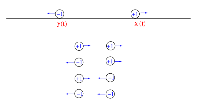
Figure 2: Two RTP’s on a line. The position of the particle on the right (left) are denoted respectively by $x(t)$ and $y(t)$, with initial positions $x(0)>y(0)$. The internal state $\sigma_{1}(t)$ and $\sigma_{2}(t)$ associated with the two particles can be in four possible configurations: $++$, $+-$, $-+$ and $--$, as shown in the figure.

We define $P_{\sigma_{1},\sigma_{2}}(x,y,t)$ as the joint probability that (i) the right particle reaches $x$ at time $t$ with internal state $\sigma_{1}$ (ii) the left particle reaches $y$ at time $t$ with internal state $\sigma_{2}$ and (iii) they do not cross each other up to $t$. There are thus four possibilities denoted respectively by $P_{++}$, $P_{+-}$, $P_{-+}$ and $P_{--}$. The total probability is obtained by summing over the internal states

$$P(x,y,t)=P_{++}(x,y,t)+P_{+-}(x,y,t)+P_{-+}(x,y,t)+P_{--}(x,y,t)\,.$$ (57)

Following the method for a single RTP, one can easily write down the Fokker-Planck equations for these probabilities

$$\partial_{t}P_{++}=-v_{0}\partial_{x}P_{++}-v_{0}\partial_{y}P_{++}-2\gamma P_{++}+\gamma(P_{+-}+P_{-+})$$ (58)

$$\partial_{t}P_{+-}=-v_{0}\partial_{x}P_{+-}+v_{0}\partial_{y}P_{+-}-2\gamma P_{+-}+\gamma(P_{++}+P_{--})$$ (59)

$$\partial_{t}P_{-+}=v_{0}\partial_{x}P_{-+}-v_{0}\partial_{y}P_{-+}-2\gamma P_{-+}+\gamma(P_{++}+P_{--})$$ (60)

$$\partial_{t}P_{--}=v_{0}\partial_{x}P_{--}+v_{0}\partial_{y}P_{--}-2\gamma P_{--}+\gamma(P_{+-}+P_{-+})\;.$$ (61)

We now introduce the non-crossing condition restricting to $x(t)>y(t)$, i.e., the process stops if the two particles cross each other. This non-crossing condition can be incorporated via the appropriate boundary condition

$$P_{+-}(x=y,t)=0\;.$$ (62)

This condition can again be deduced by considering the time evolution of a trajectory starting at $x=y$ during a small interval $dt$, and taking the $dt\to 0$, as in the single RTP case. Indeed observing the state where $x(t)$ has velocity $+v_{0}$, $y(t)$ has velocity $-v_{0}$, and $x(t)=y(t)$ necessarily means that the two particles have crossed before $t$, which is not allowed. Once again, as we show below, this single boundary condition at $x=y$, along with the Dirichlet boundary conditions as $x\to\infty$ and $y\to-\infty$, are sufficient to uniquely determine the solution to the Fokker-Planck equations (61). We can work with general initial conditions, but for simplicity we set $x(0)=z_{0}$ and $y(0)=-z_{0}$, equidistant from the origin on opposite sides. The initial condition is given by

$$P_{\sigma_{1},\sigma_{2}}(x,y,t=0)=\left(b_{++},b_{+-},b_{-+},b_{--}\right)\,\delta\left(\frac{x-y}{2}-z_{0}\right)\delta\left(\frac{x+y}{2}\right)$$ (63)

where the $b_{\pm\pm}$ denote the initial probabilities of the $4$ internal state configurations, with $b_{++}+b_{+-}+b_{-+}+b_{--}=1$.

To solve these equations (61), it is convenient to go to the center of mass and relative coordinates, i.e., we make the change of variables

$$w=\frac{x+y}{2}\quad,\quad z=\frac{x-y}{2}\;.$$ (64)

In this new pair of coordinates the probability $P_{\sigma_{1},\sigma_{2}}(x,y,t)$ is a different function of $w$ and $z$. But to avoid explosion of new symbols and with a slight abuse of notations, we will continue to denote it by $P$, i.e., by $P_{\sigma_{1},\sigma_{2}}(w,z,t)$. Then Eqs. (61) become

$$\partial_{t}P_{++}=-v_{0}\partial_{w}P_{++}-2\gamma P_{++}+\gamma(P_{+-}+P_{-+})$$ (65)

$$\partial_{t}P_{+-}=-v_{0}\partial_{z}P_{+-}-2\gamma P_{+-}+\gamma(P_{++}+P_{--})$$ (66)

$$\partial_{t}P_{-+}=v_{0}\partial_{z}P_{-+}-2\gamma P_{-+}+\gamma(P_{++}+P_{--})$$ (67)

$$\partial_{t}P_{--}=v_{0}\partial_{w}P_{--}-2\gamma P_{--}+\gamma(P_{+-}+P_{-+})$$ (68)

Note that the center of mass $w(t)$ can be any real number (positive or negative), but the relative coordinate $z(t)>0$ is in the positive half-space, starting from the initial value $z_{0}>0$. The boundary condition (62) now translates into

$$P_{+-}(w,z=0,t)=0\,.$$ (69)

To proceed, we first define Fourier-Laplace transforms in space

$${\tilde{P}}_{\sigma_{1},\sigma_{2}}(k,p,t)=\int_{-\infty}^{\infty}dw\,\int_{0}^{\infty}dz\,e^{-i\,k\,w}\,e^{-p\,z}\,P_{\sigma_{1},\sigma_{2}}(w,z,t)\,.$$ (70)

Furthermore, we will also take the Laplace transform with respect to time and define

$${\cal P}_{\sigma_{1},\sigma_{2}}(k,p,s)=\int_{0}^{\infty}dt\,e^{-s\,t}\,{\tilde{P}}_{\sigma_{1},\sigma_{2}}(k,p,t)\,.$$ (71)

Taking these Fourier-Laplace transforms of Eq. (68) and using the boundary condition (69) we get

$$s{\cal P}_{++}-{\tilde{P}}_{++}(k,p,t=0)=i\,v_{0}\,k\,{\cal P}_{++}-2\gamma{\cal P}_{++}+\gamma({\cal P}_{+-}+{\cal P}_{-+})$$ (72)

$$s{\cal P}_{+-}-{\tilde{P}}_{+-}(k,p,t=0)=-v_{0}\,p\,{\cal P}_{+-}-2\gamma{\cal P}_{+-}+\gamma({\cal P}_{++}+{\cal P}_{--})$$ (73)

$$s{\cal P}_{-+}-{\tilde{P}}_{-+}(k,p,t=0)=v_{0}p{\cal P}_{-+}-v_{0}\,q_{-+}(k,0,s)-2\gamma{\cal P}_{-+}+\gamma({\cal P}_{++}+{\cal P}_{--})$$ (74)

$$s{\cal P}_{--}-{\tilde{P}}_{--}(k,p,t=0)=-i\,v_{0}\,k\,{\cal P}_{--}-2\gamma{\cal P}_{--}+\gamma({\cal P}_{+-}+{\cal P}_{-+})\;,$$ (75)

where we have defined

$$q_{-+}(k,0,s)=\int_{0}^{\infty}dt\,e^{-s\,t}\,\int_{-\infty}^{\infty}dw\,e^{-i\,k\,w}\,P_{-+}(w,z=0,t)\,$$ (76)

which still remains unknown and will be self-consistently determined using the pole-cancelling mechanism as in the single RTP case. Note that the initial condition in Eq. (63) implies, putting $t=0$ in Eq. (70),

$${\tilde{P}}_{\sigma_{1},\sigma_{2}}(k,p,t=0)=e^{-p\,z_{0}}\,\left(b_{++},b_{+-},b_{-+},b_{--}\right)\,.$$ (77)

Substituting the initial condition (77) on the left hand side (lhs) of Eq. (75) and inverting the $4\times 4$ matrix gives

$${\cal P}_{\sigma_{1},\sigma_{2}}(k,p,s)$$ (78)

$$=\begin{pmatrix}-v_{0}ik+2\gamma+s&-\gamma&-\gamma&0\\ -\gamma&v_{0}p+2\gamma+s&0&-\gamma\\ -\gamma&0&-v_{0}p+2\gamma+s&-\gamma\\ 0&-\gamma&-\gamma&v_{0}ik+2\gamma+s\end{pmatrix}^{-1}\left(\begin{pmatrix}0\\ 0\\ -v_{0}q_{-+}(k,z=0,s)\\ 0\end{pmatrix}+e^{-pz_{0}}\begin{pmatrix}b_{++}\\ b_{+-}\\ b_{-+}\\ b_{--}\end{pmatrix}\right)\;.$$

After inverting the $4\times 4$ matrix using Mathematica, we obtain ${\cal P}_{\sigma_{1},\sigma_{2}}(k,p,s)$ explicitly. The resulting expressions are too long to display and are not very illuminating. Summing over the internal states, the Fourier-Laplace transform of the total probability density is given by

$${\cal P}(k,p,s)={\cal P}_{++}(k,p,s)+{\cal P}_{+-}(k,p,s)+{\cal P}_{-+}(k,p,s)+{\cal P}_{--}(k,p,s)\,.$$ (79)

But even this expression is too long for arbitrary initial conditions. Hence we just present the result for the fully symmetric case $b_{++}=b_{+-}=b_{-+}=b_{--}=\frac{1}{4}$ which is a bit simpler, and restore the general $b_{\sigma_{1},\sigma_{2}}$ in some of the final results.

For this symmetric initial condition $b_{++}=b_{+-}=b_{-+}=b_{--}=\frac{1}{4}$, we get

$${\cal P}(k,p,s)$$ (80)

$$=\frac{e^{-pz_{0}}\left((2\gamma+s)\left(v_{0}^{2}(k-p)(k+p)+2(2\gamma+s)(4\gamma+s)\right)-2v_{0}e^{pz_{0}}q_{-+}(k,0,s)\left(k^{2}v_{0}^{2}+(2\gamma+s)(4\gamma+s)\right)\left(2\gamma+pv_{0}+s\right)\right)}{2\left(-k^{2}p^{2}v_{0}^{4}+v_{0}^{2}(k-p)(k+p)(2\gamma+s)^{2}+s(2\gamma+s)^{2}(4\gamma+s)\right)}$$

To fix the unknown $q_{-+}(k,0,s)$, we look for the poles of the rhs of Eq. (80) in the complex $p$ plane. They are located at

$$p^{*}_{\pm}=\pm\frac{(2\gamma+s)\sqrt{k^{2}v_{0}^{2}+s^{2}+4\gamma s}}{v_{0}\sqrt{k^{2}v_{0}^{2}+(2\gamma+s)^{2}}}\;.$$ (81)

Using the pole-cancelling argument as in the previous section, the numerator of the rhs in Eq. (80) must vanish at the positive pole $p^{*}_{+}$. This leads to a long but explicit formula for the unknown $q_{-+}(k,0,s)$

$$q_{-+}(k,0,s)=\frac{\left(k^{2}v_{0}^{2}+(2\gamma+s)(4\gamma+s)\right)\exp\left(-\frac{z_{0}(2\gamma+s)\sqrt{k^{2}v_{0}^{2}+s(4\gamma+s)}}{v_{0}\sqrt{k^{2}v_{0}^{2}+(2\gamma+s)^{2}}}\right)}{2v_{0}\left(\sqrt{k^{2}v_{0}^{2}+(2\gamma+s)^{2}}\sqrt{k^{2}v_{0}^{2}+s(4\gamma+s)}+k^{2}v_{0}^{2}+(2\gamma+s)^{2}\right)}\;.$$ (82)

A similar but more complicated expression for $q_{-+}(k,0,s)$ can be obtained explicitly for the inhomogeneous initial condition (with arbitrary $b_{\sigma_{1},\sigma_{2}}$), but we do not display it here. Note from the definition (76) that $q_{-+}(k,0,s)$ is just the Fourier-Laplace transform of $P_{-+}(w,z=0,t)$. In addition, if we set $k=0$ in Eq. (76), i.e., we integrate over the center of mass coordinate $w$, we get

$$q_{-+}(0,0,s)=\int_{0}^{\infty}dt\,e^{-s\,t}\,\int_{-\infty}^{\infty}dw\,P_{-+}(w,z=0,t)\,.$$ (83)

The quantity $\int_{-\infty}^{\infty}dw\,P_{-+}(w,z=0,t)$ has the dimension of the inverse length and is proportional to the probability of ‘reaction’ or ‘encounter’ of the two particles in the state $(-+)$ at time $t$ without crossing each other for all $0\leq t^{\prime}<t$, starting at an initial separation $2z_{0}$. In fact, one can define an encounter probability density at time $t$ (with the dimension of the inverse time) as

$$p_{\rm enc}(t|z_{0})=v_{0}\,\int_{-\infty}^{\infty}dw\,P_{-+}(w,z=0,t)\,.$$ (84)

This nonzero ‘encountering’ probability is a typical hallmark of active particles—it strictly vanishes for passive Brownian particles. Our analysis thus gives access to this nontrivial encountering probability. Setting $k=0$ in Eq. (82), or more generally in the counterpart of Eq. (82) for arbitrary $b_{\sigma_{1},\sigma_{2}}$, we get ( thus restoring the dependence on the initial probabilities)

$$\int_{0}^{\infty}p_{\rm enc}(t|x_{0})\,e^{-st}\,dt=v_{0}\,q_{-+}(0,0,s)=\frac{(2\gamma+(b_{-+}+b_{+-})s+(b_{-+}-b_{+-})\sqrt{s(4\gamma+s)})e^{-\frac{\sqrt{s(4\gamma+s)}}{v_{0}}\,z_{0}}}{\left(s+2\gamma+\sqrt{s}\sqrt{4\gamma+s}\right)}\,.$$ (85)

Note that $\int_{0}^{\infty}p_{\rm enc}(t|z_{0})\,dt=1$ and hence $p_{\rm enc}(t|z_{0})$ has the interpretation of a probability density of encounter between time $t$ and $t+dt$, starting from $z_{0}$. Remarkably, this Laplace transform can be inverted exactly for all $t$ (see Appendix B). The solution can be conveniently expressed at all times $t$ in a scaling form

$$p_{\rm enc}(t|z_{0})=\gamma\,G\left(\frac{2\gamma\,z_{0}}{v_{0}}\,,2\,\gamma\,t\right)$$ (86)

where the scaling function $G(y,T)$ is given exactly by

$$G(y,T)=2e^{-T}\bigg{[}b_{-+}\,\delta(T-y)+\frac{1}{y+T}\left(2b_{+-}\frac{T-y}{T+y}+(b_{++}+b_{--})y\right)\,I_{0}(\rho)$$

$$+\frac{1}{\rho}\left(y(b_{-+}+b_{+-})+(b_{++}+b_{--})\frac{T-y}{T+y}-2b_{+-}\frac{1}{T+y}\left(y^{2}+\frac{2(T-y)}{T+y}\right)\right)\,I_{1}(\rho)\bigg{]}\theta(T-y)\;,$$ (87)

where $\rho=\sqrt{T^{2}-y^{2}}$. In Fig. 3 we show a plot of $p_{\rm enc}(t|z_{0})$, given in Eqs. (86) and (87), for $b_{\pm\pm}=1/4$, as a function of $t$ and for two different values of $z_{0}$. Note that $p_{\rm enc}(t|z_{0})=0$ for $t<z_{0}/v_{0}$ since $z_{0}/v_{0}$ is the minimal time needed for the two particles to encounter (this corresponds to pairs ($-+$) whose velocities have not changed up to that time). The limiting behavior of $p_{\rm enc}(t|z_{0})$ when $t\to(z_{0}/v_{0})^{+}$ can be obtained from the explicit expression (87). It has both a singular part $\propto\delta(t-z_{0}/v_{0})$ as well as a regular finite part (see Fig. 3) and reads

$$p_{\rm enc}(t|z_{0})\to b_{-+}\,e^{-\frac{2\gamma z_{0}}{v_{0}}}\delta\left(t-\frac{z_{0}}{v_{0}}\right)+2\gamma e^{-\frac{2\gamma z_{0}}{v_{0}}}\left(\frac{b_{++}+b_{--}}{2}+\frac{\gamma z_{0}}{v_{0}}b_{-+}\right)\;,\;\;\;t\to(z_{0}/v_{0})^{+}\;.$$ (88)

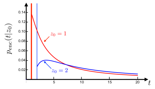
Figure 3: Plot of $p_{\rm enc}(t|z_{0})$, as given in Eqs. (86) and (87) as a function of $t$ and for two different values of $z_{0}=1$ (red) and $z_{0}=2$ (blue) with parameter values $v_{0}=1$ and $\gamma=1$ and symmetric initial conditions $b_{\pm\pm}=1/4$. The vertical colored lines correspond to the delta-function in Eqs. (87) and (88) at $t=z_{0}$, whose weight decreases exponentially with $z_{0}$. These correspond to pairs $(-+)$ which have not changed their velocities up to time $t=z_{0}/v_{0}$.

The large $t$ behavior of $p_{\rm enc}(t|z_{0})$ for fixed $z_{0}$ can be easily obtained by analysing the small $s$ behavior of $q_{-+}(0,0,s)$. Taking the small $s$ limit on the rhs of Eq. (85) we get

$$v_{0}\,q_{-+}(0,0,s)=1-\frac{1}{\sqrt{\gamma}}\,\left(1+b_{+-}-b_{-+}+\frac{2\gamma}{v_{0}}\,z_{0}\right)\,\sqrt{s}+O(s)\,.$$ (89)

Consequently, upon inverting and using a Tauberian theorem, we find that the encountering probability at late times decays algebraically as

$$p_{\rm enc}(t|z_{0})\approx\frac{1}{\sqrt{{4\pi\gamma}}}\left(1+b_{+-}-b_{-+}+\frac{2\gamma}{v_{0}}\,z_{0}\right)\,\frac{1}{t^{3/2}}\,.$$ (90)

The same result also follows from the exact form in Eq. (87). Extending the calculation to obtain the encounter probabilities associated to the pairs $(++)$ and $(--)$, i.e. $\int_{-\infty}^{+\infty}dw\,P_{++}(w,z=0,t)$ and $\int^{+\infty}_{-\infty}dw\,P_{--}(w,z=0,t)$, we find that at large time they both decay as $t^{-3/2}$ with the same amplitude as $p_{\rm enc}(t|z_{0})$ up to a factor $1/2$, i.e. both quantities are equivalent to $\frac{1}{2}p_{\rm enc}(t|z_{0})$ for large time $t$.

Substituting the exact $q_{-+}(k,0,s)$ from Eq. (82) into (80) finally gives (for $b_{\pm\pm}=1/4$)

$${\cal P}(k,p,s)=$$ (91)

$$\frac{e^{-pz_{0}}\left((2\gamma+s)\left(v_{0}^{2}(k-p)(k+p)+2(2\gamma+s)(4\gamma+s)\right)-\frac{\left(k^{2}v_{0}^{2}+(2\gamma+s)(4\gamma+s)\right){}^{2}\left(2\gamma+pv_{0}+s\right)\exp\left(z_{0}\left(p-\frac{(2\gamma+s)\sqrt{k^{2}v_{0}^{2}+s^{2}+4\gamma s}}{v_{0}\sqrt{k^{2}v_{0}^{2}+(2\gamma+s)^{2}}}\right)\right)}{\sqrt{k^{2}v_{0}^{2}+s^{2}+4\gamma s}\sqrt{k^{2}v_{0}^{2}+(2\gamma+s)^{2}}+k^{2}v_{0}^{2}+(2\gamma+s)^{2}}\right)}{2\left(-k^{2}p^{2}v_{0}^{4}+v_{0}^{2}(k-p)(k+p)(2\gamma+s)^{2}+s(2\gamma+s)^{2}(4\gamma+s)\right)}$$

This rather long (albeit explicit) expression simplifies a bit by setting $k=0$, i.e., integrating over the center of mass coordinate

$${\cal P}(k=0,p,s)=\frac{e^{-pz_{0}}}{2(2\gamma+s)\left(-p^{2}v_{0}^{2}+s^{2}+4\,\gamma\,s\right)}\,\left[-p^{2}v_{0}^{2}+2\,(2\gamma+s)\,(4\gamma+s)-\frac{(2\gamma+v_{0}\,p+s)(4\gamma+s)^{2}}{2\gamma+s+\sqrt{s(s+4\gamma)}}\,e^{z_{0}\,\left(p-\frac{\sqrt{s(s+4\gamma)}}{v_{0}}\right)}\right]\,.$$ (92)

It behaves as $e^{-pz_{0}}/s$ at large $s$, consistent with the initial condition. From this exact formula (92) one can also check that $\int_{-\infty}^{+\infty}dw\,P(w,z=0,t)\simeq 2\,p_{\rm enc}(t|z_{0})$, for $t\gg 1$, which is fully consistent with our previous results mentioned below Eq. (90).

Finally, the survival probability $S(z_{0},t)$, i.e., the probability that the two particles, starting initially at a separation $z_{0}$, does not cross each other up to time $t$ is obtained by integrating over all $z$, i.e., by setting $p=0$ in Eq. (92). We get (restoring the dependence in the initial probabilities)

$$\int_{0}^{\infty}S(z_{0},t)\,e^{-s\,t}\,dt={\cal P}(k=0,p=0,s)=\frac{1}{s}\left[1-\frac{(4\gamma+2(b_{-+}+b_{+-})s+2(b_{-+}-b_{+-})\sqrt{s(4\gamma+s)})}{2\,(2\gamma+s+\sqrt{s(s+4\gamma)})}\,e^{-\frac{\sqrt{s(s+4\gamma)}}{v_{0}}\,z_{0}}\right]\,.$$ (93)

Interestingly, by comparing this relation (93) with the result obtained above for the encounter probability $p_{\rm enc}(t|z_{0})$ in Eq. (85), we find the following identity

$$\partial_{t}S(z_{0},t)=-p_{\rm enc}(t|z_{0})\;,$$ (94)

which is analogous to the identity found in Eq. (38) for the case of a single particle with an absorbing wall at the origin. As above [see the discussion below Eq. (38)], (94) can be obtained by summing all four equations in (68) and integrating for $w\in]-\infty,\infty[$ and $z\in[0,+\infty[$. This identity clearly shows that $p_{\rm enc}(t|z_{0})dt$ is the probability that the two particles encounter in the state $(-+)$, and hence die immediately, in the time interval $[t,t+dt[$. It is thus the first and last encounter of the two particles in the state $(-+)$. Again, we emphasize that this relation (94) is a specific feature of active particles, which does not hold for passive (i.e. Brownian) ones. Indeed, for Brownian particles, the encounter probability is strictly zero, while the first-passage probability is not, since the probability current at $z=0$ is non-zero.

The relation (94), together with the scaling form for the encounter probability (86), leads to the following explicit result for the survival probability

$$S(z_{0},t)=H\left(\frac{2\gamma\,z_{0}}{v_{0}}\,,2\,\gamma\,t\right)\quad,\quad\partial_{T}H(y,T)=-\frac{1}{2}G(y,T)$$ (95)

where $G(y,T)$ is given explicitly in (87). In the special case $z_{0}=0$ we obtain explicitly

$$S(0,t)=e^{-2\gamma t}\left((1+b_{+-}-b_{-+})\left(I_{0}(2\gamma t)+I_{1}(2\gamma t)\right)-\frac{b_{+-}}{\gamma t}I_{1}(2\gamma t)\right)\;,\;t>0\;.$$ (96)

Its asymptotic behaviors are easily obtained as $S(0,t)\to(1-b_{-+})$ for $t\to 0^{+}$, as expected since between $t=0$ and $t=0^{+}$ the pairs $-+$ necessarily annihilate, while $S(0,t)\approx(1+b_{+-}-b_{-+})/\sqrt{\pi\gamma t}$ for $t\to\infty$.

For arbitrary $z_{0}>0$, one can easily extract the late time behavior of $S(z_{0},t)$ from the Laplace transform in Eq. (93). Indeed, expanding for small $s$ gives

$${\cal P}(k=0,p=0,s)=\frac{v_{0}(1+b_{+-}-b_{-+})+2\gamma z_{0}}{\sqrt{\gamma}\sqrt{s}v_{0}}+O(1)\;.$$ (97)

Inverting we obtain the large time decay of the no-crossing probability

$$S(z_{0},t)\simeq\frac{v_{0}(1+b_{+-}-b_{-+})+2\gamma z_{0}}{\sqrt{\pi\,v_{0}^{2}\,\gamma\,t}}\,,$$ (98)

which is consistent with the result obtained above for $z_{0}=0$ in Eq. (96). Let us rewrite Eq. (98) as

$$S(z_{0},t)\simeq\frac{1}{\sqrt{\pi\,D^{\prime}\,t}}\left(z_{0}+\xi_{\rm Milne}\right)\,;\quad\quad{\rm where}\quad D^{\prime}=\frac{v_{0}^{2}}{4\gamma}\,,$$ (99)

and the Milne extrapolation length $\xi_{\rm Milne}$ for this two RTP problem is given by

$$\xi_{\rm Milne}=\frac{v_{0}}{2\gamma}\,(1+b_{+-}-b_{-+})\,.$$ (100)

Thus the survival probability (i.e., the probability of no crossing of the two independent RTP’s) decays as $t^{-1/2}$ at late times, as in the case of two independent ‘passive’ Brownian particles. However, the amplitude of the decay carries an interesting feature, as in the case of a single RTP in the presence of a wall. As discussed in the introduction, for two independent passive Brownian motions starting at an initial sepration $2z_{0}$, the probability of no zero crossing up to time $t$ decays at late times as $\sim z_{0}/\sqrt{\pi\,D^{\prime}\,t}$ where $D^{\prime}=D/2$ (see Eq. (4)). Thus, if $z_{0}=0$, the Brownian particles cross immediately. Hence the amplitude of the $t^{-1/2}$ decay vanishes at the absorbing boundary. In contrast, we see from Eq. (99) that in the active case, the amplitude $z_{0}+\xi_{\rm Milne}$ does not vanish when $z_{0}=0$. This is because even if the two particles start at the same initial position, with a finite probability they can go away from each other in the opposite direction and hence survive without crossing each other. The dependence of this amplitude in the initial probabilities can be understood qualitatively: (i) changing $b_{++}$ or $b_{--}$ only affects the motion of the center of mass, hence these probabilities do not appear in the survival probability (ii) to survive till late times it is clearly advantageous to start in the configuration $(+-)$ rather than in $(-+)$. In fact, the amplitude of the late time decay vanishes, when extrapolated to the negative side, at $z_{0}=-v_{0}(1+b_{+-}-b_{-+})/{2\gamma}=-\xi_{\rm Milne}$, as in the case of a single RTP in the presence of a wall. Clearly, in the passive limit $\gamma\to\infty$, the Milne extrapolation length vanishes. Hence, for two active particles also, a finite Milne extrapolation length is a clear signature of ‘activeness’ of the RTP’s dynamics.

Finally, if we take the scaling (diffusive) limit corresponding to $s\to 0$, $z_{0}\to\infty$ but keeping $\sqrt{s}z_{0}$ fixed, one finds

$${\cal P}(k=0,p=0,s)\simeq\frac{1-e^{-\frac{2\sqrt{\gamma}\sqrt{s}z_{0}}{v_{0}}}}{s}\;.$$ (101)

This Laplace transform can be easily inverted to obtain, in real time,

$$S(z_{0},t)\simeq\text{erf}\left(\frac{\sqrt{\gamma}z_{0}}{\sqrt{t}v_{0}}\right)\;,$$ (102)

which is the survival probability of a Brownian walker with diffusion constant $D^{\prime}=v_{0}^{2}/(4\gamma)$. Alternatively, one can keep $z_{0}$ fixed, but take the limit $v_{0}\to\infty$, $\gamma\to\infty$ with the ratio $D^{\prime}=v_{0}^{2}/{(4\gamma)}$ fixed. In this case, once again we recover the passive Brownian behavior as expected.

IV Conclusion

In this paper we have studied non crossing probabilities for active particles, in the framework of a simple run and tumble model with velocities $\pm v_{0}$ subjected to a telegraphic noise. We have computed explicitly the probability of non-crossing of two active RTP’s up to time $t$.

We found useful to first consider the case of a single particle with an absorbing wall. For that problem we have calculated explicitly the total probability density $P(x,t|x_{0})$ that the particle, starting at $x_{0}$ at time $t=0$, survives up to time $t$ and that it is at position $x$ at $t$. Contrarily to the passive Brownian particle (which is recovered for $v_{0}\sim\sqrt{\gamma}\to+\infty$) the probability of presence at the wall does not vanish and we found that it decreases as $t^{-3/2}$. Integration of $P(x,t|x_{0})$ over $x$ then allows to recover the survival probability $S(x_{0},t)$ obtained previously using different methods in Malakar_2018 ; EM_2018 . Here we showed an interesting exact relation for active RTP dynamics: the probability to find the particle at the wall is (minus) the time derivative of the survival probability. The latter decays at large time as $t^{-1/2}$. The amplitude of the decay of the survival probability explicitly depends on $x_{0}$ and $b_{+}$, where $b_{\pm}$ are the probabilities $b_{\pm}$ that the particle is in states $\pm v_{0}$ at time $t=0$. This defines a length scale analogous to the so called “Milne length”, known from the neutron-scattering literature.

We then studied the case of two indepedent RTP’s and computed the probability that they do not cross each other up to time $t$. In the case of two passive Brownian particles this problem can be mapped exactly to the one of the single particle with an absorbing wall. For the active problem this equivalence fails. By considering all four states for the two particle systems we obtain the double Laplace transform of the probability that the two particles, initially separated by a distance $2z_{0}>0$, have survived up to time $t$ and are at a distance $2z$ from each other at time $t$. From it we have extracted the ”encounter” probability, i.e., the probability that the two particles are at the same position at time $t$. At variance with the passive (Brownian) case it is non zero. It decays at large time as $t^{-3/2}$ with an amplitude which depends on $z_{0}$ and on the probabilities of the velocities in the initial state. Similarly to the absorbing wall problem, the encounter probability is the time derivative of the survival probability. The survival probability thus again decays at large time as $t^{-1/2}$ with an amplitude that is proportional to $(z_{0}+\xi_{\rm Milne})$. This amplitude thus vanishes when the initial $z_{0}$ is extrapolated to the negative side at $z_{0}=-\xi_{\rm Milne}$. We have computed exactly $\xi_{\rm Milne}$ for this two RTP problem. Our main conclusion is that the amplitude of the $t^{-1/2}$ decay of the late time survival probability carries a fingerprint of the activeness of the particles: active particles have a finite Milne extrapolation length $\xi_{\rm Milne}$, while the passive ones have $\xi_{\rm Milne}=0$.

In this work, we have considered the case of two “free” annihilating RTP’s. A natural question is to understand what happens if instead these particles are confined by an external potential, a situation that has recently attracted much attention for active particles Dhar_18 ; Basu_18 ; Sevilla_19 ; Dhar_2019 . Another natural question is whether there exists extensions of the so-called Karlin-McGregor formula KMG , valid for passive Brownian particles, which would allow to study an arbitrary number of non-crossing RTPs on the line. This is left for future investigations.

Appendix A Laplace inversion of Eq. (31)

To invert the Laplace transform in Eq. (31), it is useful to re-write the rhs of Eq. (31) as follows

$$\int_{0}^{\infty}P(0,t|x_{0})\,e^{-s\,t}\,dt=\frac{s+2\gamma-\sqrt{s(s+2\gamma)}}{2v_{0}\gamma}\,e^{-\sqrt{\frac{s(s+2\,\gamma)}{v_{0}^{2}}}\,x_{0}}\,.$$ (103)

In order to bring it to a more amenable form, it is convenient to rescale $t\to t/\gamma$ and $s\to\gamma\,s$ and re-express Eq. (103) as

$$\int_{0}^{\infty}P\left(0,\frac{t}{\gamma}\big{|}x_{0}\right)\,e^{-s\,t}\,dt=\frac{\gamma}{2v_{0}}\,\left[s+2-\sqrt{s(s+2)}\right]\,e^{-\sqrt{s(s+2)}\,z}\,;\quad{\rm where}\,\,z=\frac{\gamma x_{0}}{v_{0}}\;.$$ (104)

We denote by ${\cal L}_{s}^{-1}$ the inverse Laplace transform with respect to $s$. Then we invert Eq. (104) and split the rhs into two separate terms

$$P\left(0,\frac{t}{\gamma}\big{|}x_{0}\right)=\frac{\gamma}{2v_{0}}\,\left({\cal L}_{s}^{-1}\left[\left(s+1-\sqrt{s(s+2)}\right)\,e^{-\sqrt{s(s+2)}\,z}\right]+{\cal L}_{s}^{-1}\left[e^{-\sqrt{s(s+2)}\,z}\right]\right)\,.$$ (105)

The reason behind the splitting of the rhs into two terms is as follows. The Laplace inversion of the second term is known explicitly (see e.g. Ref. Malakar_2018 )

$${\cal L}_{s}^{-1}\left[e^{-\sqrt{s(s+2)}z}\right]=\frac{z\,e^{-t}}{\sqrt{t^{2}-z^{2}}}\,I_{1}\left(\sqrt{t^{2}-z^{2}}\right)\ \theta(t-z)+e^{-t}\,\delta(t-z)\,,$$ (106)

where $I_{1}(x)$ is the modified Bessel function and $\theta(x)$ is the standard Heaviside theta function. The inversion of the first term in Eq. (105) requires a bit more work. To proceed, we make use of another interesting Laplace inversion that was found in Ref. Malakar_2018

$${\cal L}_{s}^{-1}\left[\frac{s+1-\sqrt{s(s+2)}}{\sqrt{s(s+2)}}\,e^{-\sqrt{s(s+2)}\,z}\right]=e^{-t}\,\sqrt{\frac{t-z}{t+z}}\,I_{1}\left(\sqrt{t^{2}-z^{2}}\right)\,\theta(t-z)\,.$$ (107)

We then take the derivative with respect to $z$ in Eq. (107) and use the identity satisfied by the Bessel function: $x\,dI_{1}(x)/dx+I_{1}(x)=x\,I_{0}(x)$. After a few steps of straightforward algebra we get

$${\cal L}_{s}^{-1}\left[\left(s+1-\sqrt{s(s+2)}\right)\,e^{-\sqrt{s(s+2)}\,z}\right]=\frac{e^{-t}}{t+z}\left[z\,I_{0}\left(\sqrt{t^{2}-z^{2}}\right)+\sqrt{\frac{t-z}{t+z}}\,I_{1}\left(\sqrt{t^{2}-z^{2}}\right)\right]\,\theta(t-z)\,.$$ (108)

Adding Eqs. (106) and (108) on the rhs of Eq. (105) and substituting $t/\gamma\to t$ and $z=\gamma x_{0}/v_{0}$, we obtain the result in Eq. (32).

Appendix B Laplace inversion of Eq. (85)

To invert the Laplace transform in Eq. (85), we first make a change of variables $t\to t^{\prime}/{2\gamma}$ and $s\to 2\gamma\,s$ giving

$${\int_{0}^{\infty}p_{\rm enc}\left(\frac{t}{2\gamma}|z_{0}\right)e^{-st}\,dt}=2\gamma\,\frac{s(b_{-+}+b_{+-})+1+(b_{-+}-b_{+-})\sqrt{s(s+2)}}{s+1+\sqrt{s(s+2)}}\,e^{-\sqrt{s(s+2)}\,y}\,,\quad{\rm where}\quad y=\frac{2\gamma z_{0}}{v_{0}}\,.$$ (109)

Inverting and expressing $s+2=s+1+\sqrt{s(s+2)}+1-\sqrt{s(s+2)}$, we split the rhs into $3$ terms

$$p_{\rm enc}\left(\frac{t}{2\gamma}|z_{0}\right)=\; 2\gamma\,\Bigg{(}(b_{-+}+b_{+-}){\cal L}_{s}^{-1}\left[e^{-\sqrt{s(s+2)}\,y}\right]+(1-b_{-+}-b_{+-}){\cal L}_{s}^{-1}\left[\frac{1}{s+1+\sqrt{s(s+2)}}\,e^{-\sqrt{s(s+2)}\,y}\right]$$ (111)

$$-2b_{+-}{\cal L}_{s}^{-1}\left[\frac{\sqrt{s(s+2)}}{s+1+\sqrt{s(s+2)}}\,e^{-\sqrt{s(s+2)}\,y}\right]\Bigg{)}\,.$$

The first term on the rhs can be inverted explicitly using Eq. (106). The second term can be written as

$${\cal L}_{s}^{-1}\left[\frac{1}{s+1+\sqrt{s(s+2)}}\,e^{-\sqrt{s(s+2)}\,y}\right]={\cal L}_{s}^{-1}\left[\left(s+1-\sqrt{s(s+2)}\right)\,e^{-\sqrt{s(s+2)}\,y}\right]$$ (112)

and subsequently can be inverted explicitly using Eq. (108). Finally, the third term in Eq. (111) is just the derivative with respect to $y$ of the second term. Hence, one can also invert it explicitly by taking derivative of Eq. (108) with respect to $z$ and setting $z=y$. Finally, after summing up the three contributions and using the Bessel function relations, $dI_{0}(z)/dz=I_{1}(z)$ and $dI_{1}(z)/dz=I_{0}(z)-I_{1}(z)/z$, we arrive at the result in Eqs. (86) and (87).

Appendix C Some useful Laplace inversions

In this appendix we provide a list of Laplace inversions that are not easy to find in the standard literature and Mathematica is unable to find them. We believe that these inversions would be useful for future works on active systems where such Laplace transforms occur frequently. We define ${\cal L}_{s}^{-1}$ as the inverse Laplace transform of a function whose argument is denoted by $t$, i.e., $s$ is conjugate to $t$. Then the following results are true, and one can easily verify them numerically. Below we assume that $z>0$.

$${\cal L}_{s}^{-1}\left[e^{-\sqrt{s(s+2)}\,z}\right]=\frac{z\,e^{-t}}{\sqrt{t^{2}-z^{2}}}\,I_{1}\left(\sqrt{t^{2}-z^{2}}\right)\ \theta(t-z)+e^{-t}\,\delta(t-z)\,,$$ (113)

$${\cal L}_{s}^{-1}\left[\frac{1}{\sqrt{s(s+2)}}\,e^{-\sqrt{s(s+2)}\,z}\right]=e^{-t}\,I_{0}\left(\sqrt{t^{2}-z^{2}}\right)\,\theta(t-z)\,.$$ (114)

$${\cal L}_{s}^{-1}\left[\frac{s+1-\sqrt{s(s+2)}}{\sqrt{s(s+2)}}\,e^{-\sqrt{s(s+2)}\,z}\right]=e^{-t}\,\sqrt{\frac{t-z}{t+z}}\,I_{1}\left(\sqrt{t^{2}-z^{2}}\right)\,\theta(t-z)\,.$$ (115)

$${\cal L}_{s}^{-1}\left[\left(s+1-\sqrt{s(s+2)}\right)\,e^{-\sqrt{s(s+2)}\,z}\right]=\frac{e^{-t}}{t+z}\left[z\,I_{0}\left(\sqrt{t^{2}-z^{2}}\right)+\sqrt{\frac{t-z}{t+z}}\,I_{1}\left(\sqrt{t^{2}-z^{2}}\right)\right]\,\theta(t-z)\,.$$ (116)

$${\cal L}_{s}^{-1}\left[\frac{\sqrt{s(s+2)}}{s+1+\sqrt{s(s+2)}}\,e^{-\sqrt{s(s+2)}\,z}\right]$$

$$=\frac{e^{-t}}{t+z}\,\left[\frac{1}{\sqrt{t^{2}-z^{2}}}\left(z^{2}+\frac{2(t-z)}{t+z}\right)I_{1}\left(\sqrt{t^{2}-z^{2}}\right)-\frac{t-z}{t+z}I_{0}\left(\sqrt{t^{2}-z^{2}}\right)\right]\theta(t-z)+\frac{1}{2}\,e^{-t}\delta(t-z)\,.$$ (117)

$${\cal L}_{s}^{-1}\left[\sqrt{\frac{s+2}{s}}\,e^{-\sqrt{s(s+2)}\,z}\right]=e^{-t}\left[I_{0}\left(\sqrt{t^{2}-z^{2}}\right)+\frac{t}{\sqrt{t^{2}-z^{2}}}\,I_{1}\left(\sqrt{t^{2}-z^{2}}\right)\right]\theta(t-z)+e^{-t}\delta(t-z)\;.$$ (118)

References

- (1) S. Chandrasekhar, Stochastic problems in physics and astronomy, Rev. Mod. Phys. 15, 1 (1943).
- (2) S. Redner, A Guide to First-Passage Processes (Cambridge University Press, 2001).
- (3) S. N. Majumdar, Persistence in nonequilibrium systems, Curr. Sci. 77, 370 (1999).
- (4) S. N. Majumdar, Brownian Functionals in Physics and Computer Science, Curr. Sci. 89, 2076 (2005).
- (5) A. J. Bray, S. N. Majumdar, and G. Schehr, Persistence and first-passage properties in nonequilibrium systems, Adv. in Phys. 62, 225 (2013).
- (6) First-Passage Phenomena and Their Applications, Eds. R. Metzler, G. Oshanin, S. Redner (World Scientific, 2014).
- (7) H. C. Berg, E. coli in Motion (Springer, 2014).
- (8) J. Tailleur and M. E. Cates, Statistical mechanics of interacting Run-and-Tumble bacteria, Phys. Rev. Lett. 100, 218103 (2008).
- (9) J. Masoliver and K. Lindenberg, Continuous time persistent random walk: a review and some generalizations, Eur. Phys. J B 90, 107 (2017).
- (10) G. H. Weiss, Some applications of persistent random walks and the telegrapher’s equation, Physica A: Statistical Mechanics and its Applications, bf 311, 381 (2002).
- (11) L. Angelani, R. Di Lionardo, and M. Paoluzzi, First-passage time of run-and-tumble particles, Euro. J. Phys. E 37, 59 (2014).
- (12) L. Angelani, Run-and-tumble particles, telegrapher’s equation and absorption problems with partially reflecting boundaries, J. Phys. A: Math. Theor. 48, 495003 (2015).
- (13) K. Malakar, V. Jemseena, A. Kundu, K. Vijay Kumar, S. Sabhapandit, S. N. Majumdar, S. Redner, A. Dhar, Steady state, relaxation and first-passage properties of a run-and-tumble particle in one-dimension, J. Stat. Mech. P043215 (2018).
- (14) T. Demaerel and C. Maes, Active processes in one dimension, Phys. Rev. E 97, 032604 (2018).
- (15) M. R. Evans and S. N. Majumdar, Run and tumble particle under resetting: a renewal approach, J. Phys. A: Math. Theor. 51, 475003 (2018).
- (16) J. Masoliver, K. Lindenberg, and B. J. West, First-passage times for non-Markovian processes: Correlated impacts on a free process, Phys. Rev. A 34, 1481 (1986).
- (17) A. Dhar, A. Kundu, S. N. Majumdar, S. Sabhapandit, G. Schehr, Run-and-tumble particle in one-dimensional confining potential: Steady state, relaxation and first passage properties, arXiv: 1811.03808
- (18) A. B. Slowman, M. R. Evans, R. A. Blythe, Jamming and attraction of interacting run-and-tumble random walkers, Phys. Rev. Lett. 116, 218101 (2016).
- (19) A. B. Slowman, M. R. Evans, R. A. Blythe, Exact solution of two interacting run-and-tumble random walkers with finite tumble duration, J. Phys. A: Math, Theor. 50, 375601 (2017).
- (20) E. Mallmin, R. A. Blythe, M. R. Evans, Exact spectral solution of two interacting run-and-tumble particles on a ring, arXiv: 1810.00813
- (21) R. Rajesh, and S. N. Majumdar, Conserved Mass Models and Particle Systems in One Dimension, J. Stat. Phys. 99, 943 (2000).
- (22) R. Rajesh, and S. N. Majumdar, Exact Calculation of the Spatio-temporal Correlations in the Takayasu model and in the q-model of Force Fluctuations in Bead Packs, Phys. Rev. E, 62, 3186 (2000).
- (23) S.N. Majumdar, A. Comtet, and R.M. Ziff, Unified Solution of the Expected Maximum of a Random Walk and the Discrete Flux to a Spherical Trap, J. Stat. Phys. 122, 833 (2006).
- (24) R.M. Ziff, S.N. Majumdar and A. Comtet, General Flux to Trap in One and Three Dimensions, J. Phys. C: Cond. Matter 19, 065102 (2007).
- (25) S. N. Majumdar, P. Mounaix, G. Schehr, Survival Probability of Random Walks and Lévy Flights on a Semi-Infinite Line, J. Phys. A: Math. Theor. 50, 465002 (2017).
- (26) U. Basu, S. N. Majumdar, A. Rosso, G. Schehr, Phys. Rev. E 98, 062121 (2018).
- (27) F. J. Sevilla, A. V. Arzola, E. P. Cital, Phys. Rev. E 99, 012145 (2019).
- (28) O. Dauchot, V. Démery, preprint arXiv:1810.13303.
- (29) K. Malakar, A. Das, A. Kundu, K. V. Kumar, A. Dhar, preprint arXiv:1902.04171 .
- (30) S. Karlin, J. McGregor, Pacific J. Math. 9, 1141 (1959).