Optimal Measurement Times for a Small Number of Measures of a Brownian Motion over a Finite Period

Alexandre Aksenov, Pierre-Olivier Amblard, Olivier Michel, Christian Jutten This work has been partly supported by the European project ERC-2012-AdG-320684-CHESS.
Abstract

The measure timetable plays a critical role for the accuracy of the estimator. This article deals with the optimization of the schedule of measures for observing a random process in time using a Kalman filter, when the length of the process is finite and fixed, and a fixed number of measures are available. The measuring devices are allowed to differ. The mean variance of the estimator is chosen as criterion for optimality. The cases of $1$ or $2$ measures are studied in detail, and analytical formulas are provided.

Index Terms:
Random walk, Wiener process, Kalman filter, Multimodality, Optimal Sampling.

I Introduction

When a latent phenomenon is observed through different acquisition methods, more information can be acquired than from a single method, but making the most of these measurements is a challenge [8, 10, 5]. This is due to discrepancies in the nature of data, in particular in the sampling. The observer often cannot control the instants of measure and makes regular measures with each of the available sensors. In this case, controlling the delays between measurements with different sensors can lead to a consequent gain in the quality of the estimator [3]. One may also ask: what is the optimal timetable of measurements when the devices are of different quality? This problem is explored in several recent papers.

I-A Previous work

Different models of the observed process and of the sensors as well as different optimization criteria have been explored.

Models of the observed process of infinite duration have been consiedered [4, 3]. In this case, the mean covariance of the estimator over a long period of observation is minimized. In other terms, the optimization criterion only takes the steady-state performance of a periodic schedule into account. A model in contiuous time is explored in [3], while the time is discretized in the model of [4]. Another notable difference between the two models lies in that a measure is performed at every moment of the discrete time in the text [4]. As opposed to optimizing the steady-state performance [4, 3], local optimization is performed in the setting considered in [9]. The resulting schedule is proved to be ultimately periodic, which is an a priori assumption in [4, 3].

When the process has a finite duration, the steady-state is not achieved (e.g., [11]). Optimizing the performance over a finite time interval is to be considered [6, 13]. The optimal periodic schedule in a model with discrete time is sought in [13] with respect to the performance over a finite time interval. It is supposed that the interval is long enough with respect to the measurement period. No additional assumptions regarding the number of measurements or the duration of the process (which is supposed to be finite) are made in the seminal work [6]. A model, where sensors are active during an interval of time, is considered. The length of the interval of activation is a result of a tradeoff between the quality of estimation and the cost (per unit time) of using a measurement device. The optimal solution is given in the form of an optiization problem in [6].

I-B Contributions of the paper.

A model of observation of a scalar continuous latent variable on a finite interval of time with noisy sensors is considered. Each sensor has an access to only one measurement at one time instant. The process evolves in continuous time in the considered model. Measurement noises of all sensors are independent random variables. The quality of estimation is evaluated according to the mean variance of the estimator over time. The model studied here is simpler than that of [6] (because the measures are instantaneous), which allows to study its properties in bigger detail. A qualitative study of the optimal instants of measure reveals different behaviors (“regimes”) depending on the parameters. Analytic formulas for different regimes are given in the present paper and proved in the Technical Report [2]. The optimal instant of measure is given by an analytic formula in case of one measure. In the case of two measures, an iterative algorithm and a formula in the form of a solution of a system of two equations are given.

The main theoretical results of this paper are the optimal instants of measures in the case of one or two measures (see Proposition 1 and Theorem 8). These results are illustrated by numerical computation of the optimal schedules when $2$ measures are available, the values of parameters being fixed or random.

The paper is organized as follows. The general (multimodal, irregularly scheduled) Kalman estimation model and the cost function are defined in Section II. The particular case, where the instant of only one measure is variable, has been studied in the authors’ previous work [1]. The results of [1] are recalled and completed in Section III. The particular case, where the instants of two measures are variable, is studied in Section IV.

II Model Description and Optimization Objective.

II-A The model of scalar Brownian Motion.

We assume that the estimation of the system state is done by computing the time evolution of a parameter, and that the variance of the estimation grows linearly between measurements. This simple assumption models the fact that decreasing the measure frequency decreases the accuracy on the system state estimation. In this purpose, we consider a real Brownian motion $\theta(t)$ ($t\in[0,T]$), satisfying for $t{>}s$, $\theta(t)-\theta(s)\stackrel{{\scriptstyle\mathclap{d}}}{{\sim}}\mathcal{N}(0,\sigma^{2}(t-s))$ i.e., the increments are Gaussian with mean 00 and variance $\sigma^{2}(t-s)$.

Suppose $n$ sensors can make measurements at moments $t_{1},\dots,t_{n}(0\leqslant t_{1}\leqslant\dots\leqslant t_{n}\leqslant T)$. It is assumed that each sensor $k$ returns a measured value equal to $X_{k}$ at time $t_{k}$. No subsequence of the sequence $(t_{1},\dots,t_{n})$ is constrained to be regular in any sense.

Kalman filtering is used fr estimating the state $\theta(t)$ of the system using the results of the measures preceding $t$. Suppose, the initial state $\theta(0)$ is a Gaussian random variable of mean $\bar{\theta}_{0}$ and variance $v_{0}$. Suppose that $\theta(0)$, the measurement noise and the evolution of the Brownian motion $\theta(t)$ are independent. The Kalman filter framework can apply with the state and measurement equations:

$\displaystyle\theta(t_{k})$ $\displaystyle=\theta(t_{k-1})+w_{k},\ w_{k}\stackrel{{\scriptstyle\mathclap{d}}}{{\sim}}\mathcal{N}(0,\sigma^{2}(t_{k}-t_{k-1}))$ (1)
$\displaystyle X_{k}$ $\displaystyle=\theta(t_{k})+n_{k},\ n_{k}\stackrel{{\scriptstyle\mathclap{d}}}{{\sim}}\mathcal{N}(0,v_{k}).$ (2)

By the theory of Kalman filtering (see [7]), the maximum likelihood estimate $\hat{\theta}^{t_{k}}_{t_{k}}$ of $\theta(t_{k})$ and its variance $\Gamma^{t_{k}}_{t_{k}}$ are defined by the following recursive equations:

$\displaystyle\hat{\theta}^{t_{k}}_{t_{k}}$ $\displaystyle=\hat{\theta}^{t_{k-1}}_{t_{k}}+K(t_{k})\left(X_{k}-\hat{\theta}^{t_{k-1}}_{t_{k-1}}\right)$ (3)
$\displaystyle\hat{\theta}^{t_{k-1}}_{t_{k}}$ $\displaystyle=\hat{\theta}^{t_{k-1}}_{t_{k-1}}$ (4)
$\displaystyle\Gamma^{t_{k}}_{t_{k}}$ $\displaystyle=\Gamma^{t_{k-1}}_{t_{k}}-K(t_{k})\Gamma^{t_{k-1}}_{t_{k}}$ (5)
$\displaystyle K(t_{k})$ $\displaystyle=\Gamma^{t_{k-1}}_{t_{k}}\left(\Gamma^{t_{k-1}}_{t_{k}}+v_{k}\right)^{-1}$ (6)
$\displaystyle\Gamma^{t_{k-1}}_{t_{k}}$ $\displaystyle=\Gamma^{t_{k-1}}_{t_{k-1}}+\sigma^{2}(t_{k}-t_{k-1}),$ (7)

where $\hat{\theta}^{t_{l}}_{t_{k}}$ $(l\in\{k-1,k\})$ is the maximum likelihood estimate of $\theta(t_{k})$ conditionally to the data available at time $t_{l}$, and $\Gamma^{t_{l}}_{t_{k}}$ is the variance of the estimate $\hat{\theta}^{t_{l}}_{t_{k}}$. $K(t_{k})$ is the Kalman gain used for the update at time $t_{k}$. In order for (7) to make sense for $k=1$, define $t_{0}=0$ and $\Gamma^{t_{0}}_{t_{0}}=v_{0}$.

Remark that, by (5),(6), using the fact that all quantities are scalar,

$$\Gamma^{t_{k}}_{t_{k}}=\Gamma^{t_{k-1}}_{t_{k}}-\frac{\left(\Gamma^{t_{k-1}}_{t_{k}}\right)^{2}}{\Gamma^{t_{k-1}}_{t_{k}}+v_{k}}=\frac{v_{k}\Gamma^{t_{k-1}}_{t_{k}}}{v_{k}+\Gamma^{t_{k-1}}_{t_{k}}},$$ (8)

which is equivalent (by (7)) to

$$\left(\Gamma^{t_{k}}_{t_{k}}\right)^{-1}{=}v_{k}^{-1}{+}\left(\Gamma^{t_{k-1}}_{t_{k}}\right)^{-1}=\\ v_{k}^{-1}{+}\left(\Gamma^{t_{k-1}}_{t_{k-1}}{+}\sigma^{2}(t_{k}{-}t_{k-1})\right)^{-1}.$$ (9)

Therefore, each $\Gamma^{t_{k}}_{t_{k}}$ is a rational function of $\sigma^{2},t_{1},\dots,t_{k},v_{0},\dots,v_{k}$.

For each $t\in[0,T]$, denote $v(t)$ the variance of $\hat{\theta}(t)$, i.e. the variance when the last measurement was taken plus the uncertainty due to the time without new feedbacks. It equals:

$$v(t)=\Gamma^{t_{k}}_{t_{k}}+\sigma^{2}(t-t_{k})\text{ where }k=\max\{i|t_{i}\leqslant t\}.$$ (10)

$v(t)$ is a piecewise linear function composed of line intervals of slope $\sigma^{2}$. Two examples of functions $v(t)$ are shown Figure 1.

$v(t)$ $t_{1}$ $t_{2}$ $t_{3}$ $T$ $v(t)$ $t_{1}$ $t_{2}$ $t_{3}$ $T$
(a) (b)
Figure 1: The function $v(t)$ in particular cases. In (a), $v_{0}{=}\frac{1}{2},v_{1}{=}v_{2}{=}v_{3}{=}1,T=1,\sigma^{2}=1$ and $t_{1}{=}0.128,t_{2}{=}0.369,t_{3}{=}0.611$. In (b), $v_{0}{=}\frac{1}{2},v_{1}{=}1,v_{2}{=}2,v_{3}{=}3,T=1,\sigma^{2}=1$ and $t_{1}{=}0.241,t_{2}{=}0.494,t_{3}{=}0.641$. The values of $v_{1},v_{2},v_{3}$ control the differences of the variance before and after the measurement. In the first example, $v_{1},v_{2},v_{3}$ are equal, in the second example they are different.

II-B Notation.

Throughout this paper, the notation $(a\mathbin{\!/\mkern-5.0mu/\!}b)$ will stand for $\frac{ab}{a+b}$. Note that this notation allows to rewrite (8) in a more compact way:

$$\Gamma^{t_{k}}_{t_{k}}=v_{k}\mathbin{\!/\mkern-5.0mu/\!}\Gamma^{t_{k-1}}_{t_{k}}.$$ (11)

The notation $v_{k,\dots,l}$ (where $0\leqslant k\leqslant l\leqslant n$) will stand for $(v_{k}\mathbin{\!/\mkern-5.0mu/\!}v_{k+1}\mathbin{\!/\mkern-5.0mu/\!}\dots\mathbin{\!/\mkern-5.0mu/\!}v_{l})$. If $k=0$, $v_{0,1,\dots,l}$ is the variance of the Kalman estimator of $\theta(0)$, which uses the information of sensors $1,\dots,l$ supposing that these sensors are activated at the instant 00. $v_{0,1,\dots,l}$ is the smallest possible value of $\Gamma^{t_{l}}_{t_{l}}$. If $k>0$, $v_{k,\dots,l}$ is the error variance of the equivalent device obtained by activating the devices number $k,k+1,\dots,l$ simultaneously.

II-C The Optimization Criterion, General Results and Notations.

The following optimization criterion is chosen in this article: the mean of the variance $v(t)$ of the maximum likelihood estimator of $\theta(t)$ is minimized by choosing the measurement instants $t_{1},\dots,t_{n}$. This implies that the following cost function is to be minimized under the constraint $0{\leqslant}t_{1}{\leqslant}t_{2}{\leqslant}\dots\leqslant t_{n}{\leqslant}T$:

$$J_{\sigma^{2},T,v_{0},v_{1},\dots,v_{n}}(t_{1},\dots,t_{n})=\int_{0}^{T}v(t)dt=\\ \frac{\sigma^{2}t_{1}^{2}}{2}+v_{0}t_{1}+\frac{\sigma^{2}(t_{2}-t_{1})^{2}}{2}+\Gamma^{t_{1}}_{t_{1}}(t_{2}-t_{1})+\dots+\\ \frac{\sigma^{2}(T-t_{n})^{2}}{2}+\Gamma^{t_{n}}_{t_{n}}(T-t_{n}).$$ (12)

One can remark that the cost function (12) is rational in its $2n{+}3$ parameters $\sigma^{2},T,v_{0},\dots,v_{n},t_{1},\dots,t_{n}$.

If this function is minimized in a unique point

$$\left(t^{(n)}_{1,\text{opt}}(\sigma^{2},T,v_{0},\dots,v_{n}),\dots,t^{(n)}_{n,\text{opt}}(\sigma^{2},T,v_{0},\dots,v_{n})\right),$$ (13)

these values are the optimal measurement instants. We can wonder where these instants are located, and especially if some of them are equal to zero. The minimizer is indeed unique in the cases $n=1,2$, which is proved in Subsection III-B and IV-E below.

We are also interested in the behavior of the optimal measurement times as functions of $T$: monotonicity, asymptotic, etc.

III The optimal instant of one measure.

III-A Overview of the Problem and Results.

In this Section, the above problem is studied for the particular case where $n=1$ measure can be performed. All questions listed above are solved in terms of explicit formulas in Section III-B. Solving this particular case is necessary for tackling more complex problems. Multimodality is of smaller importance in this case, than in the more involved cases of $n=2$ measures and $n>2$ measures.

The cost function (12) takes the form

$$J_{\sigma^{2},T,v_{0},v_{1}}(t_{1})=\frac{\sigma^{2}t_{1}^{2}}{2}+v_{0}t_{1}+\frac{\sigma^{2}(T-t_{1})^{2}}{2}+\\ \frac{(\sigma^{2}t_{1}+v_{0})v_{1}(T-t_{1})}{\sigma^{2}t_{1}+v_{0}+v_{1}}.$$ (14)

Its behavior is shown Figure 2, (a). Remark that the RHS term in equation (14) can be split into two terms: the ”rectangular term” $\left(v_{0}t_{1}+\frac{(\sigma^{2}t_{1}+v_{0})v_{1}(T-t_{1})}{\sigma^{2}t_{1}+v_{0}+v_{1}}\right)$ and the ”triangular term” $(\frac{\sigma^{2}t_{1}^{2}}{2}+\frac{\sigma^{2}(T-t_{1})^{2}}{2})$, respectively accounting for the contributions of the rectangular and triangular shaped area in the integral of $v(t)$, and shown on Figure 2, (b). Minimizing the cost function $J_{T,v_{0},v_{1}}(t_{1})$ constitutes a tradeoff between minimizing these two terms.

$t_{1}$ $J$ $T$ $v_{0}=0$ $v_{0}=0.3$ $v_{0}=0.6$ $v_{0}=0.9$ $v_{0}=1.2$ $v_{0}=\sqrt{2}$ $v_{0}=1.8$ $t$ $v(t)$ $t_{1}$ $T$ $\Gamma^{t_{1}}_{t_{1}}$ $v_{0}$
(a) (b)
Figure 2: (a):$J_{\sigma^{2},T,v_{0},v_{1}}(t_{1})$ as function of $v_{0}$ and $t_{1}$. The parameters are $v_{1}=1,T=1,\sigma^{2}=1$. The cost function is minimized at $t_{1}=0$ if and only if $v_{0}\geqslant\sqrt{2}$. (b): An example of a function $v(t)$ showing the geometric interpretation of the rectangular and the triangular terms of the expression (14) of the integral cost function.

Different situations are possible as it can be seen on Figure 2, (a). One can define the regime 1 as the set of situations when $t_{1}{=}0$ is the optimum. Similarly, define the regime 2 as the set of situations where the optimal $t_{1}$ is in the interior of the interval $[0,T]$. Then, the optimal $t_{1}$ is the point where the derivative of the cost function (14) vanishes. Its value is given by (18). Remark that in the regime 2, the optimal $t_{1}$ can be larger than $\frac{T}{2}$.

The optimal instant of measure is given by the following statement.

Proposition 1.

Let the parameters $\sigma^{2}>0,T>0,v_{0}\geqslant 0,v_{1}\geqslant 0$ be fixed. The optimal instant of measure is

$$t^{(1)}_{\text{\rm opt}}(\sigma^{2},T,v_{0},v_{1})=\operatorname*{arg\,min}_{t_{1}}J_{\sigma^{2},T,v_{0},v_{1}}(t_{1})=\\ \max\left(0,\frac{-3v_{0}{-}3v_{1}{+}\sigma^{2}T{+}\sqrt{(\sigma^{2}T{+}v_{0}{+}5v_{1})^{2}{-}(4v_{1})^{2}}}{4\sigma^{2}}\right).$$ (15)

Here, the general notation $t^{(1)}_{\text{1,opt}}$ (13) is simplified by dropping the unnecessary index $1$.

Proposition 1 is proved in Subsection III-B.

III-B Derivation of Proposition 1 and Properties of the optimal instant of measure.

The behavior of the cost function can be studied using its partial derivative:

$$\frac{\partial J_{\sigma^{2},T,v_{0},v_{1}}(t_{1})}{\partial t_{1}}=\frac{v_{0}+\sigma^{2}t_{1}}{v_{0}+v_{1}+\sigma^{2}t_{1}}\times\\ \left(v_{0}+\sigma^{2}t_{1}-\sigma^{2}(T-t_{1})\left(\frac{v_{1}}{v_{0}+v_{1}+\sigma^{2}t_{1}}+1\right)\right).$$ (16)

Remark that the RHS of (16) is a product of two increasing (with respect to $t_{1}$) factors, the first of which $\left(\frac{v_{0}+\sigma^{2}t_{1}}{v_{0}+v_{1}+\sigma^{2}t_{1}}\right)$ is nonnegative (this factor vanishes iff $v_{0}$ and $t_{1}=0$). In addition, this derivative is positive in the point $t_{1}=T$ Therefore, the locus of positivity of $\frac{\partial J_{T}(t_{1})}{\partial t_{1}}$ is an interval of the form $]t^{(1)}_{\text{opt}},T]$, where $t^{(1)}_{\text{opt}}$ may equal zero or be strictly positive. Consequently, two different behaviors of the cost function are possible. In the first case (regime $1$), it is increasing near $t_{1}=0$. Then, the cost function $J_{\sigma^{2},T,v_{0},v_{1}}(t_{1})$ is increasing and convex on the whole interval $[0,T]$, and its global minimum is $t^{(1)}_{\text{opt}}(T)=0$. According to (16), this corresponds to

$$T\leqslant T^{(1)}_{\text{crit}}(\sigma^{2},v_{0},v_{1})=\frac{v_{0}}{\sigma^{2}\left(\frac{v_{1}}{v_{0}+v_{1}}+1\right)}.$$ (17)

In the second case (regime 2), the cost function is decreasing near $t_{1}=0$. This is observed when (17) does not hold, i.e. $T$ is large or $v_{0}$ is small. Then, the minimum of the cost function is reached at the only nonzero point $t^{(1)}_{\text{opt}}$, where its derivative (16) equals zero. By equating the derivative (16) to zero, one gets the following expression for $t^{(1)}_{\text{opt}}$

$$t^{(1)}_{\text{opt}}=\frac{-3v_{0}-3v_{1}+\sigma^{2}T+\sqrt{(\sigma^{2}T+v_{0}+5v_{1})^{2}-(4v_{1})^{2}}}{4\sigma^{2}}.$$ (18)

Remark that the duration $T$ can be expressed from $\sigma^{2},t^{(1)}_{\text{opt}},v_{0},v_{1}$ in this case as a rational function:

$$T=2t^{(1)}_{\text{opt}}+\frac{v_{0}-v_{1}}{\sigma^{2}}+\frac{2v_{1}^{2}}{\sigma^{2}(v_{0}+\sigma^{2}t^{(1)}_{\text{opt}}+2v_{1})}\\ =T_{t_{1}}(\sigma^{2},t^{(1)}_{\text{opt}},v_{0},v_{1}).$$ (19)

Using (17) and (18), it is easy to check that

$$t^{(1)}_{\text{opt}}(T^{(1)}_{\text{crit}})=\\ \frac{-3v_{0}-3v_{1}+\sigma^{2}T^{(1)}_{\text{crit}}+\sqrt{(\sigma^{2}T^{(1)}_{\text{crit}}+v_{0}+5v_{1})^{2}-(4v_{1})^{2}}}{4\sigma^{2}}\\ =0,$$

i.e., both formulas of regime $1$ and regime $2$ coincide if the values of the parameters lie on the boundary. This proves Proposition 1.

Remark that $T^{(1)}_{\text{crit}}$ is an increasing function of $v_{0}$ and a decreasing function of $v_{1}$ and of $\sigma^{2}$. The limit cases of (17) have the following intuitive interpretations. If $v_{0}\ll v_{1}$ (the observer has a precise knowledge about the state of the system at the instant 00), $T^{(1)}_{\text{crit}}=0$, therefore the next measure should not be done in the same time. If $v_{1}\gg v_{0}$ (the measure is very inexact), the measure should be scheduled for a moment different from zero if $T\geqslant\frac{v_{0}}{2\sigma^{2}}$. On the other hand, if $v_{1}\ll v_{0}$ (there is a possibility to gain precise knowledge about the system at an instant the observer can choose), then the measure should be done as soon as possible if $T\leqslant\frac{v_{0}}{\sigma^{2}}$.

Intuitively, “regime $1$” is observed when $T$ is small or $v_{0}$ is large, which means that the prior information, that the observer gets for free, is poor. In this case, it is penalizing not to take a measure immediately in order to get better information. More formally, the rectangular term has an order of magnitude $O(T)$ when $T$ tends to zero, while the triangular term has an order of magnitude $O(T^{2})$. Therefore, when $T$ is small enough, choosing $t_{1}{=}0$ should minimize both the rectangular term and the sum.

The following Proposition resumes some qualitative properties of the optimal instant of measure.

Proposition 2.

The function $t^{(1)}_{\text{\rm opt}}$ is differentiable everywhere except at the border between regime 1 and regime 2. $t^{(1)}_{\text{\rm opt}}(\sigma^{2},T,v_{0},v_{1})$ is increasing as a function of $T$ (constant on the interval $T\in]0,T_{\text{\rm crit}}]$), decreasing as a function of $v_{0}$ and increasing as a function of $v_{1}$. On the interval $T\in[T_{\text{\rm crit}},+\infty[$ it is a concave and strictly increasing function of $T$. Its asymptotic expansion is

$$t^{(1)}_{\text{\rm opt}}(T)=\frac{\sigma^{2}T+v_{1}-v_{0}}{2\sigma^{2}}+o\left(\frac{1}{T}\right),$$ (20)

the function being always smaller than its asymptote:

$$t^{(1)}_{\text{\rm opt}}(T)<\frac{\sigma^{2}T+v_{1}-v_{0}}{2\sigma^{2}}.$$ (21)

When $v_{1}$ is large, one gets the limit:

$$\lim_{v_{1}\to\infty}t^{(1)}_{\text{\rm opt}}(\sigma^{2},T,v_{0},v_{1})=\max\left(0,\frac{2\sigma^{2}T-v_{0}}{3\sigma^{2}}\right).$$ (22)

Proposition 2 is proved in Technical Report [2].

The following intuitive argument can be given for the order of magnitude of the optimal instant: $t^{(1)}_{\text{opt}}(T)\sim\frac{T}{2}$ (by (20)). When, $T$ is large, the triangular term becomes more important than the “rectangular term”. Therefore, the minimum of the sum should be close to the value $\frac{T}{2}$, which minimizes the triangular term.

Remark that the dependence of $t_{1,\text{opt}}$ in $\sigma^{2}$ and $T$ is simplified by the relation

$$t^{(1)}_{\text{opt}}(\frac{\sigma^{2}}{\alpha},\alpha T,v_{0},v_{1})=\alpha t^{(1)}_{\text{opt}}(\sigma^{2},T,v_{0},v_{1}),$$ (23)

therefore, the ratio $t^{(1)}_{\text{opt}}/T$ depends only on $\sigma^{2}T,v_{0}$ and $v_{1}$.

III-C Bounds on the Cost Function.

One may ask for easy-to-compute lower and upper bounds $\underline{J}$ and $\bar{J}$ of the cost function $J$, which are independent of the instant of measure. The value reached without measuring in the interval (which is equivalent to measuring at $t_{1}=T$) is a trivial upper bound:

$$J_{T,v_{0},v_{1}}(t_{1})=\int_{0}^{T}v(t)dt\leqslant v_{0}T+\sigma^{2}\frac{T^{2}}{2}=\bar{J}(T,v_{0},v_{1}).$$ (24)

A lower bound is suggested by the article [3]. It leads to formulating the following.

Theorem 3.

The cumulative variance of a Kalman filter is bounded below by the quantity given by (25), which is independent of the instant of measure $t_{1}$:

$$J_{T,v_{0},v_{1}}(t_{1})>\sqrt{\sigma^{2}v_{0,1}T^{3}}=\underline{J}(T,v_{0},v_{1}).$$ (25)

Theorem 3 is proved in Technical Report [2].

Two numerical experiments have been performed in order to compare the cost achieved by measuring at the optimal instant with the cost achieved by using an intuitive strategy, and with the lower bound $\underline{J}$. Their results are shown Figure 3.

In the first experiment (Figure (a)), the costs achieved by measuring at the optimal instant have been computed and plotted together with the costs achieved by the intuitive strategies of measuring at 00 or at $\frac{T}{2}$, and with the corresponding values of the lower bound $\underline{J}$. The values $T=1,\sigma^{2}=1,v_{1}=1$ and $v_{0}$ varying from 00 to $2$ have been used for the parameters.

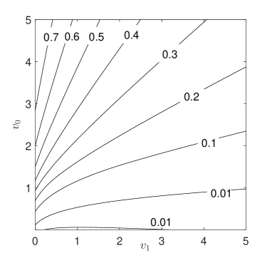
In the second experiment (Figure (b)), the costs $J_{\text{opt}}$ achieved by measuring at the optimal instant have been computed together with the costs $J_{\text{reg}}$ achieved by measuring at $\frac{T}{2}$. The values $T=1,\sigma^{2}=1$ and $v_{0},v_{1}$ varying from 00 to $5$ have been used for the parameters. Figure 3(b) shows a contour plot of the gain $\frac{J_{\text{reg}}-J_{\text{opt}}}{J_{\text{reg}}}$ as function of $v_{0},v_{1}$.

Figure 3(a) shows that measuring at the best instant among 00 and $\frac{T}{2}$ leads to a performance close to the optimal. Finding the correct ”regime“ is more important, therefore, than computing the optimal instant with high precision. The contour plot Figure 3(b) shows that for parameters $v_{0},v_{1}$ in the considered range, the gain can reach $81\%$.

$0.5$ $1$ $1.5$ $2$ $0.5$ $1$ $1.5$ $v_{0}$
$J_{T,v_{0},v_{1}}(0)$
$J_{T,v_{0},v_{1}}(\frac{T}{2})$
$J_{T,v_{0},v_{1}}(t^{(1)}_{\text{opt}})$
$\underline{J}(v_{0})$
Refer to caption
(a) (b)
Figure 3: (a) The costs for different choices of the instant of measurement $t_{1}$ compared with the lower bound $\underline{J}$ (see its definition (25)). The parameters equal: $T=1,\sigma^{2}=1,v_{1}=1$. (b) The contour plot of the gain of measuring at the optimal instant compared to measuring at $\frac{T}{2}$. The gain is defined as $\frac{J_{\text{reg}}-J_{\text{opt}}}{J_{\text{reg}}}$. The parameters equal: $T=1,\sigma^{2}=1,v_{0},v_{1}\in[0,5]$.

III-D Kalman filter with one Measure per Window, where the Windows are Periodic

If only one measure is possible during a finite time interval, the optimal instant for this measure has been determined. When a Brownian motion is observed over an infinite time, the following scheduling strategy can be established: measure at moments $t_{1,1}\in[0,T],t_{1,2}\in[T,2T],\dots,t_{1,k}\in[(k-1)T,kT],\dots$, where $t_{1,1}$ is chosen in order to minimize the mean variance over the interval $[0,T]$, then $t_{1,2}$ is chosen in order to minimize the mean variance over the interval $[T,2T]$ provided that the value $v(T)$ (which depends on $t_{1,1}$) is used as $v_{0}$ (i.e., $T$ is the left endpoint of the interval, and $v(T)$ is the variance of the prior information about $\theta(T)$), etc.

The parameters are: $T,v_{1}$ (the error variance of every measure) and $v_{0}$ (the variance of the prior information about $\theta(0)$). The intervals $[0,T],[T,2T],\dots$ will be called “windows”.

The main result of this section is Theorem 4: for $k$ big enough, $t_{1,k}=(k-1)T$, i.e. the measures are done at the left endpoints of the corresponding “windows”.

Theorem 4.

In the setting described above, the sequence of measurement instants satisfies: $t_{1,k}=(k-1)T$ for $k$ large enough. Therefore, it is ultimately periodic.

Theorem 4 is proved in Technical Report [2]. Figure 4 illustrates this setting:

$t$ $v$ $v_{0}=0.5$ $t_{1}$ $T$ $\frac{7}{6}$ $t_{1,1}$ $2T$ $1.5415$ $3T$ $1.7454$ $4T$ $1.8024$
Figure 4: $4$ iterations of the function $\mathcal{F}_{T,v_{1}}$ from the initial value $v_{0}=\frac{1}{2}$. The parameters are $v_{1}=1,\sigma^{2}=1,T=\frac{7}{6}$. The values $v_{0},v(T),v(2T),\dots$ are written on the figure.

One can remark that the result above resembles the results of [9]. In [9], the moments of measure are strictly periodic, while the sensor is chosen using a local optimization. On the other hand, in the present setting, the sensor cannot be chosen, while the instants of measure are chosen in periodic windows. Ultimate periodicity holds as a qualitative result in both cases.

IV The optimal instants of two measures.

IV-A Overview of the Results.

In this section, it is supposed that the observer is allowed to choose the instants $t_{1}$ and $t_{2}$ $(0\leqslant t_{1}\leqslant t_{2}\leqslant T)$ for $n{=}2$ measures with measurement noises $v_{1},v_{2}$ respectively. Certain questions listed in Section II-C above are answered with explicit formulas.

The cost function (12) can be expressed in one of the $3$ forms:

$$J_{\sigma^{2},T,v_{0},v_{1},v_{2}}(t_{1},t_{2})=\frac{\sigma^{2}t_{1}^{2}}{2}+v_{0}t_{1}+\frac{\sigma^{2}\triangle t_{2}^{2}}{2}+\\ \frac{(\sigma^{2}t_{1}+v_{0})v_{1}\triangle t_{2}}{\sigma^{2}t_{1}+v_{0}+v_{1}}+\frac{\sigma^{2}(T-t_{2})^{2}}{2}+\Gamma^{t_{2}}_{t_{2}}(T-t_{2})=\\ \frac{\sigma^{2}t_{1}^{2}}{2}+v_{0}t_{1}+J_{\sigma^{2},T-t_{1},\Gamma^{t_{1}}_{t_{1}},v_{2}}(t_{2}-t_{1})=\\ \frac{\sigma^{2}t_{1}^{2}}{2}{+}v_{0}t_{1}{+}\frac{\sigma^{2}\triangle t_{2}^{2}}{2}+\frac{(\sigma^{2}t_{1}{+}v_{0})v_{1}\triangle t_{2}}{\sigma^{2}t_{1}{+}v_{0}{+}v_{1}}+\frac{\sigma^{2}(T{-}t_{2})^{2}}{2}\\ +\frac{v_{2}(T-t_{2})\left(v_{1}(v_{0}+\sigma^{2}t_{1})+\sigma^{2}\triangle t_{2}(v_{1}+v_{0}+\sigma^{2}t_{1})\right)}{(v_{1}+v_{2})(v_{0}+\sigma^{2}t_{1})+v_{1}v_{2}+\sigma^{2}\triangle t_{2}(v_{1}+v_{0}+\sigma^{2}t_{1})},$$ (26)

where $\triangle t_{2}=t_{2}-t_{1}$.

It is proved (Theorems 5,6,7) that this cost function has a unique coordinatewize local minimum which is, therefore, a global minimum. A coordinatewize local minimum (CWLM) is defined, in an analogous way to [12] as follows.

Definition 1.

Let $f:D\subset\mathbb{R}^{2}\to\mathbb{R}$ be a real-valued function, and let $z=(z_{1},z_{2})\in D$. Then the point $z$ is called a coordinatewize local minimum (CWLM) of $f$ if

$\displaystyle\exists\epsilon>0$ $\displaystyle\ \forall d\in]-\epsilon,\epsilon[,$
$\displaystyle(z_{1}+d,z_{2})\in D$ $\displaystyle\implies f(z)+(d,0)\geqslant f(z)\text{ and}$
$\displaystyle(z_{1},z_{2}+d)\in D$ $\displaystyle\implies f(z)+(0,d)\geqslant f(z).$

The argmin of $J_{\sigma^{2},T,v_{0},v_{1},v_{2}}$ (unique) is denoted

$$(t^{(2)}_{1,\text{opt}}(\sigma^{2},T,v_{0},v_{1},v_{2}),t^{(2)}_{2,\text{opt}}(\sigma^{2},T,v_{0},v_{1},v_{2}))$$ (27)

in accordance with the general notation (13).

One of the general remarks is that, if $t_{1}$ is fixed, the subproblem of determining the optimal instant $t_{2}$ relative to $t_{1}$ is reduced to determining the optimal instant of one measure (see Section III) with the following parameters: the length of the process is $T-t_{1}$, the variance of the estimate of the initial state is $\Gamma^{t_{1}}_{t_{1}}$, the variance of the error of the measure is $v_{2}$.

$$\operatorname*{arg\,min}_{t_{2}}J_{\sigma^{2},T,v_{0},v_{1},v_{2}}(t_{1},t_{2})=t_{1}+t^{(1)}_{\text{opt}}(\sigma^{2},T-t_{1},\Gamma^{t_{1}}_{t_{1}},v_{2}).$$ (28)

Finding the minimum of the cost function $J_{\sigma^{2},T,v_{0},v_{1},v_{2}}$, studying its properties (uniqueness, position, etc) and its dependence on the parameters, such as monotonicity, continuity, is the goal of this section. An important property of the minimum is its position on the border or in the interior of the domain of definition of the function. It is sufficient to consider three qualitatively different properties of the optimal schedule (“regimes”): either $0=t_{1}=t_{2}$ (regime 1) or $0=t_{1}<t_{2}$ (regime 2) or $0<t_{1}\leqslant t_{2}$ (regime 3). Figure 5 shows examples of the cost function, which correspond to different regimes. This consideration is analogous to the one made in case of one measure.

Regime 1 is observed when $T$ is small enough. Then, if $t_{1}=0$ is fixed, the optimal instant for the second measure (determined by (28)) is also zero. By Theorem 5 below, this is equivalent to saying that $(0,0)$ is the globally optimal schedule of measures.

When regime 1 is not observed, the optimal instant for the second measure is strictly positive. One can search the optimal schedule using the coordinate descent from $(0,0)$. The first step is finding the optimal instant of the second measure when the first measure is done at 00 using (28). Call this instant $t_{2}^{\langle 1\rangle}\in]0,T]$. On the second step, find the optimal instant of the first measure, when the second measure is done at $t_{2}^{\langle 1\rangle}$. Call this instant $t_{1}^{\langle 1\rangle}\in[0,t_{2}^{\langle 1\rangle}[$. If $t_{1}^{\langle 1\rangle}=0$, the algorithm finishes and returns the schedule $(0,t_{2}^{\langle 1\rangle})$. This situation will be called regime 2. By Theorem 6, this schedule is indeed optimal.

Refer to caption
Refer to caption
Refer to caption
Figure 5: Examples of the cost function $J_{\sigma^{2},T,v_{0},v_{1},v_{2}}(t_{1},t_{2})$. In all plots, $\sigma^{2}=1$ and $v_{0}=v_{1}=v_{2}=1$. In the first example, $T=0.2$. In the second example, $T=0.5$. In the third example, $T=1.5$.
$0.2$ $0.4$ $0.95$ $1$ $1.05$ $t_{1}$ $J$ $0.5$ $1$ $1.5$ $2$ $5.8$ $6$ $6.2$ $6.4$ $6.6$ $t_{1}$ $J$ $0.5$ $1$ $1.5$ $2$ $8$ $9$ $10$ $11$ $t_{1}$ $J$
(a) (b) (c)
$0.5$ $1$ $1.5$ $2$ $7.2$ $7.4$ $7.6$ $t_{1}$ $J$ $0.5$ $1$ $1.5$ $2$ $5.8$ $6$ $6.2$ $6.4$ $t_{1}$ $J$ $0.5$ $1$ $1.5$ $2$ $3.6$ $3.8$ $4$ $t_{1}$ $J$
(d) (e) (f)
Figure 6: Examples of the cost function $t_{1}\mapsto J_{\sigma^{2},T,v_{0},v_{1},v_{2}}(t_{1},t_{2})$ in the examples of Figure 7. One can observe the difference between regime 2 (the function is increasing) and regime 3 (the minimum is located inside the interval).

In regime 3, the coordinate descent does not terminate after the first $2$ steps, i.e., $t_{1}^{\langle 1\rangle}>0$. Then it is optimal to perform both measures in the interior of the interval $[0,T]$ (Theorem 6). The distinction between regime 2 and regime 3 can be done by computing the partial derivative with respect to $t_{1}$ of the cost function (26) at $(0,t_{2}^{\langle 1\rangle})$ or, equivalently, by comparing $T$ to a critical value.

The largest duration $T$, such that regime 1 is observed, will be denoted $T^{(2)}_{2,\text{\rm crit}}$ (can be computed using (29)). Similarly, the largest duration $T$, such that regime 1 is observed, will be denoted $T^{(2)}_{1,\text{\rm crit}}$ (can be computed using (34)).

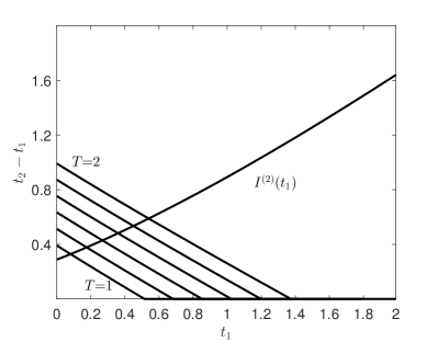
Figure 6 shows different examples of functions $t_{1}\mapsto J_{\sigma^{2},T,v_{0},v_{1},v_{2}}(t_{1},t_{2}^{\langle 1\rangle})$, which can be observed during the second step of this coordinate descent in sample situations.

Example $v_{0}$ $v_{1}$ $v_{2}$ $t_{2}^{<1>}$ $T$ $t_{1}^{<1>}$ Regime $T_{1,\text{crit}}$ $t^{(2)}_{1,\text{opt}}$ $t^{(2)}_{2,\text{opt}}$
a) $1$ $1$ $1$ $0.5$ $\frac{7}{6}$ 00 Critical $\frac{7}{6}$ 00 $0.5$
b) $1$ $1$ $1$ $2$ $\frac{71}{18}\approx 3.94$ $0.8668$ 3 $\frac{7}{6}$ $1.0401$ $2.4092$
c) $3$ $1$ $1$ $2$ $\frac{317}{76}\approx 4.17$ 00 2 $4.6500$ 00 $2$
d) $1$ $3$ $1$ $2$ $\frac{317}{76}\approx 4.17$ $0.9768$ 3 $1.1878$ $1.1211$ $2.985$
e) $1$ $1$ $3$ $2$ $\frac{123}{34}\approx 3.62$ $1.1044$ 3 $0.8630$ $1.1968$ $2.4269$
f) 00 $1$ $1$ $2$ $3.5$ $1.3538$ 3 00 $1.5107$ $2.4196$
Figure 7: Sample examples of the problem of seeking the optimal instants of two measurements. In all examples, it is supposed that $\sigma^{2}=1$ and the regime $1$ is not observed. The columns $v_{0},v_{1},v_{2},t_{2}^{<1>}$ are parameters, while the other columns can be computed using the formulae of the present article. Figure 6 shows the functions to optimize when finding $t_{1}^{<1>}$ during the first step of the coordinate descent.

Section IV is organized as follows.

A criterion of regime 1 together with a proof that the optimal schedule does not satisfy $0<t^{(2)}_{\text{opt}}=t^{(2)}_{2,\text{opt}}$ (Lemma 1) is given in Subsection IV-C. The critical regime, on the border between regimes $2$ and $3$, is studied in Subsection IV-D. In particular, formulas in closed form are found for finding, to which regime belongs a given set of parameters $\sigma^{2},T,v_{0},v_{1},v_{2}$.

Equations for the optimal instants in regime $3$ follow from the results of Subsection IV-D. These are discussed in Section IV-E. Some properties of the optimal instants are deduced from these equations.

The coordinate descent algorithm can be used for finding the optimal measurement instants in regime 3. It is shown that this algorithm cannot converge to a point different from the global minimum of the cost function. This follows from the uniqueness of a CWLM of the cost function $J(t_{1},t_{2})$ (Theorem 9, Section IV-E).

IV-B Strategy of proof.

Proving the uniqueness of a CWLM of the cost function $J(t_{1},t_{2})$ is done by considering first the borders of its domain of definition, then the interior. The border $t_{1}=t_{2}$ (represented by the diagonal in the plots Figure 5) is studied in Subsection IV-C. The border $t_{1}=0$ (represented by the left side in the plots Figure 5) is studied in Subsection IV-D. The schedules on the border $t_{2}=T$ can be improved upon by decreasing $t_{2}$ according to the results relative to one measure. The interior is studied in Subsections IV-D and IV-E using the previous results.

IV-C Simultaneous measurements ($t_{1}=t_{2}$).

Taking both measures at the same time makes them equivalent to a single measure of smaller error variance $v_{1,2}$. Therefore, the performance of such schedule is the same as one achieved by one measure. Lemma 1 shows that, except the case where the measures are at the instant 00, such schedule can be improved upon by a small displacement of the instant of one measure. The rest of this subsection is devoted to studying the optimality of taking both measures at 00 (regime 1).

Lemma 1.

Consider the cost function (26) defined on the triangular domain ${\mathcal{T}}_{T}=\{(t_{1},t_{2})\text{ s.t.}0\leqslant t_{1}\leqslant t_{2}\leqslant T\}$. Let $0<t_{1}<T$. Then the point $(t_{1},t_{1})$ is not a coordintewize local minimum of $J_{\sigma^{2},T,v_{0},v_{1},v_{2}}(t_{1},t_{2})$.

Lemma 1 is proved in Technical Report [2]. It corresponds to the intuitive idea that the instants of measure have a tendency to “repulse” each other.

The following criterion for deciding whether both optimal instants equal zero (regime 1) extends the criterion (17) from the case of one measure to the case of two measures.

Theorem 5.

The global minimum of the cost function (26) is reached at the point $(0,0)$ if and only if

$$T\leqslant T^{(2)}_{2,\text{\rm crit}}(\sigma^{2},v_{0},v_{1},v_{2})=T^{(1)}_{\text{\rm crit}}(\sigma^{2},v_{0,1},v_{2})=\\ \frac{v_{0,1}}{\sigma^{2}\left(\frac{v_{2}}{v_{0,1}+v_{2}}+1\right)}.$$ (29)

Moreover, when (29) holds, the point $(0,0)$ is the unique CWLM of the function (26).

Proof.

Direct part. Suppose the minimum is at $(0,0)$. In particular, the function

$$t_{2}\mapsto J_{\sigma^{2},T,v_{0},v_{1},v_{2}}(0,t_{2})=J_{\sigma^{2},T,v_{0,1},v_{2}}(t_{2})$$ (30)

has its minimum at $t_{2}=0$, therefore the regime 1 in the sense of a single measure is observed (cf Subsection III-B). Therefore, the criterion (17) applied to the parameters $\sigma^{2},T,v_{0,1},v_{2}$ is valid. This is (29).

Inverse part. Suppose $T\leqslant T^{(2)}_{2,\text{crit}}$. For any $t_{1}\in[0,T[$ the minimum of the function

$$[t_{1},T]\ni t_{2}\mapsto J_{\sigma^{2},T,v_{0},v_{1},v_{2}}(t_{1},t_{2})=\\ \frac{\sigma^{2}t_{1}^{2}}{2}+v_{0}t_{1}+J_{\sigma^{2},T-t_{1},\Gamma^{t_{1}}_{t_{1}},v_{2}}(t_{2}-t_{1})$$ (31)

is the same as the minimum of

$$[t_{1},T]\ni t_{2}\mapsto J_{\sigma^{2},T-t_{1},\Gamma^{t_{1}}_{t_{1}},v_{2}}(t_{2}-t_{1})$$ (32)

and can be found using the results of Subsection III-B. More precisely, regime $1$ is observed. Indeed, as the function $v_{0}\mapsto T^{(1)}_{\text{crit}}(\sigma^{2},v_{0},v1)$ is increasing and $\Gamma^{t_{1}}_{t_{1}}\geqslant v_{0,1}$, one has

$$T-t_{1}\leqslant T\leqslant T^{(1)}_{\text{crit}}(\sigma^{2},v_{0,1},v_{2})\leqslant T^{(1)}_{\text{crit}}(\sigma^{2},\Gamma^{t_{1}}_{t_{1}},v_{2}).$$ (33)

This implies that, under the hypothesis $T\leqslant T^{(2)}_{2,\text{crit}}$, all CWLM’s of the cost function $J_{\sigma^{2},T,v_{0},v_{1},v_{2}}(t_{1},t_{2})$ are points of the type $(t_{1},t_{1})$, that is, on the diagonal. By Lemma 1, the only candidate for being a CWLM of $J_{\sigma^{2},T,v_{0},v_{1},v_{2}}(t_{1},t_{2})$ is the point $(0,0)$, which is, therefore, its global minimum.

Remark that the critical duration $T^{(2)}_{2,\text{crit}}$ is an increasing function of $v_{0}$ and of $v_{1}$, a decreasing function of $\sigma^{2}$ and of $v_{2}$.

It is proved in this subsection that a CWLM on the diagonal can only be achieved at $(0,0)$. Moreover, (29) provides a necessary and sufficient condition (depending on the parameters), which allows one to check whether $(0,0)$ is indeed a CWLM. This is equivalent to regime 1.

IV-D The boundary $t_{1}=0$.

If (29) does not hold, consider the boundary $t_{1}{=}0$. Taking the first measure at zero leads to the same performance as the setting with one measure of error variance $v_{2}$ and initial information of smaller error variance $v_{0,1}$. Theorem 6 shows that the optimal schedule is of this type for some values of parameters. This subsection is devoted to studying when this is satisfied.

The following result answers the question, whether the minimum is located on the boundary.

Theorem 6.

The global minimum of the cost function $J_{\sigma^{2},T,v_{0},v_{1},v_{2}}$ is located on the line $(0,\cdot)$ iff $T\leqslant T^{(2)}_{1,\text{\rm crit}}(\sigma^{2},v_{0},v_{1},v_{2})$, where

$$T^{(2)}_{1,\text{\rm crit}}(\sigma^{2},v_{0},v_{1},v_{2})=T_{t_{1}}(\sigma^{2},t_{2,1,\text{\rm crit}}(\sigma^{2},v_{0},v_{1},v_{2}),v_{0,1},v_{2}).$$ (34)

Here, the function $T_{t_{1}}$ is defined by

$$T_{t_{1}}(\sigma^{2},t_{1},v_{0},v_{1})=2t_{1}+\frac{v_{0}-v_{1}}{\sigma^{2}}+\frac{2v_{1}^{2}}{\sigma^{2}(v_{0}+\sigma^{2}t_{1}+2v_{1})}$$ (35)

and $\sigma^{2}t_{2,1,\text{\rm crit}}(\sigma^{2},v_{0},v_{1},v_{2})$ is the largest root of the equation

$$Ax^{3}+Bx^{2}+Cx+D=0$$ (36)

with coefficients

$\displaystyle A(v_{0},v_{1},v_{2})$ $\displaystyle=-(v_{0}+v_{1})^{2}(v_{0}+2v_{1}),$ (37)
$\displaystyle B(v_{0},v_{1},v_{2})$ $\displaystyle=(v_{0}+v_{1})\times$
$\displaystyle(v_{0}^{3}-3((v_{0}+v_{1})(v_{0}+2v_{1})v_{2}+v_{0}v_{1}^{2})),$ (38)
$\displaystyle C(v_{0},v_{1},v_{2})$ $\displaystyle=v_{2}B(v_{0},v_{1},v_{2})+$
$\displaystyle v_{0}^{2}(2v_{0}+3v_{1})(v_{0}v_{1}+v_{0}v_{2}+v_{1}v_{2}),$ (39)
$\displaystyle D(v_{0},v_{1},v_{2})$ $\displaystyle=v_{0}^{2}(v_{1}+v_{2})(v_{0}+v_{1})\times$
$\displaystyle(v_{0}v_{1}+2v_{0}v_{2}+3v_{1}v_{2}).$ (40)

If $T\leqslant T^{(2)}_{1,\text{crit}}(\sigma^{2},v_{0},v_{1},v_{2})$, the minimum of the cost function is located at the point $(0,t_{2}^{\langle 1\rangle})$, where

$$t_{2}^{\langle 1\rangle}=t^{(1)}_{\text{\rm opt}}(\sigma^{2},T,v_{0,1},v_{2})$$ (41)

according to the more general equation (28).

Theorem 6 is proved in the Technical Report [2].

According to Theorems 6 and 5, the optimal schedule is of the form $(0,\cdot)$, but not $(0,0)$ if and only if

$$T^{(2)}_{2,\text{\rm crit}}(\sigma^{2},v_{0},v_{1},v_{2})<T\leqslant T^{(2)}_{1,\text{\rm crit}}(\sigma^{2},v_{0},v_{1},v_{2}),$$ (42)

where $T^{(2)}_{1,\text{\rm crit}}$ is defined by (34)-(40) and $T^{(2)}_{2,\text{\rm crit}}$ is defined by (29). This case will be called regime 2.

The proof of Theorem 6 immediately leads to the following corollaries.

Corollary 1.

If $T\leqslant T^{(2)}_{1,\text{\rm crit}}(\sigma^{2},v_{0},v_{1},v_{2})$, the point $(0,t_{2}^{\langle 1\rangle})$ is the only CWLM of the cost function.

Corollary 2.

Let $\sigma^{2},v_{1},v_{2}\in\mathbb{R}_{+}^{*}$. Then, the critical durations $T^{(2)}_{1,\text{\rm crit}},T^{(2)}_{2,\text{\rm crit}}$ as well as the duration $t_{2,1,\text{\rm crit}}$, appearing in the formulation of Theorem 6, are strictly increasing functions of $v_{0}$.

The quantity $t_{2,1,\text{\rm crit}}$, appearing in the formulation of Theorem 6 has the following interpretation: the optimal schedule in the case of the duration $T=T^{(2)}_{1,\text{crit}}(\sigma^{2},v_{0},v_{1},v_{2})$ is $(0,t_{2,1,\text{\rm crit}})$.

IV-E The general case and its Properties.

Suppose that the process is long enough, i.e. $T>T^{(2)}_{1,\text{crit}}(\sigma^{2},v_{0},v_{1},v_{2})$. Therefore, regime 3 is observed (Theorem 6). In this subsection, equations for determining the optimal instants of measure $t^{(2)}_{1,\text{opt}}$ and $t^{(2)}_{2,\text{opt}}$ will be derived. Nontrivial optimal instants, which cannot be computed using formulae for $1$ measure, are defined in this section, and some properties of these optimal instants are proved.

Theorem 7.

Suppose that the length of the process is larger than the critical durations: $T>T^{(2)}_{1,\text{\rm crit}}(\sigma^{2},v_{0},v_{1},v_{2})$. Then, the cost function $J_{\sigma^{2},T,v_{0},v_{1},v_{2}}$ has a unique CWLM $(t^{(2)}_{1,\text{\rm opt}},t^{(2)}_{2,\text{\rm opt}})$, and it satisfies

$\displaystyle t^{(2)}_{2,\text{\rm opt}}-t^{(2)}_{1,\text{\rm opt}}$ $\displaystyle=t_{\text{\rm opt}}^{(1)}(\sigma^{2},T-t_{1,\text{\rm opt}}^{(2)},(v_{0}+\sigma^{2}t_{1,\text{\rm opt}}^{(2)})\mathbin{\!/\mkern-5.0mu/\!}v_{1},v_{2}),$ (43)
$\displaystyle t^{(2)}_{2,\text{\rm opt}}-t^{(2)}_{1,\text{\rm opt}}$ $\displaystyle=t_{2,1,\text{\rm crit}}(\sigma^{2},v_{0}+t^{(2)}_{1,\text{\rm opt}},v_{1},v_{2}),$ (44)

where the function $t_{2,1,\text{\rm crit}}$ is defined as the largest real root of the equation (36) with coefficients (37)-(40), and the function $t_{\text{\rm opt}}^{(1)}$ is defined Equation (15). Moreover, the system of equations (43),(44) has a unique solution with respect to the variables $t^{(2)}_{1,\text{\rm opt}},t^{(2)}_{2,\text{\rm opt}}-t^{(2)}_{1,\text{\rm opt}}\in\mathbb{R}_{+}^{*}$.

Theorem 7 is proved in Technical Report [2].

The system of equations (43),(44) is of the form

$$\left\{\begin{aligned} y&=I^{(1)}_{\sigma^{2},T,v_{0},v_{1},v_{2}}(x)\\ y&=I^{(2)}_{\sigma^{2},v_{0},v_{1},v_{2}}(x)\end{aligned}\right.$$

where $x=t^{(2)}_{1,\text{\rm opt}}$ and $y=t^{(2)}_{2,\text{\rm opt}}-t^{(2)}_{1,\text{\rm opt}}$. It is interesting to study the behavior of the functions $I^{(1)}$ and $I^{(2)}$, which appear in this system. Their full definitions are

$$I^{(1)}_{\sigma^{2},T,v_{0},v_{1},v_{2}}(\tilde{t}_{1})=\left\{\begin{array}[]{l}0\text{ if $\tilde{t}_{1}\geqslant T$}\\ t_{\text{opt}}^{(1)}(\sigma^{2},T-\tilde{t}_{1},(v_{0}+\sigma^{2}\tilde{t}_{1})\mathbin{\!/\mkern-5.0mu/\!}v_{1},v_{2})\\ \text{ otherwize.}\end{array}\right.$$ (45)

and

$$I^{(2)}_{\sigma^{2},v_{0},v_{1},v_{2}}(\tilde{t}_{1})=t_{2,1,\text{\rm crit}}(\sigma^{2},v_{0}+\sigma^{2}\tilde{t}_{1},v_{1},v_{2}).$$ (46)

Here, the continuation of the function $I^{(1)}(\tilde{t}_{1})$ by zero for large values serves a purely technical purpose.

The function $I^{(2)}$ has the following interpretation. Given the parameters $\sigma^{2},v_{0},v_{1},v_{2}$, to each $\tilde{t}_{1}\in\mathbb{R}_{+}$, a unique duration $T$ is associated such that $\tilde{t}_{1}$ is the optimal instant of the first measure. Then, $I^{(2)}(t_{1})$ is the distance between the optimal instants for the duration $T$. By Corollary 2, it is strictly increasing.

The function $I^{(1)}$ has a simpler definition and its interpretation is: given $\sigma^{2},T,v_{0},v_{1},v_{2}$, it associates to each $\tilde{t}_{1}$ (suboptimal in general) the best interval $\tilde{t}_{2}-\tilde{t}_{1}$ between the measures. The function $I^{(1)}$ “selects” the point associated to the given length $T$ on the graph of $I^{(2)}_{\sigma^{2},v_{0},v_{1},v_{2}}$. It is decreasing by Proposition 2. The optimal schedule corresponds to the intersection point of the graphs of these functions.

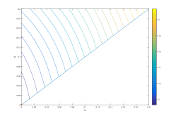
Figure 8 shows an example of the behavior of the functions $I^{(1)}$ and $I^{(2)}$.

Refer to caption
Figure 8: The functions $I^{(2)}(t_{1})$ and $I^{(1)}_{T}(t_{1})$. The fixed parameters are $\sigma^{2}=1,v_{0}=1,v_{1}=2,v_{3}=3$. $T$ takes values $1,1.2,1.4,1.6,1.8,2$. The optimal instant of first measure $t^{(2)}_{1,\text{\rm opt}}$ is the abscissa of the point of intersection. The distance between the measures in the optimal schedule is the ordinate of the point of intersection.

The next theorems assemble results for all three regimes and answer to conjectures announced in Sections II-C and IV-A.

Theorem 8.

Let $\sigma^{2},v_{0},v_{1},v_{2}\in\mathbb{R}_{+}^{*}$. For each $T\geqslant 0$, the minimizer of the cost function $J_{\sigma^{2},T,v_{0},v_{1},v_{2}}$ is unique.

The functions $T\mapsto t^{(2)}_{1,\text{\rm opt}}(\sigma^{2},T,v_{0},v_{1},v_{2})$ and $T\mapsto t^{(2)}_{2,\text{\rm opt}}(\sigma^{2},T,v_{0},v_{1},v_{2})$ are continuous and monotonically increasing.

Theorem 8 is proved in the Technical Report [2].

Moreover, the cost functions $J(t_{1},t_{2})$ have unique CWLM’s.

Theorem 9.

Let $\sigma^{2},v_{0},v_{1},v_{2},T\in\mathbb{R}_{+}^{*}$. Then, the function $J_{\sigma^{2},T,v_{0},v_{1},v_{2}}(t_{1},t_{2})$ has a unique CWLM.

Proof.

The theorem follows from Theorem 5 (in case of regime 1), Theorem 6 (in case of regime 2) and Theorem 7 (in case of regime 3). ∎

The global behavior of the optimal instants is illustrated Figure 9. Both measures should be done as fast as possible for small $T$ (regime 1). When the duration $T$ is larger than a critical value $T^{(2)}_{2,\text{crit}}$, the instant of the second measure becomes distinct from zero and increases (regime 2). When the duration $T$ is larger than another critical value $T^{(2)}_{1,\text{crit}}$, the instant of the first measure becomes distinct from zero as well and increases (regime 3). Both optimal instants of measure exhibit continuity at the critical durations. This behavior is in accordance with Theorems 5, 6 and 8.

$0.5$ $1$ $1.5$ $2$ $2.5$ $3$ $0.5$ $1$ $1.5$ $2$ $t_{1,\text{opt}}(T)$ $t_{2,\text{opt}}(T)$ $T^{(2)}_{2,\text{crit}}$mm$T^{(2)}_{1,\text{crit}}$ $t_{2,1,\text{crit}}$ $T$
$t_{2,\text{opt}}(T)$
$t_{1,\text{opt}}(T)$
Figure 9: $t^{(2)}_{1,\text{\rm opt}}(\sigma^{2},T,v_{0},v_{1},v_{2})$ and $t^{(2)}_{2,\text{\rm opt}}(\sigma^{2},T,v_{0},v_{1},v_{2})$ as functions of $T$ in a particular case. The parameters are $\sigma^{2}=1,v_{0}=v_{1}=v_{2}=1,T\in]0,5]$. In this example, the critical durations equal: $T^{(2)}_{2,\text{crit}}=0.3$ and $T^{(2)}_{1,\text{crit}}=\frac{7}{6}$. For $T=\frac{7}{6}$, the optimal schedule is $(0,0.5)$.

IV-F The numerical algorithm of Coordinate Descent.

Theorem 7 provides a convenient theoretical description of the optimal schedule $(t^{(2)}_{1,\text{\rm opt}},t^{(2)}_{2,\text{\rm opt}})$ in regime 3. Let us look for an efficient algorithm for finding numeric values of these instants. The coordinate descent is proposed as such algorithm in this article. The first step of the coordinate descent is important as well in defining the $3$ regimes. This algorithm is described in Appendix V.

Updating $t_{1}$ is finding the minimum of a cost function $J(t_{1})$ of a special type defined on a real interval. The golden-section search is used in this step. Some examples of functions this class are given Figure 6. It can be conjectured that all functions of this class are quasi-convex. If the function $J(t_{1})$ is quasi-convex, the golden-section search is guaranteed to converge to the minimum of this function.

The cost function $J(t_{1},t_{2})$ is guaranteed to have only one CWLM, therefore the coordinate descent cannot converge to a point different from the global minimum of the function.

IV-G The Experimental Performance of the Coordinate Descent.

100100100 
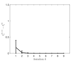
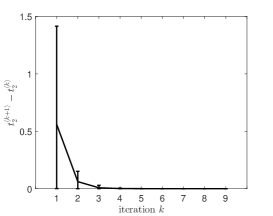
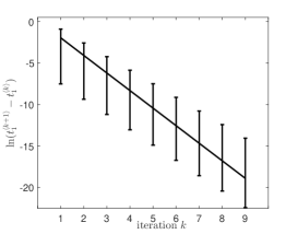
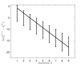
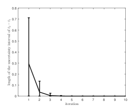
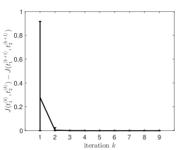
random runs of the algorithm have been performed in order to explore its convergence and the speed of convergence.

The parameters $\sigma^{2}=1$ and $T=10$ were fixed and the triples $(v_{0},v_{1},v_{2})$ were chosen randomly from the region of the cube $[1,10]^{3}$, which corresponds to regime 3, according to the uniform distribution. More precisely, candidate points were chosen in $[1,10]^{3}$, then they were use in the experiment if they satisfied the condition of regime 3: $T^{(2)}_{1,\text{crit}}(\sigma^{2},v_{0},v_{1},v_{2})>T$.

The results are shown Figure 10. They suggest an exponential convergence. Furthermore, the steps became shorter than $2\cdot 10^{-6}$ after less than $10$ steps in all runs.

Refer to caption Refer to caption Refer to caption
(a) (b) (c)
Refer to caption Refer to caption Refer to caption
(d) (e) (f)
Figure 10: Test performances of coordinate descent. The fixed parameters are $\sigma^{2}=1,T=10.$ $v_{0},v_{1},v_{2}$ have been drawn uniformly w.r.t. the Lebesgue measure from the part of the cube $[1,10]^{3}$ which corresponds to regime 3. (a) The increments of $t_{1}$. (b) The increments of $t_{2}$. (c) The natural logarithms of the increments of $t_{1}$. (d) The natural logarithms of the increments of $t_{2}$. (e) The difference $I^{(1)}_{\sigma^{2},T,v_{0},v_{1},v_{2}}(t_{1})-I^{(2)}_{\sigma^{2},v_{0},v_{1},v_{2}}(t_{1})$. According to Theorem 7, the values of the functions $I^{(1)},I^{(2)}$ are estimations of the difference $t^{(2)}_{2,\text{\rm opt}}-t^{(2)}_{1,\text{\rm opt}}$ and they are equal only for the optimal value of $t_{1}$. (f) The decrements of the cost function $J$. The abscissa of every graph is the number of the step. The lines join the mean values of the corresponding quantities over all trials. The vertical error bars show the maxima and the minima.

IV-H Comparison between the optimal and the regular schedules.

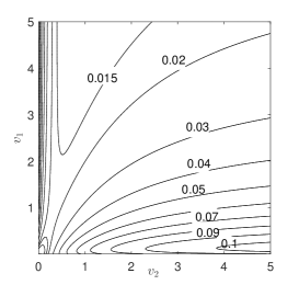
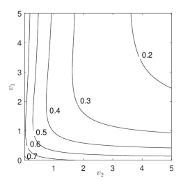
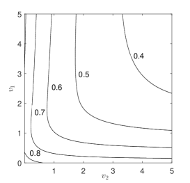
A numerical experiment of estimation of the gain of the optimal schedule compared to the intuitive sampling $(\frac{T}{3},\frac{2T}{3})$ has been done. The optimal schedules $(t^{(2)}_{1,\text{opt}},t^{(2)}_{2,\text{opt}})$ have been computed together with the associated costs $J_{\text{opt}}$ for $\sigma^{2}=1,T=1,v_{0}\in\{0,2,5\}$ and $v_{1},v_{2}$ varying from 00 to $5$. The costs $J_{\text{reg}}$ achieved with the regular sampling have been computed as well. Figure 11 shows three contour plots of the gain $\frac{J_{\text{reg}}-J_{\text{opt}}}{J_{\text{reg}}}$ as functions of $v_{1},v_{2}$.

Refer to caption Refer to caption Refer to caption
(a) (b) (c)
Figure 11: The relative gain achieved by the optimal schedule as functions of $v_{1},v_{2}\in[0,5]$. (a) $v_{0}=0$. The contours correspond to the values $0.01,0.015$, and $0.02$ to $0.1$ by steps of $0.01$. (b) $v_{0}=2$. (c) $v_{0}=5$.

These figures can be compared with the gain in case of $1$ measure (Figure 3). For parameters in the considered range, the gain can reach up to $86\%$.

V Conclusion and Perspectives

Sampling strategies for a phenomenon of finite length have been investigated under the assumption that the phenomenon can only be measured a small number of times by instruments with different properties (error variances). Irregular sampling can lead to a substantial gain in mean error variance of the estimator.

The assumption of a small number of available measures can be satisfied if the process itself is short or the measurement devices have a limited (and non-renewable) physical resource, e. g., [11]. This can also happen if each measure is expensive.

A simple model is studied, where the variance about the system parameters (here a single parameter) evolving over a finite period of time grows linearly in the absence of measure. The properties of the optimal measure timetable according to the criterion of minimization of the mean variance are considered.

In Section III, the particular case, where the instant of exactly $1$ measure is to be chosen, is studied in detail. Section IV is devoted to the particular case, where the instants of $2$ measures are to be chosen.

The system can behave in different regimes. When the duration of the process is short, it is optimal to take all measures at the moment zero. If it is larger, than a critical value, one optimal instant of measure moves from zero to the inside of the interval. In the case of one measure, there is one critical duration, while in case of two measures there are two.

It is proved that the critical durations in case of 1 or 2 measures are increasing functions of $v_{0}$. This corresponds to a simple intuition: the larger $v_{0}$ is, the less exact is the information, the higher are chances that it should be supported by a measure. This corresponds to the intuition stated in the introduction: in the optimal sampling, the more precise measure may be made shortly after the less precise one.

The computations relative to the case $n=2$ (shown Figure 11) suggest that when $v_{0}\ll\sigma^{2}T,v_{1},v_{2}$, the gain in comparison with the regular schedule is modest. On the other hand, it increases if the variance $v_{0}$ of the initial information increases or if the variances $v_{1},v_{2}$ of the measures are very different. The first conclusion is also confirmed experimentally in case of $1$ measure (see Figure 3 (b)).

A setting, where a large number of measures are made under a constraint of periodic “windows”, is considered Section III-D. The instants of measurement are determined using local optimization. It is shown that local optimization leads to regular sampling (Theorem 4) when the number of measures is large. This result suggests that the global optimization is necessary for getting an improvement of performance.

One goal of the future research is to find the optimal (in the sense of the cost function (12)) measurement instants when the number of measures is $n>2$. The methods of this article can be adapted. Some qualitatively new conjectures also appear from the experiments in this setting. Allowing the number of measures to vary is another possible development of the results presented here.

In this problem, the order of the measures is fixed. It is also possible to allow it to vary. The main property of this problem is the fact that the cost function is no longer rational, but piecewise-rational.

Another objective of the future research is to consider more complex models than the real Brownian motion considered presently.

[Pseudo-code of the coordinate descent algorithm.]

1:  if $T\leqslant\frac{v_{0,1}}{\sigma^{2}\left(\frac{v_{2}}{v_{0,1}+v_{2}}+1\right)}$ then
2:     return  $(0,0)$ (regime 1)
3:  else
4:     $t_{2}^{\langle 1\rangle}:=t_{\text{opt}}^{(1)}(\sigma^{2},T,v_{0,1},v_{2})$
5:     if $A(v_{0},v_{1},v_{2})(\sigma^{2}t_{2}^{\langle 1\rangle})^{3}+B(v_{0},v_{1},v_{2})(\sigma^{2}t_{2}^{\langle 1\rangle})^{2}+C(v_{0},v_{1},v_{2})\sigma^{2}t_{2}^{\langle 1\rangle}+D(v_{0},v_{1},v_{2})\geqslant 0$ then
6:        return  $(0,t_{2}^{\langle 1\rangle})$ (regime 2)
7:     else
8:        Initialization (regime 3, coordinate descent)
9:        $t_{2}:=t_{2}^{\langle 1\rangle}$
10:        $t_{1}:=t_{1}^{\langle 1\rangle}=\operatorname*{arg\,min}_{t_{1}}J_{\sigma^{2},T,v_{0},v_{1},v_{2}}(t_{1},t_{2}^{\langle 1\rangle})$
11:        repeat
12:           $t_{2}:=t_{2}^{\langle k\rangle}=t_{1}^{\langle k-1\rangle}+t_{\text{opt}}^{(1)}(\sigma^{2},T-t_{1}^{\langle k-1\rangle},(v_{0}+\sigma^{2}t_{1}^{\langle k-1\rangle})\mathbin{\!/\mkern-5.0mu/\!}v_{1},v_{2})$
13:           $t_{1}:=t_{1}^{\langle k\rangle}=\operatorname*{arg\,min}_{t_{1}}J_{\sigma^{2},T,v_{0},v_{1},v_{2}}(t_{1},t_{2}^{\langle k\rangle})$
14:        until convergence
15:     end if
16:  end if
Figure 12: Compute the optimal instants of $2$ measures. Arguments: $\sigma^{2},T,v_{0},v_{1},v_{2}\in\mathbb{R}_{+}^{*}$.

References

  • [1] A. Aksenov, P.-O. Amblard, O. Michel, Ch. Jutten, “Optimal measuremet times for observing a Brownian motion over a finite period using a Kalman filter” (2016), Lecture Notes in Computer Science, Volume 10169.
  • [2] A. Aksenov, P.-O. Amblard, O. Michel, Ch. Jutten, “Technical report for the article “Optimal Measurement Times for a Small Number of Measures of a Brownian Motion over a Finite Period”.
  • [3] A.Bourrier, P.-O. Amblard, O.Michel, Ch.Jutten. “Multimodal Kalman filtering” IEEE International Conference on Acoustics, Speech and Signal Processing (ICASSP), Mar 2016, Shanghai, China.
  • [4] Vijay Gupta, Timothy H. Chung, Babak Hassibi, Richard M. Murray “On a Stochastic Sensor Selection Algorithm in Sensor Scheduling and Sensor Coverage” textitAutomatica, Vol. 42, Issue 2 (Feb 2006), 251–260.
  • [5] David L.Hall, James Linas “An Introduction to Multisensor Data Fusion” textitProceedings of the IEEE, Vol. 85, No. 1 (Jan 1997), 6–38.
  • [6] K. Herring, J. Melsa, “Optimum measurements for estimation” IEEE Transactions on Automatic Control, Vol. 19, Issue 3 (1974), 264–266.
  • [7] Andrew H. Jazwinski, Stochastic processes and filtering theory, Mathematics in science and engineering. Academic Press, New York, 1970, UKM
  • [8] D.Lahat, T.Adalı, Ch.Jutten “Multimodal Data Fusion: An Overview of Methods, Challenges and Prospects” Proccedings of the IEEE, Vol. 103, Issue 9 (Sept 2015), 1449–1477.
  • [9] L.Orihuela, A.Barreiro, F.Gómez-Estern, F.R.Rubio “Periodicity of Kalman-based scheduled filters” Automatica 50 (2014), 2672-2676.
  • [10] Stergios I. Roumeliotis, George A. Bekey “Distributed Multi-Robot Localization” Distributed Autonomous Robotic Systems 4, 179–188.
  • [11] P.G. Ryan, S.L. Petersen, G. Peters, D. Grémillet “GPS tracking a marine predator: the effects of precision, resolution and sampling rate on forading tracks of African Penguins.” Marine Biology 145 (2004), 215-223.
  • [12] P.Tseng “Convergence of a Block Coordinate Descent Method for Nondifferentiable Minimization.” Journal of Optimization Theory and Applications 109 No.3 (June 2001), 475–494.
  • [13] Andrew Warrington and Neil Dhir “Generalising Cost-Optimal Particle Filtering” ICRA 2018: Workshop on Informative Path Planning and Adaptive Sampling (May 2018)