Combinatorial and Algorithmic Properties of One Matrix Structure at Monotone Boolean Functions

Abstract

One matrix structure in the area of monotone Boolean functions is defined here. Some of its combinatorial, algebraic and algorithmic properties are derived. On the base of these properties three algorithms are built. First of them generates all monotone Boolean functions of $n$ variables in lexicographic order. The second one determines the first (resp. the last) lexicographically minimal true (resp. maximal false) vector of an unknown monotone function $f$ of $n$ variables. The algorithm uses at most $n$ membership queries and its running time is $\Theta(n)$. It serves the third algorithm, which identifies an unknown monotone Boolean function $f$ of $n$ variables by using membership queries only. The experimental results show that for $1\leq n\leq 6$, the algorithm determines $f$ by using at most $m.n$ queries, where $m$ is the combined size of the sets of minimal true and maximal false vectors of $f$.

Keywords: monotone Boolean function; matrix structure properties; generating algorithm; minimal true vector; maximal false vector; identification algorithm
Note (Feb. 15, 2019). This manuscript was written in 2005 and has not been published till now. This is its original version where few misprints have been corrected and the Internet references have been updated.

1 Introduction

The problems in the area of monotone Boolean functions (MBFs) are important not only for the Boolean algebra. Many of them are related to (or they have a direct interpretation in) problems, arising in various fields, such as graph (hypergraph) theory, threshold logic, circuit theory, artificial intelligence, computation learning theory, game theory etc. [2, 6, 15]. Some problems, concerning MBFs, are still not solved in the general case, others have still open complexities. Some well-known scientists consider that the capabilities of the known tools and methods for investigation of MBFs are still not efficient enough and they recommend new approaches and tools to be searched and used [5, 15]. This opinion additionally motivated us to do the following investigations and to represent them here.

Three of the well known problems, concerning MBFs are:

(1) The Dedekind’s problem – for enumeration of the MBFs of $n$ variables (or, equivalently, for enumeration of all antichains of subsets of an $n$-set). The problem is set by Dedekind in the end of 19th century, it is the oldest problem in the area of MBFs [20];

(2) The identification problem – for identification of an unknown MBF of $n$ variables by using a given learning model;

(3) Determining at least one minimal true vector and/or at least one maximal false vector of an unknown MBF. This problem is closely related to the problem (2).

Here we represent our investigations of these three problems. Firstly, in Section 2, we recall some necessary notions and known results. In Section 3 we define one matrix structure, which represents the precedences of the vectors of the $n$-dimensional Boolean cube. Some combinatorial and algorithmic properties of the structure are derived. On the base of them we build three algorithms. The first of them is represented in Section 4. It generates all MBFs of $n$ variables in lexicographic order and it works in polynomial total time. The second one has two versions and it is described in Section 5. It determines the first (resp. the last) lexicographically minimal true (resp. maximal false) vector of an unknown MBF of $n$ variables. The algorithm is of the type binary search, it has $\Theta(n)$ running time and uses at most $n$ membership queries for each of these vectors. Section 6 represents the third algorithm which identifies an unknown MBF of $n$ variables by using membership queries only. It uses the second algorithm and obeys to the ”Divide and conquer” strategy. Some comments concerning the realizations, the complexity and the experimental results of the algorithm are also given.

2 Basic notions and preliminary results

One of the famous notions in Discrete mathematics is the $n$-dimensional Boolean cube $\{0,1\}^{n}$ – the $n$-th Cartesian power of the set $\{0,1\}$, consisting of all $n$-dimensional binary vectors, i.e., $\{0,1\}^{n}$$\ =\{\mbox{$({a}_{1},{a}_{2},\dots,{a}_{n})$}|\,a_{i}\in\{0,1\},\ i=1,2,\dots,n\}$. Obviously, these vectors are exactly $2^{n}$. The serial number of the vector $\alpha=(a_{1},a_{2}$, $\dots,a_{n})\in\mbox{$\{0,1\}^{n}$}$ is the natural number $\#\alpha=a_{1}.2^{n-1}+a_{2}.2^{n-2}+\dots+a_{n}.2^{0}$, i.e., the natural number whose binary representation is $a_{1}a_{2}\dots a_{n}$. The vector $\alpha\in\mbox{$\{0,1\}^{n}$}$ precedes lexicographically the vector $\beta\in\mbox{$\{0,1\}^{n}$}$ if either there exists an integer $k,1\leq k\leq n$, such that $a_{k}<b_{k}$ and $a_{i}=b_{i}$ for $i<k$, or $\alpha=\beta$. The vectors of $\{0,1\}^{n}$ are in a lexicographic order in the sequence $\alpha_{0},\alpha_{1},\dots,\alpha_{2^{n}-1}$, if $\alpha_{i}$ precedes lexicographically $\alpha_{j}$, for $0\leq i<j\leq 2^{n}-1$. When the vectors of $\{0,1\}^{n}$ are in a lexicographic order (as we consider henceforth), their serial numbers form the sequence $0,1,\dots,2^{n}-1$. The following inductive and constructive definition of the $n$-dimensional Boolean cube determines a procedure for obtaining its vectors in lexicographic order.

Definition 2.1

1) We call one-dimensional Boolean cube the set $\{0,1\}$ $=\{(0),(1)\}$. Its elements $(0)$ and $(1)$ are one-dimensional binary vectors and they are in lexicographic order.

2) Let $\mbox{$\{0,1\}^{n-1}$}=\{\alpha_{0},\alpha_{1},\dots,\alpha_{2^{n-1}-1}\}$ be the $(n-1)$-dimensional Boolean cube and let its elements, the $(n-1)$-dimensional binary vectors $\alpha_{0},\alpha_{1},\dots,\alpha_{2^{n-1}-1}$, be in lexicographic order.

3) We build the $n$-dimensional Boolean cube $\{0,1\}^{n}$ by $\{0,1\}^{n-1}$, firstly by adding 0 in the beginning of all its vectors, and next by adding 1, i.e.,

$$\mbox{$\{0,1\}^{n}$}=\{(0\alpha_{0}),(0\alpha_{1}),\dots,(0\alpha_{2^{n-1}-1}),(1\alpha_{0}),(1\alpha_{1}),\dots,(1\alpha_{2^{n-1}-1})\},$$

and so the vectors of $\{0,1\}^{n}$ are in lexicographic order.

The relation ”$\preceq$” is defined over $\mbox{$\{0,1\}^{n}$}\times\mbox{$\{0,1\}^{n}$}$ as follows: $\alpha\preceq\beta$ (we read ”$\alpha$ precedes $\beta$”) if $a_{i}\leq b_{i}$ for $i=1,2,\dots,n$. It is reflexive, antisymmetric and transitive and so $\{0,1\}^{n}$ is a partially ordered set (POSet) with respect to the relation ”$\preceq$”. When $\alpha\preceq\beta$ or $\beta\preceq\alpha$ we call $\alpha$ and $\beta$ comparable, otherwise we call them incomparable.

The mapping $f:\mbox{$\{0,1\}^{n}$}\to\mbox{$\{0,1\}$}$ is called a Boolean function (or function, in short) of $n$ variables. If $\alpha,\beta\in\mbox{$\{0,1\}^{n}$}$ and $\alpha\preceq\beta$ always implies $f(\alpha)\leq f(\beta)$, then the function $f$ is called monotone (or positive). We denote by $M_{n}$ the set of all MBFs of $n$ variables. When we consider the binary constants $0$ and $1$ as functions, we denote them by $\tilde{0}$ and $\tilde{1}$, respectively. They are the unique functions of $0$ variables in $M_{0}$.

Let $f\in M_{n}$ and $\alpha\in\mbox{$\{0,1\}^{n}$}$. If $f(\alpha)=0$ (resp. $f(\alpha)=1$) then $\alpha$ is called a false vector (resp. true vector) of $f$. The set of all false vectors (resp. all true vectors) of $f$ is denoted by $F(f)$ (resp. $T(f)$). The false vector $\alpha$ is called maximal if there is no other vector $\alpha^{\prime}\in F(f)$ such that $\alpha\preceq\alpha^{\prime}$ and $\alpha\neq\alpha^{\prime}$. The set of all maximal false vectors is denoted by $max\,F(f)$. Symmetrically, the true vector $\beta$ is called minimal if there is no other vector $\beta^{\prime}\in T(f)$ such that $\beta^{\prime}\preceq\beta$ and $\beta^{\prime}\neq\beta$, also $min\,T(f)$ denotes the set of all minimal true vectors of $f$. Obviously, each monotone function $f$ can be determined by only one of the sets $min\,T(f)$ or $max\,F(f)$.

The function $x^{\sigma}$ is defined as follows: $x^{\sigma}=x$ if $\sigma=1$, or $x^{\sigma}=\bar{x}$ if $\sigma=0$. The conjunction $K=x_{i_{1}}^{\sigma_{1}}\dots x_{i_{k}}^{\sigma_{k}}$ is called an implicant of the function $f$, if $T(K)\subseteq T(f)$. If $K^{\prime}$ and $K^{\prime\prime}$ are implicants of $f$, such that $T(K^{\prime})\subset T(K^{\prime\prime})$, we say that $K^{\prime\prime}$ absorbs $K^{\prime}$. The implicant $K$ of $f$ is called prime, if there is not other implicant $K^{\prime}$ of $f$, such that $T(K)\subset T(K^{\prime})$. The disjunction $D=x_{j_{1}}^{\tau_{1}}\vee\dots\vee x_{j_{r}}^{\tau_{r}}$ is called an implicate (or clause) of the function $g$ if $F(D)\subseteq F(g)$. If $D^{\prime}$ and $D^{\prime\prime}$ are implicates of $f$, such that $F(D^{\prime})\subset F(D^{\prime\prime})$, we say that $D^{\prime\prime}$ absorbs $D^{\prime}$. The implicate $D$ of $g$ is called prime if there is not other clause $D^{\prime}$ of $g$, such that $F(D)\subset F(D^{\prime})$.

In [4, 5, 8, 14, 15] it is shown that each monotone function $f$ has an unique irredundant (minimal) disjunctive normal form (IDNF), consisting of all prime implicants of $f$, and also an unique irredundant conjunctive normal form (ICNF), consisting of all prime implicates of $f$. In both forms all literals are uncomplemented, so the IDNF and the ICNF of an arbitrary monotone function are superpositions over the set $\{xy,x\vee y,\mbox{$\tilde{0}$},\mbox{$\tilde{1}$}\}$. The existence of a bijection between the set of prime implicants in IDNF of $f$ and the set $min\,T(f)$ is also noted – each prime implicant $K_{i}=x_{i_{1}}x_{i_{2}}\dots x_{i_{k}}$ corresponds to the vector $\alpha\in min\,T(f)$ having ones in coordinates $i_{1},i_{2},\dots,i_{k}$ and zeros in all the rest coordinates. Hence $\alpha$ is a characteristic vector of $K_{i}$. Analogously, in [8, 14] is shown the existence of a bijection between the set of all prime implicates in ICNF of $f$ and the set $max\,F(f)$ – each prime implicate $D_{j}=x_{j_{1}}\vee x_{j_{2}}\vee\dots\vee x_{j_{r}}$ in the ICNF of $f$ corresponds to the vector $\beta\in max\,F(f)$ having zeros in coordinates $j_{1},j_{2},\dots,j_{r}$ and ones in all the rest coordinates. So $\beta$ is an anti-characteristic vector of $D_{j}$.

Example 2.2

Let us consider the function $f(x,y,z)=(0,0,1,1,0,1,1,1)\in M_{3}$, for which we have:

1) The IDNF of $f$ is $f(x,y,z)=y\vee xz$, and $y$, $xz$ are its prime implicants. They corresponds bijectively to the vectors $(0,1,0)$, $(1,0,1)$ and so $min\,T(f)=\{(0,1,0)$, $(1,0,1)\}$;

2) The ICNF of $f$ is $f(x,y,z)=(x\vee y)(y\vee z)$, and $(x\vee y)$, $(y\vee z)$ are its prime implicates. They corresponds bijectively to the vectors $(0,0,1)$, $(1,0,0)$ and hence $max\,F(f)=\{(0,0,1),(1,0,0)\}$.

3 One matrix structure and its properties

We shall represent the relation ”$\preceq$” over the vectors of $\{0,1\}^{n}$ by a matrix.

Definition 3.1

We define a matrix of the precedences $P_{n}=||p_{ij}||$ of dimension $2^{n}\times 2^{n}$ as follows: for each pair of vectors $\alpha,\beta\in\mbox{$\{0,1\}^{n}$}$, such that $\#\alpha=i$, $\#\beta=j$, we put $p_{ij}=1$ if $\alpha\preceq\beta$, or $p_{ij}=0$ otherwise.

The rows and the columns of $P_{n}$ are numbered from $0$ till $2^{n}-1$, in accordance with the numbers of the vectors in $\{0,1\}^{n}$.

Theorem 3.2

For $n=1$ the matrix $P_{1}$ is $\left(\begin{array}[]{ll}1\ 1\\ 0\ 1\\ \end{array}\right)$. For any integer $n>1$ $P_{n}$ is a block matrix of the form

$$P_{n}=\left(\begin{array}[]{ll}P_{n-1}\ P_{n-1}\\ O_{n-1}\ P_{n-1}\\ \end{array}\right),$$

where $P_{n-1}$ denotes the same matrix of dimension $2^{n-1}\times 2^{n-1}$, and $O_{n-1}$ is the zero matrix of dimension $2^{n-1}\times 2^{n-1}$. $P_{n}$ represents the precedences of the vectors of $\{0,1\}^{n}$ in accordance with Definition 3.1.
Proof. We shall prove the theorem by an induction on $n$.

1) Obviously, for $n=1$ the matrix $P_{1}$ is of the given form and it represents the precedences of the vectors $(0)$ and $(1)$ in $\{0,1\}$.

2) We suppose that the theorem is true for the matrix $P_{n-1}$, which represents the precedences of the vectors in $\{0,1\}^{n-1}$ in accordance with Definition 3.1.

3) Following Definition 2.1, $\forall\ \alpha\in\mbox{$\{0,1\}^{n}$}$ $\Rightarrow\alpha=(0,\gamma)$ or $\alpha=(1,\gamma)$, where $\gamma\in\mbox{$\{0,1\}^{n-1}$}$. For arbitrary vectors $\alpha,\beta\in$ $\{0,1\}^{n}$, in dependence of this whether they begin with 0 or with 1, we consider the following four cases:

i) $\alpha=(0,\gamma),\beta=(0,\delta)$, where $\gamma,\delta\in\mbox{$\{0,1\}^{n-1}$}$. Let $\#\alpha=i$, $\#\beta=j$. Then $i=\#\gamma$, $j=\#\delta$, $0\leq i,j\leq 2^{n-1}-1$, and also $\alpha\preceq\beta$ iff $\gamma\preceq\delta$. So, for any such $i,j$ the elements $p_{ij}$ of the matrix $P_{n}$ have the same values as the elements with the same indices in the matrix $P_{n-1}$. Therefore the matrix $P_{n-1}$ is placed in the upper left block (quarter) of $P_{n}$.

ii) $\alpha=(0,\gamma),\beta=(1,\delta)$, where $\gamma,\delta\in\mbox{$\{0,1\}^{n-1}$}$. Then $\#\alpha=\#\gamma=i$, $0\leq i\leq 2^{n-1}-1$, and $\#\beta=2^{n-1}+\#\delta=j$, $\ 2^{n-1}\leq j\leq 2^{n}-1$. Also $\alpha\preceq\beta$ iff $\gamma\preceq\delta$. For these values of $i$ and $j$ the elements $p_{ij}$ of the matrix $P_{n}$ are the same as the elements $p_{ik},\ k=j-2^{n-1}$, of the matrix $P_{n-1}$. So $P_{n-1}$ is placed in the right upper block of $P_{n}$.

iii) $\alpha=(1,\gamma),\beta=(0,\delta)$, $\gamma,\delta\in\mbox{$\{0,1\}^{n-1}$}$. Every vector beginning with 1 does not precede a vector beginning with 0. For the numbers of these vectors we have: $i=\#\alpha$, $2^{n-1}\leq i\leq 2^{n}-1$ and $j=\#\beta$, $0\leq j\leq 2^{n-1}-1$. Hence $p[i,j]=0$ for all such $i$ and $j$, and so the zero matrix $O_{n-1}$ is placed in the left lower block of $P_{n}$.

iv) $\alpha=(1,\gamma),\beta=(1,\delta)$, $\gamma,\delta\in\mbox{$\{0,1\}^{n-1}$}$. The case is analogous to the case (i), the difference is only in the numbers of the vectors: $2^{n-1}\leq\#\alpha,\#\beta\leq 2^{n}-1$. Analogously we prove that the matrix $P_{n-1}$ is placed in the right lower block of $P_{n}$.

Therefore the matrix $P_{n}$ has the structure which states the theorem. Also $P_{n}$ represents the precedences of the vectors of $\{0,1\}^{n}$ in accordance with Definition 3.1, since the matrix $P_{n-1}$ do this for the vectors of $\{0,1\}^{n-1}$ (because of the inductive suggestion). So the theorem is proved. $\diamond$

Remark 3.3

From the properties of the relation ”$\preceq$” and from the theorem it follows that $P_{n}$ is a triangular matrix, having ones on its major diagonal and zeros under it. The triangle of numbers on and over the major diagonal of $P_{n}$ is related to other known structures:

1) it is a discrete analog of the fractal structure known as Sierpinski triangle;

2) the transposed matrix $P_{n}^{T}$ coincides with the Pascal’s triangle consisting of $2^{n}$ rows, where the numbers are taken modulo 2, i.e., over $GF(2)$.

The matrix $P_{n}$ can be expressed recursively as a Kronecker product: $P_{n}=P_{1}\otimes P_{n-1}=P_{1}\otimes P_{1}\otimes P_{n-2}=\dots=$ Kronecker $n$-th power of $P_{1}$.

We denote by $R_{n}=\{r_{0},\dots,r_{2^{n}-1}\}$ the set of all rows of $P_{n}$ considered as binary vectors.

Theorem 3.4

Let $\alpha=(a_{1},a_{2},\dots,a_{n})\in\{0,1\}^{n},\ \#\alpha=i$, $1\leq i\leq 2^{n}-1$, and $\alpha$ has ones in the coordinates $i_{1},i_{2},\dots,i_{r},\ 1\leq r\leq n$, i.e., $\alpha$ be the characteristic vector of the conjunction $c_{i}=x_{i_{1}}x_{i_{2}}\dots x_{i_{r}}$ (so it is a monotone function). If we consider $c_{i}$ as a function of $n$ variables, then the vector of its functional values contains the same values as (corresponds to) the $i$-th row $r_{i}$ of the matrix $P_{n}$. When $\#\alpha=0$, the zero row $r_{0}$ of $P_{n}$ corresponds to the $\tilde{1}$.
Proof. We note, that we number the coordinates of the vectors of $\{0,1\}^{n}$ from left to the right, denoting by $x_{1},x_{2},\dots,x_{n}$ the variables corresponding to them. Following Definition 2.1, firstly we add zeros and next we add ones in the beginning of each vector of $\{0,1\}^{n-1}$ to obtain the vectors of $\{0,1\}^{n}$. This is equivalent to an adding of the variable $x_{1}$ in the beginning and increasing the indices of all variables of $\{0,1\}^{n-1}$ by one.

All elements of the zero row $r_{0}$ of $P_{n}$ are ones and so it corresponds to the vector of $\tilde{1}$, as a function of $n$ variables. The rest part of the assertion we shall prove by induction on $n$.

1) Obviously, the assertion is true for the matrix $P_{1}$.

2) We suppose that the theorem is true for the matrix $P_{n-1}$, i.e., $\forall\ i$, $1\leq i\leq 2^{n-1}-1$, the vector of functional values (or briefly ”vector of the function” henceforth) of the conjunction $c_{i}=x_{i_{1}}x_{i_{2}}\dots x_{i_{r}}$, which characteristic vector is $\alpha\in\mbox{$\{0,1\}^{n-1}$},\ \#\alpha=i$, coincides with the $i$-th row $r_{i}$ of the matrix $P_{n-1}$.

3) Let $\alpha\in\mbox{$\{0,1\}^{n-1}$}$, $\#\alpha=i=2^{i_{1}}+2^{i_{2}}+\dots+2^{i_{m}}$, $1\leq i\leq 2^{n-1}-1$, $1\leq m\leq n-1$, and so $\alpha$ has ones in the coordinates $i_{1},i_{2},\dots,i_{m}$. In accordance with the inductive suggestion, the row $r_{i}$ of $P_{n-1}$ coincides with the vector of the function $c_{i}=x_{i_{1}}x_{i_{2}}\dots x_{i_{m}}$. We consider two cases:

i) Let $\beta\in\mbox{$\{0,1\}^{n}$}$ be the vector, which is obtained by adding 0 in the beginning of $\alpha$. Then $\#\beta=i$, it has ones in the coordinates $i_{1}+1,i_{2}+1,\dots,i_{m}+1$ and so $\beta$ is a characteristic vector of the conjunction $c_{i}^{\prime}=x_{{i_{1}}+1}x_{{i_{2}}+1}\dots x_{{i_{m}}+1}$. Following Theorem 3.2, the row $r_{i}^{\prime}$ of $P_{n}$ is obtained by writing the row $r_{i}$ of $P_{n-1}$ two times one after another (as a concatenation of strings). So $r_{i}^{\prime}$ coincides with the vector of a function of $n$ variables, which is obtained by adding the fictitious variable $x_{1}$ to the function $c_{i}$. Therefore the row $r_{i}^{\prime}$ of $P_{n}$ contains the functional values of $c_{i}^{\prime}$.

ii) Let $\beta\in\mbox{$\{0,1\}^{n}$}$ be the vector, which is obtained by adding 1 in the beginning of $\alpha$. Then $\#\beta=2^{n-1}+i=k$, it has ones in the coordinates $1,i_{1}+1,\dots,i_{m}+1$ and so $\beta$ is a characteristic vector of the conjunction $c_{k}=x_{1}x_{{i_{1}}+1}\dots x_{{i_{m}}+1}$. Following Theorem 3.2, the first half of the row $r_{k}$ of $P_{n}$ is a row from the zero matrix $O_{n-1}$, and its second half is the row $r_{i}$ of $P_{n-1}$. We consider $r_{k}$ as a vector of function of $n$ variables. It is obtained by adding (in conjunction) the essential variable $x_{1}$ to a function of $n-1$ variables. On the first half of the vectors of $\{0,1\}^{n}$ we have $x_{1}=0$ and so the values in the first half of $r_{k}$ are zeros. On the second half of the vectors of $\{0,1\}^{n}$ we have $x_{1}=1$ and so the values in the second half of $r_{k}$ are the same as these of $r_{i}$. Therefore the row $r_{k}$ of $P_{n}$ contains the functional values of the conjunction $c_{k}$.

So the theorem is proved. $\diamond$

We denote by $C_{n}$ the set of all conjunction of $n$ variables without negations.

Remark 3.5

The correspondence in Theorem 3.4 between the conjunction $c_{i}$ and its characteristic vector $\alpha\in\mbox{$\{0,1\}^{n}$}$, $\#\alpha=i$, is a bijection $\varphi:\mbox{$\{0,1\}^{n}$}\to C_{n}$. Theorem 3.4 states the relation between the set $C_{n}$ and the matrix $P_{n}$ – this is the bijection $\psi:C_{n}\to R_{n}$, the bijection between the formula representation $c_{i}$ and the vector representation $r_{i}$ of each conjunction of $n$ variables without negations.

Table 1 illustrates the assertion of Theorem 3.4 for $n=3$.

$\alpha=(x_{1},x_{2},x_{3})$	$i=\#\alpha$	$P_{3}$	$c_{i}$
(0 0 0)	0	1 1 1 1   1 1 1 1	$\tilde{1}^{{}^{{}^{{}^{.}}}}$
(0 0 1)	1	0 1 0 1   0 1 0 1	$x_{3}$
(0 1 0)	2	0 0 1 1   0 0 1 1	$x_{2}$
(0 1 1)	3	0 0 0 1   0 0 0 1	$x_{2}x_{3}$
(1 0 0)	4	0 0 0 0   1 1 1 1	$x_{1}$
(1 0 1)	5	0 0 0 0   0 1 0 1	$x_{1}x_{3}$
(1 1 0)	6	0 0 0 0   0 0 1 1	$x_{1}x_{2}$
(1 1 1)	7	0 0 0 0   0 0 0 1	$x_{1}x_{2}x_{3}$

Table 1: Illustration of the assertion of Theorem 3.4, for $n=3$

We consider the conjunction and the disjunction over binary vectors as a bitwise operations. So the vector of an arbitrary $f\in M_{n}$ can be expressed as a linear combination $f(x_{1},x_{2},\dots,x_{n})=a_{0}r_{0}\vee a_{1}r_{1}\vee\dots\vee a_{2^{n}-1}r_{2^{n}-1}$, where the coefficients $a_{0},a_{1},\dots,a_{2^{n}-1}\in\{0,1\}$, and the trivial combination corresponds to $\tilde{0}$. When $f(x_{1},x_{2},\dots,x_{n})=c_{i_{1}}\vee c_{i_{2}}\vee\dots\vee c_{i_{k}}$ is an IDNF of $f$, then the corresponding to the prime implicants rows $r_{i_{1}},r_{i_{2}}\dots,r_{i_{k}}$ are pairwise incomparable (as binary vectors) and the vector of $f$ is a result of $r_{i_{1}}\vee r_{i_{2}}\vee\dots\vee r_{i_{k}}$.

Let us consider an arbitrary row $r_{i}$ of the matrix $P_{n}$ and let the values in positions $i_{1},i_{2},\dots,i_{k}$ ($i=i_{1}<i_{2}<\dots<i_{k}$) be ones. Then the set of vectors $\{\alpha_{i_{1}},\alpha_{i_{2}},\dots,\alpha_{i_{k}}\}\subseteq\mbox{$\{0,1\}^{n}$}$ is actually the set $T(c_{i})$. The vector $\alpha_{i_{1}}=\alpha_{i}$ precedes all the rest vectors of $T(c_{i})$ and therefore $min\,T(c_{i})=\{\alpha_{i}\}$.

Now let $j$ be the position of the rightmost zero in an arbitrary row $r_{i}$ of $P_{n}$. Let us consider the $j$-th column of $P_{n}$ and let the values in positions $j_{1},j_{2},\dots,j_{m}$ ($j_{1}<j_{2}<\dots<j_{m}=j$) of this column be ones. This means that each vector from the set $\{\alpha_{j_{1}},\alpha_{j_{2}},\dots,\alpha_{j_{m}}\}\subseteq\mbox{$\{0,1\}^{n}$}$ precedes the vector $\alpha_{j_{m}}=\alpha_{j}$. Since the row $r_{i}$ corresponds to the vector of a monotone function, the zero in position $j$ of $r_{i}$ implies zeros in positions $j_{1},j_{2},\dots,j_{m-1}$. Hence $\{\alpha_{j_{1}},\alpha_{j_{2}},\dots,\alpha_{j_{m}}\}\subseteq F(c_{i})$ and only the last of them $\alpha_{j}\in max\,F(c_{i})$. So $|max\,F(c_{0})|=0$, and $|max\,F(c_{i})|\geq 1$ if $i>0$. As we have noted, the vector $\alpha_{j}$ corresponds bijectively to the clause $d_{j}$, which anti-characteristic vector is $\alpha_{j}$.

Example 3.6

Let us consider the row $r_{3}$ of $P_{3}$ (see Table 1). It corresponds to the conjunction $c_{3}=x_{2}x_{3}$ and has ones in positions 3 and 7. Therefore $T(c_{3})=\{(0,1,1),(1,1,1)\}$ and $min\,T(c_{3})=\{(0,1,1)\}$. The rightmost zero in $r_{3}$ is in position 6. The sixth column of $P_{3}$ has ones in positions $\{0,2,4,6\}$. Therefore $\{(0,0,0),$ $(0,1,0),(1,0,0),(1,1,0)\}\subseteq F(c_{3})$ and $(1,1,0)\in max\,F(c_{3})$. Actually, $max\,F(c_{3})=\{(1,0,1),$ $(1,1,0)\}$, $\alpha_{5}=(1,0,1)$ corresponds to the clause $d_{5}=x_{2}$, and $\alpha_{6}=(1,1,0)$ – to the clause $d_{6}=x_{3}$.

The following assertion is symmetrical to Theorem 3.4.

Theorem 3.7

Let $\alpha=(a_{1},a_{2},\dots,a_{n})\in\{0,1\}^{n},\ \#\alpha=i$, $0\leq i\leq 2^{n}-2$ and $\alpha$ has zeros in the coordinates $i_{1},i_{2},\dots,i_{r},\ 1\leq r\leq n$, i.e., $\alpha$ be the anti-characteristic vector of the disjunction $d_{i}=x_{i_{1}}\vee x_{i_{2}}\vee\dots\vee x_{i_{r}}$ (so it is a monotone function). If we consider $d_{i}$ as a function of $n$ variables, then the values in its vector are the negated values of the $i$-th column of the matrix $P_{n}$. When $\#\alpha=2^{n}-1$, the negated values of the last column of $P_{n}$ are the values of the vector of $\tilde{0}$.

The proof is analogous to the proof of Theorem 3.4 and we omit it.

4 Generating MBFs of $n$ variables in lexicographic order

In Section 1 it was mentioned that the oldest problem in the area of MBFs is the Dedekind’s problem – for enumerating MBFs of $n$ variables (or, equivalently, for counting all antichains of subsets of a given $n$-element set). The numerous efforts of the researchers for solving this problem led up to obtaining a lot of estimations for $|M_{n}|$ (from above and below) [12, 21]. Now an exact formula for the number of MBFs of $n$ variables, in the general case, is not known. Till now this number was known for $0\leq n\leq 8$ only. The number of MBFs, known for us, is represented in the following table (see [20] and the sequence A000372 in [23]).

$n$	$|M_{n}|$
0	2
1	3
2	6
3	20
4	168
5	7 581
6	7 828 354
7	2 414 682 040 998
8	56 130 437 228 687 557 907 788

Table 2: $|M_{n}|$, for $0\leq n\leq 8$

An important problem in Combinatorics is the problem for generating the elements of a given set in a definite order. In the area of MBFs this problem has an additional meaning – it is an approach (generating and counting) for a partial solving the Dedekind’s problem. In [19] a computer program (written in C++) for generating MBFs of $n$ variables, $0\leq n\leq 7$, is represented. The program is used to test sorting networks, and also for solving the Dedekind’s problem for these values of $n$. It realizes an algorithm, described in [21] and based on the following property. Let $f,g\in M_{n-1}$, $f$ and $g$ be given by their vectors, and let $f\preceq g$ (i.e., $f\vee g=g$). If $h$ is the function, which vector is a concatenation of the vectors of $f$ and $g$ (considered as strings), then $h\in M_{n}$. So generating the functions of $M_{n}$ requires: (1) all functions of $M_{n-1}$ to be generated and stored, and (2) to check whether $f\preceq g$, for all pairs $f,g\in M_{n-1}$. These two characterizations decrease the speed of the algorithm.

Here we propose an algorithm, called Gen, for generating the MBFs of $n$ variables. It was created in 1995, its initial purpose was to compute the value of $|M_{7}|$. We have done a series of optimizations and experiments and in 1999 we have generated about $7\%$ of the function in $M_{7}$ for about 150 hours total time, on several 200 MHz computers, performing independent subproblems (for comparison, at this time the functions of $M_{6}$ was generated for 6 seconds on a 300 MHz computer). The principle ”generating and counting” turned out not so powerful for solving this problem, as the mixed (analytical and computational) approach of Yovovic etc. [11, 18]. When we got to know about their results, after a comparison of our partial results with the asymptotic estimations in [12, 21], and after evaluating the total time for the generation, our attempts were canceled.

Algorithm Gen generates the vectors of the functions of $M_{n}$ in lexicographic order, for given $n$. It is based on the matrix $P_{n}$ in the sense of Remark 3.5 and the explanations after it. Namely, if the row $r_{i}$ of $P_{n}$ has zero in position $j$, $i<j<2^{n}-1$, then the rows $r_{i}$ and $r_{j}$ are incomparable and therefore $f=r_{i}\vee r_{j}=c_{i}\vee c_{j}\,\in M_{n}$. After that, if the vector of $f$ has zero in position $k$, $i<k<2^{n}-1$, then it and the row $r_{k}$ are incomparable, so we can put $f=f\vee r_{k}=f\vee c_{k}\,\in M_{n}$, and so on. More precisely, the algorithm works with the rows of $P_{n}$ consecutively, starting from the last row. For $i=2^{n}-1,2^{n}-2,\dots,1,0$, the algorithm puts $f=r_{i}$ and outputs it. Thereafter, while the vector of $f$ contains zeros in the positions after the $i$-th one, the algorithm does the following: it determines the position $j$ of the rightmost zero in $f$, performs the bitwise disjunction $f\vee r_{j}$, assigns the result to $f$ and outputs it. Thus the vectors of the functions of $M_{n}$ will be generated lexicographically. The formal description of the algorithm is:

Algorithm Gen. Generates the MBFs of $n$ variables in a lexicographic order.
Input: $n$.
Output: the vectors of the functions of $M_{n}$ in a lexicographic order.
Procedure:
1) Put $f=\tilde{0}$. Print $f$.
2) For each row $r_{i}$, $i=2^{n}-1,2^{n}-2,\dots,0$, put $f=r_{i}$ and:

a) print $f$;

b) for each $j$, $j=2^{n}-2,2^{n}-3,\dots,i+1$, check the $j$-th position of $f$. If $f[j]=0$, then put (recursively) $f=f\vee r_{j}$ and go to step a).
3) End.

The main part of the realization of Gen, written in Pascal, is:

 1) Program Gen;
 2) .....
 3) Procedure Generate (G: BoolFun; i : integer);
 4)   var  j : integer;
 5)   begin
 6)     for j:= i to dim do      { Disjunction between the i-th row }
 7)       if P[i,j]=1 then  G[j]:= 1;  { and the current function G.}
 8)     Print (G);
 9)     for j:= dim-1 downto i+1 do        { Searching a zero for }
10)      if G[j]=0 then  Generate (G, j);  { the next disjunction.}
11)  end;   { Generate }

12) Begin   { Main }
13)   ...
14)   readln (n);            { Number of variables }
15)   dim:= 1 shl n - 1;     { dim:= 2^n-1 }
16)   Fill_Matrix;           { Filling in the matrix P_n }
17)   for k:= 0 to dim do  F[k]:= 0;  { Initialization - constant 0 }
18)   Print (F);
19)   for k:= dim downto 0 do  Generate (F, k);
20) End.

Comments on the algorithm and its realization:

1) The procedure Fill_Matrix in row 16) generates and stores in the memory the matrix $P_{n}$ – in accordance with either Theorem 3.2, or Remark 3.3. In our realization (in Borland Pascal 7.0) $1\leq n\leq 7$, and this restriction depends on the realization only, it does not concern the nature of the algorithm. When $n>7$ the matrix becomes too large – then more powerful program environment, or bitwise representation of the elements of $P_{n}$ have to be used.

2) Gen actually generates the functions lexicographically, since the cycles in rows 9 and 19 have a decreasing step.

3) Gen can generate only these functions, which come lexicographically after the given function $h\in M_{n}$. For this purpose, in row 17 we have to initiate $F=h$ instead of $F=\mbox{$\tilde{0}$}$, and also the cycle in row 19 has to start from $i$ – the position of the leftmost one in the vector of $h$. Alternatively, if we change only the final value in the same cycle – for example, to be $m\,(0<m<dim)$ instead of 0, then Gen will generate only these functions of $M_{n}$, which precede lexicographically the function, which vector is $r_{m+1}$.

4) The maximal number of rows of $P_{n}$, which are pairwise incomparable determine the depth of the recursion in Gen. The disjunctions of these rows give a function, having a maximal number of true vectors, namely $\displaystyle{\max_{f\in M_{n}}|min\,T(f)|=}$ $\binom{n}{\lfloor n/2\rfloor}$ [4, 5] (this is the size of the longest antichain in the POSet $\{0,1\}^{n}$).

5) Gen has an exponential time-complexity – the nature of the problem is such that the size of the output is always exponential towards the size of the input. More precise classification of such algorithms is given in [9]. Gen uses only the last generated function and a part of a certain row of $P_{n}$ to generate the next function. It does this in an incremental polynomial time, i.e., the new function is generated in time, which is polynomial in the combined size of the input, the last generated function and one row of $P_{n}$. So the algorithm runs in a polynomial total time [9], i.e., its running time is a polynomial in the combined size of the input and the output.

6) Gen can be modified easily to generate all antichains of a given POSet. For this purpose it is enough to build a new matrix $P^{\prime}_{n}$ representing the corresponding relation for each pair of elements of the POSet.

5 Determination of a minimal true and a maximal false vector of an unknown MBF

The problem for the determination of at least one minimal true vector and/or at least one maximal false vector of an unknown monotone function is an important problem in the area of MBFs [7, 10, 13]. It is closely related to another important problem – for identification of such a function. In the publications in Russian these problems are considered under the assumption that an arbitrary function $f\in M_{n}$ is studied by using some operator $A_{f}$, such that $A_{f}(\alpha)=f(\alpha)$ (i.e., returns the value of $f$ on $\alpha$), for $\alpha\in\mbox{$\{0,1\}^{n}$}$ [7, 10, 16]. In the papers in English the same problems are investigated in the terminology of computational learning theory, which goals are to define and study useful models of learning phenomena from an algorithmic point of view [1, 2]. In the investigation of these two problems the learning algorithm asks an oracle two types of queries for an unknown function $f\in M_{n}$:

– membership queries – whether a selected vector $\alpha$ is a true (or a false) vector for $f$. The oracle answers ”Yes” or ”No”;

– equivalence queries – whether the unknown function $f$ is equivalent with the hypothesis-function $g$. The oracle replies either ”Yes”, or returns a counterexample (an arbitrary vector $\alpha$, such that $f(\alpha)\neq g(\alpha)$).

The problem for determining at least one minimal true vector and/or at least one maximal false vector of an unknown monotone function is solved algorithmically. Effective algorithms, which determine the corresponding vector(s) by using a minimal number of membership queries and having a minimal time-complexity, are searched (created) in the investigations. The considered problem and its generalization (for $k$-valued monotone functions) are studied by Katherinochkina [10]. The estimations, derived by her show that an algorithm for determining an arbitrary maximal false vector of an unknown $f\in M_{n}$ needs at least $\binom{n}{\lfloor n/2\rfloor}$ references to the corresponding operator $A_{f}$. For an unknown $f\in M_{n}$, Gainanov [7] proposes an algorithm which determines a new vector $\alpha$, such that either $\alpha\in min\,T(f)$, or $\alpha\in max\,F(f)$. The algorithm works as follows. Let $\alpha\in\mbox{$\{0,1\}^{n}$}$, its coordinates $j_{1},j_{2},\dots,j_{k}$ be ones and $A_{f}(\alpha)=1$. Let $e_{i}\in\mbox{$\{0,1\}^{n}$}$ be the $i$-th unit vector (only $i$-th its coordinate is one, and all the rest are zeros). Algorithm builds the sequence $f(\alpha^{i}),\,i=1,2,\dots,k$, such that

$\alpha^{0}=\alpha$,

$\alpha^{i}=\alpha^{0}\oplus f(\alpha^{1})e_{j_{1}}\oplus\dots\oplus f(\alpha^{i-1})e_{j_{i-1}}\oplus e_{j_{i}},\ i=1,2,\dots,k.$

Let $p$ be the maximal index for which $f(\alpha^{p})=1$. Then the vector $\beta=\alpha^{p}$ is a new vector for $min\,T(f)$. The case $A_{f}(\alpha)=0$ is treated analogously – the coordinates $l_{1},l_{2},\dots,l_{r}$ of the zeros in $\alpha$ are considered and the algorithm builds the sequence $f(\alpha^{i}),\,i=1,2,\dots,r$, such that:

$\alpha^{0}=\alpha$,

$\alpha^{i}=\alpha^{0}\oplus\bar{f}(\alpha^{1})e_{l_{1}}\oplus\dots\oplus\bar{f}(\alpha^{i-1})e_{l_{i-1}}\oplus e_{l_{i}},\ i=1,2,\dots,r.$

If $q$ is the maximal index for which $f(\alpha^{q})=0$, then the vector $\beta=\alpha^{q}$ is a new vector for $max\,F(f)$. The Gainanov’s algorithm refers to the operator $A_{f}$ $O(n)$ times, its time-complexity is $O(n)$. It is among the most effective algorithms of this type. That is why it is so popular and useful for other algorithms – for example, in identification of monotone functions [4, 5, 15].

Definition 5.1

Let $f\in M_{n}$. The vector $\alpha\in min\,T(f)$ is called lexicographically first minimal true vector (LFMT vector, in short), if $\alpha$ precedes lexicographically each other vector $\beta\in min\,T(f)$. Symmetrically, the vector $\gamma\in max\,F(f)$ is called lexicographically last maximal false vector (LLMF vector), if each other vector $\delta\in max\,F(f)$ precedes lexicographically $\gamma$.

Here we propose an algorithm in two versions, called Search_First (resp. Search_Last), for determining LFMT (resp. LLMF) vector of an unknown $f\in M_{n}$. The algorithm is based on the block structure of the matrix $P_{n}$ and its properties, given in Theorem 3.2, Theorem 3.4 and the explanations after it. The vector of an arbitrary $f\in M_{n}\backslash\{\mbox{$\tilde{0}$}\}$ is a componentwise disjunction of some incomparable rows of $P_{n}$. Search_First determines the minimal number of a row among these in the disjunction – so it is the number of the LFMT vector of $f$. Symmetrically, Search_Last determines the zero component in $f$, having a maximal number – so it is the number of the LLMF vector of $f$. In both versions we use the variables left and right, denoting the left and the right limit (correspondingly) of the interval for search. Their initial values are: $left=0$ and $right=2^{n}-1$. Search_First asks membership queries for the vectors of $\{0,1\}^{n}$, having numbers of the type $m=(left+right)\ div\ 2$, i.e., whether $f(\alpha_{m})=1$? If ”Yes”, it puts $right=m$, otherwise it puts $left=m+1$. Search_First computes the next value of $m$ (by the same equality), it asks membership query for $\alpha_{m}$ again and changes the value of either $left$, or $right$, an so on, until the condition $left<right$ is true. In other words, the algorithm performs simply a binary search. Theorem 3.2 implies the correctness of this approach – all rows from the upper half of $P_{n}$ contain 1 in position $m=\lfloor(0+2^{n}-1)/2\rfloor=2^{n-1}-1$, and all the rows from the lower half of $P_{n}$ contain 0 in the same position. The same is valid for the blocks $P_{n-1}$ and the corresponding positions: $m=2^{n-2}-1$ for the left upper block (i.e., after replay ”Yes”, when $right$ is changed), or $m=2^{n-1}+2^{n-2}-1$ for the lower right block (i.e., after replay ”No”, when $left$ is changed). And so on, until some block $P_{1}$ is reached. Here is the code of Search_First, written in Pascal.

Function Search_First (left, right : integer) : integer;
  var m : integer;
  begin
    while left < right do
      begin
        m:= (left + right) div 2;
        if f[m] = 1        { treated as a membership query }
          then right:= m
          else left:= m+1;
      end;
    Search_First:= left;
  end;

Search_Last works in analogous manner, the membership queries are used for the vectors, having numbers of the type $m=((left+right)\ div\ 2)+1$, i.e., whether $f(\alpha_{m})=0$? If ”Yes”, the algorithm puts $left=m$, otherwise it puts $right=m-1$, and so on. The explanations of the performance and the correctness of Search_Last are analogous to these of the previous one, its code is similar to the code of Search_First and so we omit them.

Comments on the algorithms and their realizations:

1) Search_First determines the LFMT vector, and Search_Last – the LLMF vector of an unknown $f\in M_{n}\backslash\{\mbox{$\tilde{0}$},\mbox{$\tilde{1}$}\}$ by using $n$ membership queries, their running time is $\Theta(n)$. When $f=\mbox{$\tilde{0}$}$ (resp. $f=\mbox{$\tilde{1}$}$), the LFMT (resp. LLMF) vector does not exist and a simple modification in the functions has to be done – for example, one more membership query has to be asked, or (equivalently): if $f=\mbox{$\tilde{0}$}$ and Search_Last is started after Search_First, then the first functions determines $\tilde{0}$ successfully by one additional query only (we use this approach in identification).

2) The algorithm performs integer divisions only (for computing indices), it does not generate any vectors and it is preliminarily known what kind of vector will be searched and found – contrary to the algorithm of Gainanov.

3) For clarity, in this section we represented a simplified version of the algorithm, working on completely unknown function $f$ (i.e., there is not partial knowledge about it). In its real (extended) version, the algorithm asks membership query only when the current vector is unknown (i.e., the value of $f$ on it cannot be deduced by the current partial knowledge).

Example 5.2

The following table illustrates the performance of the algorithm on a sample function $f\in M_{4}$, treated as an unknown. The order of the tested positions (of its vector) is shown in the third row of the table. Those, tested by Search_First, are denoted with Arabic numbers, and those, tested by Search_Last, are denoted with roman numbers.

# of a component	0	1	2	3	4	5	6	7	8	9	10	11	12	13	14	15
$f(x_{1},x_{2},x_{3},x_{4})^{{}^{{}^{.}}}$	0	0	1	1	0	0	1	1	0	1	1	1	0	1	1	1
order of testing		3	4	2				1	i				ii	iv	iii

Table 3: Illustration of the performance of Search_First and Search_Last

We use this example to note, that if the real version of Search_Last (its code is given in the next section) is started after this one of Search_First, then its third membership query becomes unnecessary – the value of $f$ in position 14 is defined by the prime implicant $c_{2}$, which is already determined by Search_First. These versions are included and controlled by an algorithm for identification, represented in the next section. When the size of the vector decreases and/or there is some partial knowledge about the function, the necessary number of queries and the time-complexity of the algorithm decrease.

4) The performance of Search_First and Search_Last (in their extended versions they register each new prime implicant/implicate, which they find) has the following additional properties.

Proposition 5.3

Each new prime implicant (resp. implicate), which the function Search_First (resp. Search_Last) finds, absorbs the previous one, found by the corresponding function. In the general case, the same is not true for the set of implicates (resp. implicants), which Search_First (resp. Search_Last) finds.

Proposition 5.4

Let Search_First and Search_Last be executed one by another on the function $f\in M_{n}$ and let the numbers of the determined LFMT and LLMF vectors be $i$ and $j$, correspondingly. When the vector of $f$:

a) is of size 4 (i.e., $f\in M_{2}$), or

b) is of the type $(0,\dots,0,1,\dots,1)$ (i.e., $i=j+1$), or

c) is of the type $(0,\dots,0,1,0,1,\dots,1)$ (i.e., $i+1=j$),
then the sets $min\,T(f)$ and $max\,F(f)$ are determined completely in the process of searching.

The truth of these assertions follows directly from the given explanations and comments about the performance of the algorithm (see the order of the tested positions). They can also be proved strongly by induction on $n$.

6 Identification of an unknown MBF

The problem for Identification of an unknown MBF $f\in M_{n}$ is also solved algorithmically, which means that the learning algorithm determines the sets $min\,T(f)$ and $max\,F(f)$ as an output – so $f$ is specified completely. When the algorithm uses membership queries only, this is an example of exact learning (of a Boolean theory $f$) by membership queries, in the terminology of computational learning theory [2, 5, 15]. When the learning model allows both membership and equivalence queries to be asked, there are algorithms (for example in [1, 7]), which determine $min\,T(f)$ of an unknown $f\in M_{n}$ by using $O(n|min\,T(f)|)$ membership and equivalence queries generally. Here we consider and discuss only the first learning model.

In [5] are discussed some details, characteristics, estimations and criteria for the learning algorithm, which uses only membership queries. For such algorithm it is argued that:

1) it must determine both the sets $min\,T(f)$ and $max\,F(f)$, although one of them can be obtained by another – this requires an exponential time (in the combined size of the both sets) it the general case. Later, in [8] it is shown that the determining of $max\,F(f)$ from $min\,T(f)$ is equivalent to determining the set $min\,T(f^{d})$, where $f^{d}\mbox{$({x}_{1},{x}_{2},\dots,{x}_{n})$}=\bar{f}(\bar{x}_{1},\bar{x}_{2},\dots,\bar{x}_{n})$ is the dual function of $f$ (this problem is known as ”Dualization” or ”Transversal hypergraph”). In [8] it is proved that this problem can be solved in incremental quasi-polynomial time;

2) its complexity (i.e., the number of the asked queries and the time-complexity) has to be evaluated in the combined size of the input $n$ and the output $m=|min\,T(f)|+|max\,F(f)|$, including the time for generating the vectors for the queries. The size of $m$ can become as large as $\binom{n}{\lfloor n/2\rfloor}+\binom{n}{\lceil n/2\rceil}$ and polynomiality in $n$ only can not be expected [4, 5].

The existence of a polynomial total time algorithm for solving the problem Identification is equivalent to the existence of such type algorithms for solving many other interesting problems in areas as hypergraph theory, theory of coteries, artificial intelligence, Boolean theory [3, 14]. These problems have still open complexities in spite of the numerous investigations. The results of Fredman, Khachiyan and Gurvich [6, 8] show that it is unlikely these problems to be NP-hard.

Makino, Ibaraki, Boros, Hammer etc. have studied intensively the complexity of the Identification problem [4, 5, 14, 15]. It is closely related to the complexity of the problem for determining a new vector for some of the sets $MT\subseteq min\,T(f)$ and $MF\subseteq max\,F(f)$, representing the partial knowledge about the unknown function in a current stage. The authors solve a restricted problem, they propose some algorithms, which decide whether the unknown function $f$ is 2-monotonic or not, and if $f$ is 2-monototonic they identify it in polynomial total time and by using polynomial number of queries. In [14, 15] is introduced the notion maximum latency as a measure of the difficulty in finding a new vector. It is shown that if the maximum latency of the unknown function $f\in M_{n}$ is a constant, then an unknown vector (i.e., vector for which the partial knowledge is insufficient to decide a true or a false vector is it) can be found in polynomial time and there is an incrementally polynomial-time algorithm for identification (the algorithm in [15] uses $O(n^{2}m)$ time and $O(n^{2}m)$ queries). In [14] it is proved that restricted classes of monotone functions have a constant maximum latency. On the base of these results in [17] it is proved that almost all MBFs are polynomially learnable by membership queries.

Here we propose an algorithm, called Identify, which identifies an unknown $f\in M_{n}$ by membership queries only. It is based on the properties of the matrix $P_{n}$ and uses the algorithm for determining LFMT and LLMF vectors. We consider the problem for identification as an opposite to the problem for generating the MBFs, i.e., during the generation, the algorithm Gen combines (by disjunctions) some incomparable rows of $P_{n}$, whereas in identification of such a function (considered as unknown) the learning algorithm has to determine (or to separate) these rows. The difficulty in this process is due to the fact that the rows have positions, where their elements coincide.

Identify determines both $min\,T(f)$ and $max\,F(f)$ of an unknown $f\in M_{n}$, i.e., the knowledge about $f$ is $n$ (which is the input) and its monotonicity. The algorithm works recursively and it obeys to the following main idea. Firstly it determines the LFMT and the LLMF vector of $f$ by using Search_First and Search_Last (their extended versions). After that it splits $f$ into two subfunctions $g,h\in M_{n-1}$, so $g\preceq h$, and the vector of $f$ is a concatenation $f=gh$ of the vectors of $g$ and $h$ (considered as strings) – as it was mentioned in Section 4. So the LFMT (resp. LLMF) vector of $f$, which is found, is a LFMT (resp. LLMF) vector of $g$ (resp. $h$). The algorithm continues by identification of $g$ and $h$ in the same way as $f$, i.e., it determines the LLMF vector of $g$ and recursively identifies it by splitting it into two subfunctions (having the mentioned above properties), and then it determines the LFMT vector of $h$ and identifies it in the same way. The recursive splitting into subfunctions continues in accordance with Proposition 5.4, i.e., until a subfunction of some of the types in it is obtained – so it is identified. In addition to Proposition 5.4 we note, that if a subfunction of the type $f^{\prime}=\mbox{$\tilde{0}$}h^{\prime}$, or $f^{\prime}=g^{\prime}\mbox{$\tilde{1}$}$ is obtained, then the subfunction $\tilde{0}$ (resp. $\tilde{1}$) is already identified and the algorithm continues with an identification of $h^{\prime}$ (resp. $g^{\prime}$) only. So Identify is a representative of the ”Divide and conquer” strategy. Its main idea can be seen in a most clear form in the following procedure Id, written in Pascal.

Procedure Id (left, right, lm1, rm0  : integer);
{ left is the initial position, and right is the final   }
{ position of the vector of f (or some its subfunction). }
{ lm1 is the position of the LFMT,  rm0 is the position  }
{ of the LLMF vector of f (or some its subfunction).     }

   var m  : integer;   { Position of the split.           }
       p0,             { Position of the LLMF vector of g.}
       p1 : integer;   { Position of the LFMT vector of h.}
   begin
         { Tests the cases of Proposition 5.4: }
 1)  if right-left <= 3 then exit;  { case a), }
 2)  if lm1 > rm0 then exit;        { case b), }
 3)  if lm1 = rm0+1 then exit;      { case c). }

 4)  t:= rm0-1;     { Test for a subfunction of the form (000...01)^k.}
 5)  if (rm0+1 = right) and (GetFunValue (t)= -1) then
       begin
         inc (q);   { Counting the queries by q is included.}
         if F[t] = 0 then     { When unknown - membership query,}
           Reg_Clause (t)     { registers a new clause, or      }
         else Reg_Impl (t);   { registers a new implicant.      }
       end;

 6)  m:= (left+right) div 2;  { Computing the position of the split.}
 7)  if lm1 > m then
       begin                                { When f’=0h’ - }
         Id (m+1, right, lm1, rm0);  exit;  { identifies h’.}
       end;

 8)  if rm0 <= m then
       begin                                { When f’=g’1 - }
         Id (left, m, lm1, rm0);  exit;     { identifies g’.}
       end;
                                     { In the rest cases, f’= g’h’:     }
 9)  p0:= Search_Last (left, m);     { - searching the LLMF vector of g’}
10)  Id (left, m, lm1, p0);          {   and identification of g’;      }
11)  p1:= Search_First (m+1, right); { - searching the LFMT vector of h’}
12)  Id (m+1, right, p1, rm0);       {   and identification of h’.      }
   end;   {Id}

As the comments in the source show, the ”if”-operators in rows 1), 2) and 3) test the conditions of Proposition 5.4 for finishing the identification. These in rows 7) and 8) test whether $\tilde{0}$ or $\tilde{1}$ is a subfunction of the current function – then the identification continues with the rest half of it. The test in row 5) was not discussed till now. There are functions (subfunctions), which vector is of the form $(0,\dots,0,1)^{k}$, i.e., the vector $(0,\dots,0,1)$ is repeated $k$ times. In the worst case they can have only one prime implicant and two prime implicates, independently on $n$. If $f$ is such a function, then $m=|min\,T(f)|+|max\,F(f)|=3$ and the number of queries, necessary for its identification, can grow non-polynomially in $n$ and $m$. The test in row 5) checks the third position from right to the left, so it recognizes such functions by one additional membership query and prevents the number of queries to grow unnecessary. For example, without this test the algorithm identifies the function $f=(0,0,0,1)^{8}\in M_{5}$ by using $16$ queries, and after including the test the number of queries becomes $10$. The function GetFunValue and the procedures Reg_Impl and Reg_Clause in Id are discussed in the following comments.

Comments on the algorithm and its realizations:

1) We wrote several versions of Identify and we done many experiments as well, trying to minimize the number of queries and the time-complexity. Since our first goal was to minimize the number of queries, the older versions generate the matrix $P_{n}$ and use a partial function (i.e., a hypothesis-function $h$ of $n$ variables, the values of its vector are marked as unknown initially; the algorithm asks queries about $f$ and registers the obtained knowledge in the vector of $h$, until it contains unknown values – thereafter the $h$ is completely specified and $h=f$), similarly to the algorithms in [4, 5, 14, 15]. This approach always implies an exponential time-complexity. Generating and using the matrix $P_{n}$ is justified when all functions of some large enough set has to be identified.

2) In the last version we do not generate the matrix $P_{n}$. Instead of this, the following function GetP determines and returns the value in the cell $p[i,j]$ of the matrix $P_{n}$ (the values of the array $d$ are set $d[k]=2^{k}-1$, for $k=0,1,\dots,n$, initially).

Function GetP (i, j, m : integer) : boolean;
{ Determines the value in the cell p[i,j] of the matrix P_m.   }
{ GetP returns "true" when p[i,j]=1, or "false" when p[i,j]=0. }
  begin
    GetP:= false;
    while m>=1 do
      begin
        if i>j then   { If p[i,j] is under the major diagonal }
          exit;       { of P_m - returns "false".             }
        if (i=j) or (m=1) then  { If p[i,j] is on the major         }
          begin                 { diagonal of P_m, or p[i,j] is     }
            GetP:= true; exit;  { over this of P_1 - returns "true".}
          end;
        m:= m-1;  { Checks in which block of P_m is the cell p[i,j]:}
        if i > d[m] then    { if it is in the lower half,        }
          i:= i-d[m]-1;
        if j > d[m] then    { if it is in the right half,        }
          j:= j-d[m]-1;
      end;                  { the corresponding block is chosen. }
  end;   { GetP }

Theorem 3.2 implies the correctness of the function GetP. The cycle ”while” in it is repeated at most $m$ times, hence the time-complexity of GetP is $O(n)$ for $P_{n}$ (of dimension $2^{n}\times 2^{n}$). The recursive version of GetP is more compact but it runs a bit slower.

3) The second main change in the last version of Identify is the discarding of the hypothesis-function. It may contain many unnecessary values (for example, these before (resp. after) the first LFMT (resp. last LLMF) vector), many checks and fillings (sometimes of the type $2^{n}$) have to be done for registration of each new prime implicant/implicate, which leads to an exponential time-complexity. When Identify needs to know the value of $f$ in its $k$-th position (i.e., on $\alpha_{k}\in\mbox{$\{0,1\}^{n}$}$), it tries to derive it from the partial knowledge about $f$. Let us denote by $TPI(f)$ (resp. $TPC(f)$) the set of all temporary prime (between each other) implicants (resp. clauses) of some subfunctions of $f$, which are known at a current stage. In accordance with Theorem 3.4 and Theorem 3.7, the algorithm performs:

a) checks the set $TPI(f)$: if for some $c_{i}\in TPI(f)$, $p[i,k]=1$, i.e., $GetP(i,k,n)$ returns ”true”, then the value in $k$-th position is 1, otherwise it goes to step b);

b) checks the set $TPC(f)$: if for some $d_{j}\in TPC(f)$, $p[k,j]=0$, i.e., $GetP(k,j,n)$ returns ”false”, then the value in $k$-th position is 0, otherwise it is unknown.

These two steps are realized by the function GetFunValue ($k$), which returns the value of $f$ in its $k$-th position: $0$, $1$, or $-1$ if it is unknown. So the time-complexity of GetFunValue will be $O(n(|TPI(f)|+|TPC(f)|))$. Although the set $TPI(f)$ ($TPC(f)$) contains only prime (between each other) implicants (clauses), we do not succeeded to estimate how large can they become. Our experimental results show, that there are only few functions in $M_{6}$, for which the maximal size of $TPI$ (or $TPC$), reached in identification, exceeds $m$ of the corresponding function by one. Obviously, when the identification finishes, then $TPI(f)=min\,T(f)$ and $TPC(f)=max\,F(f)$.

4) Identify analyzes the answers to each membership query and accumulates this partial knowledge by procedures, called Reg_Implicant and Reg_Clause. Their parameter, the number $k$, is of the just found new implicant or clause. In accordance with Theorem 3.4 and Theorem 3.7, the data representation of the implicants and the implicates consists of their numbers only, which are stored in two arrays, corresponding to the sets $TPI(f)$ and $TPC(f)$. Following Proposition 5.3, each new implicant/clause is not compulsory prime, so its registration consists of: (1) including it to the corresponding array, and (2) excluding from the array of these elements, which precede (are absorbed by) the new one. Step (1) runs in a constant time, step (2) uses the function GetP to check the precedences at most $|TPI(f)|$ (resp. $|TPC(f)|$) times. So the time complexity of Reg_Implicant (resp. Reg_Clause) is $O(n|TPI(f)|)$ (resp. $O(n|TPC(f)|)$.

5) Identify uses the real versions of Search_First and Search_Last. The algorithm executes them to determine the LFMT and the LLMF vector of $f$ before calling the procedure Id. Here is the real code of Search_Last.

Function Search_Last (left, right : integer) : integer;
  var m : integer;
      found : boolean;
  begin
    found:= false;
    while left < right do
      begin
        m:= (left+right) div 2 +1;
        case GetFunValue (m) of  { Checks the value of f in m-th position.}
          0  : left:= m;
          1  : right:= m-1;
          -1 : begin             { When this value is unknown -  }
                 if f[m]=0 then  { membership query:             }
                   begin         { - a new prime clause is found;}
                     left:= m;  found:= true;
                   end
                 else
                   begin         { - a new implicant is found.   }
                     right:= m-1;  Reg_Impl (m);
                   end;
                 inc (q);  { Counting the queries by q is included.}
               end;
        end;
      end;
    Search_Last:= right;
    if found then Reg_Clause (right);
  end;   {Search_Last}

As the previous version of Search_Last, this one asks at most $n$ membership queries to determine the LLMF vector of the function $f$, which vector is of size $2^{n}$ (in fact, the real number of the queries can be quite smaller because of the partial knowledge). The time-complexity of this version is determined by the cycle ”while”, which is executed exactly $n$ times. Then the function GetFunValue is executed $n$ times, the function Reg_Impl is executed at most $n-1$ times, and the function Reg_Clause is executed once. So the time complexity of Search_Last is: $O(n.O(n(|TPI(f)|+|TPC(f)|))+(n-1).O(n|TPI(f)|)+O(n|TPC(f)|)=$ $O(n^{2}(|TPI(f)|+|TPC(f)|))$. The real code of Search_First is analogous to this one of Search_Last and it has the same complexity as Search_Last. If we register only the prime implcants/implicates, which they find, then always $TPI(f)\subseteq min\,T(f)$ and $TPC(f)\subseteq\max\,F(f)$ and their sizes will be bounded by $m$. But the algorithm will ask membership queries for one and the same vectors more than once and the number of queries will grow extremely.

These versions of Search_First and Search_Last do not generate any test-vectors. They compute the numbers of these vectors only in a constant time.

Comments on the complexity of the algorithm

For the recent version of Identify we do not succeeded to estimate the number of queries, used in the general case. We have considered some reasons (concerning the performance of Search_First and Search_Last and its features), to assume that the number of queries is polynomial in $n$ and $m$, but we cannot prove (or disprove) this. We note that each LFMT and LLMF vectors of the function/subfunction, which the algorithm finds, bring maximal information (towards any other vectors) about it. Also both functions ask membership query only in a case of necessity, i.e., when the value of the unknown function on a given vector cannot be derived from the current partial knowledge about it and its monotonicity.

In the recent version of the algorithm we removed some reasons, which lead to an exponential time-complexity. The assertions of Proposition 5.4 and some other reasons, considered above, simplify and speed-up the identification of many functions. So the time-complexity of the algorithm decreases (towards the previous versions), but it remains exponential in the general case. The worst cases for the algorithm are such functions, where the recursion stops only when a subfunction of two variables is reached. Obviously, they contain subfunctions, which are one and the same, but the algorithm does not recognize them – so it identifies each of them separately and independently. We note, that in such cases some subfunctions can be determined completely by the partial knowledge about the identified ones. Then Search_First and Search_Last do not ask a new query. For example, 17 functions in $M_{3}$ are identified in the process of determining their LFMT and LLMF vectors, but the rest three functions have an unknown vector – so they need either Search_First or Search_Last to be executed one more time.

Experimental results

We have done many experiments for identification of all functions in $M_{n},0\leq n\leq 6$, treated as unknown. They are generated preliminarily by the algorithm Gen and are written in a file, the prime implicants of each function are also written. For example, on a 2.4 GHz processor and for $n=6$, the running time for generating these functions is 9 minutes and 2 seconds. For the same parameters, the identification (including some checks and collecting data for statistics) continues 26 minutes and 17 seconds. The experimental results show that for $0\leq n\leq 6$, the functions of $M_{n}$ are identified by no more than $nm$ queries (the unique exception is $\tilde{0}$, which is identified by $nm+1$ queries). Table 4 represents the maximal $q_{max}$ and the average $q_{ave}$ number of membership query, used for identification, in dependence of $n$.

$n$	$q_{max}$	$q_{ave}$	$n$	$q_{max}$	$q_{ave}$
1	2	1.66	4	12	8.95
2	3	2.66	5	22	16.76
3	6	4.70	6	41	30.65

Table 4: Maximal and average number of queries, used for identification of the functions in $M_{n}$, for $1\leq n\leq 6$

Figure 1 and Figure 2 illustrate results of the identification of all MBFs in $M_{6}$. The diagram on the first figure represents how many MBFs are identified by the corresponding number of queries. The second diagram represents how many MBFs have one and the same ratio $q/(nm)$ (in %), where $q$ is the number of asked queries, and $m=|min\,T(f)|+|max\,F(f)|$ is obtained in identification, for each $f\in M_{6}\backslash\{\mbox{$\tilde{0}$}\}$.

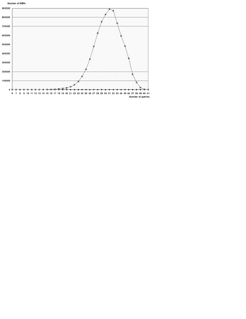
Figure 1: Results of identification of all MBFs of 6 variables

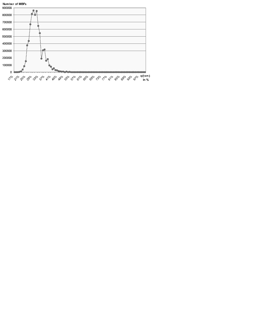
Figure 2: MBFs of 6 variables with one and the same ratio $q/(nm)$ (in %) obtained in their identification

7 Conclusions

In this work we represented our investigations on three important problems, concerning MBFs. We introduced one matrix structure and derived some of its combinatorial and algorithmic properties. They were used as a base for building three algorithms, which was the main reason these problems to be considered from a common point of view. Solving the second and the third problems set some questions, concerning the complexity of the corresponding algorithms, which remained open. They will be subject to our future investigations. We believe that the proposed approach, matrix structure and algorithms have more (and better) properties and capabilities than these, which we succeeded to obtain and represent here.

References

- [1] D. Angluin, Queries and concept learning, Machine learning, 2 (1988) 319–342.
- [2] D. Angluin, L. Hellerstein and M. Karpinski, Learning read-once formulas with queries, J. of the ACM, 40 (1993) 185–210.
- [3] J. C. Bioch, T. Ibaraki, Complexity of identification and dualization of positive Boolean functions, Inform. and Comput., 123 (1995) 50–63.
- [4] E. Boros, P. Hammer, T. Ibaraki, K. Kawakami, Identifying 2-monotonic positive Boolean functions in polynomial time, Lecture Notes in Comp. Sci., 557 (1991) 104–115.
- [5] E. Boros, P. Hammer, T. Ibaraki, K. Kawakami, Polynomial time recognition of 2-monotonic positive Boolean functions given by an oracle, SIAM J. Comput., 26 (1) (1997) 93–109.
- [6] M. Fredman, L. Khachiyan, On the complexity of dualization of monotone disjunctive normal forms, J. of Algorithms, 21 (1996) 618–621.
- [7] D. N. Gainanov, On the criterion of the optimality of an algorithm for evaluating monotonic Boolean functions, USSR Comput. Math. and Math. Physics, 24 (1984) 1250–1257, (or pp. 176–181 in the same issue in English).
- [8] V. Gurvich, L. Khachiyan, On generating the irredundant conjunctive and disjunctive normal forms of monotone Boolean functions, Discrete Appl. Math. 96–97 (1999) 363–373.
- [9] D. Johnson, M. Yannakakis, C. H. Papadimitriou, On generating all maximal independent sets, Inform. Proc. Letters, 27 (1988) 119–123.
- [10] N. Katerincochkina, Searching of the maximal upper zero for one class monotone funcions in -valued logic, Reports of AS USSR, 234 (4) (1977) 746–749, (in Russian).
- [11] G. Kilibarda, V. Yovovic, On the number of monotone Boolean functions with fixed number of lower units, Intellektualnye sistemy, 7 (1–4) (2003) 193–217, (in Russian).
- [12] A. D. Korshunov, On the number of monotone Boolean functions, Problemy Kibernetiki, 38 (1981) 5–108, (in Russian).
- [13] M. Kovalev, P. Milanov, Monotone functions of multivalued logic and supermatroids, USSR Comput. Math. and Math. Physics, 24 (5) (1984) 786-789.
- [14] K. Makino, T. Ibaraki, The maximum latency and identification of positive Boolean functions, SIAM J. Comput., 26 (1997) 1363–1383.
- [15] K. Makino, T. Ibaraki, A fast and simple algorithm for identifying 2-monotonic positive Boolean functions, J. of Algorithms, 26 (1998) 291–305.
- [16] N. A. Sokolov, On the optimal identification of monotone Boolean functions, USSR Comput. Math. and Math. Physics, 22 (2) (1982) 449–461.
- [17] I. Shmulevich, A. Korshunov, J. Astola, Almost all monotone Boolean functions are polynomially learnable using membership queries, Inform. Proc. Letters, 79 (2001) 211–213.
-
[18]
V. Yovovic, G. Kilibarda, On the number of Boolean functions in the Post classes , Discrete Math. and Applications, 9 (1999) 563–586.
Internet references - [19] http://www.angelfire.com/blog/ronz/ – Ron Zeno’s site (Ramblings in mathematics and computer science).
- [20] http://mathpages.com/home/kmath030.htm – Dedekind’s Problem.
-
[21]
https://www.mathpages.com/home/kmath094/kmath094.htm – Generating the
Monotone Boolean Functions. - [22] http://mathpages.com/home/kmath515.htm – Progress on Dedekind’s Problem.
- [23] OEIS Foundation Inc., The On-line Encyclopedia of Integer Sequences. Accessible on-line at https://oeis.org/.