Phase transition in a noisy Kitaev toric code model

Abstract

It is well-known that the partition function of a classical spin model can be mapped to a quantum entangled state where some properties on one side can be used to find new properties on the other side. However, the consequences of the existence of a classical (critical) phase transition on the corresponding quantum state has been mostly ignored. This is particularly interesting since the classical partition function exhibits non-analytic behavior at the critical point and such behavior could have important consequences on the quantum side. In this paper, we consider this problem for an important example of Kitaev toric code model which has been shown to correspond to the two-dimensional (2D) Ising model though a duality transformation. Through such duality transformation, it is shown that the temperature on the classical side is mapped to bit-flip noise on the quantum side. It is then shown that a transition from a coherent superposition of a given quantum state to a non-coherent mixture corresponds exactly to paramagnetic-ferromagnetic phase transition in the Ising model. To identify such a transition further, we define an order parameter to characterize the decoherency of such a mixture and show that it behaves similar to the order parameter (magnetization) of 2D Ising model, a behavior that is interpreted as a robust coherency in the toric code model. Furthermore, we consider other properties of the noisy toric code model exactly at the critical point. We show that there is a relative stability to noise for the toric code state at the critical noise which is revealed by a relative reduction in susceptibility to noise. We close the paper with a discussion on connection between the robust coherency as well as the critical stability with topological order of the toric code model.

I Introduction

Among the well-known connections from classical statistical mechanics to quantum information theory Geraci2008 ; Lidar1997 ; Geraci2010 ; Somma2007 ; Verstraete2006 ; Dennis2002 ; Katzgraber2009 ; ent2006 ; mont2010 ; eis17 ; termo , a fascinating correspondence between partition functions of classical spin models and quantum entangled states has attracted much attention Nest2007 ; algor ; durmar . In 2007, it was shown that the partition function of a classical spin model can be written as an inner product of a product-state and an entangled state Nest2007 . Such mappings led to a cross-fertilization between quantum information theory and statistical mechanics gemma ; Cuevas2011 . Specifically, it has been shown that measurement-based quantum computation (MBQC) on quantum entangled states mqc ; mbqc is related to computational complexity of classical spin models Bravyi2007 ; Bombin2008 . In this way, a new concept of the completeness was defined where the partition function of a classical spin model generates the partition function of all classical models Nest2008 ; Vahid2012b ; Cuevas2009 ; xu ; Vahid2012 ; yahya , see also science ; cub for recent developments in this direction. Most such studies were based on a specific mappings between classical-quantum models. However, we have recently introduced a canonical relation as a duality mapping where any given CSS quantum state can be mapped, via hypergraph representations, to an arbitrary classical spin model zare18 .

On the other hand, the problem of phase transition in classical spin models has attracted much attention in the past and is therefore a well-studied phenomenon stan . Simply, in the high temperature phase such models exhibit no net magnetization due to the symmetric behavior of dynamical variables. Upon decreasing the temperature, this symmetry is spontaneously broken at a critical temperature $T_{cr}$, and a non-zero magnetization appears in the system. The behavior of such systems at the critical point are characterized by non-analytic properties of the leading thermodynamics functions such as magnetic susceptibility. Such non-analytic behavior is characterized by a set of critical exponents which fully identify the symmetry-breaking property (or universality class) of the particular phase transition pathr .

Now, since there is a correspondence between such classical spin models and entangled quantum states, one would have to wonder what the consequences of such phase transitions are on the quantum states. It is our intention to take a step in this direction by considering the well-known ferromagnetic phase transition in a 2D Ising model and its consequences on the Kitaev toric code (TC) Kitaev2003 , which we have previously shown to be related via a duality mapping zare18 . The TC state is of particular interest since it has a topological order wen ; wen2 with a robust nature rob1 ; rob2 ; zare16 ; zareiprb as well as an important application in quantum error correctionerrork ; errorw ; errorb . On the other hand the 2D Ising model is a well-known model in standard statistical mechanics which allows an exact solution. Therefore, one can hope that exploration of such a mapping between the partition function of the Ising model and the TC code can open an avenue for many possible studies related to topological properties of the TC state.

Subsequently, we consider the TC in the presence of an independent bit-flip noise where the Pauli operators $X$ are applied to each qubit with probability $p$. We consider the effect of such a noise in a coherent superposition of two specific quantum states in the TC. Then we define an order parameter that can characterize decoherency of the above quantum state. Interestingly, we show that such an order parameter is mapped to the magnetization of the Ising model. Therefore, we conclude that there is a phase transition from a coherent superposition to a non-coherent mixture of the above quantum state at a critical probability of $p_{cr}$ corresponding to critical temperature of 2D Ising model. We interpret such a behavior as a robust coherency in the TC model. On the other hand, it is well-known that criticality can be marked by interesting behavior at the transition point. Therefore, we define a quantity as susceptibility to noise in the noisy TC model and we show that, at the critical noise of $p_{cr}$, the susceptibility shows a relative reduction which is indicative of critical stability which has been pointed out before zare18 .

This Article is structured as follows: In Sec.(II), we give an introduction to TC model including its ground state and excitations. In Sec.(III), we review the duality mapping from the partition function of 2D Ising model to the TC state and specifically show how such a problem is related to a TC state under a bit-flip noise. In Sec.(IV), we provide our main result where we introduce a decoherence process for a coherent superposition of two quantum state in the TC and we find a singular phase transition to non-coherent phase which is mapped to the ferromagnetic phase transition in the 2D Ising model. In Sec.(V), we introduce a susceptibility to noise which reveals a relative (critical) stability of the toric code state against bit-flip noise at the transition point.

II Review of Kitaev TC model

Toric code (TC) is the first well-known topological quantum code which was introduced by Kitaev in 2003 Kitaev2003 . Since we will consider behavior of this model under noise, here we give a brief review on the TC model which is specifically defined on a 2D square lattice with periodic boundary condition (i.e. on a torus). To this end, consider a $L\times L$ square lattice where qubits live on edges of the lattice. Corresponding to each vertex and face of the lattice, two stabilizer operators are defined in the following form:

$$B_{f}=\prod_{i\in\partial f}X_{i}~{}~{},~{}~{}A_{v}=\prod_{i\in v}Z_{i}$$ (1)

where $i\in\partial f$ refers to all qubits living on edges of the face $f$ and $i\in v$ refers to qubits living on edges incoming to the vertex $v$, see Fig.(1-a). The above operators are in fact generators of the stabilizer group of the TC where each product of them is also a stabilizer. For example, if we represent each face operator of $B_{f}$ as a loop around the boundary of the corresponding face, each product of them will also have a loop representation. In this way, corresponding to each kind of loop in the lattice, there will be an $X$-type stabilizer.

On a torus topology, there are two relations between these operators in the form of $\prod_{f}B_{f}=I$ and $\prod_{v}A_{v}=I$ where $I$ refers to the Identity operator. In this way, the number of independent stabilizers is equal to $2L-2$. By the fact that $[A_{v},B_{f}]=0$, it is simple to show that the following state is an eigenstate of all face and vertex operators with eigenvalue $+1$:

$$|K\rangle=\frac{1}{\sqrt{2^{(|f|-1)}}}\prod_{f}(I+B_{f})|0\rangle^{\otimes 2L}$$

$$=\frac{1}{\sqrt{2^{(|v|-1)}}}\prod_{v}(I+A_{v})|+\rangle^{\otimes 2L}$$ (2)

where $\prod_{f}$ refers to product of all independent face operators and $\prod_{v}$ refers to product of all independent vertex operators. $|f|$ and $|v|$ refer to the number of faces and vertices, respectively. $|0\rangle$ and $|+\rangle=\frac{1}{\sqrt{2}}(|0\rangle+|1\rangle)$ are positive eigenstates of Pauli operators $Z$ and $X$, respectively. The stabilizer space of the toric code is four-fold degenerate and thus there are three other stabilizer states which are generated by non-local operators. In fact, one can consider two non-trivial loops around the torus in two different directions, see Fig.(1-b). Then two operators corresponding to non-trivial loops $\gamma$ and $\gamma^{\prime}$ are defined in the following form:

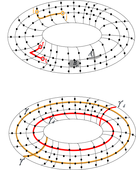
Figure 1: (Color online) a) A 2D square lattice on a torus where qubits live on edges of the lattice. Each vertex (face) operator $A_{v}$ ($B_{f}$) is defined corresponding to each vertex (face) of the lattice. b) There are two different direction on the lattice where two non-trivial loops can be defined. The two non-trivial loops on the edges of the lattice are denoted by $\gamma$ and $\gamma^{\prime}$ while on the dual lattice they are denoted by $\gamma_{d}$ and $\gamma^{\prime}_{d}$.

$$\Gamma_{x}=\prod_{i\in\gamma}X_{i}~{}~{}~{},~{}~{}~{}\Gamma^{\prime}_{x}=\prod_{i\in\gamma^{\prime}}X_{i}$$ (3)

where $i\in\gamma$ and $i\in\gamma^{\prime}$ refers to all qubits living in these loops. In this way, the following four quantum states will be the bases of stabilizer space:

$$|\psi_{\mu,\nu}\rangle=(\Gamma_{x})^{\mu}(\Gamma^{\prime}_{x})^{\nu}|K\rangle~{},$$ (4)

where $\mu,\nu=0,1$ refer to exponent of non-trivial loop operators. In addition to the above non-local operators, there are also two other non-local operators constructed by $Z$ operators. Such operators correspond to two loops $\gamma_{d}$ and $\gamma^{\prime}_{d}$ around the torus on dual lattice in the form of $\Gamma_{z}=\prod_{i\in\gamma_{d}}Z_{i}$ and $\Gamma^{\prime}_{z}=\prod_{i\in\gamma^{\prime}_{d}}Z_{i}$, see Fig.(1-b). One can check that these operators can characterize four different bases of stabilizer space where expectation values of these operators are different for the bases (4).

Another important property of the TC state is related to excitations of the model. To this end, consider two vertices of the lattice denoted by $i$, $j$ where a string, denoted by $S_{ij}$, can connect these two vertices, see Fig.(1-a). Then we apply the Pauli operators $X$ on all qubits belonging to the string $S_{ij}$ where we denote the corresponding string operator by $S_{ij}^{x}$. It is clear that such an operator commutes with all vertex operators $A_{v}$ instead of $A_{i}$ and $A_{j}$, which are the two end-points of the string $S_{ij}$. Such an excited state can also be interpreted as two charge anyons at the two end-points of $S_{ij}$. Charge anyons are generated as pairs and one can move one of them in the lattice by applying a chain of Pauli operators. Furthermore, we can also define string operators of the Pauli operators $Z$. To this end, consider two faces $r$ and $t$ where a string $S_{rt}$ can connect them, see Fig.(1-a). One can define a string operator $S_{rt}^{z}$ which is a product of $Z$ operators on the $S_{rt}$. Similarly, such an operator does not commute with two face operators $B_{r}$ and $B_{t}$ at the two end-points of the $S_{rt}$, and it is interpreted as two flux anyons at the end-points of the $S_{rt}$.

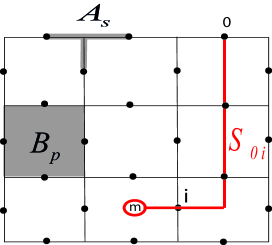
Figure 2: (Color online) TC model on a 2D square lattice with open boundary. The vertex operators corresponding to vertices on the boundary are three-local. If a string start in the boundary the corresponding operator generates only one flux anyon at the end-point of the string in the lattice.

We should emphasize that TC model can also be defined on other lattices with different topologies. The most important difference between different topologies is related to degeneracy of the stabilizer space. Specifically in this paper, we consider a two dimensional square lattice with an open boundary condition, see Fig.(2). Vertex and face operators are defined similar to Eq.(1). However, note that vertex operators corresponding to vertices of the boundary of the lattice are three-body local. It is simple to check that unlike the TC on torus, there is only one constraint on vertex operators, $\prod_{v}A_{v}=I$, and no constraint on face operators. In this way, the degeneracy of stabilizer space will be equal to two. It is also interesting to consider excitation of this model. Unlike the TC on a torus, here one can find flux anyons in odd numbers. In fact if we apply a $Z$ operator on a qubit on the boundary of the lattice it will only generate one flux anyon in the neighboring face. The other flux anyon always lives on the boundary of the lattice. In the other words, the corresponding string operator has two end-points with one on the boundary and another inside the lattice. We denote such a string operator by $S_{0i}$ where $0$ refers to a qubit on the boundary and $i$ refers to a qubit inside the lattice, see Fig.(2).

III Mapping the Ising model to a noisy TC model

It is well-known that the partition function of a classical spin model can be mapped to an inner product of a product state and an entangled state Nest2007 . We have recently provided such a mapping using a duality transformation for CSS states which are mapped to classical spin models zare18 . In this section, we review such mapping between the TC state and 2D Ising model. We also show how a change of variable allows the temperature in the Ising model to be transformed to bit-flip noise in the TC state. To this end, we start with the partition function of a 2D Ising model which is defined on a 2D square lattice with an open boundary condition where we suppose all spins in the boundary are fixed to value of $+1$. The partition function will be in the following form:

$$\mathcal{Z}=\sum_{\{\sigma_{i}\}}e^{\beta J\sum_{\langle i,j\rangle}\sigma_{i}\sigma_{j}}$$ (5)

where $\sigma_{i}=\{\pm 1\}$ refers to spin variables which live on vertices of the lattice which we call vertex spins, $J$ refers to coupling constants and $\beta=\frac{1}{k_{B}T}$. Now, we define new spin variables $\xi_{l}$ which live on edges of the square lattice which we call edge spins. In Fig.(3), we show these new spins by green circles. We also define the value of each edge spin $\xi_{l}$ in the form of $\xi_{l}=\sigma_{i}\sigma_{j}$ where $\sigma_{i}$ and $\sigma_{j}$ are two vertex spins which live on two end-points of the edge $l$. In the next step, we re-write the partition function of Eq.(5) in terms of the edge spins $\xi_{l}$ in the following from:

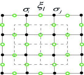
Figure 3: (Color online) Spin variables of the 2D Ising model are denoted by black circles. Corresponding to each edge of the lattice a new spin variable is defined and is denoted by green circle. Dashed lattice is the dual of the initial lattice where faces and vertices of the initial lattice correspond to vertices and faces of the dual lattice, respectively.

$$\mathcal{Z}=\sum_{\{\xi_{l}\}}e^{\beta J\sum_{l}\xi_{l}}\prod_{f}\delta(\prod_{l\in\partial f}\xi_{l})$$ (6)

where $l\in\partial f$ refers to edges around the face of $f$ and we have added delta functions corresponding to each face of the lattice in order to satisfy constraints between edge spins. In other words, since $\xi_{l}=\sigma_{i}\sigma_{j}$, it is clear that the product of spin variables corresponding to each face of the lattice will be equal to one. We should emphasize that one can find another representation for constraints based on dual lattice which is the same as square lattice. As it is shown in Fig.(3), each face of the square lattice corresponds to a vertex of the dual lattice. In this way, constraints in the form of $\prod_{f}\delta(\prod_{l\in\partial f}\xi_{l})$ in Eq.(6) can be replaced by $\prod_{v_{d}}\delta(\prod_{l\in v_{d}}\xi_{l})$ where $v_{d}$ refers to a vertex of the dual lattice. Here, we use such dual representation for finding quantum formalism of 2D Ising model.

Now, we re-write each delta function in the form of $\delta(\prod_{l\in v_{d}}\xi_{l})=\frac{1+\prod_{l\in v_{d}}\xi_{l}}{2}$. Next, the partition function will be written in a quantum language in the following form:

$$\mathcal{Z}=\langle\alpha|G\rangle$$ (7)

where $|\alpha\rangle=(e^{\beta J}|0\rangle+e^{-\beta J}|1\rangle)^{\otimes N_{d}}$ and $|G\rangle=\prod_{v_{d}}\frac{I+\prod_{l\in v_{d}}Z_{l}}{2}(|0\rangle+|1\rangle)^{\otimes N_{d}}$ where $N_{d}$ is the number of edges of the dual lattice. By comparison with Eq.(2) and by the fact that $\prod_{l\in v_{d}}Z_{l}$ is in fact a vertex operator $A_{v}$ on the dual lattice, it is clear that $|G\rangle$ is the same as the toric code state $|K\rangle$ on the dual lattice up to a correction in normalization factor. Finally, the partition function will be in the form of:

$$\mathcal{Z}=\sqrt{2^{|f_{d}|}}\langle\alpha|K\rangle,$$ (8)

where $|f_{d}|$ is the number of faces of the dual lattice. In this way, the partition function of the 2D Ising model on a square lattice is related to a TC state on the dual lattice with qubits which live on the edges.

Now, let us define a new quantity $p$ which is related to Boltzmann weight in the form of $p=\frac{e^{-2\beta J}}{1+e^{-2\beta J}}$. Since $\beta J$ is a quantity between zero to infinity, it is concluded that $0<p<\frac{1}{2}$. In terms of this new quantity, the partition function can be re-written in the following form:

$$\mathcal{Z}=\frac{1}{[p(1-p)]^{\frac{N_{d}}{2}}}W(p),$$ (9)

where

$$W(p)=2^{N_{d}-1}~{}^{N_{d}\otimes}\langle 0|\prod_{i}((1-p)I+pX_{i})|K\rangle.$$ (10)

We now show that the $W(p)$ can be interpreted as an important quantity in a noisy TC state. To this end, we consider a probabilistic bit-flip noise on the TC state where an $X$ operator is applied on each qubit with a probability of $p$. We consider density matrix of the model after applying a quantum channel corresponding to the bit-flip noise. Such a noise leads to different patterns of errors constructed by $X$ operators on qubits and we denote such an error by $\hat{\mathcal{E}}(X)$. The probability of such an error is equal to $W_{\mathcal{E}}(p)=p^{|\mathcal{E}|}(1-p)^{N_{d}-|\mathcal{E}|}$ where $|\mathcal{E}|$ refers to the number of qubits which have been affected by the noise and $N_{d}$ is the total number of qubits. The effect of bit-flip noise on an arbitrary N-qubit quantum state, denoted by density matrix $\rho$, can be presented by a quantum channel in the following form:

$$\Phi(\rho)=\sum_{\mathcal{E}}W_{\mathcal{E}}(p)\hat{\mathcal{E}}(X)\rho\hat{\mathcal{E}}(X)$$ (11)

Now, we come back to the relation of $W(p)$ in Eq.(10) and suppose $p$ as the probability of bit-flip noise. If we expand $\prod_{i}((1-p)I+pX_{i})$ in this equation, we will have a superposition of all possible errors with the corresponding probability in the following form:

$$\prod_{i}((1-p)I+pX_{i})=\sum_{\mathcal{E}}W_{\mathcal{E}}(p)\hat{\mathcal{E}}(X).$$ (12)

On the other hand, the toric code state on the dual lattice is in the form of $|K\rangle=\frac{1}{\sqrt{2^{|f_{d}|}}}\prod_{f}(I+B_{f})|0\rangle^{\otimes N_{d}}$ where the operator $\prod_{f}(I+B_{f})$ is also a superposition of all possible $X$-type loop operators if we interpret the Identity operator as a loop operator with a zero length (an interpretation that will be supposed in the following of the paper). Therefore, it will be easy to see that $W(p)$ is equal to the probability of generating loops in the noisy TC state. By this fact, the Eq.(9) is a relation between partition function of Ising model on a 2D square lattice and the probability of generating loops in the noisy TC state.

IV phase transition in a noisy TC model

Eq.(9) shows that there is a relation between 2D Ising model and a noisy TC state. Since in the 2D Ising model it is well-known that there is phase transition at a critical temperature $T_{cr}$, one can ask if there is a phase transition in the noisy TC model at a corresponding probability of $p_{cr}$. In this section, we consider this problem where we start with magnetization of 2D Ising model and find its quantum analogue in the noisy TC model. Then we show that such a quantum analogue is in fact an order parameter in the noisy TC model which characterizes a transition from a coherent to a non-coherent phase.

We start by considering the mean value of the product of two arbitrary spins in 2D Ising model, i.e. the correlation function. The correlation function is formally given by:

$$\langle\sigma_{m}\sigma_{n}\rangle=\frac{1}{\mathcal{Z}}\sum_{\{\sigma_{i}\}}\sigma_{m}\sigma_{n}e^{\beta J\sum_{\langle i,j\rangle}\sigma_{i}\sigma_{j}}$$ (13)

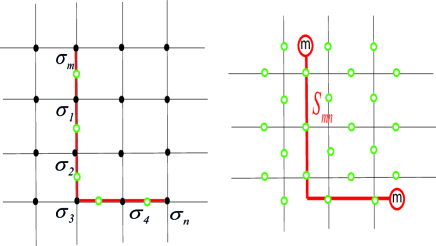
Figure 4: (Color online) Left: There is a chain of spins $\sigma_{1}$, $\sigma_{2}$, $\sigma_{3}$ and $\sigma_{4}$ between two spins $\sigma_{m}$ and $\sigma_{n}$ . Right: after change of variables and converting to quantum language, there will be a string operator corresponding to the initial string $S_{mn}$.

Now, let us consider two particular spins as is shown in Fig.(4). Then we consider an arbitrary string of spins denoted by $S_{mn}$ between two spins $\sigma_{m}$ and $\sigma_{n}$ which we denote by $\sigma_{1},...,\sigma_{4}$. Since $\sigma_{i}^{2}=1$, we can write $\sigma_{m}\sigma_{n}=(\sigma_{m}\sigma_{1})(\sigma_{1}\sigma_{2})(\sigma_{2}\sigma_{3})(\sigma_{3}\sigma_{4})(\sigma_{4}\sigma_{n})$. Next, we write Eq.(13) in the following form:

$$\langle\sigma_{m}\sigma_{n}\rangle=$$

$$\frac{\sum_{\{\sigma_{i}\}}(\sigma_{m}\sigma_{1})(\sigma_{1}\sigma_{2})(\sigma_{2}\sigma_{3})(\sigma_{3}\sigma_{4})(\sigma_{4}\sigma_{n})e^{\beta J\sum_{\langle i,j\rangle}\sigma_{i}\sigma_{j}}}{\mathcal{Z}}$$ (14)

By this new form, we can use edge spins that we defined in the previous section to rewrite the above relation in terms of edge spins $\xi_{l}$. We will have:

$$\langle\sigma_{m}\sigma_{n}\rangle=\frac{1}{\mathcal{Z}}\sum_{\{\xi_{l}\}}[\prod_{l\in S_{mn}}\xi_{l}]~{}~{}e^{\beta J\sum_{l}\xi_{l}}\prod_{f}\delta(\prod_{l\in\partial f}\xi_{l})$$ (15)

where $l\in S_{mn}$ refers to all edges belonging to the string of $S_{mn}$. Similar to procedure that we performed for partition function of 2D Ising model, we can re-write the above relation in a quantum language where we replace edge spins with the Pauli matrices $Z$ and by using definition of TC states, we will have:

$$\langle\sigma_{m}\sigma_{n}\rangle=\frac{\langle\alpha|\prod_{l\in S_{mn}}Z_{l}|K\rangle}{\langle\alpha|K\rangle}=\frac{\langle\alpha|S_{mn}^{z}|K\rangle}{\langle\alpha|K\rangle}$$ (16)

where $S_{mn}^{z}$ is a $Z$-type string operator between vertices of $m$ and $n$ and $S_{mn}^{z}|K\rangle$ is an excited state including two flux anyons in vertices of $m$ and $n$.

The above process can also be applied for mean value of an arbitrary spin of the 2D Ising model denoted by $\langle\sigma_{i}\rangle$ which is in fact the order parameter of this model. Since we considered a 2D Ising model with an open boundary condition where all spins in the boundary of the lattice are fixed to the value of $+1$, expectation value of an arbitrary spin $\sigma_{i}$ is in fact equal to correlation function between that spin and another spin on the boundary of the lattice denoted by $\sigma_{0}=+1$. Therefore, we can use the above formalism for the correlation function to find a quantum formalism for $\langle\sigma_{i}\rangle$.

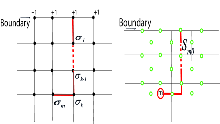
Figure 5: (Color online) Left: There is a chain of spins between boundary of the lattice and spin $\sigma_{m}$. Right: After change of variables and converting to the quantum language, there will be a string operator corresponding to the string of $S_{0m}$ which corresponds to a flux anyon in the TC model with an open boundary.

As we show in Fig.(5), we consider a string of spins $\sigma_{1},...,\sigma_{k}$ between a particular spin $\sigma_{m}$ and a spin $\sigma_{0}=+1$ on the boundary of the lattice. In this way, we will have $\sigma_{m}=(\sigma_{m}\sigma_{1})(\sigma_{1}\sigma_{2})...(\sigma_{k-1}\sigma_{k})(\sigma_{k}\sigma_{0})$ and the order parameter will be in the following form:

$$\langle\sigma_{m}\rangle=$$

$$\frac{\sum_{\{\sigma_{i}\}}(\sigma_{m}\sigma_{1})(\sigma_{1}\sigma_{2})...(\sigma_{k-1}\sigma_{k})(\sigma_{k}\sigma_{0})e^{\beta J\sum_{\langle i,j\rangle}\sigma_{i}\sigma_{j}}}{\mathcal{Z}}$$ (17)

Then we use a change of variable to edge spins $\xi_{l}$ and finally the above equation is re-written in a quantum language in the following form:

$$\langle\sigma_{m}\rangle=\frac{\langle\alpha|\prod_{l\in S_{m0}}Z_{l}|K\rangle}{\langle\alpha|K\rangle}=\frac{\langle\alpha|S_{m0}^{z}|K\rangle}{\langle\alpha|K\rangle}$$ (18)

where $S_{m0}$ refers to a string with one of its end-points on the boundary of the lattice and the other on the face of $m$. Furthermore, since $S_{m0}^{z}$ is an Z-type string operator, the quantum state of $S_{m0}^{z}|K\rangle$ is an excited state of the TC model with only one flux anyon in one of the end-points of the string.

In order to relate the above result to a noisy TC model, we use the transformation from Boltzmann weights in the $|\alpha\rangle$ to probability of noise $p$ according to $p=\frac{e^{-2\beta J}}{1+e^{-2\beta J}}$. In this way, according to Eq.(9) in the previous section, it is clear that the denominator in Eq.(18) is the same as the partition function up to a factor $\sqrt{2^{|f_{d}|}}$ and will in fact be equal to $\frac{W(p)}{\sqrt{2^{|f_{d}|}}[p(1-p)]^{\frac{N_{d}}{2}}}$. Furthermore, we need to find an interpretation for the numerator of Eq.(18). To this end, we note that after transformation to probability of noise $p$, the numerator is written in the following form:

$$\langle\alpha|S_{m0}^{z}|K\rangle=\frac{{}^{N\otimes}\langle 0|(pX+(1-p)I)^{\otimes N}S_{m0}^{z}|K\rangle}{\sqrt{2^{|f_{d}|}}[p(1-p)]^{\frac{N}{2}}}$$ (19)

where we have replaced the $N_{d}$ by $N$ for simplifying the notation. As noted previously, $(pX+(1-p)I)^{\otimes N}$ is equal to superposition of all possible bit-flip errors. On the other hand, in the $S_{m0}^{z}|K\rangle=S_{m0}^{z}\prod_{f}(I+B_{f})|0\rangle^{\otimes N}$, $\prod_{f}(I+B_{f})$ is equal to superposition of all X-type loop operators with the same weight $+1$. However, the string operator $S_{m0}^{z}$ does not commute with $X$-type loop operators that cross the string of $S_{m0}$ odd number of times. Therefore, one can conclude that in the state of $S_{m0}^{z}|K\rangle$ we will have a superposition of all $X$-type loop operators with two different weights $+1$ for loops that cross the string $S_{m0}$ even number of times and $-1$ for loops that cross the $S_{m0}$ odd number of times. By this fact, the numerator will be related to the total probability, denoted by $W_{+}(p)$, that noise leads to loops with even crossings with the $S_{m0}$ minus total probability, denoted by $W_{-}(p)$, that noise leads to loops with odd crossings with $S_{m0}$. Finally, Eq. (18) will be in the following form:

$$\langle\sigma_{m}\rangle=\frac{W_{+}(p)-W_{-}(p)}{W_{+}(p)+W_{-}(p)}$$ (20)

where, we have replaced $W(p)$ in the denominator by $W_{+}(p)+W_{-}(p)$ and we have removed a factor of $\frac{1}{\sqrt{2^{|f_{d}|}}[p(1-p)]^{\frac{N}{2}}}$ from denominator and nominator.

In the above relation on the left hand side, we have the order parameter of the 2D Ising model and the right hand is a quantity related to the noisy toric code state. Now we need to find a physical interpretation for this quantity. Specifically, it will be interesting to show that the right hand side is an order parameter in the noisy TC which characterizes a type of phase transition. To this end, we come back to the noisy model and we consider the effect of the bit-flip noise on a particular initial state. Suppose that the initial state is an eigenstate of string operator $S_{m0}^{z}$. It is simple matter to check that such a state will be in the following form:

$$|\psi_{+}\rangle=\frac{1}{\sqrt{2}}(|K\rangle+S_{mo}^{z}|K\rangle)$$ (21)

The above state is in fact a coherent superposition of a vacuum state $|K\rangle$, where there is no anyon, and a two anyon state $S_{m0}^{z}|K\rangle$ where one lives on the boundary $0$ and the other on the face of $m$. Our main purpose is to investigate the decoherence process of this coherent superposition as a result of noise. We expect that by increasing the probability of the bit flip noise, the initial state converts to a complete mixture of $|K\rangle\langle K|$ and $S_{m0}^{z}|K\rangle\langle K|S_{m0}^{z}$. However, the actual trend, as a function of noise probability, that such a transition to decoherence occurs is an important consideration. For example, is the transition a gradual one or is there a second-order transition? How can one characterize such a transition. Next, we set out to show that such a transition is in fact sharp and can be characterized by an order parameter which measures the amount of coherence in the system.

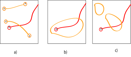
Figure 6: (Color online) Red string refers to the string operator $S_{m0}^{z}$ with a flux anyon in the end-point. a) The first set of errors $E_{1}$ which correspond to open strings of $X$ operators with two charge anyons in the end-points. b) The second set of errors $E_{2}$ which correspond to loops of $X$ operators which cross the $S_{m0}$ odd number of times. C) The third set of errors $E_{3}$ which correspond to loops of $X$ operators which cross the $S_{m0}$ even number of times.

In order to consider the above decoherence process, we divide all errors $\mathcal{E}(X)$ in Eq.(11) to three parts. By the fact that each error of $\mathcal{E}(X)$ can be represented as a pattern of string operators $X$ on the lattice, we consider three kinds of strings which are schematically shown in Fig.(6). The first are open strings where there are charge anyons in the endpoints of those strings. The second are closed strings (loops) that cross the string of $S_{m0}$ odd number of times and the third are closed strings that cross the string of $S_{m0}$ even number of times. It is simple to check that the effect of errors corresponding to the open strings, denoted by $E_{1}$, on the state of $|\psi_{+}\rangle$ leads to generation of charge anyons on endpoints of open strings and takes the initial state to other excited states. The effect of the second kind of errors, denoted by $E_{2}$, is interesting where it takes $|\psi_{+}\rangle$ to $\frac{1}{\sqrt{2}}(|K\rangle-S_{mo}^{z}|K\rangle)$, denoted by $|\psi_{-}\rangle$ which is orthogonal to $|\psi_{+}\rangle$, because loop operators of the second type anti-commute with $S_{m0}^{z}$. Finally the effect of the third kind of errors, denoted by $E_{3}$, is trivial as it takes $|\psi_{+}\rangle$ to $|\psi_{+}\rangle$. In this way, Eq.(11), when we insert $\rho=|\psi_{+}\rangle\langle\psi_{+}|$, can be written in the following form:

$$\Phi(|\psi_{+}\rangle\langle\psi_{+}|)=\sum_{\mathcal{E}\in E_{1}}W_{\mathcal{E}}(p)|\psi_{\mathcal{E}}\rangle\langle\psi_{\mathcal{E}}|$$

$$+W_{-}(p)|\psi_{-}\rangle\langle\psi_{-}|+W_{+}(p)|\psi_{+}\rangle\langle\psi_{+}|$$ (22)

where

$$W_{-}(p)=\sum_{\mathcal{E}\in E_{2}}W_{\mathcal{E}}(p),$$

$$W_{+}(p)=\sum_{\mathcal{E}\in E_{3}}W_{\mathcal{E}}(p)$$

and

$$|\psi_{\mathcal{E}}\rangle=\mathcal{E}(X)|\psi\rangle,$$

and $E_{1}$, $E_{2}$ and $E_{3}$ refer to the above three kinds of errors, respectively. $W_{+}$ and $W_{-}$ are total probability of generating loops which cross the $S_{m0}$ even and odd number of times, respectively. In order to find a better interpretation for the above state, note that in the final quantum state there is a mixture of $|\psi_{+}\rangle$ with probability of $W_{+}(p)$ and $|\psi_{-}\rangle$ with probability of $W_{-}(p)$. In other words, while the state of $|\psi_{+}\rangle=\frac{1}{\sqrt{2}}(|K\rangle+S_{mo}^{z}|K\rangle)$ is a coherent superposition of states $|K\rangle$ and $S_{m0}^{z}|K\rangle$, the effect of bit-flip noise has led to generating a non-coherent mixture of them which can be represented in the corresponding subspace in the following form:

$$\frac{1}{2}\left(\begin{array}[]{cc}(W_{+}+W_{-})&(W_{+}-W_{-})\\ (W_{+}-W_{-})&(W_{+}+W_{-})\\ \end{array}\right)$$ (23)

Now, we need to define a parameter to characterize the amount of decoherency in the above mixture in terms of $p$. According to the Eq.(23), the following parameter is a well-defined measure for the above decoherency:

$$O(p)=\frac{W_{+}(p)-W_{-}(p)}{W_{+}(p)+W_{-}(p)}$$ (24)

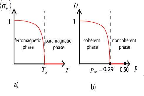
Figure 7: (Color online) a) A schematic representation of the well-known diagram of the order parameter in 2D Ising model where the magnetization goes to zero at $T_{cr}$. b) By comparing Eq.(20) and Eq.(24), the expectation value of the string operator $S_{m0}^{z}$ shows the same behavior with a phase transition at $p_{cr}=0.29$.

This quantity can be also interpreted as the expectation value of $S_{m0}^{z}$ in a subspace which is spanned by $|\psi_{+}\rangle$ and $|\psi_{-}\rangle$. For example, when $W_{+}=W$ and $W_{-}=0$ the order parameter $O$ is equal to $1$ which indicates a coherent superposition and when $W_{+}=W_{-}$, it is equal to $0$ indicating a complete mixture where Eq.(23) becomes proportional to the Identity operator. Now, referring to Eq.(20), we see that $O$ is identical to the order parameter of the 2D Ising model. On the other hand, it is well-known that the order parameter in 2D Ising model characterizes the nature of ferromagnetic phase transition where at a critical temperature $T_{cr}$ system shows a second-order phase transition from ordered phase $\langle\sigma_{m}\rangle\neq 0$ to an disordered phase $\langle\sigma_{m}\rangle=0$. Therefore, by using Eq.(24), it is concluded that there is a phase transition in the noisy TC state where a relatively coherent state, $O\neq 0$ goes to a complete mixture, $O=0$, at a well defined (and relatively large) noise value of $p_{cr}$ which is easily calculated from the critical temperature of the 2D Ising model to be $p_{cr}=0.29$.

The picture that emerges is very interesting. One would expect that increasing bit-flip noise on a coherent superposition would lead to decoherency. However, we have shown that the system remains relatively robust to such an effect for small values of noise probability $p\ll p_{cr}$ and that the transition can be characterized by an order parameter which shows a second-order phase transition to decoherency at a relatively large value of noise value. Fig.(7) schematically shows such a behavior as increasing $p$ from zero to half leads to decoherency at the value of $p_{cr}=0.29$. This interesting and unexpected property indicates a robust coherency which might be related to topological order of the TC state, a point that we will come back to in the Sec.(VI).

V Susceptibility and critical stability at phase transition

Although the existence of a phase transition in a physical system is very important by itself, the critical point which separates two different phases of the system is also a key matter which should specifically be considered. Therefore, we intend to look for other consequences of criticality on the classical side for the quantum model. In this section we consider this problem and specifically show that the ground state of the TC model under the noise displays an interesting behavior precisely at the critical point $p_{cr}$.

We consider an important issue that has been previously emphasized in the general context of CSS states, i.e. relative critical stability, which occurs at $p_{cr}$ zare18 . Here, we investigate such a concept in terms of a susceptibility to noise which is defined for an initial state affected by a bit-flip noise. To this end, we use a familiar quantity in the quantum information theory called fidelity. In other word, if we consider the state of $|K\rangle$ as an initial state, the fidelity of this state and the final state after applying noise will be in the following form:

$$F(p)=\langle K|\Phi(\rho)|K\rangle$$ (25)

where $\Phi(\rho)$ is the final state after applying the bit-flip channel to the initial state $\rho=|K\rangle\langle K|$. Now it is clear that if $F(p)$ is small (large) it means that susceptibility to noise is high (low) because the final state is very different from (similar to) the initial state. In other words, there is an inverse relation between susceptibility to noise and fidelity. Therefore, we define the following quantity to measure the susceptibility:

$$\chi(p)=-Log(F(p)).$$ (26)

It will be interesting to give a physical picture to this quantity. To this end, we interpret $F(p)$ in an anyonic picture for the TC state. In fact, when a bit-flip noise is applied to a qubit of the lattice, it generates two charged anyons. Therefore, the effect of probabilistic bit-flip noise on all qubits can lead to two events, generation of pair anyons and walking anyons in the lattice. It is clear that as long as there is an anyon in the lattice, the system is in an excited mode and fidelity is zero, i.e. susceptibility is infinite. The only possible way that the system comes back to the ground state is that anyons fuse to each other and annihilate. In other words, anyons must generate complete loops in the lattice. This consideration seems to indicate that $F(p)$ should be equal to probability of generating loops which is the same as $W(p)$.

In order to explicitly prove that $F(p)=W(p)$, we use definition of Eq.(25) for $F(p)$. On one hand, we know that $|K\rangle=\frac{1}{\sqrt{{2}^{|f|}}}\prod_{f}(I+B_{f})|0\rangle^{\otimes N}$ and $\prod_{f}(I+B_{f})$ is equal to summation of all possible $X$-type loop operators in the lattice. On the other hand, $\Phi(\rho)$ in Eq.(25) is equal to $\sum_{\mathcal{E}}W_{\mathcal{E}}(p)\hat{\mathcal{E}}(X)\rho\hat{\mathcal{E}}(X)$ which is equal to a summation of all possible $X$-chains with the corresponding probability. In this way, when such a summation inserts between two states $|K\rangle$ in the Eq.(25), all $X$-chains in the summation lead to error and convert the inner product to zero, except for the $X$-chains corresponding to loops which convert the inner product to $1$. Therefore, there will be a summation of probability of generating loops and it is equal to $W(p)$.

Now, we note that $W(p)$ was related to the partition function of 2D Ising model according to Eq.(9) and since $F(p)=W(p)$, we have:

$$\mathcal{Z}=\frac{1}{[p(1-p)]^{\frac{N}{2}}}F(p),$$ (27)

Therefore, one can find the fidelity in the form of $[p(1-p)]^{\frac{N}{2}}\mathcal{Z}$. Since $p\leq\frac{1}{2}$, it is concluded that $[p(1-p)]^{\frac{N}{2}}\rightarrow 0$ for large $N$. In this way, it seems that $F(p)$ should be zero for any non-zero value of $p$ and therefore susceptibility is infinite for any generic noise probability. However, at the critical point, the partition function displays a non-analytic behavior, where fluctuations become relevant. A fluctuation corrections to partition function can be written as pathr :

$$\mathcal{Z}\approx\exp(-\beta A)\sqrt{2\pi kT^{2}C_{v}},$$ (28)

where $A$ is the Helmholtz free energy and $C_{v}$ is the heat capacity which behaves as $C_{v}\sim\mid T-T_{cr}\mid^{-\alpha}$, near the critical point. Fidelity is clearly equal to unity for zero noise (or temperature), but it is also a strongly decreasing function of $p$ as can be seen from Eq.(27). However, the divergence of heat capacity at the critical point will cause a relative increase of the value of fidelity (or relative decrease of susceptibuility) as the critical point is approached, thus leading to a relative stability zare18 .

There are two points about critical stability that should be emphasized. The first is that, the concept of susceptibility that we defined here is not the usual susceptibility in classical phase transitions. For example in the Ising model, heat capacity can be interpreted as susceptibility of the system to an infinitesimal change of temperature. However, in our case, the susceptibility measures stability of the initial state to the whole of the noise not an infinitesimal change of the probability of the noise. In other words, our susceptibility is not defined as a derivative, but as the response of the ground state to a noise probability of finite value $p$.

As the second point, we emphasize that the critical probability of $p_{cr}$ should not be regarded as a threshold for stability of the toric code state. Contrary, it is a relative stability that occurs only at a particular noise probability, $p_{cr}$. It is different from the role of $p_{cr}$ in the previous section where it was a threshold for maintaining coherency of a particular initial state.

A physical picture may help to clarify what is happening in both situations. As $p$ increases the possibility of forming larger loops also increases. It is at $p_{cr}$ where the possibility of having loops of the order of system size, $N$, appear. This is related to the fact that correlation length diverges at the critical point. This system size loops are prime candidates for increasing the value of $W_{-}$, as they are prime candidates for crossing the string operators once, when compared to smaller strings which typically don’t cross or cross twice, see Fig.(6). This explains how the order parameter suddenly drops to zero at the critical point as a significant $W_{-}$ cancels out the already reduced $W_{+}$. Also note that for $p>p_{cr}$, both values of $W_{+}$ and $W_{-}$ are significantly small and equal leading to zero order parameter. On the other hand, the emergence of such system size loops which can occur only at $p_{cr}$, give a relative increase to the value of $W(p)=W_{+}+W_{-}$, thus explaining the relative stability near (at) the critical point.

VI discussion

Although some time has passed since the introduction of quantum formalism for the partition function of classical spin models, it seems that such mappings are richer than what had been previously supposed. In particular, here we studied a neglected aspect of such mappings related to the phase transition on the classical side. In particular, we observed the existence of a sharp transition from a coherent phase to a mixed phase in the noisy TC model as well as a relative critical stability at the transition point. These seem like important physical properties which might find relevance in the applications of quantum states in general. As a closing remark, we would like to emphasize that the large value of the critical noise $P_{cr}=0.29$ can be interpreted as a robust coherency of the initial state against bit-flip noise. On the other hand, since string operators and loop operators in the TC model correspond to processes of generating and fusing anyons, it seems that the robust coherency is in fact related to anyonic properties. This point beside a relative stability at the critical noise support a conjecture that such behaviors might be related to topological order of the TC state. Since, the critical stability has also been observed in other topological CSS states zare18 , it will be interesting to consider the existence of the robust coherency in such models, a problem we intend to address in the future studies.

References

- (1) J. Geraci, D. A. Lidar, “On the exact evaluation of certain instances of the Potts partition function by quantum computers,” Commun. Math. Phys. 279, 735 (2008).
- (2) D. A. Lidar, O. Biham, “Simulating Ising spin glasses on a quantum computer,” Phys. Rev. E 56, 3661 (1997).
- (3) J. Geraci, D. A. Lidar, “Classical Ising model test for quantum circuits,” New J. Phys. 12, 75026 (2010).
- (4) R. D. Somma, C. D. Batista, G. Ortiz, “Quantum approach to classical statistical mechanics,” Phys. Rev. Lett. 99, 030603 (2007).
- (5) F. Verstraete, M. Wolf, D. Perez-Garcia, and J. Cirac, “Criticality, the area law, and the computational power of projected entangled pair states,” Phys. Rev. Lett. 96 (2006).
- (6) E. Dennis, A. Kitaev, A. Landahl, and J. Preskill, “Topological quantum memory,” J. Math. Phys. 43, 4452 (2002).
- (7) H. G. Katzgraber, H. Bombin, M. A. Martin-Delgado, “Error threshold for color codes and random three-body Ising models,” Phys. Rev. Lett. 103, 090501 (2009).
- (8) S. Popescu, A. J. Short, and A. Winter, “Entanglement and the foundations of statistical mechanics.” Nature Physics 2, no. 11 (2006): 754.
- (9) A. Montakhab, A. Asadian, “Multipartite entanglement and quantum phase transitions in the one-, two-, and three-dimensional transverse-field Ising model”, Phys. Rev. A 82, 062313 (2010).
- (10) C. Gogolin, and J. Eisert, “Equilibration, thermalisation, and the emergence of statistical mechanics in closed quantum systems.” Reports on Progress in Physics 79, no. 5 (2016): 056001.
- (11) J. Goold, M. Huber, A. Riera, L. del Rio, and P. Skrzypczyk, “The role of quantum information in thermodynamics—a topical review.” Journal of Physics A: Mathematical and Theoretical 49, no. 14 (2016): 143001.
- (12) M. Van den Nest, W. Dür, H. J. Briegel, “Classical spin models and the quantum-stabilizer formalism,” Phys. Rev. Lett. 98, 117207 (2007).
- (13) M. Van den Nest, W. Dür, R. Raussendorf, and H. J. Briegel, ”Quantum algorithms for spin models and simulable gate sets for quantum computation.” Physical Review A 80, no. 5 (2009): 052334.
- (14) W. Dür, M. Van den Nest, ”Quantum simulation of classical thermal states.” Physical review letters 107, no. 17 (2011): 170402.
- (15) G. De las Cuevas, “A quantum information approach to statistical mechanics.” Journal of Physics B: Atomic, Molecular and Optical Physics 46.24 (2013): 243001.
- (16) G. De las Cuevas, W. Dür, M. Van den Nest and M. A. Martin-Delgado, “Quantum algorithms for classical lattice models,” New J. Phys. 13:093021 (2011).
- (17) R. Raussendorf, H. J. Briegel, “A one-way quantum computer.” Physical Review Letters 86, no. 22 (2001): 5188.
- (18) H. J. Briegel, D. E. Browne, W. Dür, R. Raussendorf, M. Van den Nest, “Measurement-based quantum computation.” Nature Physics, 5(1), 19 (2009).
- (19) S. Bravyi, R. Raussendorf, “Measurement-based quantum computation with the toric code states,” Phys. Rev. A 76, 022304 (2007).
- (20) H. Bombin, M. A. Martin-Delgado, “Statistical mechanical models and topological color codes,” Phys. Rev. A 77, 042322 (2008).
- (21) M. Van den Nest, W. Dür, H. J. Briegel, “Completeness of the classical 2D Ising model and universal quantum computation,” Phys. Rev. Lett. 100, 110501 (2008).
- (22) V. Karimipour. M. H. Zarei, “Algorithmic proof for the completeness of the two-dimensional Ising model,” Phys. Rev. A 86, 052303 (2012).
- (23) G. De las Cuevas, W. Dür, H. J. Briegel, and M. A. Martin-Delgado, “Unifying all classical spin models in a Lattice Gauge Theory,” Phys. Rev. Lett. 102, 230502 (2009).
- (24) Y. Xu, G. De las Cuevas, W. Dür, H. J. Briegel, M. A. Martin-Delgado, “The U (1) lattice gauge theory universally connects all classical models with continuous variables, including background gravity,” J. Stat. Mech. 1102:P02013 (2011).
- (25) V. Karimipour, M. H. Zarei, “Completeness of classical theory on two-dimensional lattices,” Phys. Rev. A 85, 032316 (2012).
- (26) Mohammad Hossein Zarei, Yahya Khalili, “Systematic study of the completeness of two-dimensional classical φ4 theory,” Int. J. Quantum Inform. 15, 1750051 (2017).
- (27) G. De las Cuevas, T. S. Cubitt, “Simple universal models capture all classical spin physics,” Science 351.6278 : 1180-1183 (2016).
- (28) T. S. Cubitt, A. Montanaro, and S. Piddock, “Universal quantum hamiltonians.” Proceedings of the National Academy of Sciences 115, no. 38 (2018): 9497-9502.
- (29) M. H. Zarei, A. Montakhab, “Dual correspondence between classical spin models and quantum CSS states,” Phys. Rev. A 98, 012337 (2018).
- (30) H. E. Stanley, Phase transitions and critical phenomena, Clarendon Press, Oxford, 1971.
- (31) Pathria, R. K. Statistical Mechanics, International Series in Natural Philosophy Volume 45, Pergamon Press, Oxford, UK, 1986.
- (32) A. Y. Kitaev, “Fault-tolerant quantum computation by anyons,” Ann. Phys. (N.Y.) 303, 2 (2003).
- (33) X.-G. Wen, and Q. Niu, “Ground-state degeneracy of the fractional quantum Hall states in the presence of a random potential and on high-genus Riemann surfaces.” Physical Review B 41, no. 13 (1990): 9377.
- (34) X.-G. Wen, “Topological orders and edge excitations in fractional quantum Hall states.” Adv. Phys. 44, 405 (1995).
- (35) S. Trebst, P. Werner, M. Troyer, K. Shtengel, and C. Nayak, “Breakdown of a topological phase: Quantum phase transition in a loop gas model with tension.” Phys. Rev. Lett. 98, 070602 (2007)
- (36) S. Dusuel, M. Kamfor, R. Orus, K. P. Schmidt, and J. Vidal, ”Robustness of a perturbed topological phase.” Physical Review Letters, 106, 107203, (2011).
- (37) M. H. Zarei, ”Robustness of topological quantum codes: Ising perturbation.” Physical Review A 91, no. 2 (2015): 022319.
- (38) Mohammad Hossein Zarei, “strong-weak coupling duality between two perturbed quantum many-body systems: CSS codes and Ising-like systems ,” Phys. Rev. B 96, 165146 (2017).
- (39) E. Dennis, A. Kitaev, A. Landahl, and J. Preskill, “Topological quantum memory.” Journal of Mathematical Physics 43, no. 9 (2002): 4452-4505.
- (40) J. R. Wootton, and J. K. Pachos, “Bringing order through disorder: Localization of errors in topological quantum memories.” Physical review letters 107, no. 3 (2011): 030503.
- (41) B. J. Brown, D. Loss, J. K. Pachos, C. N. Self, and J. R. Wootton. ”Quantum memories at finite temperature.” Reviews of Modern Physics 88, no. 4 (2016): 045005.