Quasiprobability distribution functions from fractional Fourier transforms

Abstract

We show, in a formal way, how a class of complex quasiprobability distribution functions may be introduced by using the fractional Fourier transform. This leads to the Fresnel transform of a characteristic function instead of the usual Fourier transform. We end the manuscript by showing a way in which the distribution we are introducing may be reconstructed by using atom-field interactions.

Keywords: Quasiprobability distribution functions; Fractional Fourier transform; Reconstruction of the wave function.

1 Introduction

It has been already shown that quasiprobability distribution functions may be reconstructed by the measurement of atomic properties in ion-laser interactions [1] and two-level atoms interacting with quantized fields [2, 3]. Such measurements of the wave function are realized usually by measuring atomic observables, namely, the atomic inversion and polarization.

Although the first quasiprobability distribution functions were introduced in the quantum realm [4, 5, 6, 8, 7], they may be also used to analyze classical signals [9, 10].

Ideal interactions, i.e., without taking into account an environment, have shown to lead to the reconstruction of the Wigner function [3] by taking advantage of its expression in terms of the parity operator. However, the interaction of a system with its environment [11] leads to $s$-prametrized quasiprobability distribution functions [12, 13, 14]

$$F(\alpha,s)=\frac{2}{\pi(1-s)}\sum_{k=0}^{\infty}\left(\frac{s+1}{s-1}\right)^{k}\langle k|\hat{D}^{\dagger}(\alpha)\hat{\rho}\hat{D}(\alpha)|k\rangle$$ (1)

where $\hat{D}(\alpha)=\exp(\alpha\hat{a}^{\dagger}-\alpha^{*}\hat{a})$, with $\hat{a}$ and $\hat{a}^{\dagger}$ the annihilation and creation operators of the harmonic oscillator, respectively, is the Glauber displacement operator [15]. The state $\hat{D}(\alpha)|k\rangle=|\alpha,k\rangle$ is a so-called displaced number state [16]. Note that, in order to reconstruct a given quasiprobability function it is needed to do displace the system by an amplitude $\alpha$ and then measure the diagonal elements of the displaced density matrix.

The parameter $s$ defines different orderings and therefore different quasiprobability distribution functions (QDF). The Glauber-Sudarshan $P$-function [15, 17] is given for $s=1$, and is used to obtain averages of functions of normal ordered creation and annihilation operators; $s=-1$ gives the Husimi $Q$-function, used to obtain averages of functions of anti-normal ordered creation and annihilation operators, while $s=0$ is used for the symmetric ordering and gives the Wigner function.

Equation (1) may be rewritten as

$$F(\alpha,s)=\frac{2}{\pi(1-s)}Tr\left\{\left(\frac{s+1}{s-1}\right)^{\hat{a}^{\dagger}\hat{a}}\hat{D}^{\dagger}(\alpha)\hat{\rho}\hat{D}(\alpha)\right\},$$ (2)

that, by using the commutation properties under the symbol of trace, and the system in a pure state $|\psi\rangle$, may be casted into

$$F(\alpha,s) = \frac{2}{\pi(1-s)}Tr\left\{\hat{D}(\alpha)\left(\frac{s+1}{s-1}\right)^{\hat{a}^{\dagger}\hat{a}}\hat{D}^{\dagger}(\alpha)\hat{\rho}\right\}$$ (3)

$$= \frac{2}{\pi(1-s)}\langle\psi|\hat{D}(\alpha)\left(\frac{s+1}{s-1}\right)^{\hat{a}^{\dagger}\hat{a}}\hat{D}^{\dagger}(\alpha)|\psi\rangle.$$

Recent studies have openned the possibility of measuring, instead of observables, non-Hermitian operators [18]. It would be plausible then that such measurements could be related to complex quasiprobability distributions like the McCoy-Kirkwood-Rihaczek-Dirac distribution functions [5, 6, 8, 19].

In this contribution we would like to introduce other kind of complex quasiprobabilities that, although they could be introduced simply by taking $s$ as a complex number, we introduce them in a formal way by considering the fractional Fourier transform (FrFT) [20, 21, 22] of a signal. Then, by writing the Dirac-delta function in terms of its FrFT, we are able to write a general expression for complex quasiprobability distributions in terms of the Fresnel transform. Indeed, the representation of these complex quasiprobability distributions in terms of a Fresnel transform implies that they are solutions of a paraxial wave equation [3]. Finally, by using an effective Hamiltonian for the atom-field interaction, we show how this quasiprobability distribution function may be reconstructed.

2 Fractional Fourier Transform

Up to a phase, the fractional Fourier Transform of a signal $\psi(x)$ can be written by the following expression [20, 21, 22]

$$\mathcal{F}_{\omega}\left[\psi(x)\right]=\exp\left(-i\omega\hat{a}^{\dagger}\hat{a}\right)\psi(x)\;,$$ (4)

that may be expressed in terms of an integral transform as

$$\mathcal{F}_{\omega}\left[\psi(x)\right]=\int_{-\infty}^{+\infty}dx^{\prime}K(x,x^{\prime};\omega)\psi(x^{\prime}),$$ (5)

where

$$K(x,x^{\prime};\omega)=\frac{1}{\sqrt{2\pi i}}\sqrt{\frac{e^{i\omega}}{\sin\omega}}\exp\left[i\frac{x^{2}}{2}\cot\omega+i\frac{x^{\prime 2}}{2}\cot\omega-ixx^{\prime}\csc\omega\right]\,.$$ (6)

Then, if we consider equation (6) as a propagator, Dirac’s delta distribution function takes the form

$$\delta(x-x^{\prime}) = \int_{-\infty}^{+\infty}dx^{\prime\prime}K(x,x^{\prime\prime};-\omega)K(x^{\prime\prime},x^{\prime};\omega)$$ (7)

$$= \frac{1}{2\pi\sin\omega}e^{i\frac{x^{\prime 2}}{2}\cot\omega-i\frac{x^{2}}{2}\cot\omega}\int_{-\infty}^{+\infty}dx^{\prime\prime}e^{ix^{\prime\prime}(x-x^{\prime})\csc\omega}$$

$$= \frac{1}{2\pi}\exp\left[i\frac{x^{\prime 2}}{2}\cot\omega-i\frac{x^{2}}{2}\cot\omega\right]\int_{-\infty}^{+\infty}dx^{\prime\prime}\exp\left[ix^{\prime\prime}(x-x^{\prime})\right]\,.$$

Now, if we apply the fractional Fourier transform to the Dirac delta function we obtain

$$\mathcal{F}_{\omega}\left[\delta(x-y)\right]=\int_{-\infty}^{+\infty}dx^{\prime}K(x,x^{\prime};\omega)\delta(x^{\prime}-y)=K(x,y;\omega).$$ (8)

Then, applying the inverse fractional Fourier transform to equation (8) we obtain an alternative representation of the Dirac delta distribution function

$$\delta(x-y) = \mathcal{F}_{-\omega}\left[\mathcal{F}_{\omega}\left[\delta(x-y)\right]\right]=\int_{-\infty}^{+\infty}dx^{\prime\prime}K(x,x^{\prime\prime};-\omega)K(x^{\prime\prime},y;\omega)$$ (9)

$$= \frac{1}{2\pi}\exp\left[i\frac{y^{2}}{2}\cot\omega-i\frac{x^{2}}{2}\cot\omega\right]\int_{-\infty}^{+\infty}dx^{\prime}\exp\left[ix^{\prime}(x-y)\right]\,.$$

From the above equation it may be seen that there is a phase multiplying the usual integral representation of the Dirac delta function, that although could be omitted by using properties of the delta function, we keep in order to obtain a quasiprobability distribution function as a fractional Fourier (Fresnel) transform of the characteristic function.

3 Probability distribution in the phase space

We define $J(q,p)$ a probability distribution in the phase space as

$$J(q,p)=\int_{-\infty}^{+\infty}\int_{-\infty}^{+\infty}dq^{\prime}dp^{\prime}\mathcal{P}(q^{\prime},p^{\prime})\delta(q^{\prime}-q)\delta(p-p^{\prime})\,,$$ (10)

then, using equation (9), the distribution $J(q,p)$ may be rewritten as

$$J(q,p) = \frac{1}{4\pi^{2}}e^{i\frac{q^{2}}{2}\cot\alpha-i\frac{p^{2}}{2}\cot\beta}\int_{-\infty}^{+\infty}\int_{-\infty}^{+\infty}dudv\,e^{iup-ivq}\,\times$$ (11)

$$\times {Tr}\left\{\hat{\rho}e^{iv\hat{q}-iu\hat{p}+i\frac{\hat{p}^{2}}{2}\cot\beta-i\frac{\hat{q}^{2}}{2}\cot\alpha}\right\}\,,$$

and because

$$e^{iv\hat{q}-iu\hat{p}+i\frac{\hat{p}^{2}}{2}\cot\beta-i\frac{\hat{q}^{2}}{2}\cot\alpha} = e^{-i\frac{u^{2}}{2}\tan\beta}e^{i\frac{v^{2}}{2}\tan\alpha}e^{iu\tan\beta\hat{q}}e^{-iv\tan\alpha\hat{p}}\times$$ (12)

$$\times e^{i\frac{\hat{p}^{2}}{2}\cot\beta-i\frac{\hat{q}^{2}}{2}\cot\alpha}e^{iv\tan\alpha\hat{p}}e^{-iu\tan\beta\hat{q}}\,,$$

equation (11) takes the form

$$J(q,p) = \frac{1}{4\pi^{2}}e^{i\frac{q^{2}}{2}\cot\alpha-i\frac{p^{2}}{2}\cot\beta}\int_{-\infty}^{+\infty}\int_{-\infty}^{+\infty}dudv\,e^{iup-ivq}e^{-i\frac{u^{2}}{2}\tan\beta}e^{i\frac{v^{2}}{2}\tan\alpha}\,\times$$ (13)

$$\times Tr\left\{\hat{\rho}e^{iu\tan\beta\hat{q}}e^{-iv\tan\alpha\hat{p}}e^{i\frac{\hat{p}^{2}}{2}\cot\beta-i\frac{\hat{q}^{2}}{2}\cot\alpha}e^{iv\tan\alpha\hat{p}}e^{-iu\tan\beta\hat{q}}\right\}\,,$$

that by using the equivalence

$$e^{iu\tan\beta\hat{q}}e^{-iv\tan\alpha\hat{p}}=e^{\frac{i}{2}uv\tan\alpha\tan\beta}e^{iu\tan\beta\hat{q}-iv\tan\alpha\hat{p}}\,,$$ (14)

may be casted into the expression

$$J(q,p) = \frac{1}{4\pi^{2}}\,e^{i\frac{q^{2}}{2}\cot\alpha-i\frac{p^{2}}{2}\cot\beta}\int_{-\infty}^{+\infty}\int_{-\infty}^{+\infty}dudv\,e^{iup-ivq}e^{-i\frac{u^{2}}{2}\tan\beta}e^{i\frac{v^{2}}{2}\tan\alpha}\,\times$$ (15)

$$\times Tr\left\{\hat{\rho}e^{iu\tan\beta\hat{q}-iv\tan\alpha\hat{p}}e^{i\frac{\hat{p}^{2}}{2}\cot\beta-i\frac{\hat{q}^{2}}{2}\cot\alpha}e^{iv\tan\alpha\hat{p}-iu\tan\beta\hat{q}}\right\}\,.$$

3.1 Case $\cot\alpha=-\cot\beta=\pi$

The above quasiprobability distribution function is defined for a range of parameters $\alpha$ and $\beta$, however, for the sake of simplicity, we will consider the case $\cot\alpha=-\cot\beta=\pi$.

We may relate the quasiprobability distribution function $J(q,p)$ to the Wigner function, by noting that, for $\cot\alpha=-\cot\beta=\pi$, equation (15) has the form

$$J(q,p) = \frac{1}{4\pi^{2}i}e^{i\pi\left(\frac{p^{2}}{2}+\frac{q^{2}}{2}\right)}\int_{-\infty}^{+\infty}\int_{-\infty}^{+\infty}dudv\,e^{iup-ivq}e^{i\frac{u^{2}}{2\pi}+i\frac{v^{2}}{2\pi}}\times$$ (16)

$$\times Tr\left\{\hat{\rho}e^{-i\frac{u\hat{q}}{\pi}-i\frac{v\hat{p}}{\pi}}(-1)^{\hat{n}}e^{i\frac{u\hat{q}}{\pi}+i\frac{v\hat{p}}{\pi}}\right\}.$$

According to trace representation of Wigner function [14]

$$W\left(\frac{v}{\pi},-\frac{u}{\pi}\right)=Tr\left\{\hat{\rho}\,\frac{1}{\pi}\,e^{-i\frac{u\hat{q}}{\pi}-i\frac{v\hat{p}}{\pi}}(-1)^{\hat{n}}e^{i\frac{u\hat{q}}{\pi}+i\frac{v\hat{p}}{\pi}}\right\},$$ (17)

we write the distribution $J(q,p)$ as the Fresnel transform of the Wigner function

$$J(q,p)=\frac{1}{4\pi i}e^{i\pi\left(\frac{p^{2}}{2}+\frac{q^{2}}{2}\right)}\int_{-\infty}^{+\infty}\int_{-\infty}^{+\infty}dudv\,e^{iup-ivq}e^{i\frac{u^{2}}{2\pi}+i\frac{v^{2}}{2\pi}}W\left(\frac{v}{\pi},-\frac{u}{\pi}\right)\,.$$ (18)

It is easy to show that the quasiprobability distribution (18) can be normalized

$$\int_{-\infty}^{+\infty}\int_{-\infty}^{+\infty}dqdp\,J(q,p)$$

$$=\frac{\pi}{2}\int_{-\infty}^{+\infty}\int_{-\infty}^{+\infty}dxdy\,\left[\frac{1}{2\pi}\int_{-\infty}^{+\infty}dpe^{ixp}\right]\left[\frac{1}{2\pi}\int_{-\infty}^{+\infty}dqe^{-iyq}\right]e^{-i\frac{x^{2}}{2\pi}-i\frac{y^{2}}{2\pi}}Tr\left\{\hat{\rho}\,e^{iy\hat{q}-ix\hat{p}}\right\}$$

$$=\frac{\pi}{2}\int_{-\infty}^{+\infty}\int_{-\infty}^{+\infty}dxdy\,\delta(x)\delta(y)e^{-i\frac{x^{2}}{2\pi}-i\frac{y^{2}}{2\pi}}Tr\left\{\hat{\rho}\,e^{iy\hat{q}-ix\hat{p}}\right\}=\frac{\pi}{2}Tr\left\{\hat{\rho}\right\}=\frac{\pi}{2}\,.$$ (19)

Therefore, for normalization reasons, the quasiprobability distribution is finally given in the form

$$J(q,p)=\frac{1}{4\pi^{2}}\int_{-\infty}^{+\infty}\int_{-\infty}^{+\infty}du\,dv\,e^{iup-ivq}e^{-i\frac{u^{2}}{2\pi}-i\frac{v^{2}}{2\pi}}Tr\left\{\hat{\rho}\,e^{iv\hat{q}-iu\hat{p}}\right\}\,,$$ (20)

that, by applying the change of variables $\beta=u/\sqrt{2}+iv/\sqrt{2}$ takes the form

$$J(\alpha)=\frac{1}{2\pi^{2}}\int d^{2}\beta\,e^{\alpha\beta^{*}-\alpha^{*}\beta}e^{-\frac{i}{\pi}|\beta|^{2}}Tr\left\{\hat{\rho}\,\hat{D}(\beta)\right\}\,,$$ (21)

with $\alpha=q/\sqrt{2}+ip/\sqrt{2}$.

From the above expression it is direct to show that the Wigner function

$$W(\alpha)=\int d^{2}\beta e^{\alpha\beta^{*}-\alpha^{*}\beta}\{\hat{\rho}\hat{D}(\beta)\},$$ (22)

and the function $J(\alpha)$ may be easily related by the differential relation

$$J(\alpha)=\exp\left\{\frac{i}{\pi}\frac{\partial^{2}}{\partial\alpha\partial\alpha^{*}}\right\}W(\alpha).$$ (23)

The above quasiprobability function may be written as a trace by noting that

$$\frac{1}{2\pi^{2}}\int d^{2}\beta\,\exp\left(-\frac{i}{\pi}|\beta|^{2}\right)\hat{D}(\beta)=\frac{1}{2i+\pi}\left(\frac{2i-\pi}{2i+\pi}\right)^{\hat{n}}$$ (24)

that leads to the trace representation of $J(q,p)$

$$J(q,p)=\frac{1}{2i+\pi}Tr\left\{\hat{\rho}\,\hat{D}(\alpha)\,\left(\frac{2i-\pi}{2i+\pi}\right)^{\hat{n}}\,\hat{D}^{\dagger}(\alpha)\right\}\,.$$ (25)

Last equation allows us to show that $J(q,p)$ is correctly normalized, for this we do the double integration

$$\int_{-\infty}^{+\infty}\int_{-\infty}^{+\infty}J(q,p)dqdp = Tr\left\{\hat{\rho}\frac{2}{\pi+2i}\int\,d^{2}\alpha\hat{D}(\alpha)\hat{D}^{\dagger}\left(\alpha e^{i\theta}\right)e^{i\theta\hat{n}}\right\}$$ (26)

$$= Tr\left\{\hat{\rho}\,\hat{A}\,e^{i\theta\hat{n}}\right\}\,,$$

where we have defined

$$e^{i\theta}=\frac{2i-\pi}{2i+\pi}\,,$$ (27)

and

$$\hat{A} = \frac{2}{\pi+2i}\int d^{2}\alpha\,e^{i\sin\theta|\alpha|^{2}}\hat{D}\left(\alpha\left(1-e^{i\theta}\right)\right)$$ (28)

$$= \frac{1}{\pi^{2}}\int\int d^{2}z_{1}d^{2}z_{2}\left|z_{1}\right\rangle\left\langle z_{2}\right|B(z_{1},z_{2},z^{*}_{1},z^{*}_{2})\,,$$

with

$$B(z_{1},z_{2},z^{*}_{1},z^{*}_{2})=\frac{2}{\pi+2i}\int d^{2}\alpha\,e^{i\sin\theta|\alpha|^{2}}\langle z_{1}|\hat{D}\left(\alpha\left(1-e^{i\theta}\right)\right)|z_{2}\rangle$$

$$=\frac{2\langle z_{1}|z_{2}\rangle}{\pi+2i}\int_{-\infty}^{+\infty}\,d\alpha_{x}\exp\left(-\left(1-e^{i\theta}\right)\alpha_{x}^{2}+\alpha_{x}\left(\left(1-e^{i\theta}\right)z^{*}_{1}-\left(1-e^{-i\theta}\right)z_{2}\right)\right)\times$$

$$\times\int_{-\infty}^{+\infty}\,d\alpha_{y}\exp\left(-\left(1-e^{i\theta}\right)\alpha_{x}^{2}+i\alpha_{y}\left(\left(1-e^{i\theta}\right)z^{*}_{1}+\left(1-e^{-i\theta}\right)z_{2}\right)\right)$$

$$=\frac{2\langle z_{1}|z_{2}\rangle}{\pi+2i}\frac{\pi}{1-e^{i\theta}}\left[-\left(1-e^{-i\theta}\right)z^{*}_{1}z_{2}\right]=\left(-\frac{|z_{1}|^{2}}{2}-\frac{\left|z_{2}e^{-i\theta}\right|^{2}}{2}+z^{*}_{1}\left(e^{-i\theta}z_{2}\right)\right)$$

$$=\langle z_{1}|e^{-i\theta\hat{n}}|z_{2}\rangle\,.$$ (29)

By replacing equation (3.1) into equation (28) we obtain

$$\hat{A}=e^{-i\theta\hat{n}}\,,$$ (30)

that shows that equation (26) is correctly normalized

$$\int_{-\infty}^{+\infty}\int_{-\infty}^{+\infty}J(q,p)dqdp=Tr\left\{\hat{\rho}\,e^{-i\theta\hat{n}}\,e^{i\theta\hat{n}}\right\}=Tr\left\{\hat{\rho}\right\}=1\,.$$ (31)

4 Kirkwood distribution and $J(q,p)$ distribution

Being the QDF $J(q,p)$ and Kirkwood distributions complex functions we show now some differences between them.

The Kirkwood distribution is defined as [8, 19, 23, 24]

$$K(q,p)=\frac{1}{4\pi^{2}}\int_{-\infty}^{+\infty}\int_{-\infty}^{+\infty}du\,dv\,e^{iup-ivq}e^{i\frac{uv}{2}}Tr\left\{\hat{\rho}e^{iv\hat{q}-iu\hat{p}}\right\}\,,$$ (32)

or an alternative way to write it as an expectation value [25] is

$$K(q,p)=\frac{1}{\sqrt{2}\pi}e^{\frac{q^{2}}{2}+\frac{p^{2}}{2}+iqp}\langle-i\sqrt{2}p|e^{\frac{\hat{a}^{2}}{2}}\hat{\rho}e^{-\frac{\hat{a}^{\dagger\,2}}{2}}|\sqrt{2}q\rangle.$$ (33)

4.1 Number state

The Kirkwood $K(q,p)$ and $J(q,p)$ distributions for number state $\left|n\right\rangle$, are represented by the following equations

$$K_{n}(q,p)=\frac{i^{n}}{2^{n}n!\pi\sqrt{2}}e^{-\frac{q^{2}}{2}-\frac{p^{2}}{2}+iqp}H_{n}(q)H_{n}(p)$$ (34)

and

$$J_{n}(q,p)=\frac{1}{2i+\pi}\left(\frac{2i-\pi}{2i+\pi}\right)^{n}\exp\left(-\frac{\pi(q^{2}+p^{2})}{2i+\pi}\right)L_{n}\left(\frac{2\pi^{2}(q^{2}+p^{2})}{4+\pi^{2}}\right)\,,$$ (35)

where, $H_{n}(x)$ and $L_{n}(x)$ are Hermite and Laguerre polynomials, respectively.

4.2 Superposition of two coherent states

Now, we consider a superposition of two coherent states as:

$$\left|\psi_{\pm}\right\rangle=\frac{1}{\sqrt{2\pm 2\mathrm{Re}\langle\alpha_{1}|\alpha_{2}\rangle}}\left(\left|\alpha_{1}\right\rangle\pm\left|\alpha_{2}\right\rangle\right)\,,$$ (36)

$$\left|\psi_{\pm}\right\rangle=\frac{1}{\sqrt{2\pm 2\mathrm{Re}\langle\alpha_{1}|\alpha_{2}\rangle}}\left(\left|\alpha_{1}\right\rangle\pm\left|\alpha_{2}\right\rangle\right)\,,$$ (37)

where $\alpha_{k}=q_{k}/\sqrt{2}+ip_{k}/\sqrt{2}$, such that the Kirkwood $K(q,p)$ and the $J(q,p)$ distributions for the superposition of two coherent states, $\left|\psi_{\pm}\right\rangle$, is given by

$$J_{\pm}(q,p)=\frac{1}{2i+\pi}\frac{1}{2\pm 2\mathrm{Re}\langle\alpha_{1}|\alpha_{2}\rangle}\left(\exp\left(-\frac{\pi}{2i+\pi}\left((q-q_{1})^{2}+(p-p_{1})^{2}\right)\right)\right)$$

$$\frac{1}{2i+\pi}\frac{1}{2\pm 2\mathrm{Re}\langle\alpha_{1}|\alpha_{2}\rangle}\left(\exp\left(-\frac{\pi}{2i+\pi}\left((q-q_{2})^{2}+(p-p_{2})^{2}\right)\right)\right)$$

$$\pm\frac{1}{2i+\pi}\frac{1}{2\pm 2\mathrm{Re}\langle\alpha_{1}|\alpha_{2}\rangle}\left(\exp\left(\frac{i}{2}\left(q\left(p_{1}-p_{2}\right)-p\left(q_{1}-q_{2}\right)\right)\right)\langle\alpha_{2}-\alpha|e^{i\theta}(\alpha_{1}-\alpha)\rangle\right)$$

$$\pm\frac{1}{2i+\pi}\frac{1}{2\pm 2\mathrm{Re}\langle\alpha_{1}|\alpha_{2}\rangle}\left(\exp\left(-\frac{i}{2}\left(q\left(p_{1}-p_{2}\right)-p\left(q_{1}-q_{2}\right)\right)\right)\langle\alpha_{1}-\alpha|e^{i\theta}(\alpha_{2}-\alpha)\rangle\right)$$

and

$$K_{\pm}(q,p)=\frac{1}{\sqrt{2}\pi}\frac{\exp\left(-\frac{q^{2}}{2}-\frac{p^{2}}{2}+iqp\right)}{2\pm 2\mathrm{Re}\langle\alpha_{1}|\alpha_{2}\rangle}\exp\left(-\frac{1}{2}(q^{2}_{1}+p^{2}_{1})+(qq_{1}-pp_{1})\right)\times$$

$$\times\exp\left(\frac{i}{2}q_{1}(p_{1}+2p)+\frac{i}{2}p_{1}(q_{1}-2q)\right)$$

$$+\frac{1}{\sqrt{2}\pi}\frac{\exp\left(-\frac{q^{2}}{2}-\frac{p^{2}}{2}+iqp\right)}{2\pm 2\mathrm{Re}\langle\alpha_{1}|\alpha_{2}\rangle}\exp\left(-\frac{1}{2}(q^{2}_{2}+p^{2}_{2})+(qq_{2}-pp_{2})\right)\times$$

$$\times\exp\left(\frac{i}{2}q_{2}(p_{2}+2p)+\frac{i}{2}p_{2}(q_{2}-2q)\right)$$

$$\pm\frac{1}{\sqrt{2}\pi}\frac{\exp\left(-\frac{q^{2}}{2}-\frac{p^{2}}{2}+iqp\right)}{2\pm 2\mathrm{Re}\langle\alpha_{1}|\alpha_{2}\rangle}\exp\left(-\frac{1}{2}(q^{2}_{1}+p^{2}_{2})+(qq_{1}-pp_{2})\right)\times$$

$$\times\exp\left(\frac{i}{2}q_{2}(p_{2}+2p)+\frac{i}{2}p_{1}(q_{1}-2q)\right)$$

$$\pm\frac{1}{\sqrt{2}\pi}\frac{\exp\left(-\frac{q^{2}}{2}-\frac{p^{2}}{2}+iqp\right)}{2\pm 2\mathrm{Re}\langle\alpha_{1}|\alpha_{2}\rangle}\exp\left(-\frac{1}{2}(q^{2}_{2}+p^{2}_{1})+(qq_{2}-pp_{1})\right)\times$$

$$\times\exp\left(\frac{i}{2}q_{1}(p_{1}+2p)+\frac{i}{2}p_{2}(q_{2}-2q)\right)\,,$$ (39)

respectively.

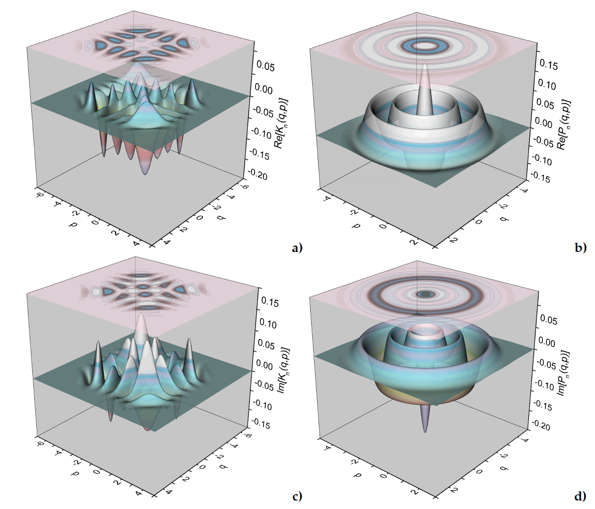
Figure 1: In figures a) and c) we can see the phase space distribution of the real and imaginary parts of the Kirkwood function for a number state $\left|n=3\right\rangle$. In figures b) and d) we see the distribution $J(q,p)$, for the same number state, again, the real and imaginary parts, respectively.

We plot both distribution in Figures 1 and 2. In both figures a more uniform behaviour may be seen in the QDF $J_{\pm}(q,p)$ than in the Kirkwood function. In fact, the real and imaginary parts of the distribution we have introduced here, look like Wigner function for number states (Fig. 1) and Scrhödinger cat states (Fig. 2).

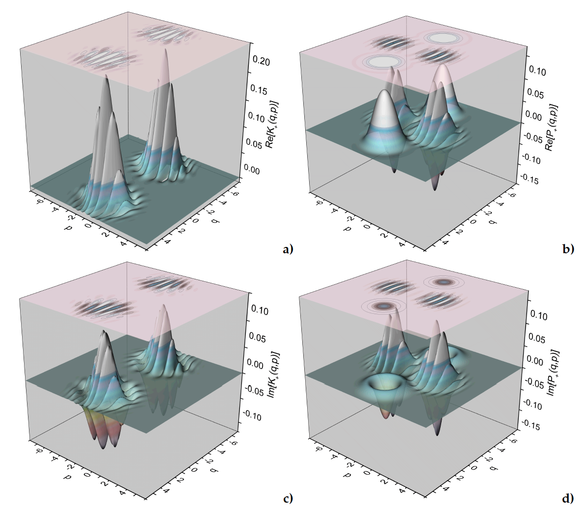
Figure 2: In figures a) and c) we can see the phase space distribution of the real and imaginary parts of the Kirkwood function for two superposition of coherent states $\left|\psi_{+}\right\rangle$ wiht $q_{1}=-q_{2}=4$ and $p_{1}=p_{2}=0$. In figures b) and d) we see the distribution $J(q,p)$, again, the real and imaginary parts, respectively.

5 Reconstruction of distribution $J(\alpha)$

It is not difficult to show that the real part of QDF $J(\alpha)$ may be measured. This can be achieved by measuring the atomic polarization in the dispersive interaction between an atom and a quantized field [3], whose Hamiltonian reads

$$\hat{H}=-\chi\hat{a}^{\dagger}\hat{a}\hat{\sigma}_{z},$$ (40)

with $\hat{\sigma}_{z}=|e\rangle\langle e|-|g\rangle\langle g|$, the Pauli matrix corresponding to the atomic inversion operator, where $|g\rangle$ and $|e\rangle$ represent the ground and excited states of the two-level atom. The parameter $\chi$ is the dispersive coupling constant. The above Hamiltonian yields the evolution operator

$$\hat{U}(t)=\exp\{-i\chi t\hat{a}^{\dagger}\hat{a}\hat{\sigma}_{z}\},$$ (41)

from where we can obtain the evolved wavefunction $|\psi(t)\rangle=\hat{U}(t)|\psi(0)\rangle$, that allows the calculation of averages of different observables.

The average of observable $\hat{\sigma}_{x}=|e\rangle\langle g|+|g\rangle\langle e|$ then can be obtained for an arbitrary initial field, which we conveniently write as $|\psi_{F}(0)\rangle=\hat{D}^{\dagger}(\alpha)|\phi(0)\rangle$ and the atom is initially in a superposition of atomic states, $|\psi_{A}(0)\rangle=\frac{1}{\sqrt{2}}(|g\rangle+|e\rangle)$. Then we write

$$\langle\hat{\sigma}_{x}(t)\rangle=\frac{1}{2}\left(\langle\phi(0)|\hat{D}(\alpha)\exp\{2i\chi t\hat{a}^{\dagger}\hat{a}\}\hat{D}^{\dagger}(\alpha)|\phi(0)\rangle+c.c.\right).$$ (42)

It is also easy to show that the imaginary part of the QDF may be associated to the observable $\hat{\sigma}_{y}=i(|e\rangle\langle g|-|g\rangle\langle e|)$

$$\langle\hat{\sigma}_{y}(t)\rangle=\frac{i}{2}\left(\langle\phi(0)|\hat{D}(\alpha)\exp\{2i\chi ta^{\dagger}a\}\hat{D}^{\dagger}(\alpha)|\phi(0)\rangle-c.c.\right).$$ (43)

If we set the interaction time $t=\frac{\arctan\frac{4\pi}{\pi^{2}-4}}{2\chi}$, we obtain that

$$Re\{J(\alpha)\}\propto\langle\hat{\sigma}_{x}\rangle,\qquad Im\{J(\alpha)\}\propto\langle\hat{\sigma}_{y}\rangle.$$ (44)

Therefore, by measuring the polarizations $\hat{\sigma}_{x}$ and $\hat{\sigma}_{y}$ we are able to measure the QDF $J(\alpha)$.

6 Conclusions

We have introduced a set of parametrized (in terms of $\alpha$ and $\beta$) quasiprobability distribution functions, equation (15), by using the fractional Fourier transform. This has lead us to generalize QDF to Fresnel transforms of the characteristic function instead of their usual Fourier transforms. We have also shown how such QDF may be recosntructed in the dispersive atom-field interaction. We have also given a (differential) relation that allows the calculation of the newly introduced QDF from the Wigner function.

Acknowledgments: We thank CONACYT for support.

References

- [1] D. Leibfried, D. M. Meekhof, B. E. King, C. Monroe, W. M. Itano, and D. J. Wineland, Experimental Determination of the Motional Quantum State of a Trapped Atom, Phys. Rev. Lett. 77, 4281 (1996).
- [2] P. Bertet, A. Auffeves, P. Maioli, S. Osnaghi, T. Meunier, M. Brune, J. M. Raimond, and S. Haroche, Direct Measurement of the Wigner Function of a One-Photon Fock State in a Cavity, Phys. Rev. Lett. 89, 200402 (2002).
- [3] L.G. Lutterbach, and L. Davidovich, Phys. Rev. Lett. 78, 2547 (1997), Method for Direct Measurement of the Wigner Function in Cavity QED and Ion Traps.
- [4] E.P. Wigner,. On the quantum correction for thermodynamic equilibrium. Phys. Rev. 1932, 40, 749.
- [5] N. H. McCoy, On the Function in Quantum Mechanics Which Corresponds to a Given Function in Classical Mechanics. Proc. Natl. Acad. Sci. U.S.A. 18, 674 (1932).
- [6] P.A.M. Dirac, On the Analogy Between Classical and Quantum Mechanics. Rev. Mod. Phys. 17, 195 (1945).
- [7] K. Husimi, Some Formal Properties of the Density Matrix, Proc. Phys. Math. Soc. Jpn. 22, 264–314 (1940).
- [8] J.G. Kirkwood, Quantum Statistics of Almost Classical Assemblies. Phys. Rev. 44, 31-37 (1933).
- [9] Alonso, M. A, Wigner functions in optics: describing beams as ray bundles and pulses as particle ensembles. Advances in Optics and Photonics 3, 272-365 (2011)
- [10] M. J. Bastiaans and K. B. Wolf, Phase reconstruction from intensity measurements in linear systems J. Opt. Soc. Am. A 20, 1046-1049 (2003).
- [11] N. Yazdanpanah, M.K. Tavassoly, R. Juárez-Amaro and H.M. Moya-Cessa, Reconstruction of quasiprobability distribution functions of the cavity field considering field and atomic decays, Opt. Commun. 400, 69-73 (2017).
- [12] A. Royer, Wigner function as the expectation value of a parity operator, Phys. Rev. A 15, 449 (1977).
- [13] A. Wünsche, Displaced Fock states and their connection to quasi-probabilities. Quantum Opt. 3, 359-383 (1991).
- [14] H. Moya-Cessa and P.L. Knight, Series representation of quantum-field quasiprobabilities, Phys. Rev. A 48, 2479 (1993).
- [15] R.J. Glauber, Coherent and Incoherent States of the Radiation Field, Phys. Rev. 131, 2766 (1963).
- [16] F.A.M. de Oliveira, M.S. Kim, P.L. Knight and V. Buzek, Properties of displaced number states, Phys. Rev. A 41, 2645 (1990).
- [17] E.C.G. Sudarshan, Equivalence of Semiclassical and Quantum Mechanical Descriptions of Statistical Light Beams, Phys. Rev. Lett. 10, 277 (1963).
- [18] A.K. Pati, U. Singh and U. Sinha, Measuring non-Hermitian operators via weak values. Phys. Rev. A 92, 052120 (2015).
- [19] A.N. Rihaczek, Signal energy distribution in time and frequency . IEEE Trans. Inf. Theory 14, 369-374 (1968).
- [20] Namias, V. “The Fractional order Fourier transform and its application to quantum mechanics,” J. Inst. Maths. Applics. 25, 241-265 (1980).
- [21] G. S.Agarwal and R. Simon, A simple realization of fractional Fourier transform and relation to harmonic oscillator Green’s function. Opt. Commun. 110, 23 (1994).
- [22] H.-Y. Fan and J.-H. Chen, On the core of the fractional Fourier transform and its role in composing complex fractional Fourier transformations and Fresnel transformations. Front. Phys. 10, 100301 (2015).
- [23] L. Praxmeyer and K. Wódkiewicz, Quantum Interference in the Kirkwood-Rihaczek representation. Opt. Comm. 223, 349-365 (2003).
- [24] L. Praxmeyer and K. Wódkiewicz, Hydrogen atom in phase space: The Kirkwood-Rihaczek representation Phys. Rev. A 67, 054502 (2003).
- [25] H. Moya-Cessa, Relation between the Glauber-Sudarshan and Kirkwood-Rihaczec distribution functions J. Mod. Opt 60, 726-730 (2013).