Study of the $h\gamma Z$ coupling using $e^{+}e^{-}\xrightarrow{}h\gamma$ at the ILC

Abstract

We study the $e^{+}e^{-}\to h\gamma$ process at the International Linear Collider (ILC) to probe new physics in the $h\gamma Z$ coupling. The study is performed at a center of mass energy of 250 GeV and is based on the full simulation of the International Large Detector (ILD). The expected signal significance is found to be 0.53 $\sigma$ for an integrated luminosity of 2000 fb^-1 in the case of the standard model. The corresponding 95 $\%$ confidence level upper limit for the signal cross section is 1.08 fb for left-handed beam polarization.

1 Introduction

The discovery of the Higgs boson at the Large Hadron Collider (LHC) has completed the standard model particle spectrum. The most important task is now to find physics beyond the standard model. Precision study of the Higgs boson is a powerful tool for this purpose. The International Linear Collider (ILC) [1] is an ideal machine to carry out the precision Higgs measurements.

The motivation of our study is to find new physics effects in $h\gamma\gamma$ and $h\gamma Z$ couplings. Since these couplings appear only at the loop level in the standard model, they are potentially very sensitive to new physics and being studied at the LHC. As one example, the expected deviations on the $e^{+}e^{-}\to h\gamma$ cross section and the $h\to\gamma\gamma$ branching ratio in the Inert Doublet Model [2] are shown in Figure 1, which suggests that depending on model parameters the deviations can be as large as 100$\%$.

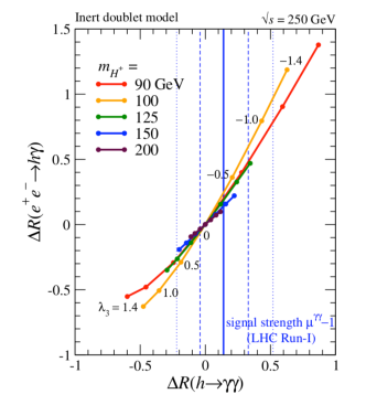
Figure 1: The relative deviations of the $e^{+}e^{-}\to h\gamma$ cross section and the $h\xrightarrow{}\gamma\gamma$ branching ratio with respect to the Standard Model values [2]

A usual method to measure $h\gamma\gamma$ and $h\gamma Z$ couplings is to use decay branching ratios of $h\to\gamma\gamma/\gamma Z$. It is, however, very challenging to measure the $h\to\gamma Z$ branching ratio even at the HL-LHC: only a 3$\sigma$ significance is expected. As a complementary method we study these couplings in a production process at the ILC, $e^{+}e^{-}\to h\gamma$ (see Figure 2).

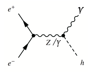
Figure 2: The Feynman diagram of $e^{+}e^{-}\to h\gamma$

In addition, the $h\gamma Z$ coupling appears in an s-channel photon exchange diagram for the leading single Higgs production process: $e^{+}e^{-}\to hZ$ in the effective field theory framework. It is hence necessary to know the contribution from this diagram. Furthermore, it turns out that the anomalous $h\gamma Z$, $h\gamma\gamma$, $hZZ$, and $hWW$ couplings come from a common set of a few dimension-6 operators, hence the measurement of the $h\gamma Z$ coupling using $e^{+}e^{-}\to h\gamma$ has a potential to provide one very useful constraint on those operators.

In section 2, we introduce our theoretical framework. In section 3, we describe our experimental method and simulation framework. In section 4, we present our event selection and analysis result. Section 5 gives our plan for further study.

2 Theoretical Framework

In this analysis, we use the effective Lagrangian shown in Equation 1 to include new physics contributions to the $e^{+}e^{-}\xrightarrow{}h\gamma$ cross section model-independently,

$${\cal{L}}_{h\gamma}={\cal{L}}_{\mathrm{SM}}+\frac{\zeta_{AZ}}{v}A_{\mu\nu}Z^{\mu\nu}h+\frac{\zeta_{A}}{2v}A_{\mu\nu}A^{\mu\nu}h,$$ (1)

where $\zeta_{AZ}$ and $\zeta_{A}$ terms represent respectively effective $h\gamma Z$ and $h\gamma\gamma$ couplings from new physics. $A_{\mu\nu}$, and $Z_{\mu\nu}$ are field strength tensors. $v$ is the vacuum expectation value. The first term is the Standard Model Lagrangian. The three terms contribute to $e^{+}e^{-}\to h\gamma$ process via the Feynman diagrams shown in Figure 3, where the first SM diagram represents several loop induced diagrams as shown in Figure 4.

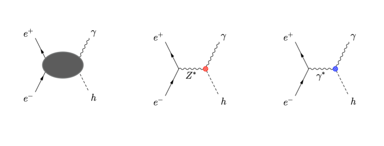
Figure 3: Diagrams arising from each of the three terms of Equation 1, respectively.

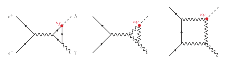
Figure 4: The loop induced Feynman diagrams in the Standard Model for $e^{+}e^{-}\to h\gamma$ [2]

The cross section normalized to SM can be written as Equation 2 and Equation 3 [4]. The SM cross sections at $\sqrt{s}$ = 250 GeV are calculated as shown in Table 1. The cross sections including effective $h\gamma Z/h\gamma\gamma$ couplings from new physics are calculated as in $P(e^{-},e^{+})=(+100\%,-100\%)$) , up to interference term.

$$\frac{\sigma_{\gamma H}}{\sigma_{SM}}=1-201\zeta_{A}-273\zeta_{AZ}$$ (2)

$$\frac{\sigma_{\gamma H}}{\sigma_{SM}}=1+492\zeta_{A}-311\zeta_{AZ}$$ (3)

Table 1: SM cross sections for different beam polarizations ($\sqrt{s}$ = 250 GeV )

$P_{e^{-}}$	$P_{e^{+}}$	$\sigma_{SM}$[fb]
-100$\%$	+100$\%$	0.35
+100$\%$	-100$\%$	0.016
-80$\%$	+30$\%$	0.20

3 Experimental Method and Simulation Framework

3.1 Experimental Method

In order to determine both $\zeta_{AZ}$ and $\zeta_{A}$, we need two measurements. There are two strategies:
1. to measure the cross sections of $e^{+}e^{-}\xrightarrow{}\gamma h$ for two different beam polarizations, and
2. to use the measurement of the $h\xrightarrow{}\gamma\gamma$ branching ratio at the LHC to constrain $\zeta_{A}$ and determine $\zeta_{AZ}$ by just measuring $e^{+}e^{-}\to h\gamma$ cross section for one single polarization.

3.2 Simulation framework

We use fully-simulated Monte-Carlo (MC) samples produced with the ILD detector model [3]. For event generation, we use Physsim [5] for signal, and Whizard [6] for background processes. For detector simulation, we use Mokka [7], which is based on Geant4 [8], and for event reconstruction, we use Marlin in iLCSoft [9], where particle flow analysis (PFA) is done with PandoraPFA [10] and flavor tagging is done with LCFI+ [11]. The analysis is carried out at $\sqrt{s}$=250 GeV, assuming an integrated luminosity of 2000 fb^-1.

4 Event Selection and Results

4.1 Event Selection

The signal channel studied in this paper is $e^{+}e^{-}\to h\gamma$, followed by $h\to b\bar{b}$. In the final states of the signal events, we expect one isolated monochromatic photon with an energy of $E_{\gamma}=\sqrt{s}/{2}\left(1-{\left(m_{h}/\sqrt{s}\right)}^{2}\right)=93$ GeV, where $m_{h}$ is the Higgs mass, and two $b$ jets with an invariant mass consistent with the Higgs mass. The enegy resolution of the electromagnetic calorimeter is given by $\sigma_{E}=0.16\times\sqrt{E}$ (GeV), where the photon energy $E$ is in units of GeV [3]. The energy resolution for the isolated photon is thus 1.5 GeV. The main background would be $e^{+}e^{-}\to\gamma q\bar{q}$, dominantly coming from $e^{+}e^{-}\to\gamma Z$.

As pre-selection, we start with identifying one isolated photon with an energy greater than 50 GeV. Sometimes, the reconstruction software PandoraPFA splits calorimetric clusters created by a single high energy photon into several objects. Such split clusters fall within a narrow cone ($\cos\theta_{cone}$=0.998, where $\cos\theta_{cone}$ is cone angle), and are considered as a single object in the following analysis.The particles other than the photon are clustered into two jets using the Durham algorithm [12].

In the final selection, the first cut requires two $b$ jets. Figure 5 shows the distribution normalized to unity of the larger $b$-likeliness value among the two jets for signal and background events. We require this larger $b$-likeliness to be greater than 0.77 to suppress the light flavor $\gamma q\bar{q}$ events. The cut value is optimized to maximize the signal significance defined as

$$\text{significance}=\frac{N_{S}}{\sqrt{N_{S}+N_{B}}},$$ (4)

where $N_{S}$ and $N_{B}$ are the numbers of signal and background events, respectively.

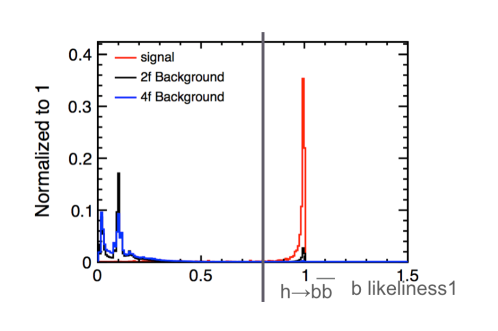
Figure 5: The distribution of $b$-likeliness for signal and background events with unit normalization

The second cut requires small enough missing energy. Figure 6 shows the missing energy distribution. We cut the missing energy at 35 GeV.

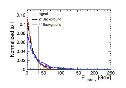
Figure 6: Normalized missing energy distribution for signal and background events

To finalize our event selection, we use a multivariate analysis method, the BDT algorithm as implemented in the TMVA package [13]. It is trained using five input variables: the 2-jet invariant mass, the energy of the isolated photon, its polar angle, the smaller angle between the photon and a jet, and the angle between the two jets. Figure 7 illustrates these input variables. Figure 8 shows the distributions of each input variable for signal and background events. The blue histograms are for signal events, and the red histograms are for background events. Our final cut requires the BDT output to be greater than 0.0126.

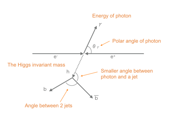
Figure 7: Input variables for TMVA

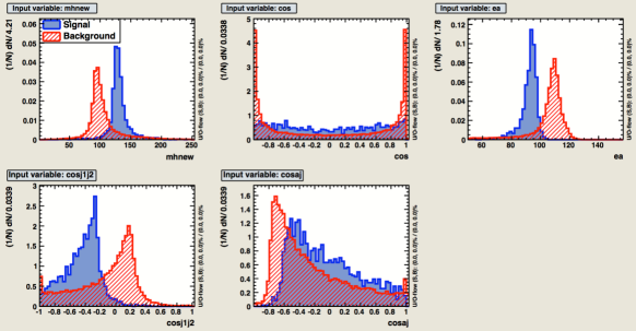
Figure 8: Distributions of TMVA input variables for signal and background events.

Figure 9 shows the distribution of $m(b\bar{b})$ after all the other cuts for the signal and background events normalized to an integrated luminosity of 2000 fb^-1 for the left-handed beam polarization. The remaining background events are dominated by 2-fermion processes.

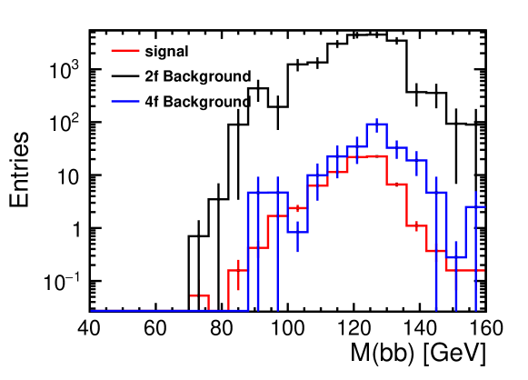
Figure 9: The distribution of $m(b\bar{b})$ after all the other cuts for the signal and background events normalized to 2000 fb^-1

4.2 Result

Table 2 gives the number of signal and background events, as well as the signal significance after each cut. The significance is defined by Equation 4. After all the cuts, the signal significance is expected to be 0.53$\sigma$, for the SM signal process $e^{+}e^{-}\to h\gamma$ followed by $h\to b\bar{b}$ decay. The 95 $\%$ confidence level upper limit for the cross section at $\sqrt{s}=250$ of $e^{+}e^{-}\to h\gamma$ is calculated using Equation 5 to be $\sigma_{h\gamma}^{CL95}<1.08$ fb, for 2000 fb^-1 GeV and left handed beam polarizations.

Table 2: The cut table

	Signal	background	Significance
Expected	237	3.14$\times 10^{8}$	0.01
Pre selection	222	6.54$\times 10^{7}$	0.02
$b_{tag}\geq$0.8	200	4.96$\times 10^{6}$	0.09
$E_{mis}\leq$35	182	4.30$\times 10^{6}$	0.09
$mvabdt\geq$ 0.0126	75	1.98$\times 10^{4}$	0.53

$$\sigma=\frac{1.64}{\text{ significance }}\sigma_{SM}$$ (5)

From this upper limit and Equation 2 and Table 1, we have

$$3.09>\frac{\sigma_{\gamma H}}{\sigma_{SM}}=1-201\zeta_{A}-273\zeta_{AZ}>0~{}(\mbox{assuming}~{}\zeta_{A}=0).$$ (6)

We can then set the bound on the parameter $\zeta_{AZ}$:

$$-0.0077>\zeta_{AZ}>0.0037.$$ (7)

5 Further Study

We are planning to improve the analysis by adding the $h\xrightarrow{}WW^{*}$ channel. The branching ratio of this channel is around 21$\%$ corresponding to about 50 event for 2000 fb^-1. The main background we expect in this channel would be $e^{+}e^{-}\to W^{+}W^{-}$ with a hard ISR photon, while in the $h\to b\bar{b}$ channel, the main background is $e^{+}e^{-}\to b\bar{b}$ with a hard ISR photon, which is significantly enhanced due to the radiative return to $Z$-pole. We would hence expect a higher signal to background ratio in the $h\to WW^{*}$ channel.

After $h\to WW^{*}$ channel is completed, the experimental bound on $\zeta_{AZ}$ will be translated into a bound on Dimension-6 operators.

References

- [1] T. Behnke et al., “The International Linear Collider Technical Design Report - Volume 1: Executive Summary,” arXiv:1306.6327 [physics.acc-ph].
- [2] S. Kanemura, K. Mawatari and K. Sakurai, “Single Higgs production in association with a photon at electron-positron colliders in extended Higgs models,” arXiv:1808.10268 [hep-ph].
- [3] T. Behnke et al., “The International Linear Collider Technical Design Report - Volume 4: Detectors,” arXiv:1306.6329 [physics.ins-det].
- [4] K. Fujii, J. Tian and H. Yokoya, “Diphoton resonance at the ILC,” Phys. Rev. D 94, no. 9, 095015 (2016) doi:10.1103/PhysRevD.94.095015 [arXiv:1607.04187 [hep-ph]].
- [5] Physsim home page http://www-jlc.kek.jp/subg/offl/physsim/
- [6] W. Kilian, T. Ohl and J. Reuter, “WHIZARD: Simulating Multi-Particle Processes at LHC and ILC,” Eur. Phys. J. C 71, 1742 (2011) doi:10.1140/epjc/s10052-011-1742-y [arXiv:0708.4233 [hep-ph]].
- [7] Mokka Home page, http://ilcsoft.desy.de/portal/software_packages/mokka/
- [8] S. Agostinelli et al. (GEANT4 Collaboration), “Geant4—a simulation toolkit,” Nucl.Instrum. Methods Phys. Res., Sect. A 506, 250 (2003).
- [9] F. Gaede, J. Engels, “Marlin et al - A Software Framework for ILC detector R&D,”EUDET-Report-2007-11.
- [10] M. A. Thomson, “Particle Flow Calorimetry and the PandoraPFA Algorithm,” Nucl. Instrum. Meth. A 611, 25 (2009) doi:10.1016/j.nima.2009.09.009 [arXiv:0907.3577 [physics.ins-det]].
- [11] T. Suehara and T. Tanabe, “LCFIPlus: A Framework for Jet Analysis in Linear Collider Studies,” Nucl. Instrum. Meth. A 808, 109 (2016) doi:10.1016/j.nima.2015.11.054 [arXiv:1506.08371 [physics.ins-det]].
- [12] S. Catani, Y. L. Dokshitzer, M. Olsson, G. Turnock and B. R. Webber, “New clustering algorithm for multi - jet cross-sections in e+ e- annihilation,” Phys. Lett. B 269, 432 (1991). doi:10.1016/0370-2693(91)90196-W
- [13] A. Hoecker, et al. “TMVA-Toolkit for multivariate data analysis,” arXiv preprint physics/0703039 (2007).