Characterizing the Nonlinearity of Power System Generator Models

Abstract

Power system dynamics are naturally nonlinear. The nonlinearity stems from power flows, generator dynamics, and electromagnetic transients. Characterizing the nonlinearity of the dynamical power system model is useful for designing superior estimation and control methods, providing better situational awareness and system stability. In this paper, we consider the synchronous generator model with a phasor measurement unit (PMU) that is installed at the terminal bus of the generator. The corresponding nonlinear process-measurement model is shown to be locally Lipschitz, i.e., the dynamics are limited in how fast they can evolve in an arbitrary compact region of the state-space. We then investigate different methods to compute Lipschitz constants for this model, which is vital for performing dynamic state estimation (DSE) or state-feedback control using Lyapunov theory. In particular, we compare a derived analytical bound with numerical methods based on low discrepancy sampling algorithms. Applications of the computed bounds to dynamic state estimation are showcased. The paper is concluded with numerical tests.

I Introduction

Single- and multi-machine power system models have been thoroughly developed and explored in the literature of power systems [1, 2]. These models describe the electromagnetic transients of interconnected generators in transmission networks, ranging from the simple second-order swing equations to tenth or higher-order, nonlinear differential algebraic equation representations. By considering that phasor measurement units (PMUs) are installed at the terminal buses of selected generators, a nonlinear, dynamical power system model can be generally described as follows

$${}\dot{\bm{x}}(t)=\tilde{\bm{f}}(\bm{x},\bm{u}),\quad\;\;\bm{y}(t)=\tilde{\bm{h}}(\bm{x},\bm{u}),$$ (1)

where $\bm{x}(t)$ represents the dynamic state vector, $\bm{u}(t)$ depicts the known or unknown input vector, and $\bm{y}(t)$ models the output measurements from PMUs [3].

Dynamic modeling of power systems is important because it can guide the development of open- or closed-loop control algorithms. This is in addition to dynamic state estimation (DSE) routines [4, 5, 6, 7, 8]—under the presence of unknown inputs, disturbances, faults, and noise. The majority of state-feedback control algorithms that utilize low- or high-order linearized power system models, or low-order nonlinear models, such as proportional-integral control, linear quadratic regulator, $\mathcal{H}_{2}$, $\mathcal{H}_{\infty}$, mixed $\mathcal{H}_{2}$/$\mathcal{H}_{\infty}$, and model predictive control have been applied to power systems. Our recent work on robust control in power systems succinctly lists the main control algorithms used in the above context [9].

Although advanced static state estimation technique for power systems are still being developed, for example, to minimize the impact of cyber attacks [10], DSE is considered to be superior due to its capability for performing state estimation in almost real time. Particularly for DSE and state observers in power systems, many studies have used power system models with different levels of details, with overwhelming focus on Kalman filters and its different variants; see our recent paper [3] and the references therein for a comparison of DSE approaches in power systems. Surprisingly, systems-theoretic observer designs are less common in the literature of power system DSE—especially when compared with feedback control algorithms.

With that in mind, we are interested in utilizing observer-based approach to perform DSE while considering the nonlinear dynamics model of power systems. To do so, first we need to classify the nonlinearities in power system models (that is, $\tilde{\bm{f}}(\cdot)$ and $\tilde{\bm{h}}(\cdot)$ in (1)) as they can be classified into an abundance of function sets such as Lipschitz continuous, one-sided Lipschitz, quadratic inner-boundedness, or bounded Jacobian [11, 12, 3, 13]. Here, we put our interest on Lipschitz nonlinearity because of its simplicity. It is worth noticing that the majority of Lipschitz-based observer for nonlinear systems cannot cope with relatively large (or conservative) Lipschitz constants. Because of this reason, in this paper we (a) investigate different methods (analytical and numerical) to compute/approximate Lipschitz constants for a synchronous generator model, (b) compare the Lipschitz constants obtained from the two methods, and (c) check their applicability for performing DSE on single generator using a vintage Lipschitz-based observer proposed in[12], which is akin to the Luenberger observer.

The presented research here is motivated by the work of Siljak et al. [14] on robust decentralized control of power systems. By proving that the nonlinearity in the considered model is quadratically bounded, decentralized control framework considering nonlinear model of power systems are developed in [14]. The ideas from [14] are then extended by Lian et al. [15] with applications to enhancement of damping ratios of the inter-area oscillation through decentralized robust control [15]. As for DSE methods, our recent work [3] assumes that a higher-order, multi-machine power system model is one-sided Lipschitz and quadratically inner-bounded. This assumption is then followed by designing a DSE method for uncertain power systems. The study by Jin et al. [13] considers the problem of designing a DSE method for a general class of nonlinear Lipschitz dynamic systems, with applications to interconnected power systems using the second-order swing equations and a linear measurement model. The authors show that the proposed DSE method is less conservative than its counterparts, making it attractive for large-scale systems.

In short, this paper aims to investigate different methods to obtain the Lipschitz constants which can be used to perform DSE on a single generator using Lipchitz-based observer. The paper contributions and organization are summarized as follows. First, we reproduce the fourth-order generator model with PMU measurements as outputs (Section II). This model has been used in DSE studies and shown to be able to estimate the nonlinear behavior of the generator [6]. Second, we propose an analytical method to compute Lipschitz constants for the process and PMU measurement models, which depends on the bounds of the state and input vectors (Section III). Third, we propose a simple sampling-based numerical algorithm that, in theory, could generate less conservative Lipschitz (Section IV). Fourth, we briefly present a Lipschitz-based observer that is crucial for performing DSE (Section V). Finally, in addition to comparing the results of obtaining Lipschitz constants using the two aforementioned methods, we present an application of the proposed theoretical/computational bounds to DSE of generator states given PMU measurements (Section VI).

II Generator Dynamic Model

It is usually difficult to directly measure the internal states of a synchronous generator. By contrast, with PMU installed at the terminal bus of the generator, the voltage and current phasors can be easily measured and can then be used to estimate the internal states of the generator [6, 8]. Here, we focus on modeling and understanding the nonlinearities of PMU-connected single synchronous generator. For generator $i$, the fast sub-transient dynamics and saturation effects are ignored and the generator model is described by the fourth-order differential equations in local $\mathrm{d}$-$\mathrm{q}$ reference frame [2]

$$\dot{\delta_{i}}=\omega_{i}-\omega_{0}$$ (2a)

$$\dot{\omega}_{i}=\frac{\omega_{0}}{2H_{i}}\Big{(}T_{\textrm{m}i}-T_{\textrm{e}i}-\frac{K_{\textrm{D}i}}{\omega_{0}}(\omega_{i}-\omega_{0})\Big{)}$$ (2b)

$$\dot{e}^{\prime}_{\textrm{q}i}=\frac{1}{T^{\prime}_{\textrm{d0}i}}\Big{(}E_{\textrm{fd}i}-e^{\prime}_{\textrm{q}i}-(x_{\textrm{d}i}-x^{\prime}_{\textrm{d}i})\,i_{\textrm{d}i}\Big{)}$$ (2c)

$$\dot{e}^{\prime}_{\textrm{d}i}=\frac{1}{T^{\prime}_{\textrm{q0}i}}\Big{(}-e^{\prime}_{\textrm{d}i}+(x_{\textrm{q}i}-x^{\prime}_{\textrm{q}i})\,i_{\textrm{q}i}\Big{)},$$ (2d)

where $\delta_{i}(t):=\delta_{i}$ is the rotor angle, $\omega_{i}(t):=\omega$ is the rotor speed in rad/s, and $e^{\prime}_{\mathrm{q}i}(t):=e^{\prime}_{\mathrm{q}i}$ and $e^{\prime}_{\mathrm{d}i}(t):=e^{\prime}_{\mathrm{d}i}$ are the transient voltage along $\mathrm{q}$ and $\mathrm{d}$ axes; $i_{\mathrm{q}i}(t):=i_{\mathrm{q}i}$ and $i_{\mathrm{d}i}(t):=i_{\mathrm{d}i}$ are stator currents at $\mathrm{q}$ and $\mathrm{d}$ axes; $T_{\mathrm{m}i}(t):=T_{\mathrm{m}i}$ is the mechanical torque, $T_{\mathrm{e}i}(t):=T_{\mathrm{e}i}$ is the electric air-gap torque, and $E_{\mathrm{fd}i}(t):=E_{\mathrm{fd}i}$ is the internal field voltage; $\omega_{0}$ is the rated value of angular frequency, $H_{i}$ is the inertia constant, and $K_{\mathrm{D}i}$ is the damping factor; $T^{\prime}_{\mathrm{q0}i}$ and $T^{\prime}_{\mathrm{d0}i}$ are the open-circuit time constants for $\mathrm{q}$ and $\mathrm{d}$ axes; $x_{\mathrm{q}i}$ and $x_{\mathrm{d}i}$ are the synchronous reactance and $x^{\prime}_{\mathrm{q}i}$ and $x^{\prime}_{\mathrm{d}i}$ are the transient reactance respectively at the $\mathrm{q}$ and $\mathrm{d}$ axes. We assume that a PMU is installed at the terminal bus of generator $i$. The mechanical torque $T_{\mathrm{m}i}$ and internal field voltage $E_{\mathrm{fd}i}$ are considered as inputs which can be measured/estimated [6]. Additionally, we take the current phasor $I_{ti}=i_{\mathrm{R}i}+i_{\mathrm{I}i}$ measured by PMU as inputs which can help decouple generator $i$ from the rest of the network [6]. The voltage phasor $E_{ti}=e_{\mathrm{R}i}+e_{\mathrm{I}i}$ can also be measured by PMU and is considered as output. The dynamic model (2d) can be rewritten in a general state-space form (1) where the state, input, and output vectors are specified as

$$\bm{x}=\begin{bmatrix}x_{1}\quad x_{2}\quad x_{3}\quad x_{4}\end{bmatrix}^{\top}=\begin{bmatrix}\delta_{i}\quad\omega_{i}\quad e^{\prime}_{\mathrm{q}i}\quad e^{\prime}_{\mathrm{d}i}\end{bmatrix}^{\top}$$ (3a)

$$\bm{u}=\begin{bmatrix}u_{1}\quad u_{2}\quad u_{3}\quad u_{4}\end{bmatrix}^{\top}=\begin{bmatrix}T_{\mathrm{m}i}\quad E_{\mathrm{fd}i}\quad i_{\mathrm{R}i}\quad i_{\mathrm{I}i}\end{bmatrix}^{\top}$$ (3b)

$$\bm{y}=\begin{bmatrix}y_{1}\quad y_{2}\end{bmatrix}^{\top}=\begin{bmatrix}e_{\mathrm{R}i}\quad e_{\mathrm{I}i}\end{bmatrix}^{\top}.$$ (3c)

The $i_{\textrm{q}i}$, $i_{\textrm{d}i}$, and $T_{\textrm{e}i}$ in (2d) are functions of $\bm{x}$ and $\bm{u}$ as follows

$$i_{\textrm{q}i}=i_{\textrm{I}i}\sin\delta_{i}+i_{\textrm{R}i}\cos\delta_{i}=u_{4}\sin x_{1}+u_{3}\cos x_{1}$$

$$i_{\textrm{d}i}=i_{\textrm{R}i}\sin\delta_{i}-i_{\textrm{I}i}\cos\delta_{i}=u_{3}\sin x_{1}-u_{4}\cos x_{1}$$

$$e_{\textrm{q}i}=e^{\prime}_{\textrm{q}i}-\frac{S_{\textrm{B}}}{S_{\textrm{N}i}}x^{\prime}_{\textrm{d}i}i_{\textrm{d}i}=x_{3}-\frac{S_{\textrm{B}}}{S_{\textrm{N}i}}x^{\prime}_{\textrm{d}i}i_{\textrm{d}i}$$ (4)

$$e_{\textrm{d}i}=e^{\prime}_{\textrm{d}i}+\frac{S_{\textrm{B}}}{S_{\textrm{N}i}}x^{\prime}_{\textrm{q}i}i_{\textrm{q}i}=x_{4}+\frac{S_{\textrm{B}}}{S_{\textrm{N}i}}x^{\prime}_{\textrm{q}i}i_{\textrm{q}i}$$

$$P_{\textrm{e}i}=e_{\textrm{q}i}i_{\textrm{q}i}+e_{\textrm{d}i}i_{\textrm{d}i}\,\quad T_{\textrm{e}i}=\frac{S_{\textrm{B}}}{S_{\textrm{N}i}}P_{\textrm{e}i},$$

where $e_{\mathrm{q}i}$ and $e_{\mathrm{d}i}$ are the terminal voltage at $\mathrm{q}$ and $\mathrm{d}$ axes, and $S_{\mathrm{B}}$ and $S_{\mathrm{N}i}$ are the system base MVA and the base MVA for generator $i$, respectively. The PMU outputs $e_{\textrm{R}i}$ and $e_{\textrm{I}i}$ can be written as functions of $\bm{x}$ and $\bm{u}$ as follows

$$e_{\textrm{R}i}=e_{\textrm{d}i}\sin\delta_{i}+e_{\textrm{q}i}\cos\delta_{i},\;e_{\textrm{I}i}=e_{\textrm{q}i}\sin\delta_{i}-e_{\textrm{d}i}\cos\delta_{i}.$$ (5)

By substituting (3) and (4) to (2d) and (5), the generator’s dynamics can be modeled into the following form

$$\dot{\bm{x}}=\bm{A}\bm{x}+\bm{f}(\bm{x},\bm{u})+\bm{B_{\mathrm{u}}}\bm{u}$$ (6a)

$$\bm{y}=\bm{h}(\bm{x},\bm{u})+\bm{D_{\mathrm{u}}}\bm{u},$$ (6b)

where $\bm{A},\bm{B}_{u},$ and $\bm{D}_{u}$ are the state-space matrices given in Appendix A, and the functions $\bm{f}(\cdot)$ and $\bm{h}(\cdot)$ are given as

$$f_{1}(\bm{x},\bm{u}) =-\alpha_{1}$$ (7a)

$$f_{2}(\bm{x},\bm{u}) =\alpha_{3}x_{4}u_{4}\cos x_{1}-\alpha_{3}x_{3}u_{4}\sin x_{1}-\alpha_{3}x_{4}u_{3}\sin x_{1}$$

$$\,\quad-\alpha_{3}x_{3}u_{3}\cos x_{1}+\alpha_{4}u_{3}u_{4}\cos 2x_{1}$$

$$\,\quad+\tfrac{1}{2}\alpha_{4}\left(u_{4}^{2}-u_{3}^{2}\right)\sin 2x_{1}+\alpha_{6}$$ (7b)

$$f_{3}(\bm{x},\bm{u}) =\alpha_{8}u_{4}\cos x_{1}-\alpha_{8}u_{3}\sin x_{1}$$ (7c)

$$f_{4}(\bm{x},\bm{u}) =\alpha_{10}u_{3}\cos x_{1}+\alpha_{10}u_{4}\sin x_{1}$$ (7d)

$$h_{1}(\bm{x},\bm{u}) =x_{3}\cos x_{1}+x_{4}\sin x_{1}+\beta_{1}u_{3}\sin 2x_{1}$$

$$\quad+\beta_{1}u_{4}\cos 2x_{1}$$ (7e)

$$h_{2}(\bm{x},\bm{u}) =x_{3}\sin x_{1}-x_{4}\cos x_{1}-\beta_{1}u_{3}\cos 2x_{1}$$

$$\quad-\beta_{1}u_{4}\sin 2x_{1},$$ (7f)

where constants $\alpha_{1,2,\cdot,10}$ and $\beta_{1,2}$ are described in Appendix A. The next section provides analytical methods to compute the Lipschitz constants for $\bm{f}(\cdot)$ and $\bm{h}(\cdot)$.

III The Computation of Lipschitz Constant

It is evident from (6b) that the generator dynamic model is highly nonlinear. As mentioned earlier, it is important to understand the behavior of the nonlinearities involved in $\bm{f}(\cdot)$ and $\bm{h}(\cdot)$. By assuming that the state vector $\bm{x}$ and input vector $\bm{u}$ belong to certain compact sets, as stated in Assumption 1, the characteristics of the nonlinearity can then be studied—either analytically or numerically.

Assumption 1.

The state vector $\bm{x}$ and input vector $\bm{u}$ in (6b) are bounded such that $\bm{x}\in\mathbfcal{X}$ and $\bm{x}\in\mathbfcal{U}$ where

$$\mathbfcal{X} :=\left[\stackunder[1.2pt]{$x$}{\rule{3.44444pt}{0.32289pt}}_{1},\bar{x}_{1}\right]\times\left[\stackunder[1.2pt]{$x$}{\rule{3.44444pt}{0.32289pt}}_{2},\bar{x}_{2}\right]\times\left[\stackunder[1.2pt]{$x$}{\rule{3.44444pt}{0.32289pt}}_{3},\bar{x}_{3}\right]\times\left[\stackunder[1.2pt]{$x$}{\rule{3.44444pt}{0.32289pt}}_{4},\bar{x}_{4}\right]$$ (8a)

$$\mathbfcal{U} :=\left[\stackunder[1.2pt]{$u$}{\rule{3.44444pt}{0.32289pt}}_{1},\bar{u}_{1}\right]\times\left[\stackunder[1.2pt]{$u$}{\rule{3.44444pt}{0.32289pt}}_{2},\bar{u}_{2}\right]\times\left[\stackunder[1.2pt]{$u$}{\rule{3.44444pt}{0.32289pt}}_{3},\bar{u}_{3}\right]\times\left[\stackunder[1.2pt]{$u$}{\rule{3.44444pt}{0.32289pt}}_{4},\bar{u}_{4}\right].$$ (8b)

Realize that the above assumption is practical and holds for most power systems models as physical quantities such as angles and frequencies are naturally bounded. Since $\bm{f}(\cdot)$ and $\bm{h}(\cdot)$ are bounded and continuously differentiable, both are locally Lispchitz continuous. The following introduces the definition of Lipschitz continuity.

Definition 1.

Let $\bm{g}:\mathbb{R}^{m}\rightarrow\mathbb{R}^{n}$ be a function. Then, $\bm{g}$ is Lipschitz continuous in $\mathbfcal{B}\subseteq\mathbb{R}^{m}$ if there exists a constant $\gamma\geq 0$ such that for all $\bm{x},\hat{\bm{x}}\in\mathbfcal{B}$

$$\left\lVert\bm{g}(\bm{x})-\bm{g}(\hat{\bm{x}})\right\rVert_{2}\leq\gamma\left\lVert\bm{x}-\hat{\bm{x}}\right\rVert_{2}.$$ (9)

The best (ideal) Lipschitz constant is the smallest $\gamma$ satisfying (9). Although desirable, finding such $\gamma$ can be challenging. To that end, we use the following lemma to compute a Lipschitz constant $\gamma$ which, albeit not giving the smallest constant, can still be useful for our purpose—see Section VI.

Lemma 1.

Let $\bm{g}:\mathbb{R}^{m}\rightarrow\mathbb{R}^{n}$ and $\bm{x},\hat{\bm{x}}\in\mathbfcal{B}$ where $\mathbfcal{B}\subseteq\mathbb{R}^{m}$. If there exists $\gamma_{i}\geq 0$ such that

$$\left\lvert g_{i}(\bm{x})-g_{i}(\hat{\bm{x}})\right\rvert\leq\gamma_{i}\left\lVert\bm{x}-\hat{\bm{x}}\right\rVert_{2},$$ (10)

for all $i=1,\ldots,n$, then $\bm{g}$ is Lipschitz continuous in $\mathbfcal{B}$ with Lipschitz constant $\gamma=\sqrt{\sum_{i=1}^{n}\gamma^{2}_{i}}$.

The proof of Lemma 1 is omitted here for brevity. By virtue of this lemma, the following result presents analytical formulations to compute the corresponding Lipschitz constants for the two functions.

Theorem 1.

Consider $\bm{f}:\mathbb{R}^{4}\times\mathbb{R}^{4}\rightarrow\mathbb{R}^{4}$ and $\bm{h}:\mathbb{R}^{4}\times\mathbb{R}^{4}\rightarrow\mathbb{R}^{2}$ from (6b). Then, for any $\bm{x},\hat{\bm{x}}\in\mathbfcal{X}$ and $\bm{u}\in\mathbfcal{U}$, we have

$$\left\lVert\bm{f}(\bm{x},\bm{u})-\bm{f}(\hat{\bm{x}},\bm{u})\right\rVert_{2}\leq\gamma_{f}\left\lVert\bm{x}-\hat{\bm{x}}\right\rVert_{2}$$ (11a)

$$\left\lVert\bm{h}(\bm{x},\bm{u})-\bm{h}(\hat{\bm{x}},\bm{u})\right\rVert_{2}\leq\gamma_{h}\left\lVert\bm{x}-\hat{\bm{x}}\right\rVert_{2},$$ (11b)

where constants $\gamma_{f}$ and $\gamma_{h}$ are given as

$$\gamma_{f} =\sqrt{\tilde{\gamma}_{f}^{2}+\left(\left\lvert\alpha_{8}\right\rvert^{2}+\left\lvert\alpha_{10}\right\rvert^{2}\right)\left(\kappa_{\mathrm{u}3}+\kappa_{\mathrm{u}4}\right)^{2}}$$ (12a)

$$\gamma_{h} =\sqrt{2}\left(\kappa_{\mathrm{x}3}+\kappa_{\mathrm{x}4}+2\left\lvert\beta_{1}\right\rvert\left(\kappa_{\mathrm{u}3}+\kappa_{\mathrm{u}4}\right)+\sqrt{2}\right),$$ (12b)

and $$\tilde{\gamma}_{f}$$ in (12a) is specified as

$$\tilde{\gamma}_{f} =\left\lvert\alpha_{3}\right\rvert\left(\left(\kappa_{\mathrm{u}3}+\kappa_{\mathrm{u}4}\right)\left(1+\kappa_{\mathrm{x}3}+\kappa_{\mathrm{x}4}\right)+2\kappa_{\mathrm{u}3}\kappa_{\mathrm{u}4}\right)$$

$$\quad+\left\lvert\alpha_{4}\right\rvert\left(\kappa_{\mathrm{u}3}\left(1+\kappa_{\mathrm{u}3}\right)+\kappa_{\mathrm{u}4}\left(1+\kappa_{\mathrm{u}4}\right)\right),$$ (12c)

with $\kappa_{\mathrm{x}i}:=\mathrm{max}\left(\left\lvert\stackunder[1.2pt]{$x$}{\rule{3.44444pt}{0.32289pt}}_{i}\right\rvert,\left\lvert\bar{x}_{i}\right\rvert\right)$ and $\kappa_{\mathrm{u}j}:=\mathrm{max}\left(\left\lvert\stackunder[1.2pt]{$u$}{\rule{3.44444pt}{0.32289pt}}_{j}\right\rvert,\left\lvert\bar{u}_{j}\right\rvert\right)$.

Proof.

Let $\bm{x},\hat{\bm{x}}\in\mathbfcal{X}$ and $\bm{u}\in\mathbfcal{U}$. First, for $f_{1}(\cdot)$ given in (7a), we have

$$\left\lvert f_{1}\left(\bm{x},\bm{u}\right)-f_{1}\left(\hat{\bm{x}},\bm{u}\right)\right\rvert=\left\lvert-\alpha_{1}-(-\alpha_{1})\right\rvert=0.$$ (13a)

Next, for $$f_{2}(\cdot)$$ given in (7b), we obtain

$$| f_{2}\left(\bm{x},\bm{u}\right)-f_{2}\left(\hat{\bm{x}},\bm{u}\right)|\leq\left\lvert\alpha_{3}u_{4}\right\rvert\left(\left\lvert x_{3}\sin x_{1}-\hat{x}_{3}\sin\hat{x}_{1}\right\rvert\right.$$

$$\;\left.+\left\lvert x_{4}\cos x_{1}-\hat{x}_{4}\cos\hat{x}_{1}\right\rvert\right)+\left\lvert\alpha_{3}u_{3}\right\rvert\left(\left\lvert x_{3}\cos x_{1}-\hat{x}_{3}\cos\hat{x}_{1}\right\rvert\right.$$

$$\;\left.+\left\lvert x_{4}\sin x_{1}-\hat{x}_{4}\sin\hat{x}_{1}\right\rvert\right)+\left\lvert\alpha_{3}u_{3}u_{4}\right\rvert\left\lvert\cos 2x_{1}-\cos 2\hat{x}_{1}\right\rvert$$

$$\;+\tfrac{1}{2}\left\lvert\alpha_{4}\left(u_{4}^{2}-u_{3}^{2}\right)\right\rvert\left\lvert\sin 2x_{1}-\sin 2\hat{x}_{1}\right\rvert.$$

Since $$\left\lvert\sin 2x_{1}-\sin 2\hat{x}_{1}\right\rvert\leq 2\left\lvert x_{1}-\hat{x}_{1}\right\rvert \left\lvert\cos 2x_{1}-\cos 2\hat{x}_{1}\right\rvert\leq 2\left\lvert x_{1}-\hat{x}_{1}\right\rvert \left\lvert x_{i}\sin x_{1}-\hat{x}_{i}\sin\hat{x}_{1}\right\rvert\leq\kappa_{x,i}\left\lvert x_{1}-\hat{x}_{1}\right\rvert+\left\lvert x_{i}-\hat{x}_{i}\right\rvert \left\lvert x_{i}\cos x_{1}-\hat{x}_{i}\cos\hat{x}_{1}\right\rvert\leq\kappa_{x,i}\left\lvert x_{1}-\hat{x}_{1}\right\rvert+\left\lvert x_{i}-\hat{x}_{i}\right\rvert i=3,4$$, , , and for , then we ultimately get

$$|f_{2}\left(\bm{x},\bm{u}\right) -f_{2}\left(\hat{\bm{x}},\bm{u}\right)|\leq\tilde{\gamma}_{f}\left\lVert\bm{x}-\hat{\bm{x}}\right\rVert_{2},$$ (13b)

where $$\tilde{\gamma}_{f} f_{3}(\cdot)$$ is given in (12c). For given in (7c), we have

$$|f_{3}\left(\bm{x},\bm{u}\right)-f_{3}\left(\hat{\bm{x}},\bm{u}\right)| \leq\left\lvert\alpha_{8}\right\rvert\left\lvert u_{3}\right\rvert\left\lvert\sin x_{1}-\sin\hat{x}_{1}\right\rvert$$

$$\quad+\left\lvert\alpha_{8}\right\rvert\left\lvert u_{4}\right\rvert\left\lvert\cos x_{1}-\cos\hat{x}_{1}\right\rvert$$

$$\leq\left\lvert\alpha_{8}\right\rvert\left(\kappa_{\mathrm{u}3}+\kappa_{\mathrm{u}4}\right)\left\lVert\bm{x}-\hat{\bm{x}}\right\rVert_{2}.$$ (13c)

Last, for $$f_{4}(\cdot)$$ given in (7d), we obtain

$$|f_{4}\left(\bm{x},\bm{u}\right)-f_{4}\left(\hat{\bm{x}},\bm{u}\right)| \leq\left\lvert\alpha_{10}\right\rvert\left\lvert u_{4}\right\rvert\left\lvert\sin x_{1}-\sin\hat{x}_{1}\right\rvert$$

$$\quad+\left\lvert\alpha_{10}\right\rvert\left\lvert u_{3}\right\rvert\left\lvert\cos x_{1}-\cos\hat{x}_{1}\right\rvert$$

$$\leq\left\lvert\alpha_{10}\right\rvert\left(\kappa_{\mathrm{u}3}+\kappa_{\mathrm{u}4}\right)\left\lVert\bm{x}-\hat{\bm{x}}\right\rVert_{2}.$$ (13d)

Applying Lemma 1 to equations (13) yields (11a) with $\gamma_{f}$ is equals to (12a). Likewise, for for $h_{1}(\cdot)$ given in (7e), we have

$$|h_{1}\left(\bm{x},\bm{u}\right)-h_{1}\left(\hat{\bm{x}},\bm{u}\right)|\leq\left\lvert x_{4}\sin x_{1}-\hat{x}_{4}\sin\hat{x}_{1}\right\rvert$$

$$\quad+\left\lvert x_{3}\cos x_{1}-\hat{x}_{3}\cos\hat{x}_{1}\right\rvert+\left\lvert\beta_{1}\right\rvert\left\lvert u_{3}\right\rvert\left\lvert\sin 2x_{1}-\sin 2\hat{x}_{1}\right\rvert$$

$$\quad+\left\lvert\beta_{1}\right\rvert\left\lvert u_{4}\right\rvert\left\lvert\cos 2x_{1}-\cos 2\hat{x}_{1}\right\rvert$$

$$\leq\left(\vphantom{\sqrt{2}}\kappa_{\mathrm{x}3}+\kappa_{\mathrm{x}4}+2\left\lvert\beta_{1}\right\rvert\left(\kappa_{\mathrm{u}3}+\kappa_{\mathrm{u}4}\right)\right.\left.+\sqrt{2}\right)\left\lVert\bm{x}-\hat{\bm{x}}\right\rVert_{2}.$$ (14a)

Finally, for $$h_{2}(\cdot)$$ given in (7f), we obtain

$$|h_{2}\left(\bm{x},\bm{u}\right)-h_{2}\left(\hat{\bm{x}},\bm{u}\right)|\leq\left\lvert x_{3}\sin x_{1}-\hat{x}_{3}\sin\hat{x}_{1}\right\rvert$$

$$\quad+\left\lvert x_{4}\cos x_{1}-\hat{x}_{4}\cos\hat{x}_{1}\right\rvert+\left\lvert\beta_{1}\right\rvert\left\lvert u_{3}\right\rvert\left\lvert\cos 2x_{1}-\cos 2\hat{x}_{1}\right\rvert$$

$$\quad+\left\lvert\beta_{1}\right\rvert\left\lvert u_{4}\right\rvert\left\lvert\sin 2x_{1}-\sin 2\hat{x}_{1}\right\rvert$$

$$\leq\left(\vphantom{\sqrt{2}}\kappa_{\mathrm{x}3}+\kappa_{\mathrm{x}4}+2\left\lvert\beta_{1}\right\rvert\left(\kappa_{\mathrm{u}3}+\kappa_{\mathrm{u}4}\right)\right.\left.+\sqrt{2}\right)\left\lVert\bm{x}-\hat{\bm{x}}\right\rVert_{2}.$$ (14b)

Applying Lemma 1 to equations (14) yields (11b) with $\gamma_{h}$ is equals to (12b), thus completing the proof. ∎

That is, given the operational range of $\bm{x}$ and $\bm{u}$, the corresponding Lipschitz constants $\gamma_{f}$ and $\gamma_{h}$ for $\bm{f}(\cdot)$ and $\bm{h}(\cdot)$ can be computed. Notice that these constants are dependent on $\mathbfcal{X}$ and $\mathbfcal{U}$. For power systems having a large operational range, the resulting constants can be conservative, which is undesirable due to limitations on most Lipschitz-based observers that are only suitable for nonlinear systems with small Lipschitz constants [11]. With that in mind, the numerical tests investigate this presumed conservatism. To overcome this potential limitation, in the next section we also propose a simple numerical algorithm to approximate Lipschitz constants, thereby yielding smaller values of $\gamma_{f}$ and $\gamma_{h}$.

IV Numerical Algorithms to Compute $\gamma_{f}$ and $\gamma_{h}$

Here we propose numerical algorithms to approximate Lipschitz constant $\gamma_{f}$ and $\gamma_{h}$. The algorithm presented here essentially works by evaluating sample points randomly generated in the domain of interest. This technique is usually referred to as a Monte Carlo method[16]. While pure Monte Carlo methods use random sampling technique, Quasi-Monte Carlo methods use a pseudo-random technique that utilize low-discrepancy sequences (LDS). LDS are essentially sequence of points that are distributed almost equally in the domain. The concept of discrepancy itself can be explained as follows.

Let $\mathbfcal{Z}\subset\mathbb{R}^{n}$ be the domain of interest and suppose that there are $s$ number of points in that domain so that they can be written as a sequence of points $\mathcal{S}(\bm{z},s):=\left\{\bm{z}_{i}\right\}^{s}_{i=1}$ for each $\bm{z}_{i}\in\mathbfcal{Z}$. Then, define an interval $\bm{J}\subset\mathbfcal{Z}$ where $\bm{J}:=\prod^{n}_{j=1}[\stackunder[1.2pt]{$z$}{\rule{3.44444pt}{0.32289pt}}_{j},\bar{z}_{j})$ such that $\stackunder[1.2pt]{$z$}{\rule{3.44444pt}{0.32289pt}}_{j}\leq z_{j}<\bar{z}_{j}$ for all $j=1,\ldots,n$. That is, $\bm{J}$ defines a $n$-dimensional hypercube in $\mathbfcal{Z}$ specified by lower and upper bounds of each component for each point $\bm{z}_{i}$ in the sequence $\mathcal{S}(\bm{z},s)$. Consider that $\mathcal{P}(\bm{J})$ denotes the number of points lying in $\bm{J}$ and $\mathcal{V}(\bm{J})$ denotes the volume (or $n$-dimensional Lebesgue measure) of $\bm{J}$, then discrepancy $\mathit{D}(\cdot)$ is a measure formally defined as [16]

$$\mathit{D}(\bm{J},\mathcal{S}):=\left\lvert\frac{\mathcal{P}(\bm{J})}{s}-\mathcal{V}(\bm{J})\right\rvert,$$

The quantity $\mathit{D}(\cdot)$ quantifies the difference between the density of $\bm{J}$ (the proportion of points in $\bm{J}$ compared to the all points in the sequence) and the volume of $\bm{J}$ (the proportion of the size of $\bm{J}$ compared to the size of $\mathbfcal{Z}$). If there is a collection of $m$ intervals called $\mathbfcal{J}$ such that $\bm{J}_{k}\in\mathbfcal{J}$ for $1\leq k\leq m$, then the star-discrepancy can be regarded as the worst-case discrepancy [16], i.e., $\mathit{D}^{*}(\mathcal{S}):=\sup_{\bm{J}\in\mathbfcal{J}}\mathit{D}(\bm{J},\mathcal{S})$. If $\mathcal{S}(\bm{z},s)$ is a LDS, then $\lim_{s\to\infty}\mathit{D}^{*}(\mathcal{S})=0,$ i.e., the worst-case discrepancy is getting smaller as the number of sample points increases [17]. LDS typically produce more accurate results than random sampling techniques in numerical Monte Carlo integration, as discussed in [16]. Halton, Halton Leaped, Sobol, and Niederreiter sequences are examples of well known LDS. Further details explaining methods to generate these sequences can be found in [18].

Given the above discussion, we provide an algorithm to approximate Lipschitz constants. From the knowledge of state and input bounds from Assumption 1, we first generate $s$ number of sample points in $\mathbfcal{X}$ and $\mathbfcal{U}$ using the aforementioned LDS. After generating such points, one can approximate the Lipschitz constants $\gamma_{f}$ and $\gamma_{h}$ by using the definition of Lipschitz constant given in (9). If this method is pursued, then ideally the algorithm has to run $N$ iterations where $N$ is the number of combination of all sample points, which is equal to $N={{}^{s}\mkern-1.0muC_{2}}=\frac{s!}{2!(s-2)!}$. For a large number of sample points $s$, this method requires a huge number of iterations $N$ which consequently increases the computational burden. As an alternative, knowing that the $\bm{f}(\cdot)$ and $\bm{h}(\cdot)$ are continuously differentiable, the numerical Lipschitz constants $\gamma_{f}$ and $\gamma_{h}$ can be computed by taking the supremum of the norm of Jacobian [11] of the nonlinear functions $\bm{f}(\cdot)$ and $\bm{h}(\cdot)$, that is

$$\gamma_{f}=\sup_{\bm{x}\in\mathbfcal{X},\bm{u}\in\mathbfcal{U}}\left\lVert\mathrm{D}_{\mathrm{\bm{x}}}\bm{f}\right\rVert_{2},\;\;\;\;\;\gamma_{h}=\sup_{\bm{x}\in\mathbfcal{X},\bm{u}\in\mathbfcal{U}}\left\lVert\mathrm{D}_{\mathrm{\bm{x}}}\bm{h}\right\rVert_{2}.$$

1 input: $\bm{f}(\cdot)$, $\bm{h}(\cdot)$, $\mathbfcal{X}$, $\mathbfcal{U}$, $s$

2 generate: $s$ sample points in $\mathbfcal{X}$ and $\mathbfcal{U}$

3 initialize: $\gamma_{f}\leftarrow-\infty$, $\gamma_{h}\leftarrow-\infty$

4 for $i=1:s$ do

5       $\bm{x}\leftarrow\bm{x}_{i}\in\mathbfcal{X}$, $\bm{u}\leftarrow\bm{u}_{i}\in\mathbfcal{U}$

6       $\gamma_{f_{i}}\leftarrow\left\lVert\mathrm{D}_{\mathrm{\bm{x}}}\bm{f}\right\rVert_{2}$, $\gamma_{h_{i}}\leftarrow\left\lVert\mathrm{D}_{\mathrm{\bm{x}}}\bm{h}\right\rVert_{2}$

7       $\gamma_{f}\leftarrow\max(\gamma_{f_{i-1}},\gamma_{f_{i}})$, $\gamma_{h}\leftarrow\max(\gamma_{h_{i-1}},\gamma_{h_{i}})$

8 end for

output: $\gamma_{f}^{\mathrm{(numerical)}}$ and $\gamma_{h}^{\mathrm{(numerical)}}$

Algorithm 1 Numerical Computation of $\gamma_{f}$ and $\gamma_{h}$

Algorithm 1 illustrates an offline search method to obtain $\gamma_{h}$ and $\gamma_{f}$. Realize that this algorithm only repeats $s$ times, which is exactly equal to the number of sample points.

V A Lipschitz-Based Observer for DSE

We now explore how these Lipschitz constants can be utilized to perform DSE by implementing a Lipschitz-based observer from [12]. Since this particular observer does not consider nonlinear output measurement model, we simply use a linearized measurement model to synthesize the observer gain matrix. The observer’s dynamics are constructed as

$$\dot{\hat{\bm{x}}} =\bm{A}\hat{\bm{x}}+\bm{f}(\hat{\bm{x}},\bm{u})+\bm{B_{\mathrm{u}}}\bm{u}+\bm{L}(\bm{y}-\hat{\bm{y}})$$ (15a)

$$\hat{\bm{y}} =\bm{C}\hat{\bm{x}}+\bm{D_{\mathrm{u}}}\bm{u},$$ (15b)

where $\bm{L}$ is the observer gain matrix and $\bm{C}$ and $\bm{D_{\mathrm{u}}}$ are obtained by linearizing $\bm{h}(\cdot)$ around a certain operating point. To obtain $\bm{L}$, the following linear matrix inequality (LMI) is then solved

$$\begin{bmatrix}\bm{A}^{\top}\bm{P}+\bm{P}\bm{A}-\bm{C}^{\top}\bm{Y}^{\top}-\bm{Y}\bm{C}+\eta\gamma^{2}_{f}\bm{I}&\bm{P}^{\top}\\ \bm{P}&-\eta\bm{I}\end{bmatrix}\prec 0,$$ (16)

where the variables are $\bm{P}=\bm{P}^{\top}\succ 0$, $\bm{Y}$, and $\eta\geq 0$; $\gamma_{f}$ denotes the corresponding (analytical or numerical) Lipschitz constant for $\bm{f}(\cdot)$. After solving the LMI, the observer gain matrix can be simply computed as $\bm{L}=\bm{P}^{-1}\bm{Y}$. In the next section, we compare the analytical and numerical Lipschitz constants and utilize them for performing DSE using the aforementioned Lipschitz-based observer.

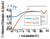
Figure 1: System’s and observer’s trajectories considering $\gamma_{f}=\gamma_{f}^{(\mathrm{analytical})}$ for the four generator states ($\delta,\omega,e_{q}^{\prime},e_{d}^{\prime}$). Similar state estimation results are obtained when using numerical Lipschitz constants after obtaining the corresponding observer gain $\bm{L}$.

VI Numerical Simulations

This section investigates the property and characteristic of the proposed analytical and numerical methods to determine the corresponding Lipschitz constants for $\bm{f}(\cdot)$ and $\bm{h}(\cdot)$. First, we compare the values of Lipschitz constants obtained from using both methods and second, explore the impact of the potentially conservative analytical Lipschitz constants on the design of asymptotic observers for the nonlinear generator with PMU measurement models (6b), with the objective of performing DSE.

VI-A Power System Parameters and Setup

We test the proposed approaches on the 16-machine, 68-bus system that is extracted from the PST toolbox [19] by considering Generator 16 in the network. The parameters are obtained from [19]. The input vector $\bm{u}$, including $T_{\mathrm{m}i}$, $E_{\mathrm{fd}i}$, $i_{\mathrm{R}i}$, and $i_{\mathrm{I}i}$ are obtained from simulations of the whole system in which each generator is using a transient model with IEEE Type DC1 excitation system and a simplified turbine-governor system [3]. To obtain lower and upper bounds on the state $\bm{x}$ and input $\bm{u}$, their minima and maxima are measured. All simulations are conducted by using MATLAB R2016b running on a 64-bit Windows 10 with 3.4GHz Intel^R Core^TM i7-6700 CPU and 16 GB of RAM. We use YALMIP [20] as the interface and MOSEK [21] solver to get the solutions of the LMI required by the DSE and observer.

VI-B Lipschitz Constants Computation

This section is devoted to determine Lipschitz constants of $\bm{f}(\cdot)$ and $\bm{h}(\cdot)$ given the generator parameters and operational range. First, we compute the analytical Lipschitz constants $\gamma_{f}^{(\mathrm{analytical})}$ and $\gamma_{h}^{(\mathrm{analytical})}$ by using applying (12a) and (12b) from Theorem 1. Second, we implement Algorithm 1 to compute numerical approximations of Lipschitz constants of $\bm{f}(\cdot)$ and $\bm{h}(\cdot)$. For these approximations, we utilize three different methods to generate the sampled points: random, Sobol, and Halton sequences. By generating $2000$ sample points inside the sets $\mathbfcal{X}$ and $\mathbfcal{U}$, we run the algorithm ten times to minimize the effect of randomization. The corresponding MATLAB functions used to generate these points are rand, sobolset, and haltonset. The results are given in Table I, where the mean values of the approximated Lipschitz constants $\gamma_{f,h}^{(\mathrm{numerical})}$ are compared with the analytical Lipschitz constants.

TABLE I: Analytical versus Numerical Lispchitz Constants.

Constant	Analytical	Random	Sobol	Halton
$\gamma_{f}$	715.395	19.802	20.128	20.131
$\gamma_{h}$	5.390	1.631	1.629	1.630

From this table, we observe that the analytical Lipschitz constants are much higher than the numerical ones, especially for $\gamma_{f}$. This is the case because the analytical Lipschitz constants given in (12) do not necessarily give the best ones, and thus serve as upper bounds for the numerical Lipschitz constants. We found that the high values are also due to the large operational range of the fourth control input ($i_{I}$) which significantly increases $\gamma_{f}^{\mathrm{(analytical)}}$. Amid this discrepancy, $\gamma_{f}^{(\mathrm{analytical})}$ and $\gamma_{f}^{(\mathrm{numerical})}$ are tested in the next section for performing DSE on a single generator. Specifically, we investigate whether these conservative analytical constants can be useful to perform DSE. We also observe that using LDS here did not have a drastic impact on the computation of the numerical Lipschitz constants—when compared with random sampling inside $\mathbfcal{X}$ and $\mathbfcal{U}$. To the best of our knowledge, one important feature of LDS for this particular purpose is that the approximated Lipschitz constants will converge to the actual ones as the number of sample point increases (assuming that $\bm{f}(\cdot)$ and $\bm{h}(\cdot)$ have continuous partial derivatives), which may or may not be the case for random sampling.

VI-C Generator DSE Using Lipschitz-Based Observer

In this simulation, we compare two different scenarios where the first one uses $\gamma_{f}^{(\mathrm{analytical})}=715.395$ whereas the other uses $\gamma_{f}^{(\mathrm{numerical})}=20.131$, which is the result from particularly using Halton sequence from Table I. Note that when simulating the DSE method through the observer (15), the nonlinear model of the output equation for both system and observer are used, i.e., $\bm{y}=\bm{h}(\bm{x},\bm{u})$ and $\hat{\bm{y}}=\bm{h}(\hat{\bm{x}},\bm{u})$.

Fig. 1 depicts the state estimation trajectories in comparison with the system’s trajectories given the analytical Lipschitz constant. Note that we have used significantly different initial conditions $\hat{\bm{x}}(0)$ for the observer, in comparison with the generator’s actual initial conditions (this can also be seen from Fig. 1). The simulation using the numerical Lipschitz constant exhibits very similar results. This implies that—for this specific test at least—both analytical and numerical Lipschitz constants can be utilized for performing DSE via Lipschitz-based nonlinear observers, and while the analytical Lipschitz constant was in fact large, it hinders neither finding a feasible solution for the LMI (16) nor obtaining asymptotically stable estimation error.

VII Summary, Closing Remarks, and Future Work

Motivated by the need to study higher-order nonlinear, dynamic models of power networks, this paper deals with the problem of determining the Lipschitz constants for fourth order generator dynamics with PMU measurements, which leads to the investigation of different methods to compute Lipschitz constants: analytical formulation and numerical algorithm based on low discrepancy sampling methods. Numerical tests showcase the discrepancy between the analytical and numerical methods, and applications to DSE of generator states given PMU measurements are provided.

We conclude the paper with the following remarks. (a) Albeit conservative, Theorem 1 and the analytical Lipschitz constants give confidence in applying Lipschitz-based estimators—and potentially state-feedback controllers for the nonlinear power network. (b) Although it is worried that large Lipschitz constants can impede the application of Lipschitz-based observers [11], we found that this may not always be the case, at least for performing DSE on a single generator. (c) Using LDS, in comparison with random sequences, does not seem to highly impact the values of numerical Lipschitz constants. The above observations (a)–(c) are, however, not thoroughly conclusive. Future work will focus on performing extensive numerical tests for various generators and operating conditions, as well as designing robust observers that consider nonlinear PMU measurement model under uncertainty.

Appendix A Single Generator State-Space Parameters

Constants $\alpha_{1,\ldots,10}$ and $\beta_{1,2}$ are given as:

$$\alpha_{1}=\omega_{0},\;\alpha_{2}=\frac{\omega_{0}}{2H_{i}},\;\alpha_{3}=\frac{\omega_{0}}{2H_{i}}\left(\frac{S_{\textrm{B}}}{S_{\textrm{N}i}}\right)$$

$$\alpha_{4}=\frac{\omega_{0}}{2H_{i}}\left(\frac{S_{\textrm{B}}}{S_{\textrm{N}i}}\right)^{2}(x^{\prime}_{\textrm{q}i}-x^{\prime}_{\textrm{d}i}),\;\alpha_{5}=\frac{K_{\textrm{D}i}}{2H_{i}},\;\alpha_{6}=\frac{K_{\textrm{D}i}}{2H_{i}}\omega_{0}$$

$$\alpha_{7}=\frac{1}{T^{\prime}_{\textrm{d0}i}},\;\alpha_{8}=\frac{1}{T^{\prime}_{\textrm{d0}i}}\left(\frac{S_{\textrm{B}}}{S_{\textrm{N}i}}\right)(x_{\textrm{d}i}-x^{\prime}_{\textrm{d}i}),\;\alpha_{9}=\frac{1}{T^{\prime}_{\textrm{q0}i}}$$

$$\alpha_{10}=\frac{1}{T^{\prime}_{\textrm{q0}i}}\left(\frac{S_{\textrm{B}}}{S_{\textrm{N}i}}\right)(x_{\textrm{q}i}-x^{\prime}_{\textrm{q}i}),\;\beta_{1}=\frac{1}{2}\left(\frac{S_{\textrm{B}}}{S_{\textrm{N}i}}\right)(x^{\prime}_{\textrm{q}i}-x^{\prime}_{\textrm{d}i})$$

$$\beta_{2}=\frac{1}{2}\left(\frac{S_{\textrm{B}}}{S_{\textrm{N}i}}\right)(x^{\prime}_{\textrm{q}i}+x^{\prime}_{\textrm{d}i}).$$

The state-space matrices $\bm{A},\bm{B}_{u},$ and $\bm{D}_{u}$ are given as

$$\bm{A}= \begin{bmatrix}0&1&0&0\\ 0&-\alpha_{5}&0&0\\ 0&0&-\alpha_{7}&0\\ 0&0&0&-\alpha_{9}\end{bmatrix},\;\bm{B_{\mathrm{u}}}=\begin{bmatrix}0&0&0&0\\ \alpha_{2}&0&0&0\\ 0&\alpha_{7}&0&0\\ 0&0&0&0\end{bmatrix}$$

$$\bm{D_{\mathrm{u}}}= \begin{bmatrix}0&0&0&\beta_{2}\\ 0&0&-\beta_{2}&0\end{bmatrix}.\;$$

References

• [1] P. Kundur, N. J. Balu, and M. G. Lauby, Power system stability and control.   McGraw-hill New York, 1994, vol. 7.
• [2] P. W. Sauer, M. Pai, and J. H. Chow, Power system dynamics and stability: with synchrophasor measurement and power system toolbox.   John Wiley & Sons, 2017.
• [3] J. Qi, A. F. Taha, and J. Wang, “Comparing kalman filters and observers for power system dynamic state estimation with model uncertainty and malicious cyber attacks,” IEEE Access, vol. 6, pp. 77 155–77 168, 2018.
• [4] E. Ghahremani and I. Kamwa, “Dynamic state estimation in power system by applying the extended kalman filter with unknown inputs to phasor measurements,” IEEE Transactions on Power Systems, vol. 26, no. 4, pp. 2556–2566, Nov. 2011.
• [5] J. Zhao, M. Netto, and L. Mili, “A robust iterated extended kalman filter for power system dynamic state estimation,” IEEE Trans. Power Syst., vol. 32, no. 4, pp. 3205–3216, July 2017.
• [6] N. Zhou, D. Meng, and S. Lu, “Estimation of the dynamic states of synchronous machines using an extended particle filter,” IEEE Transactions on Power Systems, vol. 28, no. 4, pp. 4152–4161, Nov. 2013.
• [7] J. Qi, K. Sun, J. Wang, and H. Liu, “Dynamic state estimation for multi-machine power system by unscented kalman filter with enhanced numerical stability,” IEEE Transactions on Smart Grid, vol. 9, no. 2, pp. 1184–1196, Mar. 2018.
• [8] A. F. Taha, J. Qi, J. Wang, and J. H. Panchal, “Risk mitigation for dynamic state estimation against cyber attacks and unknown inputs,” IEEE Trans. Smart Grid, vol. 9, no. 2, pp. 886–899, Mar. 2018.
• [9] A. F. Taha, M. Bazrafshan, S. Nugroho, N. Gatsis, and J. Qi, “Robust control architectures for renewable-integrated power networks using convex approximations,” arXiv preprint arXiv:1802.09071, 2018.
• [10] M. Khatibi and S. Ahmed, “Optimal resilient defense strategy against false data injection attacks on power system state estimation,” in 2018 IEEE Power Energy Society Innovative Smart Grid Technologies Conference (ISGT), Feb 2018, pp. 1–5.
• [11] M. Abbaszadeh and H. J. Marquez, “Nonlinear observer design for one-sided lipschitz systems,” in American Control Conference (ACC), 2010.   IEEE, 2010, pp. 5284–5289.
• [12] G. Phanomchoeng and R. Rajamani, “Observer design for lipschitz nonlinear systems using riccati equations,” in American Control Conference (ACC), 2010.   IEEE, 2010, pp. 6060–6065.
• [13] M. Jin, H. Feng, and J. Lavaei, “Multiplier-based observer design for large-scale Lipschitz systems,” 2018. [Online]. Available: http://www.jinming.tech/papers/Observer_2018_1.pdf
• [14] D. D. Siljak, D. M. Stipanovic, and A. I. Zecevic, “Robust decentralized turbine/governor control using linear matrix inequalities,” IEEE Transactions on Power Systems, vol. 17, no. 3, pp. 715–722, 2002.
• [15] J. Lian, S. Wang, R. Diao, and Z. Huang, “Decentralized robust control for damping inter-area oscillations in power systems,” arXiv preprint arXiv:1701.02036, 2017.
• [16] I. L. Dalal, D. Stefan, and J. Harwayne-Gidansky, “Low discrepancy sequences for monte carlo simulations on reconfigurable platforms,” in Application-Specific Systems, Architectures and Processors, 2008. ASAP 2008. International Conference on.   IEEE, 2008, pp. 108–113.
• [17] A. Chakrabarty, V. Dinh, M. J. Corless, A. E. Rundell, S. H. Żak, and G. T. Buzzard, “Support vector machine informed explicit nonlinear model predictive control using low-discrepancy sequences,” IEEE Transactions on Automatic Control, vol. 62, no. 1, pp. 135–148, Jan 2017.
• [18] J. Cheng and M. J. Druzdzel, “Computational investigation of low-discrepancy sequences in simulation algorithms for bayesian networks,” in Proceedings of the Sixteenth conference on Uncertainty in artificial intelligence.   Morgan Kaufmann Publishers Inc., 2000, pp. 72–81.
• [19] J. H. Chow and K. W. Cheung, “A toolbox for power system dynamics and control engineering education and research,” Power Systems, IEEE Transactions on, vol. 7, no. 4, pp. 1559–1564, 1992.
• [20] J. Löfberg, “Yalmip: A toolbox for modeling and optimization in matlab,” in Proc. IEEE Int. Symp. Computer Aided Control Systems Design.   IEEE, 2004, pp. 284–289.
• [21] E. D. Andersen and K. D. Andersen, “The mosek interior point optimizer for linear programming: an implementation of the homogeneous algorithm,” in High performance optimization.   Springer, 2000, pp. 197–232.