A Fully Differentiable Beam Search Decoder

Abstract

We introduce a new beam search decoder that is fully differentiable, making it possible to optimize at training time through the inference procedure. Our decoder allows us to combine models which operate at different granularities (e.g. acoustic and language models). It can be used when target sequences are not aligned to input sequences by considering all possible alignments between the two. We demonstrate our approach scales by applying it to speech recognition, jointly training acoustic and word-level language models. The system is end-to-end, with gradients flowing through the whole architecture from the word-level transcriptions. Recent research efforts have shown that deep neural networks with attention-based mechanisms are powerful enough to successfully train an acoustic model from the final transcription, while implicitly learning a language model. Instead, we show that it is possible to discriminatively train an acoustic model jointly with an explicit and possibly pre-trained language model.

1 Introduction

End-to-end models for tasks such as automatic speech recognition require the use of either structured loss functions like Connectionist Temporal Classification (Graves et al., 2006) or unstructured models like sequence-to-sequence (Sutskever et al., 2014) which leverage an attention mechanism (Bahdanau et al., 2014) to learn an implicit alignment. Both these types of models suffer from an exposure bias and a label bias problem.

Exposure-bias results from the mismatch between how these models are trained and how they are used at inference (Ranzato et al., 2016; Wiseman and Rush, 2016; Baskar et al., 2018). While training, the model is never exposed to its own mistakes since it uses the ground-truth target as guidance. At inference the target is unavailable and a beam search is typically used, often with the constraints of either a lexicon, a transition model, or both. The model must rely on past predictions to inform future decisions and may not be robust to even minor mistakes.

Label-bias occurs when locally normalized transition scores are used (LeCun et al., 1998; Lafferty et al., 2001; Bottou and LeCun, 2005). Local normalization causes outgoing transitions at a given time-step to compete with one another. A symptom of this is that it can be difficult for the model to revise its past predictions based on future observations. As a consequence, globally normalized models are strictly more powerful than locally normalized models (Andor et al., 2016).

In this work we build a fully differentiable beam search decoder (DBD) which can be used to efficiently approximate a powerful discriminative model without either exposure bias or label bias. We alleviate exposure bias by performing a beam search which includes the constraints from a lexicon and transition models. In fact, DBD can also jointly train multiple models operating at different granularities (e.g. token and word-level language models). The DBD avoids the label bias problem since it uses unnormalized scores and combines these scores into a global (sequence-level) normalization term.

Our differentiable decoder can handle unaligned input and output sequences where multiple alignments exist for a given output. The DBD model also seamlessly and efficiently trains token-level, word-level or other granularity transition models on their own or in conjunction. Connectionist Temporal Classification (CTC) (Graves et al., 2006) can handle unaligned sequences and is commonly used in automatic speech recognition (ASR) (Amodei et al., 2016) and other sequence labeling tasks (Liwicki et al., 2007; Huang et al., 2016). The Auto Segmentation criterion (ASG) (Collobert et al., 2016) can also deal with unaligned sequences. However, neither of these criteria allow for joint training of arbitrary transition models.

Because DBD learns how to aggregate scores from various models at training time, it avoids the need for a grid search over decoding parameters (e.g. language model weights and word insertion terms) on a held-out validation set at test time. Furthermore, all of the scores used by the differentiable decoder are unnormalized and we thus discard the need for costly normalization terms over large vocabulary sizes. In fact, when using DBD, training a language model with a two-million word vocabulary instead of a two-thousand word vocabulary would incur little additional cost.

We apply DBD to the task of automatic speech recognition and show competitive performance on the Wall Street Journal (WSJ) corpus (Paul and Baker, 1992). Compared to other baselines which only use the acoustic data and transcriptions, our model achieves word error rates which are comparable to state-of-the-art. We also show that DBD enables much smaller beam sizes and smaller and simpler models while achieving lower error rates. This is crucial, for example, in deploying models with tight latency and throughput constraints.

In the following section we give a description of the exact discriminative model we wish to learn and in Sections 3 and 4 show how a differentiable beam search can be used to efficiently approximate this model. In Section 4 we also explain the target sequence-tracking technique which is critical to the success of DBD. We explain how DBD can be applied to the task of ASR in Section 5 along with a description of the acoustic and language models (LMs) we consider. Section 6 describes our experimental setup and results on the WSJ speech recognition task. In Section 7 we put DBD in context with prior work and conclude in Section 8.

2 Model

In the following, we consider an input sequence ${\mathbf{X}}=[X_{1},\,\dots,\,X_{T}]$, and its corresponding target sequence $\tau$. We also denote a token-level alignment over the $T$ acoustic frames as $\pi=[\pi_{1},\,\dots,\,\pi_{T}]$. An alignment leading to the target sequence of words $\tau$ is denoted as $\pi^{\tau}$. The conditional likelihood of $\tau$ given the input ${\mathbf{X}}$ is then obtained by marginalizing over all possible alignments $\pi$ leading to $\tau$:

$$\log P(\tau|{\mathbf{X}})=\log\sum_{\forall\pi^{\tau}}P(\pi^{\tau}|{\mathbf{X}})\,.$$ (1)

In the following, we consider a scoring function $f^{t}(i|{\mathbf{X}})$ which outputs scores for each frame $t\in[1,\dots,T]$ and each label $i\in{\cal D}$ in a token set. We also consider a token transition model $g(i,j)$ (we stick to a bigram for the sake of simplicity) and a word transition model $h(\cdot)$. Given an input sequence ${\mathbf{X}}$, an alignment $\pi^{\tau}$ is assigned an unnormalized score $s(\pi^{\tau}|{\mathbf{X}})$ obtained by summing up frame scores, token-level transition scores along $\pi^{\tau}$ and the word-level transition model score:

$$s(\pi^{\tau}|{\mathbf{X}})=\sum_{t=1}^{T}f^{t}(\pi^{\tau}_{t}|{\mathbf{X}})+g(\pi^{\tau}_{t}|\pi^{\tau}_{t-1})+h(\tau)\,.$$ (2)

It is important to note that the frame scores and transition scores are all unnormalized. Hence, we do not require any transition model weighting as the model will learn the appropriate scaling. Also, $P(\pi^{\tau}|{\mathbf{X}})$ in Equation (1) is obtained by performing a sequence-level normalization, applying a softmax over all alignment scores $s(\pi^{\eta}|{\mathbf{X}})$ for all possible valid sequences of words $\eta$ ($\eta$ necessarily include $\tau$):

$$\log P(\pi^{\tau}|{\mathbf{X}})=s(\pi^{\tau}|{\mathbf{X}})-\log\sum_{\forall\eta,\,\forall\pi^{\eta}}e^{s(\pi^{\eta}|{\mathbf{X}})}\,.$$ (3)

Combining Equation (1) and Equation (3), and introducing the operator $\operatorname*{logadd}(a,\,b)=\log(e^{a}+e^{b})$ for convenience, our model can be summarized as:

$$\log P(\tau|{\mathbf{X}})=\operatorname*{logadd}_{\forall\pi^{\tau}}s(\pi^{\tau}|{\mathbf{X}})-\operatorname*{logadd}_{\forall\eta,\,\forall\pi^{\eta}}s(\pi^{\eta}|{\mathbf{X}})\,.$$ (4)

Our goal is to optimize jointly the scoring function and the transition models (token-level and word-level) by maximizing this conditional likelihood over all labeled pairs $({\mathbf{X}},\,\tau)$ available at training time. In Equation (4), it is unfortunately intractable to exactly compute the $\operatorname*{logadd}()$ over all possible sequences $\eta$ of valid words. In the next section, we will relate this likelihood to what is computed during decoding at inference and then show how it can be approximated efficiently. In Section 4, we will show how it can be efficiently optimized.

3 Decoding

At inference, given an input sequence ${\mathbf{X}}$, one needs to find the best corresponding word sequence $\tau^{\star}$. A popular decoding approach is to define the problem formally as finding $\operatorname*{argmax}_{\tau}s(\pi^{\tau}|{\mathbf{X}})$, implemented as a Viterbi search. However, this approach takes in account only the best alignment $\pi^{\tau}$ leading to $\tau$. Keeping in mind the normalization in Equation (4), and following the footsteps of (Bottou, 1991), we are interested instead in finding the $\tau$ which maximizes the Forward score:

$$\begin{split}\max_{\tau}\log P(\tau|{\mathbf{X}})&=\max_{\tau}\operatorname*{logadd}_{\forall\pi^{\tau}}s(\pi^{\tau}|{\mathbf{X}})\\ \ &\approx\max_{\tau\in{\cal B}}\operatorname*{logadd}_{\forall\pi^{\tau}\in{\cal B}}s(\pi^{\tau}|{\mathbf{X}})\,.\end{split}$$ (5)

The first derivation in Equation (5) is obtained by plugging in Equation (4) and noticing that the normalization term $\operatorname*{logadd}_{\forall\eta}()$ is constant with respect to $\tau$. As the search over all possible sequences of words is intractable, one performs a beam search, which results in a final set of hypotheses ${\cal B}$. For each hypothesis in the beam ($\tau\in{\cal B}$), note that only the most promising alignments leading to this hypothesis will also be in the beam ($\forall\pi^{\tau}\in{\cal B}$); in contrast to pure Viterbi decoding, these alignments are aggregated through a $\operatorname*{logadd}()$ operation instead of a $\max()$ operation.

Our beam search decoder uses a word lexicon (implemented as a trie converting sequences of tokens into words) to constrain the search to only valid sequences of words $\tau$. The decoder tracks hypotheses $\tau$ with the highest scores by bookkeeping tuples of “(lexicon state, transition model state, score)” as it iterates through time. At each time step, hypotheses with the same transition model state and lexicon state are merged into the top scoring hypothesis with this state. The score of the resulting hypothesis is the $\operatorname*{logadd}()$ of the combined hypotheses.

3.1 Decoding to compute the likelihood normalization

The normalization term computed over all possible valid sequence of words $\eta$ in the conditional likelihood Equation (4) can be efficiently approximated by the decoder, subject to a minor modification.

$$\begin{split}\operatorname*{logadd}_{\forall\eta,\,\forall\pi^{\eta}}s(\pi^{\eta}|{\mathbf{X}})&=\operatorname*{logadd}_{\forall\eta}\operatorname*{logadd}_{\forall\pi^{\eta}}s(\pi^{\eta}|{\mathbf{X}})\\ &\approx\operatorname*{logadd}_{\forall\eta\in{\cal B}}\operatorname*{logadd}_{\forall\pi^{\eta}\in{\cal B}}s(\pi^{\eta}|{\mathbf{X}})\,,\end{split}$$ (6)

where ${\cal B}$ is the set of hypotheses retained by the decoder beam. Compared to Equation (5), the only change in Equation (6) is the final “aggregation” of the hypotheses in the beam: at inference, one performs a $\max()$ operation, while to compute the likelihood normalization one performs a $\operatorname*{logadd}()$.

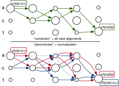
Figure 1: An example of the DBD computation of the loss (Equation (7)), with a target transcription of “a cat”, using a lexicon {a, cat}, 5 frames in total, and a word-level bigram LM $h(\cdot)$. Circle sizes are proportional to the AM score and paths through the graph are aggregated with a $\operatorname*{logadd}$. The first term (maximized, “numerator”) corresponds to all valid alignments (in green). The second term corresponds to the beam search which is used to construct the denominator (Equation (8)). Dashed arrows denote transitions not included in the beam. Multiple alignments leading to the same word are merged, and the LM scores are added (rounded rectangles) as words are considered in the beam.

4 Differentiable Decoding

As mentioned in Section 2, we aim to jointly train the scoring function and the transition models (token-level and word-level) by maximizing the conditional likelihood in Equation (4) over all training pairs $({\mathbf{X}},\,\tau)$. Leveraging the decoder to approximate the normalization term (with Equation (6)), and denoting $\pi\in{\cal T}_{\tau}$ and $\pi\in{\cal B}$ for all alignments leading to the target and all alignments in the beam respectively, this corresponds to maximizing:

$$\log P(\tau|{\mathbf{X}})=\operatorname*{logadd}_{\forall\pi\in{\cal T}_{\tau}}s(\pi|{\mathbf{X}})-\operatorname*{logadd}_{\forall\pi\in{\cal B}}s(\pi|{\mathbf{X}})\,.$$ (7)

This approximated conditional likelihood can be computed and differentiated in a tractable manner. The $\operatorname*{logadd}_{\pi\in{\cal T}_{\tau}}$ can be exactly evaluated via dynamic programming (the Forward algorithm). The normalization term $\operatorname*{logadd}_{\pi\in{\cal B}}$ is computed efficiently with the decoder. Interestingly, both of these procedures (the Forward algorithm and decoding) only invoke additive, multiplicative and $\operatorname*{logadd}()$ operations in an iterative manner. In that respect, everything is fully differentiable, and one can compute the first derivatives $\partial\log P(\tau|{\mathbf{X}})/\partial f_{t}(i|{\mathbf{X}})$, $\partial\log P(\tau|{\mathbf{X}})/\partial g(i|j)$, $\partial\log P(\tau|{\mathbf{X}})/\partial h$ by backpropagating through the Forward and decoder iterative processes.

4.1 On the normalization approximation

In practice, the normalization approximation shown in Equation (7) is unfortunately inadequate. Indeed, the beam ${\cal B}$ may or may not contain some (or all) character alignments found in ${\cal T}_{\tau}$. We observe that models with improper normalization fail to converge as everything (scoring function and transition models) outputs unnormalized scores. We correct the normalization by considering instead the $\operatorname*{logadd}()$ over $({\cal B}\setminus{\cal B}\cap{\cal T}_{\tau})\cup{\cal T}_{\tau}$. This quantity can be efficiently computed using the following observation:

$$\begin{split}\operatorname*{logadd}_{\forall\pi\in({\cal B}\setminus{\cal B}\cap{\cal T}_{\tau})\cup{\cal T}_{\tau}}s(\pi|{\mathbf{X}})=\log(&e^{\operatorname*{logadd}_{\forall\pi\in{\cal B}}s(\pi|{\mathbf{X}})}\\ -&e^{\operatorname*{logadd}_{\forall\pi\in{\cal B}\cap{\cal T}_{\tau}}s(\pi|{\mathbf{X}})}\\ +&e^{\operatorname*{logadd}_{\forall\pi\in{\cal T}_{\tau}}s(\pi|{\mathbf{X}})})\,.\end{split}$$ (8)

The $\operatorname*{logadd}()$ terms over ${\cal B}$ and ${\cal T}_{\tau}$ are given by the decoder and the Forward algorithm respectively. The $\operatorname*{logadd}()$ term over ${\cal B}\cap{\cal T}_{\tau}$ can also be computed by the decoder by tracking alignments in the beam which correspond to the ground truth $\tau$. While this adds extra complexity to the decoder, it is an essential feature for successful training.

4.2 On the implementation

Our experience shows that implementing an efficient differentiable version of the decoder is tricky. First, it is easy to miss a term in the gradient given the complexity of the decoding procedure. It is also difficult to check the accuracy of the gradients by finite differences (and thus hard to find mistakes) given the number of operations involved in a typical decoding pass. To ensure the correctness of our derivation, we first implemented a custom C++ autograd (operating on scalars, as there are no vector operations in the decoder). We then designed a custom version of the differentiable decoder (about 10$\times$ faster than the autograd version) which limits memory allocation and checked the correctness of the gradients via the autograd version.

5 Application to Speech Recognition

In a speech recognition framework, the input sequence ${\mathbf{X}}$ is an acoustic utterance, and the target sequence $\tau$ is the corresponding word transcription. Working at the word level is challenging, as corpora are usually not large enough to model rare words properly. Also, some words in the validation or test sets may not be present at training time. Instead of modeling words, one considers sub-word units – like phonemes, context-dependent phonemes, or characters. In this work, we use characters for simplicity. Given an acoustic sequence ${\mathbf{X}}$, character-level alignments corresponding to the word transcription $\tau$ are $\pi^{\tau}$. The correct character-level alignment is unknown. The scoring function $f^{t}(\pi^{\tau}_{t}|{\mathbf{X}})$ is an acoustic model predicting character scores at each frame $X_{t}$ of the utterance $X$. The transition model $g(i|j)$ learns a character-level language model, and the word transition model $h(\tau)$ is a word language model.

Both the acoustic and language models can be customized in our approach. We use a simple ConvNet architecture (leading to a reasonable end-to-end word error rate performance) for the acoustic model, and experimented with a few different language models. We now describe these models in more details.

5.1 Acoustic Model

We consider a 1D ConvNet for the acoustic model (AM), with Gated Linear Units (GLUs) (Dauphin et al., 2017) for the transfer function and dropout as regularization. Given an input ${\mathbf{X}}^{l}$, the $l^{th}$ layer of a Gated ConvNet computes

$$h_{l}({\mathbf{X}}^{l})=({\mathbf{X}}^{l}\ast\mathbf{W}^{l}+\mathbf{b})\otimes\sigma({\mathbf{X}}^{l}\ast\mathbf{W^{\prime}}^{l}+\mathbf{b^{\prime}})\,,$$

where $\mathbf{W}^{l}$, $\mathbf{b}$ and $\mathbf{W^{\prime}}^{l}$, $\mathbf{b^{\prime}}$ are trainable parameters of two different convolutions. As $\sigma()$ is the sigmoid function, and $\otimes$ is the element-wise product between matrices, GLUs can be viewed as a gating mechanism to train deeper networks. Gated ConvNets have been shown to perform well on a number of tasks, including speech recognition (Liptchinsky et al., 2017). As the differentiable decoder requires heavy compute, we bootstrapped the training of the acoustic model with ASG. The ASG criterion is similar to Equation (3) but the normalization term is taken over all sequences of tokens

$$\log P(\pi^{\tau}|{\mathbf{X}})=s(\pi^{\tau}|{\mathbf{X}})-\log\sum_{\forall\pi}e^{s(\pi|{\mathbf{X}})}$$ (9)

with the alignment score is given by

$$s(\pi^{\tau}|{\mathbf{X}})=\sum_{t=1}^{T}f^{t}(\pi^{\tau}_{t}|{\mathbf{X}})+g(\pi^{\tau}_{t}|\pi^{\tau}_{t-1})$$ (10)

which does not include a word language model.

5.2 Language Models

The character language model as shown in Equation (2) was chosen to be a simple trainable scalar $g(i|j)=\lambda_{ij}$. We experimented with several word language models:

1. A zero language model $h(\tau)=0$. This special case is a way to evaluate how knowing the lexicon can help the acoustic model training. Indeed, even when there is no language model information, the normalization shown in Equation (4) still takes in account the available lexicon. Only sequences of letters $\pi$ leading to a valid sequence of words $\tau$ are considered (compared to any sequence of letters, as in ASG or LF-MMI).

2. A pre-trained language model, possibly on data not available for the acoustic model training. We considered in this case

   $$h(\tau)=\lambda\log P_{lm}(\tau)+\gamma\,,$$ (11)

   where $P_{lm}(\tau)$ is the pre-trained language model. The language model weight $\lambda$ and word insertion score $\gamma$ are parameters trained jointly with the acoustic model.

3. A bilinear language model. Denoting the sequence of words $\tau=[\tau_{1},\,\dots,\,\tau_{N}]$, we consider the unnormalized language model score:

   $$h(\tau)=w_{\tau_{N}}^{T}\sum_{n=1}^{K}\mathbf{M}_{n}w_{\tau_{N-n}}\,,$$ (12)

   where $K\geq 2$ is the order of the language model. The word embeddings $w_{i}\in\mathbb{R}^{d}$ ($d$ to be chosen) and the projection matrices $M_{i}\in\mathbb{R}^{d\times d}$ are trained jointly with the acoustic model. It is worth mentioning that the absence of normalization makes this particular language model efficient.

6 Experiments

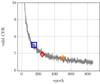
(a)

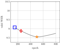
(b)

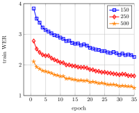
(c)

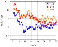
(d)

Figure 2: Performance of the 10M parameters ConvNet, with respect to training epochs over WSJ. ASG baseline valid error is shown CER (a) and WER (b). Each ASG WER was obtained by running a full grid search (beam size 8000). DBD train (c) and valid (d) WER: three DBD runs were forked from the ASG baseline at epochs 150, 250 and 500 (see colors/shapes) and trained with beam size 500.

We performed experiments with WSJ (about $81$h of transcribed audio data). We consider the standard subsets si284, nov93dev and nov92 for training, validation and test, respectively. We use log-mel filterbanks as features fed to the acoustic model, with 40 filters of size 25ms, strided by 10ms. We consider an end-to-end setup, where the token set ${\cal D}$ (see Section 2) includes English letters (a-z), the apostrophe and the period character, as well as a space character, leading to 29 different tokens. No data augmentation or speaker adaptation was performed. As WSJ ships with both acoustic training data and language-model specific training data, we consider two different training setups:

1. Language models are pre-trained (see Equation (11)) with the full available language model data. This allows us to demonstrate that our approach can tune automatically the language model weight and leverage the language model information during the training of the acoustic model.

2. Both acoustic and language models are trained with acoustic (and corresponding transcription) data only. This allows us to compare with other end-to-end work where only the acoustic data was used.

Pre-trained language models are n-gram models trained with KenLM (Heafield, 2011). The word dictionary contains words from both the acoustic and language model data. We did not perform any thresholding, leading to about 160K distinct words.

All the models are trained with stochastic gradient descent (SGD), enhanced with gradient clipping (Pascanu et al., 2013) and weight normalization (Salimans and Kingma, 2016). In our experience, these two improvements over vanilla SGD allow higher learning rates, and lead to faster and more stable convergence. Without weight normalization we found GLU-ConvNets very challenging to train. We use batch training (16 utterances at once), sorting inputs by length prior to batching for efficiency. Both the neural network acoustic model and the ASG criterion run on a single GPU. The DBD criterion is CPU-only. With ASG, a single training epoch over WSJ takes just a few minutes, while it takes about an hour with DBD.

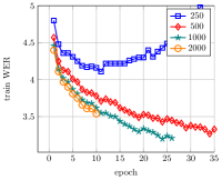
(a)

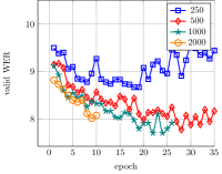
(b)

Figure 3: Training DBD with different beam size, showing train (a) and valid (b) WER, for the 7.5M parameters model on WSJ.

6.1 Leveraging Language-Model Data

In speech recognition, it is typical to train the acoustic model and the language model separately. The language model can take advantage of large text-only corpora. At inference, both models are combined through the decoding procedure (maximizing Equation (5)). Hyper-parameters combining the language model (as in Equation (11)) are tuned through a validation procedure (e.g. grid-search).

We first performed an extensive architecture search, training models with ASG and selecting a baseline model as the one leading to the best validation character error rate (CER). Our best ConvNet acoustic model has 10M parameters and an overall receptive field of 1350ms. A 4-gram language model was trained over the text data provided with WSJ. A decoding grid search was then performed at several points during the acoustic model training Figure 2b). While CER and WER are correlated, the best WER did not correspond to the best CER (see Figure 2a and Figure 2b).

Table 1: Comparing WER performance of ASG with decoding grid-search, and DBD, on WSJ. We compare with standard end-to-end approaches, for reference.

Model	nov93dev	nov92
ASG 10M AM (beam size 8000)	8.5	5.6
ASG 10M AM (beam size 500)	8.9	5.7
ASG 7.5M AM (beam size 8000)	8.8	6.0
ASG 7.5M AM (beam size 500)	9.4	6.1
DBD 10M AM (beam size 500)	8.7	5.9
DBD 7.5M AM (beam size 500)	7.7	5.3
DBD 7.5M AM (beam size 1000)	7.7	5.1
Attention RNN+CTC		9.3
(3gram) (Bahdanau et al., 2016a)
CNN+ASG	9.5	5.6
(4-gram) (Zeghidour et al., 2018)
CNN+ASG (wav+convLM)	6.8	3.5
(Zeghidour et al., 2018)
RNN+E2E-LF-MMI (data augm.)		4.1
(+RNN-LM) (Hadian et al., 2018)
BLSTM+PAPB+CE		3.8
(RNN-LM) (Baskar et al., 2018)

As DBD training is time-consuming compared to ASG-training, we bootstrapped several DBD models from three different checkpoints of our ASG model (at epoch 125, 250 and 500). With DBD, the acoustic model is jointly fine-tuned with the weights of the language model shown in Equation (11). Figure 2c and Figure 2d show the training and validation WER with respect to number of epochs over WSJ. DBD converges quickly from the pre-trained ASG model, while many epochs (and a grid-search for the language model hyper-parameters) are required to match the same WER with ASG. When starting from later ASG epochs (250 and 500), DBD badly overfits to the training set.

To mitigate overfitting, we trained a variant of our 10M model where the receptive field was reduced to 870ms (leading to 7.5M parameters). Table 1 summarizes our results. While ASG is unable to match the WER performance of the 1450ms receptive field model, training with DBD leads to better performance, demonstrating the advantage of jointly training the acoustic model with the language model. Not only does DBD allow for more compact acoustic models, but also DBD-trained models require much smaller beam at decoding, which brings a clear speed advantage at inference.

Figure 3 shows the effect of the beam size during DBD training. Having too small a beam leads to model divergence. Training epoch times for beam sizes of 500, 1000 and 2000 are 35min, 90m and 180min respectively. In most experiments, we use a beam size of 500, as larger beam sizes led to marginal WER improvements. Although, in contrast to pipelines suffering from exposure bias (e.g. Koehn and Knowles, 2017), larger beams are always better.

6.2 Experimenting with Acoustic-Only Data

Recent work on WSJ has shown that end-to-end approaches are good at modeling acoustic data. Some of these works also demonstrated that with architectures powerful enough to capture long-range dependencies, end-to-end approaches can also implicitly model language, and push the WER even further down. DBD allows us to explicitly design acoustic and language models while training them jointly. We show in this section that with simple acoustic and language models, we can achieve WERs on par with existing approaches trained on acoustic-only data.

Table 2: WSJ performance (WER), using only the acoustic training data. ASG n-gram decoding hyper-parameters were tuned via grid-search. Beam size for both ASG and DBD was 500. Larger beam sizes with ASG did not lead to significant improvements.

Model	nov93dev	nov92
ASG (zero LM decoding)	18.3	13.2
ASG (2-gram LM decoding)	14.8	11.0
ASG (4-gram LM decoding)	14.7	11.3
DBD zero LM	16.9	11.6
DBD 2-gram LM	14.6	10.4
DBD 2-gram-bilinear LM	14.2	10.0
DBD 4-gram LM	13.9	9.9
DBD 4-gram-bilinear LM	14.0	9.8
RNN+CTC		30.1
(Graves and Jaitly, 2014)
Attention RNN+CTC		18.6
(Bahdanau et al., 2016a)
Attention RNN+CTC+TLE		17.6
(Bahdanau et al., 2016b)
Attn. RNN+seq2seq+CNN		9.6
(speaker adapt.) (Chan et al., 2017)
BLSTM+PAPB+CE		10.8
(Baskar et al., 2018)

In Table 2 we report standard baselines for this setup, as well as our own ASG baseline model, decoded with an n-gram trained only on acoustic data. We compare with DBD-trained models using the three different language models introduced in Section 5.2: (i) a zero language model, which allows us to leverage the word lexicon while training; (ii) n-gram language models, pre-trained on acoustic data (where the weighting is trained jointly with the acoustic model) and (iii) bilinear language models (where all the parameters are trained jointly with the acoustic model). Results show that only knowing the lexicon when training the acoustic model already greatly improves the WER over the baseline ASG model, where the lexicon is known only at test time. Jointly training a word language model with the acoustic model further reduces the WER.

7 Related Work

Our differentiable decoder belongs to the class of sequence-level training criteria, which includes Connectionist Temporal Classification (CTC) (Graves et al., 2006; Graves and Jaitly, 2014) and the Auto Segmentation (ASG) criterion (Collobert et al., 2016), as well as Minimum Bayes Risk (MBR and sMBR) (Goel and Byrne, 2000; Gibson and Hain, 2006; Sak et al., 2015; Prabhavalkar et al., 2018) and the Maximum Mutual Information (MMI) criterion (Bahl et al., 1986), amongst others. MMI and ASG are the closest to our differentiable decoder as they perform global (sequence- level) normalization, which should help alleviate the label bias problem (LeCun et al., 1998; Lafferty et al., 2001; Bottou and LeCun, 2005; Andor et al., 2016).

Both MBR and MMI are usually trained after (or mixed with) another sequence loss or a force-alignment phase. MMI maximizes the average mutual information between the observation ${\mathbf{X}}$ and its correct transcription $\tau$. Considering an HMM with states $S_{\tau}=[s^{\tau}_{1},\,\dots,\,s^{\tau}_{T}]$ for a given transcription $\tau$, MMI maximizes:

$$I(\tau,{\mathbf{X}})=\log P({\mathbf{X}}|S_{\tau})P(\tau)-\operatorname*{logadd}_{\eta}\log P({\mathbf{X}}|S_{\eta})P(\eta)\,.$$ (13)

In contrast to MMI, MBR techniques integrate over plausible transcriptions $\eta$, weighting each candidates by some accuracy $A(\tau,\,\eta)$ to the ground truth – computing $\sum_{\eta}e^{I(\eta,{\mathbf{X}})}A(\tau,\,\eta)$.

In a neural network context, one can apply Bayes’ rule to plug in the emission probabilities. Ignoring $P({\mathbf{X}})$, the term $\log P({\mathbf{X}}|s_{t})$ in Equation (13) is approximated by $\log P(s_{t}|{\mathbf{X}})-\log P(s)$, where $\log P(s_{t}|{\mathbf{X}})=f_{t}(s_{t}|{\mathbf{X}})$ (the emissions being normalized per frame), and $P(s)$ is estimated with the training data. Apart from this approximation, two differences with our differentiable decoder are critical:

• MMI considers normalized probabilities for both the acoustic and language model, while we consider unnormalized scores everywhere.

• MMI does not jointly train the acoustic and language models. MMI does come in different flavors though, with (fixed) token level (phone) language models and no lexicon, as found in lattice-free MMI (LF-MMI) (Povey et al., 2016), and even trained end-to-end without any alignments (EE-LF-MMI) as in (Hadian et al., 2018), with a pre-trained phone LM still.

ASG maximizes Equation (9) which is similar to Equation (4) but with two critical differences: (1) there is no word language model in Equation (2), and (2) the normalization term is not constrained to valid sequences of words but is over all possible sequences of letters, and thus can be computed exactly (as is the case for LF-MMI). Unlike ASG, CTC assumes output tokens are conditionally independent given the input and includes an optional blank which makes the graph less regular (Liptchinsky et al., 2017).

Because our work is end-to-end, it is also related to seq2seq learning (Sutskever et al., 2014; Bahdanau et al., 2014; Chan et al., 2017; Wiseman and Rush, 2016; Gehring et al., 2017), and in particular training with existing/external language models (Sriram et al., 2018). Closest to our work is (Baskar et al., 2018) that shares a similar motivation, training an acoustic model through beam search although its (1) loss includes an error rate (as MBR), (2) they consider partial hypotheses (promising accurate prefix boosting: PAPB), and in practice (3) they optimize a loss composing this beam search sequence score with the cross-entropy (CE).

In NLP, training with a beam search procedure is not new (Collins and Roark, 2004; Daumé III and Marcu, 2005; Wiseman and Rush, 2016). Of those, (Wiseman and Rush, 2016) is the closest to our work, training a sequence model through a beam-search with a global sequence score. To our knowledge, we are the first to train through a beam search decoder for speech recognition, where the multiplicity of gold transcription alignments makes the search more complex. Also related, several works are targeting the loss/evaluation mismatch (and sometimes exposure bias) through reinforcement learning (policy gradient) (Bahdanau et al., 2016b; Ranzato et al., 2016) even in speech recognition (Zhou et al., 2018).

Finally, our work makes a generic beam search differentiable end-to-end and so relates to relaxing the beam search algorithm itself (e.g. getting a soft beam through a soft argmax) (Goyal et al., 2018), although we use a discrete beam. Compared to differentiable dynamic programming (Mensch and Blondel, 2018; Bahdanau et al., 2016b), we use a $\operatorname*{logadd}$ where they use a softmax and we keep track of an n-best (beam) set while they use Viterbi-like algorithms.

8 Conclusion

We build a fully differentiable beam search decoder which is capable of jointly training a scoring function and arbitrary transition models. The DBD can handle unaligned sequences by considering all possible alignments between the input and the target. Key to this approach is a carefully implemented and highly optimized beam search procedure which includes a novel target sequence-tracking mechanism and an efficient gradient computation. As we show, DBD can scale to very long sequences with thousands of time-steps. We are able to perform a full training pass (epoch) through the WSJ data in about half-an-hour with a beam size of 500.

We show that the beam search decoder can be used to efficiently approximate a discriminative model which alleviates exposure bias from the mismatch between training and inference. We also avoid the label bias problem by using unnormalized scores and performing a sequence-level normalization. Furthermore, the use of unnormalized scores allows DBD to avoid expensive local normalizations over large vocabularies.

Since DBD jointly trains the scoring function and the transition models, it does away with the need for decoder hyper-parameter tuning on a held-out validation set. We also observe on the WSJ test set that DBD can achieve better WERs at a substantially smaller beam size (500 vs 8000) than a well tuned ASG baseline.

On the WSJ dataset, DBD allows us to train much simpler and smaller acoustic models with better error rates. One reason for this is that DBD can limit the competing outputs to only sequences consisting of valid words in a given lexicon. This frees the acoustic model from needing to assign lower probability to invalid sequences. Including an explicit language model further decreases the burden on the acoustic model since it does not need to learn an implicit language model. We show that models with fewer parameters and half the temporal receptive field can achieve equally good error rates when using DBD.

References

- Graves et al. (2006) Alex Graves, Santiago Fernández, Faustino Gomez, and Jürgen Schmidhuber. Connectionist temporal classification: labelling unsegmented sequence data with recurrent neural networks. In International Conference on Machine Learning (ICML), pages 369–376, 2006.
- Sutskever et al. (2014) Ilya Sutskever, Oriol Vinyals, and Quoc V Le. Sequence to sequence learning with neural networks. In Advances in neural information processing systems (NIPS), pages 3104–3112, 2014.
- Bahdanau et al. (2014) Dzmitry Bahdanau, Kyunghyun Cho, and Yoshua Bengio. Neural machine translation by jointly learning to align and translate. In International Conference on Learning Representations (ICLR), 2014.
- Ranzato et al. (2016) Marc’Aurelio Ranzato, Sumit Chopra, Michael Auli, and Wojciech Zaremba. Sequence level training with recurrent neural networks. In International Conference on Learning Representations (ICLR), 2016.
- Wiseman and Rush (2016) Sam Wiseman and Alexander M. Rush. Sequence-to-sequence learning as beam-search optimization. In Proceedings of the Conference on Empirical Methods in Natural Language Processing (EMNLP), pages 1296–1306. Association for Computational Linguistics, 2016. URL http://aclweb.org/anthology/D16-1137.
- Baskar et al. (2018) Murali Karthick Baskar, Lukáš Burget, Shinji Watanabe, Martin Karafiát, Takaaki Hori, and Jan Honza Černockỳ. Promising accurate prefix boosting for sequence-to-sequence ASR. arXiv preprint arXiv:1811.02770, 2018.
- LeCun et al. (1998) Y. LeCun, L. Bottou, Y. Bengio, and P. Haffner. Gradient-based learning applied to document recognition. Proceedings of the IEEE, 86(11):2278–2324, 1998.
- Lafferty et al. (2001) John D. Lafferty, Andrew McCallum, and Fernando C. N. Pereira. Conditional random fields: Probabilistic models for segmenting and labeling sequence data. In International Conference on Machine Learning (ICML), pages 282–289, 2001. URL http://dl.acm.org/citation.cfm?id=645530.655813.
- Bottou and LeCun (2005) Léon Bottou and Yann LeCun. Graph transformer networks for image recognition. Bulletin of the 55th Biennial Session of the International Statistical Institute (ISI), 2005.
- Andor et al. (2016) Daniel Andor, Chris Alberti, David Weiss, Aliaksei Severyn, Alessandro Presta, Kuzman Ganchev, Slav Petrov, and Michael Collins. Globally normalized transition-based neural networks. In Proceedings of the 54th Annual Meeting of the Association for Computational Linguistics (ACL), pages 2442–2452. Association for Computational Linguistics, 2016. URL http://aclweb.org/anthology/P16-1231.
- Amodei et al. (2016) Dario Amodei, Sundaram Ananthanarayanan, Rishita Anubhai, Jingliang Bai, Eric Battenberg, Carl Case, Jared Casper, Bryan Catanzaro, Qiang Cheng, Guoliang Chen, et al. Deep speech 2: End-to-end speech recognition in english and mandarin. In International Conference on Machine Learning (ICML), pages 173–182, 2016.
- Liwicki et al. (2007) Marcus Liwicki, Alex Graves, Horst Bunke, and Jürgen Schmidhuber. A novel approach to on-line handwriting recognition based on bidirectional long short-term memory networks. In Proceedings of International Conference on Document Analysis and Recognition, volume 1, pages 367–371, 2007. URL https://www.cs.toronto.edu/~graves/icdar_2007.pdf.
- Huang et al. (2016) De-An Huang, Li Fei-Fei, and Juan Carlos Niebles. Connectionist temporal modeling for weakly supervised action labeling. European Conference on Computer Vision (ECCV), pages 137–153, 2016. URL http://arxiv.org/abs/1607.08584.
- Collobert et al. (2016) Ronan Collobert, Christian Puhrsch, and Gabriel Synnaeve. Wav2letter: an end-to-end convnet-based speech recognition system. arXiv preprint arXiv:1609.03193, 2016.
- Paul and Baker (1992) Douglas B Paul and Janet M Baker. The design for the wall street journal-based CSR corpus. In Proceedings of the workshop on Speech and Natural Language, pages 357–362. Association for Computational Linguistics, 1992.
- Bottou (1991) Léon Bottou. Une Approche théorique de l’Apprentissage Connexionniste: Applications à la Reconnaissance de la Parole. PhD thesis, Université de Paris XI, Orsay, France, 1991. URL http://leon.bottou.org/papers/bottou-91a.
- Dauphin et al. (2017) Yann N Dauphin, Angela Fan, Michael Auli, and David Grangier. Language modeling with gated convolutional networks. In International Conference on Machine Learning (ICML), pages 933–941, 2017.
- Liptchinsky et al. (2017) V Liptchinsky, G Synnaeve, and R Collobert. Letterbased speech recognition with gated convnets. CoRR, vol. abs/1712.09444, 1, 2017.
- Heafield (2011) Kenneth Heafield. KenLM: faster and smaller language model queries. In Proceedings of the EMNLP Workshop on Statistical Machine Translation, pages 187–197, 2011. URL https://kheafield.com/papers/avenue/kenlm.pdf.
- Pascanu et al. (2013) Razvan Pascanu, Tomas Mikolov, and Yoshua Bengio. On the difficulty of training recurrent neural networks. In International Conference on Machine Learning (ICML), 2013.
- Salimans and Kingma (2016) Tim Salimans and Diederik P. Kingma. Weight normalization: A simple reparameterization to accelerate training of deep neural networks. In Advances in Neural Information Processing Systems (NIPS), pages 901–909. 2016.
- Bahdanau et al. (2016a) Dzmitry Bahdanau, Jan Chorowski, Dmitriy Serdyuk, Philemon Brakel, and Yoshua Bengio. End-to-end attention-based large vocabulary speech recognition. In International Conference on Acoustics, Speech and Signal Processing (ICASSP), pages 4945–4949. IEEE, 2016a.
- Zeghidour et al. (2018) Neil Zeghidour, Qiantong Xu, Vitaliy Liptchinsky, Nicolas Usunier, Gabriel Synnaeve, and Ronan Collobert. Fully convolutional speech recognition. arXiv preprint arXiv:1812.06864, 2018.
- Hadian et al. (2018) Hossein Hadian, Hossein Sameti, Daniel Povey, and Sanjeev Khudanpur. End-to-end speech recognition using lattice-free MMI. In Interspeech, 2018.
- Koehn and Knowles (2017) Philipp Koehn and Rebecca Knowles. Six challenges for neural machine translation. In Proceedings of the First Workshop on Neural Machine Translation, pages 28–39. Association for Computational Linguistics, 2017. URL http://aclweb.org/anthology/W17-3204.