Multiplicity functions of quasars: Predictions from the MassiveBlackII simulation

Abstract

We examine multiple AGN systems (triples and quadruples, in particular) in the MassiveBlackII simulation over a redshift range of $0.06\lesssim z\lesssim 4$. We identify AGN systems (with bolometric luminosity $L_{\mathrm{bol}}>10^{42}~{}\mathrm{ergs/sec}$) at different scales (defined by the maximum distance between member AGNs) to determine the AGN multiplicity functions. This is defined as the volume/ surface density of AGN systems per unit richness $R$, the number of AGNs in a system. We find that gravitationally bound multiple AGN systems tend to populate scales of $\lesssim 0.7~{}\mathrm{cMpc}/h$; this corresponds to angular separations of $\lesssim 100~{}\mathrm{arcsec}$ and a line of sight velocity difference $\lesssim 200~{}\mathrm{km/sec}$. The simulation contains $\sim 10$ and $\sim 100$ triples/quadruples per $\mathrm{deg}^{2}$ up to depths of DESI ($g\lesssim 24$) and LSST ($g\lesssim 26$) imaging respectively; at least $20\%$ of these should be detectable in spectroscopic surveys. The simulated quasar ($L_{\mathrm{bol}}>10^{44}~{}\mathrm{ergs/sec}$) triples and quadruples predominantly exist at $1.5\lesssim z\lesssim 3$. Their members have black hole masses $10^{6.5}\lesssim M_{bh}\lesssim 10^{9}~{}M_{\odot}/h$ and live in separate (one central and multiple satellite) galaxies with stellar masses $10^{10}\lesssim M_{*}\lesssim 10^{12}~{}M_{\odot}/h$. They live in the most massive haloes (for e.g. $\sim 10^{13}~{}M_{\odot}/h$ at $z=2.5$; $\sim 10^{14}~{}M_{\odot}/h$ at $z=1$) in the simulation. Their detections provide an exciting prospect for understanding massive black hole growth and their merger rates in galaxies in the era of multi-messenger astronomy.

1 Introduction

Halo mergers are a very important component in the current paradigm of galaxy formation, and are one of the primary mechanisms via which galaxies and dark matter haloes grow and evolve. Furthermore, the ensuing interactions between the galaxies that occupy recently merged haloes can be possible triggers of AGN activity (Wyithe & Loeb, 2005; Di Matteo et al., 2005). If true, this scenario should lead to multiple simultaneously active AGNs within the same galaxy/ halo. Observational signatures have been found in “excess” small scale ($\lesssim 1~{}\mathrm{Mpc}$) clustering measurements compared to large scales  (Schneider et al., 2000; Hennawi et al., 2006; Myers et al., 2007; Myers et al., 2008; Shen et al., 2010; Kayo & Oguri, 2012; McGreer et al., 2016; Eftekharzadeh et al., 2017). These measurements mostly originate from “binary” quasar pairs obtained from the SDSS quasar catalogs (Schneider et al., 2010) which are very rare objects ($1$ pair in $\sim 10^{4}$ quasars). Recent analysis (Bhowmick et al., 2019) of these measurements using the MassiveBlackII simulation (Khandai et al., 2015) provide further support for halo mergers as likely origins of quasars pairs.

Systems with more than two AGNs (triples and quadruples) are believed to be even more rare and elusive. Over the past decade, two AGN triples (Djorgovski et al., 2007; Farina et al., 2013; Liu et al., 2019) at $z\sim 1.5,2$ and one quadruple (Hennawi et al., 2015) at $z\sim 2$ have been discovered. These quasar systems have associated length scales (separation between member AGNs) of a few hundred kpcs. Fainter AGN systems have also been found at smaller scales (e.g. Schawinski et al., 2011; Liu et al., 2011a). These different systems were discovered somewhat independently and originate from different observational datasets. For example, the Djorgovski et al. (2007) triple was discovered using the data from the Low-Resolution Imaging Spectrometer (Oke et al., 1995, LRIS) at the W. M. Keck Observatory. The Farina et al. (2013) triplet was discovered as part of a dedicated program for search of AGN triples within a sample of SDSS quasars compiled by Richards et al. (2009). The quasar quadruple in Hennawi et al. (2015) was found as part of a search for extended Lyman alpha emission within a sample of 29 quasars. The faintest members of these systems have apparent magnitudes of $\sim 21$. As we shall see in this work, state of the art hydrodynamic simulations can probe quasar systems with magnitudes up to $\sim 24$ at $z\sim 1.5,2$. While simulated AGN systems may be somewhat fainter than the observed quasar systems, studying their properties will nevertheless provide significant insight into the physics involved in the formation of such systems.

Physical processes underlying the formation and evolution of such AGN systems remain uncertain. Analyses in Farina et al. (2013) and Hennawi et al. (2015) reveal that these systems are in extreme environments in the distant ($z\gtrsim 2$) universe, and are likely progenitors of present-day massive clusters; this suggests that such systems may act as signposts for tracing the early stages in the evolution of galaxy clusters, and can thereby potentially reveal new insights into galaxy evolution.

The incidence of AGN pairs and triples and the associated host galaxies is also crucial for understanding black hole growth and the role of mergers. Exciting prospects exist with the new generation of space and ground based telescopes which shall achieve a deep, almost synoptical monitoring of the whole sky; this will be accompanied by gravitational wave observatories, such as LISA (Babak et al., 2017), which will detect these massive black holes at various stages of their merging process. With possible simultaneous detections of gravitational and electromagnetic wave emissions, we are going to be able to directly probe a wide range of properties of these systems and their environments, for e.g. the masses of black holes and associated host galaxies and haloes.

It is therefore crucial to investigate what current theories of structure formation coupled with galaxy evolution and black hole growth can tell us about the origin and abundance of such systems. To these ends, in this work, we study AGN systems in the MassiveBlackII (hereafter MBII) cosmological hydrodynamic simulation. We present our basic methodology and simulation details in Section 2. In Section 3, we quantify the abundance of AGN systems by determining their multiplicity functions. In Section 4, we select AGN systems in MBII and study the basic properties of their environments and their growth histories. In Section 5, we discuss the main conclusions and possible future directions.

2 Methods

2.1 MassiveBlackII (MBII) simulation

MBII is a high-resolution cosmological hydrodynamic simulation with a box size of $100~{}\mathrm{cMpc/h}$ and $2\times 1792^{3}$ particles. It runs from $z=159$ to $z=0.06$. Cosmological parameters are constrained by WMAP7 (Komatsu et al., 2011) i.e. $\Omega_{0}=0.275$, $\Omega_{l}=0.725$, $\Omega_{b}=0.046$, $\sigma_{8}=0.816$, $h=0.701$, $n_{s}=0.968$. The dark matter and gas particle masses are $1.1\times 10^{7}~{}M_{\odot}/h$ and $2.2\times 10^{6}~{}M_{\odot}/h$ respectively. The simulation includes a variety of subgrid physics modeling such as star formation (Springel & Hernquist, 2003), black hole growth and associated feedback. Haloes and subhaloes were identified using a Friends-of-Friends (FOF) group finder (Davis et al., 1985) and SUBFIND (Springel, 2005) respectively. For more details, we refer the reader to Khandai et al. (2015).

2.1.1 Modeling black holes in MBII

We use the prescription described in Di Matteo et al. (2005) and Springel et al. (2005) to model the growth of supermassive black holes. Black holes of mass $5\times 10^{5}~{}M_{\odot}/h$ are initially seeded into $\gtrsim 5\times 10^{10}~{}M_{\odot}/h$ haloes which do not already contain a black hole. The black holes then grow via accretion at a rate given by $\dot{M}_{bh}={4\pi G^{2}M_{bh}^{2}\rho}/{(c_{s}^{2}+v_{bh}^{2})^{3/2}}$; $\rho$ and $c_{s}$ are the density and sound speed of the cold phase of the ISM gas, and $v_{bh}$ is the relative velocity of the black hole w.r.t gas. The accreting black holes radiate with bolometric luminosity $\epsilon_{r}mc^{2}$ where the radiative efficiency ($\epsilon_{r}$) is taken to be $10\%$. We allow for the accretion rate to be mildly super-Eddington but limit it to two times the Eddington accretion rate. $5\%$ of the radiated energy is thermodynamically (and isotropically) coupled to the surrounding gas as blackhole (or AGN) feedback (Di Matteo et al., 2005). Additionally, black holes can can grow via merging; two black holes are considered to be merged if their separation distance is smaller than the spatial resolution of the simulation (the SPH smoothing length), and they have a relative speed smaller than the local sound speed of the medium. Further details on black hole modeling have been described in Di Matteo et al. (2012).

2.1.2 Calculating g-band magnitudes of simulated AGNs

We shall be presenting the multiplicity functions for AGN samples limited by the $g$ band apparent magnitude. To compute the apparent magnitude, we first compute the absolute magnitude $M_{g}~{}(z=2)$ from the bolometric luminosity $L_{\mathrm{bol}}$ using the following bolometric correction (Shen et al., 2009; Croom et al., 2009),

$$M_{i}(z=2)=90-2.5\log_{10}\frac{L_{\mathrm{bol}}}{{\mathrm{ergs~{}sec^{-1}}}}$$ (1)

$$M_{g}(z=2)=M_{i}(z=2)+2.5\alpha_{\nu}\log_{10}{\frac{4670~{}\mathrm{\AA}}{7471~{}\mathrm{\AA}}}$$ (2)

where $\alpha_{\nu}=-0.5$. The $g$ band apparent magnitudes are then computed using Eq. (4) of Palanque-Delabrouille et al. (2016)

$$M_{g}(z=2)=g-d_{m}(z)-(K(z)-K(z=2))$$ (3)

where $d_{m}(z)$ is the distance modulus and $K(z)$ is the k-correction adopted from McGreer et al. (2013).

2.1.3 Identifying AGNs: Centrals and Satellites

AGNs are identified to be individual black holes which are accreting gas in their vicinity. In this work, we consider objects with bolometric luminosity $L_{\mathrm{bol}}\gtrsim 3\times 10^{41}\mathrm{ergs/sec}$ and $M_{bh}\gtrsim 10^{6}~{}M_{\odot}/h$ (2 times the black hole seed mass). The central AGN is assigned to the most massive black hole within a halo; all other AGNs within the same halo are tagged as satellite AGNs.

2.2 Identification of AGN systems in MBII

We identify AGN systems based on a set of maximum distance criteria. In other words, we determine whether an AGN is a member of a system by defining a parameter denoted by $d_{\mathrm{max}}$. For a given system, $d_{\mathrm{max}}$ is defined as the maximum distance of every member AGN with respect to at least one other member AGN.

We identify four types of AGN systems in the simulation as follows:

• Physical AGN system: An AGN system where each member AGN is within a maximum comoving distance $d_{\mathrm{max}}$ w.r.t at least one other member AGN.

• Redshift-space AGN system: This is similar to a Physical AGN system except that the line of sight coordinate is in redshift space (distorted due to peculiar velocities of the member AGNs).

• Projected AGN system: An AGN system where each member AGN is within a maximum comoving distance $d_{\mathrm{max}}^{\parallel}$ parallel to the plane of the sky w.r.t at least one other member AGN. In addition, the system must have a maximum velocity separation (in this work we consider velocity separations $<2000~{}\mathrm{km/s}$ and $<600~{}\mathrm{km/s}$) along the line-of-sight; in other words, the maximum redshift space separation of the line of sight coordinate must be $v_{\mathrm{max}}/aH(a)$ from at least one other AGN within the system. Here, $a$ is the scale factor and $H(a)$ is the Hubble parameter. To avoid confusion, we further emphasize that our definition is in contrast to the more general use of the term ‘projected’, which is more typically used to describe systems of objects within small enough angular separations but may have arbitrarily large line of sight separations.

• Bound AGN system: An AGN system where all the members are within the same halo (FOF group), implying that they are gravitationally bound w.r.t each other.

2.3 Multiplicity function

For a given AGN system, we define richness $\mathrm{R}$ to be the number of member AGNs within the system. For a given maximum distance $d_{\mathrm{max}}$, the Multiplicity Function is defined to be the volume density ($n^{\mathrm{system}}(\mathrm{R}$)) or surface density ($\Sigma^{\mathrm{system}}(\mathrm{R})$) of AGN systems per unit richness. The surface density can be obtained by integrating the volume density over the redshift width using

$$\Sigma^{\mathrm{system}}=\int_{z_{i}}^{z_{f}}n^{\mathrm{system}}(z)r^{2}dz\frac{dr}{dz}sr^{-1}$$ (4)

where $r(z)$ is the comoving distance to redshift $z$, $z_{i}$ (initial redshift) to $z_{f}$ (final redshift) is the redshift interval over which the surface density is to be computed. For the most part, we are focusing on the redshift interval of $0.06<z<4$. This redshift range encompasses current and future surveys namely SDSS, BOSS, eBOSS, DESI.

2.4 Halo Occupation Distribution (HOD) modeling of the AGN Multiplicity function

The Halo Occupation Distribution (HOD) is defined as the probability distribution $P(N|M_{h})$ of the number of AGNs $N$ in a halo of mass $M_{h}$. $P(N|M_{h})$ can be written as

$$P(N|M_{h})=P_{\mathrm{cen}}(N_{\mathrm{cen}}|M_{h})+P_{\mathrm{sat}}(N_{\mathrm{sat}}|M_{h})$$ (5)

where $P_{\mathrm{cen}}(N_{\mathrm{cen}}|M_{h})$ and $P_{\mathrm{sat}}(N_{\mathrm{sat}}|M_{h})$ are contributions from central and satellite AGNs respectively; $N=N_{\mathrm{cen}}+N_{\mathrm{sat}}$ where $N_{\mathrm{cen}}$ and $N_{\mathrm{sat}}$ are the occupation numbers of central and satellite AGNs respectively within a halo. The first order moments of the HODs are the mean occupation numbers of central and satellite AGNs defined as $\left<N_{\mathrm{cen}}\right>$ and $\left<N_{\mathrm{sat}}\right>$ respectively. $P_{\mathrm{sat}}(N_{\mathrm{sat}}|M_{h})$ is assumed to be a Poisson distribution. Note that it has been previously found (Bhowmick et al., 2018) that for low occupations ($\left<N_{\mathrm{sat}}\right><1$), the satellite HODs can become narrower than Poisson i.e. $\left<N_{\mathrm{sat}}(N_{\mathrm{sat}}-1)\right><\left<N_{\mathrm{sat}}\right>$. In such a scenario, our HOD modeling can, at best, only provide an upper limit for the abundance of AGN systems.

Under the assumptions listed in the previous paragraph, $P(N|M_{h})$ can be completely determined from the first order moments $\left<N_{\mathrm{cen}}\right>$ and $\left<N_{\mathrm{sat}}\right>$. In our previous paper (Bhowmick et al., 2019), we constrained $\left<N_{\mathrm{cen}}\right>$ and $\left<N_{\mathrm{sat}}\right>$ using the small scale clustering measurements of quasar pairs (Eftekharzadeh et al., 2017). A brief description of the parametrization as well as the final constraints on $\left<N_{\mathrm{cen}}\right>$ and $\left<N_{\mathrm{sat}}\right>$, are presented in Appendix A; readers interested in more details are encouraged to refer to Bhowmick et al. (2019). In Sections 3.3.2 and 3.4 , we shall use these first order moments to make HOD model predictions for multiplicity functions using the methodology described in the next paragraph.

From $P(N|M_{h})$, we can determine the fraction $f_{>R}(M_{h})$ of haloes hosting bound AGN systems with $\textit{richness}\geq R$. For a sample of haloes with mass $M_{h}$ to $M_{h}+dM_{h}$, $f_{>R}(M_{h})$ is given by

$$f_{>R}(M_{h})=\int_{R}^{\infty}P(N=R|M_{h})~{}dR$$ (6)

The volume density of bound AGN systems with richness $>R$ is then given by

$$n_{g}^{\mathrm{system}}(>R)=\int f_{>R}(M_{h})~{}\frac{dn}{dM_{h}}~{}dM_{h}$$ (7)

where ${dn}/{dM_{h}}$ is the halo mass function adopted from Tinker et al. (2008). We can then use Eq. (4) to determine the surface density of bound AGN systems.

3 AGN multiplicity functions in MBII

In this section, our eventual objective is to quantify the abundances of AGN systems in MBII by presenting their multiplicity functions as defined in Section 2.3. We begin by first looking at AGN pairs in MBII and comparing their abundances to existing constraints of SDSS pairs at $\sim 100~{}\mathrm{kpc}$ to validate our simulation. We then proceed towards higher order AGN systems (triples and quadruples in particular) at a wider range of scales, and identify a target scale for systems that are gravitationally bound. We then present the multiplicity function predictions and discuss possible impediments for their detections in upcoming surveys.

3.1 Abundance of projected AGN pairs in MBII: Comparison with SDSS pairs

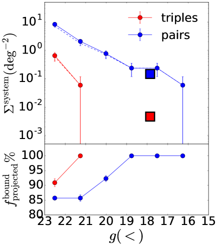
Figure 1: Top panels: Filled circles connected by solid lines show the surface density of simulated AGN projected pairs (blue) and triples (red) over $0.02\lesssim z\lesssim 0.15$ with $d^{\parallel}_{\mathrm{max}}=0.1~{}\mathrm{cMpc}/h$ and line of sight velocity difference of $600~{}\mathrm{km/sec}$. The dashed lines represent the surface densities of the subset of pairs (blue) and triples (red) satisfying the same foregoing criteria, but are also bound. The filled squares represent observed surface densities of pairs (blue) and triples (red) inferred from Liu et al. (2011b). Bottom panels: Percentage of the projected pairs and triples (plotted in top panel) that are bound. The error-bars correspond to Poisson errors of the number counts.

Before focusing on AGN triples and quadruples, we first look at abundances of projected AGN pairs at $\sim 100~{}\mathrm{ckpc}/h$ scales (the prefix ’$c$’ denotes that the distance is in comoving units), and compare them to constraints from SDSS (Liu et al., 2011b). In Figure 1, we show surface densities of projected AGN pairs and triples at $0.02\lesssim z\lesssim 0.15$, with selection criteria similar to that of Liu et al. (2011b) i.e. line of sight velocity differences of $600~{}\mathrm{kms/sec}$ and separations $\lesssim 0.1~{}\mathrm{Mpc}/h$ on the plane of sky. We obtain these surface densities by computing the volume densities (at each available snapshot between $z\sim 0.02$ and $z\sim 0.15$) and integrating them over $0.02\lesssim z\lesssim 0.15$ using Eq. 4. Filled circles in blue show abundances of pairs in MBII; these are compared to surface densities inferred from observed AGN pairs (blue square) in Liu et al. (2011b) derived from samples of obscured AGNs in SDSS-DR7 (Abazajian et al., 2009). We find that the abundances of projected pairs in MBII are broadly consistent with the observed AGN projected pairs. This agreement is despite the fact that the observed samples contain only obscured AGNs whereas the simulated sample includes both obscured and unobscured AGNs, however obscured AGNs have also been found to dominate the overall AGN population (Buchner et al., 2015). We also show the simulated and observed triples as red circles and squares respectively, but abundances of AGN triples with $g<21$ are too small to be probed by the simulation given its volume. The bottom panels in Figure 1 show that $\gtrsim~{}85\%$ percent of these projected pairs are bound at $g<23$. The percentage increases with increasing brightness and for $g\lesssim 19$, all projected pairs are bound; this implies that according to MBII, almost all projected pairs in Liu et al. (2011b) are expected to be bound. Furthermore, the percentages of bound pairs are significantly higher compared to those derived using criteria from Hennawi et al. (2006) (shown later in Figure 5). This is simply due to significantly smaller plane of sky separations and velocity differences adopted by Liu et al. (2011b) compared to Hennawi et al. (2006).

We have therefore established that the lowest order AGN systems (pairs) in MBII have abundances that are comparable to existing observations. This serves as a validation for our tool (MBII), and motivates us to proceed further and use it to look at the higher order AGN systems (triples/ quadruples).

3.2 At what scales are AGN systems gravitationally bound?

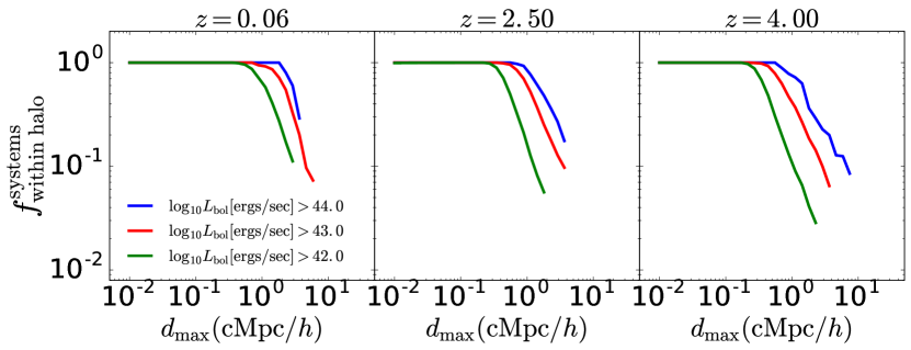
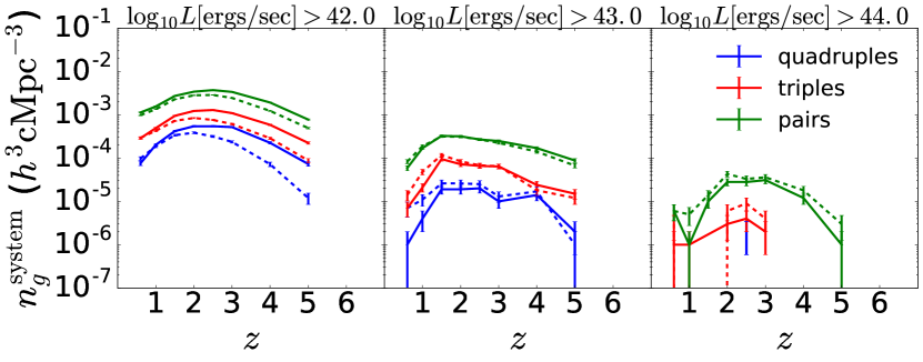
Figure 2: $f^{\mathrm{system}}_{\mathrm{within~{}halo}}$ is the fraction of physical AGN systems ($\texttt{RICHNESS}>1$) which are completely embedded within a common host halo, as a function of scale $d_{\mathrm{max}}$ defined as the maximum distance of separation between member AGNs.

Figure 3: Solid lines show the volume density of physical AGN systems (pairs, triples and quadruples at $d_{\mathrm{max}}=0.7~{}\mathrm{cMpc}/h$) as a function of redshift from $z=0.6$ to $z=5$. The dashed lines show the volume density of bound AGN systems (i.e. within the same FOF halo) over the desired redshift range. The errorbars correspond to Poisson errors in the number counts.

We now look at AGN systems (pairs, triples and beyond) for a wider range of scales ($\sim 10~{}\mathrm{ckpc}/h-10~{}\mathrm{cMpc}/h$) quantified by $d_{\mathrm{max}}$ (see Section 2.2). Our main objective is to prescribe a scale for targeting those physical AGN systems which are gravitationally bound (i.e. all members belong to the same FOF halo). Figure 3 shows the fraction ($f^{\mathrm{systems}}_{\mathrm{within~{}halo}}$) of physical AGN systems ($R>1$) completely embedded within a single host halo, as a function of scale $d_{\mathrm{max}}$ (note that we are considering physical AGN systems at length scales $\gtrsim 10~{}\mathrm{ckpc}/h$, which is roughly 10 times larger than the spatial resolution/ gravitational smoothing length of the simulation. We do this to minimize the possibility of our predictions to be affected by the finite spatial resolution of the simulation). Different panels show different redshifts ranging from $z\sim 0$ to $z\sim 4$ and different colors correspond to different luminosity cuts. At small enough scales, all the physical AGN systems are bound ($f^{\mathrm{systems}}_{\mathrm{within~{}halo}}\rightarrow 1$). Beyond a certain scale (which we will refer to as $d_{\mathrm{max}}^{0}$), physical AGN systems start to include members across different halos leading to a sharp drop in $f^{\mathrm{systems}}_{\mathrm{within~{}halo}}$ for $d_{\mathrm{max}}>d_{\mathrm{max}}^{0}$.

$d_{\mathrm{max}}^{0}$ depends on the typical sizes of haloes which host AGNs. The trends in Figure 3 show that $d_{\mathrm{max}}^{0}$ increases with luminosity at fixed redshift because more luminous AGNs live in more massive haloes (DeGraf & Sijacki, 2017; Bhowmick et al., 2019). Likewise, $d_{\mathrm{max}}^{0}$ decreases with increasing redshift (at fixed luminosity) because host haloes become smaller at higher redshift. Overall, $d_{\mathrm{max}}^{0}$ ranges from $\sim 0.5-2~{}\mathrm{cMpc}/h$ depending on the luminosity and redshift.

The foregoing motivates us to focus on $d_{\mathrm{max}}\sim 0.5-2~{}\mathrm{cMpc}/h$. For instance, in Figure 3 we select a value within this range, specifically $d_{\mathrm{max}}\sim 0.7~{}\mathrm{cMpc}/h$ to show the volume density of AGN systems. The solid lines show the volume density of physical AGN systems i.e. pairs, triples and quadruples ($R=2,3,4$) as a function of redshift. These can be compared to the dashed lines which represent bound AGN systems. The volume density of physical and bound systems are similar for $L_{\mathrm{bol}}>10^{43,44}~{}\mathrm{ergs/sec}$ AGNs. We therefore hereafter (unless stated otherwise) present results for $d_{\mathrm{max}}=0.7~{}\mathrm{cMpc}/h$; with this choice, we are primarily targeting physical AGN systems which are within the same halo (and are therefore bound). Note that our choice of scale is also comparable to the scales of observed AGN systems (Djorgovski et al., 2007; Myers et al., 2008; Farina et al., 2013; Hennawi et al., 2015).

We also see in Figure 3 that AGN systems are most abundant at the epoch $1.5\lesssim z\lesssim 3$. In this epoch, the volume density of AGN triples with $L_{\mathrm{bol}}>10^{44}~{}\mathrm{ergs/sec}$ (rightmost panel) is $\sim 10^{-6}~{}h^{3}\mathrm{cMpc}^{-3}$.

3.3 Dependence of AGN multiplicity function on $R$

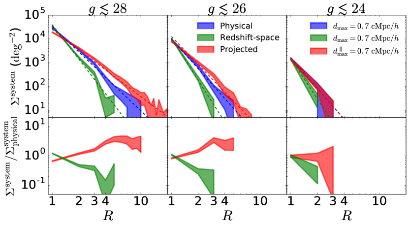
Figure 4: AGN multiplicity function:- Top panels: $\Sigma^{\mathrm{system}}$ is the surface density of physical, redshift space and projected ($v_{\mathrm{max}}=2000~{}\mathrm{km/sec}$) AGN systems between redshifts $0.06\lesssim z\lesssim 4$ plotted as a function of richness $\mathrm{R}$ (number of AGNs in a system) for different flux limits in the g-band. The middle and right panels roughly correspond to the expected flux limits of the LSST (LSST Science Collaboration et al., 2009) and DESI (DESI Collaboration et al., 2016) surveys respectively. Additionally, we also show (left panel) AGN systems 2 magnitudes fainter than the LSST limit at which MBII contains physical AGN systems with upto $\sim 10$ members. The dashed lines are best fit power-laws (coefficients are provided in Table 1). Bottom panels: Ratio of surface density of projected and redshift-space systems with respect to physical AGN systems as a function of $R$. The scatter corresponds to Poisson error.

$g(<)$	$\alpha$	$\Sigma_{1}$
	Physical
28	$-3.5$	$3.2\times 10^{4}$
26	$-4.1$	$1.0\times 10^{4}$
24	$-4.2$	$1.6\times 10^{3}$
	Redshift-space
28	$-4.8$	$4.0\times 10^{4}$
26	$-5.8$	$1.1\times 10^{4}$
24	$-5.6$	$1.4\times 10^{3}$
	Projected
28	$-2.8$	$2.5\times 10^{4}$
26	$-3.9$	$1.2\times 10^{4}$
24	$-4.2$	$1.5\times 10^{3}$

Table 1: Best fit values of power-law coefficients $\alpha$ and $\Sigma_{1}$ for various types of AGN systems. $g(<)$ is the threshold magnitude in the $g$ band. The power law fits are shown as dashed lines in Figure 4.

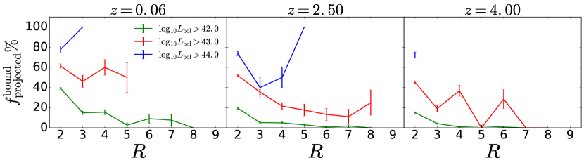
Figure 5: The percentage of the projected ($d^{\parallel}_{\mathrm{max}}=0.7~{}\mathrm{cMpc}/h$ and $v_{\mathrm{max}}=2000~{}\mathrm{km/sec}$) AGN systems that are bound (all members belong to the same host halo) versus richness. The errorbars correspond to Poisson errors in the number counts of projected systems and bound systems .

With $\sim 0.7~{}\mathrm{cMpc}/h$ identified as the target scale for gravitational bound AGN systems, we finally present the full multiplicity functions of MBII AGNs as a function of richness $R$. Figure 4 shows the surface density of AGN systems as a function of $R$. The g-band apparent magnitude limits have been chosen to be consistent with the expected detection limits of upcoming surveys such as DESI for $g<24$ (DESI Collaboration et al., 2016), LSST (LSST Science Collaboration et al., 2009) for $g<26$, and HST (Lallo, 2012) for $g<28$. $g<24$ is also representative of surveys such as JPASS (Benitez et al., 2014), SPHEREX (Doré et al., 2014) and PAU (Eriksen et al., 2019). Note that observationally, AGN systems are typically confirmed via spectroscopic follow-up, and spectroscopic surveys such as eBOSS (Dawson et al., 2016), DESI (and possible future follow-up to LSST) will be limited in their detectibility due to the fibre-collision limit. We shall discuss the effect of these limitations in Section 9. In this section, we will focus on the intrinsic abundance of AGN systems at various depths encompassing the imaging areas of HST, DESI (provided by the Legacy Surveys; see, e.g. Dey et al., 2018) and the LSST.

The surface densities in Figure 4 are calculated by integrating the volume density over redshifts ranging from $0.06\lesssim z\lesssim 4$ using Eq. (4). Blue, green and red shaded regions correspond to physical, redshift-space and projected AGN systems as defined in Section 2.2. For the physical and redshift-space systems we use $d_{\mathrm{max}}=0.7~{}\mathrm{cMpc}/h$ (representative of bound AGN systems as already discussed in Figure 3). For the projected systems, we use $d_{\mathrm{max}}^{\parallel}=0.7~{}\mathrm{cMpc}/h$ (maximum distance between members parallel to the plane of the sky). We find that the surface density of AGN systems exhibits a power-law decrease w.r.t increase in $R$. The power law may be described as

$$\Sigma^{\mathrm{system}}=\Sigma_{1}R^{\alpha}$$ (8)

where $\alpha$ is the power-law slope and $\Sigma_{1}$ is a coefficient measuring the number of isolated AGNs (i.e. $R=1$). The power-law fits are shown as dashed lines, and the values of $\alpha$ and $\Sigma_{1}$ are tabulated in Table 1. The exponents range from $\sim-3$ to $\sim-6$ depending on the type of system and the magnitude threshold. For instance, for projected AGN systems with $g<24,26$ we see that $\alpha\sim-4$, which implies that roughly $\sim 10\%$ of AGNs are part of AGN systems (pair or higher) with $d_{\mathrm{max}}^{\parallel}=0.7~{}\mathrm{cMpc}/h$. It is also worthwhile to note that if we reduce $d_{\mathrm{max}}^{\parallel}$ to $\sim 30~{}\mathrm{ckpc}/h$, only $\sim 1\%$ of AGNs are part of AGN systems (pair or higher), and this is consistent with predictions from EAGLE hydrodynamic simulation (Rosas-Guevara et al., 2019).

From the multiplicity functions, we can read off the abundances of triples/ quadruples at various depths. Let us first focus on the abundances of physical triples/ quadruples. At $g<24$ (depth of DESI imaging), surface density of available physical triples is $\sim 10$ per $\mathrm{deg}^{2}$. Likewise, at $g<26$ (depth of LSST imaging) MBII predicts $\sim 100$ physical triples/ quadruples per $\mathrm{deg}^{2}$. Lastly, at $g<28$ (depth of HST imaging), MBII predicts $\sim 700$ physical triples/ quadruples per $\mathrm{deg}^{2}$.

The comparison between the multiplicity functions for physical and redshift-space AGN systems is of particular interest because observations can only access the latter. We find that multiplicity functions for redshift-space AGN systems are significantly more suppressed (by factors up to $\sim 10$) compared to physical AGN systems. This occurs because of the dispersion in peculiar velocities of AGNs at small (one-halo) scales which leads to higher line of sight separations between member AGNs in redshift space as compared to real space. This implies that the sample of AGN systems obtained from a spectroscopic follow-up of projected AGNs may not include all possible physical/bound AGN systems. This can be corrected by simply choosing a larger line of sight (redshift space) separation $d_{\mathrm{max}}^{\perp}$ compared to $d_{\mathrm{max}}^{\parallel}$. We compare the multiplicity functions for physical and redshift-space systems for a wide range of ratios $d_{\mathrm{max}}^{\perp}/d_{\mathrm{max}}^{\parallel}$; we find that in order to match the multiplicity functions for redshift-space and physical AGN systems, we would require $d_{\mathrm{max}}^{\perp}/d_{\mathrm{max}}^{\parallel}\sim 5$. In other words, for $d_{\mathrm{max}}^{\perp}/d_{\mathrm{max}}^{\parallel}>5$ and $d_{\mathrm{max}}^{\parallel}\sim 0.7~{}\mathrm{Mpc}/h$, the chosen line of sight separation is too large causing the multiplicity functions to be contaminated by systems that are unbound. On the other hand, for $d_{\mathrm{max}}^{\perp}/d_{\mathrm{max}}^{\parallel}<5$ and $d_{\mathrm{max}}^{\parallel}\sim 0.7~{}\mathrm{Mpc}/h$, the chosen line of sight separation is too small, leading to significant number of bound systems that would be missed.

3.3.1 How to target gravitationally bound AGN systems in observations?

We now have all the information required to target bound AGN systems in observations. To ensure that the members are indeed bound (i.e. belonging to the same halo), the comoving separation should be $\lesssim 0.7~{}\mathrm{cMpc}/h$. This corresponds to maximum angular separations ranging from $\lesssim 100~{}\mathrm{arcsec}$ at $z\sim 0.6$ to $\lesssim 30~{}\mathrm{arcsec}$ at $z\sim 4$. Along the line of sight co-ordinate, $\lesssim 0.7~{}\mathrm{cMpc}/h$ corresponds to maximum spectroscopic redshift separations ranging from $\delta z\lesssim 5\times 10^{-4}$) at $z\sim 0.6$ to $\delta z\lesssim 1\times 10^{-3}$ at $z\sim 4$. However, to compensate for the broadening of the line of sight separations due to peculiar velocity dispersions, one must increase the line of sight separation by factors $\sim 5$, implying maximum spectroscopic redshift separations ranging from $\delta z\sim 1.5\times 10^{-3}$ at $z\sim 0.6$ to $\delta z\sim 7\times 10^{-3}$ at $z\sim 4$. The corresponding values of the maximum line of sight velocity difference range from $\lesssim 150~{}\mathrm{km/sec}$ at $z\sim 0.6$ to $\lesssim 200~{}\mathrm{km/sec}$ at $z\sim 4$. By applying the foregoing conditions, we can ensure that a spectroscopically confirmed sample of observed AGN systems shall correspond to a complete sample of bound AGN systems.

The inferred velocity separations for bound AGN systems is about 10 times smaller than the $2000~{}\mathrm{km/sec}$. This limit was adopted by Hennawi et al. (2006), which includes velocity differences up to $\sim 500~{}\mathrm{km/sec}$ expected from peculiar velocities, as well as the redshift uncertainties caused by blue-shifted broad lines (Richards et al., 2002) of the member AGNs. Therefore, not all projected systems are bound. We therefore naturally expect more projected AGN systems compared to physical/ redshift-space AGN systems, as clearly seen in Figure 4. The solid lines in Figure 5 show the percentage of projected ($v_{\mathrm{max}}=2000~{}\mathrm{km/sec}$, $d_{\mathrm{max}}=0.7~{}\mathrm{cMpc}/h$) systems that are bound. We see that for $L_{\mathrm{bol}}>10^{42}~{}\mathrm{ergs/sec}$ (solid blue line), $\sim 40\%$ and $\sim 20\%$ of AGN systems are bound at $z=0.06$ and $z=2.5$ respectively. We also see that at higher luminosities, a higher percentage of projected AGN systems are bound ($\sim 50\%$ for $L_{\mathrm{bol}}>10^{43}~{}\mathrm{ergs/sec}$). As a result, the difference between the multiplicity functions of physical and projected AGN systems decreases in Figure 4 with increasing brightness. This is expected because with increasing luminosity, AGNs becomes rarer, which results in a decreased likelihood of a chance superposition of otherwise unbound AGNs on a projected plane.

3.3.2 Predictions for $g<22$ (eBOSS depths) AGN systems using HOD modeling

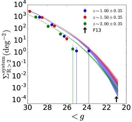
Figure 6: Surface density of physical AGN systems with $R>2$ (triples and higher-order systems) with $d_{\mathrm{max}}\sim 0.7~{}\mathrm{cMpc}/h$ (angular separations $\lesssim 50~{}\mathrm{arcsec}$) as a function of limiting $g$ band magnitude. The different colors correspond to different redshift bins within the target selection of eBOSS-CORE quasars, further limited to $0.9\lesssim z\lesssim 2.2$ where optical selection of quasars is most efficient. The shaded regions correspond to the predictions (upper limit) of a HOD model constrained by recent small-scale clustering measurements (Eftekharzadeh et al., 2017; Bhowmick et al., 2019). The black arrow is a lower limit inferred from the observation of an AGN triple in Farina et al. (2013).

MBII directly probes AGN triples/ quadruples up to $g\sim 24$ over $0.06\lesssim z\lesssim 4$. In order to reach eBOSS like depths ($g\sim 22$), we use the HOD model built in Bhowmick et al. (2019) (see Section 2.4 and Appendix A for more details) and make predictions beyond the simulated regime. These are shown as shaded regions in Figure 6. The black arrow corresponds to the lower limit inferred from the current state of observations i.e. 1 triple found (Farina et al., 2013) so far during the follow-up search in the sample from SDSS-DR6 (Richards et al., 2009). Our predictions therefore do not conflict with observations so far. For $g<22$ (the approximate depth eBOSS-CORE), we predict $\sim 10^{-2}$ systems per $\mathrm{deg}^{2}$, implying $\sim 100$ AGN triples (and higher-order systems) over the entire (imaging) area ($\sim 7500~{}\mathrm{deg}^{2}$) of eBOSS.

3.4 Effect of volume limit on multiplicity functions

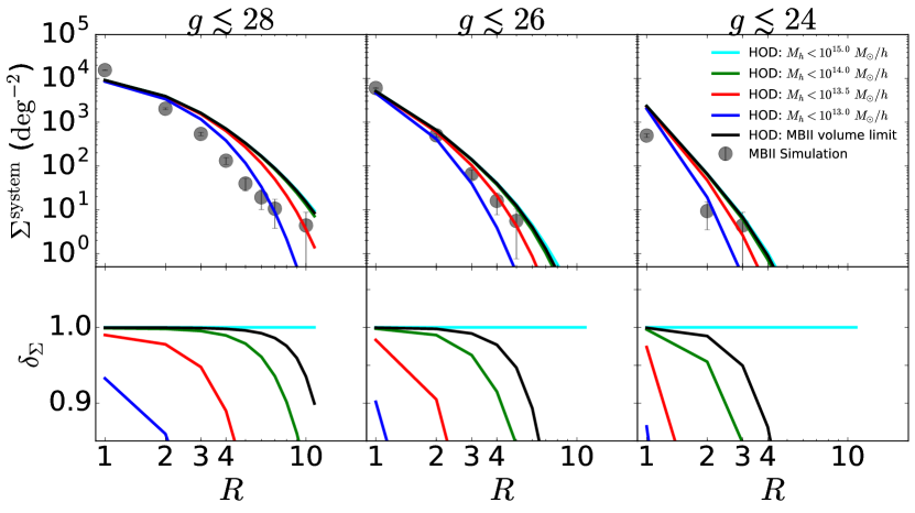
Figure 7: Top Panels: Solid lines show the HOD model predictions for the surface densities of bound AGN systems over $0.6\lesssim z\lesssim 2$. Different colors correspond to various upper limits in the halo mass in Eq. (7), representative of different simulation volumes. Filled circles are the simulation predictions with errorbars showing Poisson errors. Bottom Panels: $\delta_{\Sigma}$ is the ratio between HOD model multiplicity functions with respect to that of $M_{h}<10^{15}~{}M_{\odot}/h$.

The multiplicity functions in MBII can be potentially underestimated due to finite volume in the simulation, particularly for the AGN systems that are the brightest and have the highest richness. This is because the rarest massive haloes ($M_{H}\gtrsim 10^{14}~{}M_{\odot}/h$) are too rare to be captured by the simulation. This is typical of all hydrodynamic simulations, and at its resolution MBII is amongst the largest set of cosmological hydrodynamic simulations run till date.

In order to estimate the possible suppression due to the finite volume, we use HOD modelling, wherein we effectively populate central and satellite AGNs on the halo mass function of Tinker et al. (2008), which has been calibrated to $~{}5\%$ accuracy with N-body simulations over $10^{11}\lesssim M_{h}\lesssim 10^{15}~{}M_{\odot}/h$. As described in Section 2.4, HOD model was built using small scale clustering constraints at $0.6\lesssim z\lesssim 2$; we therefore select this redshift range to provide our estimate. We show in Figure 7: top panels HOD model predictions of the multiplicity functions (surface density) of bound AGN systems over $0.6\lesssim z\lesssim 2$. We have modelled the effect of finite volume as an upper limit of halo mass ($M_{h}(<)$) in the integral of Eq. (3). Solid lines (blue, green, red and cyan) show predictions for various possible volumes corresponding to $M_{h}(<)=10^{13,13.5,14,15}~{}M_{\odot}/h$. As expected, the differences amongst the solid lines become more pronounced at higher richness and brighter magnitudes. We see that the multiplicity functions converge when the upper limit is $M_{h}\sim 10^{15}~{}M_{\odot}/h$ (cyan line), with no significant contribution coming from higher mass ($M_{h}\gtrsim 10^{15}~{}M_{\odot}/h$) haloes. We now seek an HOD model prediction that is representative of the MBII volume. MBII (given its volume) can probe up to halo masses of $M_{h}\sim 6\times 10^{13},1\times 10^{14},2\times 10^{14},4\times 10^{14}~{}M_{\odot}/h$ at $z=2,1.5,1.0,0.6$ snapshots respectively. Accordingly, we choose these different upper limits at the respective redshifts to compute an HOD model prediction to the multiplicity function for the MBII volume over $0.6<z<2$. This is shown by the solid black line. Comparing the solid black line and the cyan line then provides an estimate of the suppression in the MBII multiplicity functions due to its finite volume. In the bottom panel of Figure 7 we show $\delta_{\Sigma}$, which is defined as the ratio of the HOD model multiplicity functions with respect to that of $M_{h}<10^{15}~{}M_{\odot}/h$. The black lines in the bottom panels correspond to the ratio between black and cyan lines of the top panel. They show that according to HOD modeling, the number of triples/ quadraples in MBII may be suppressed (due to finite volume) by factors of $\sim 0.85$, $0.97$, $\gtrsim 0.99$ for $g<24,26,28$ respectively. Overall, this implies that the finite simulation volume of MBII leads to a very marginal suppression ($\lesssim 15\%$) on the predictions of its multiplicity functions.

3.5 Effect of spectroscopic fibre collisions on the multiplicity functions

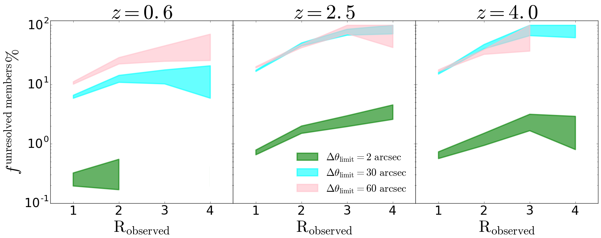
Figure 8: $f^{\mathrm{unresolved~{}members}}$ is the percentage of AGN systems with richness $R_{\mathrm{observed}}$ that have at least one other extra member unresolved due to fibre collisions. $\Delta\theta_{\mathrm{limit}}$ is the minimum angular separation between two adjacent fibres. The shaded region shows the Poisson error. This plot shows AGN systems with $L_{\mathrm{bol}}>10^{42}~{}\mathrm{ergs/sec}$.

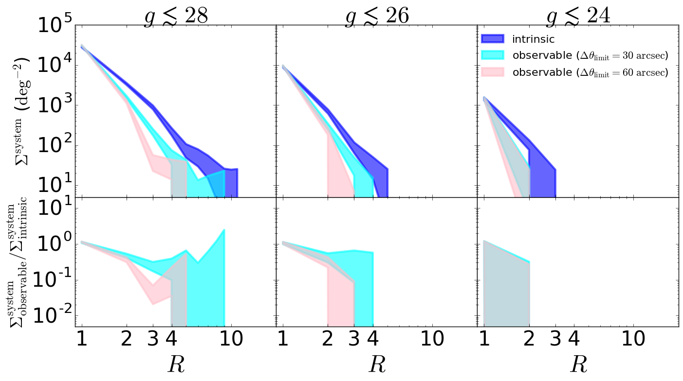
Figure 9: AGN multiplicity function with correction for fibre collisions:- Top panels: $\Sigma^{\mathrm{system}}$ is the surface density of AGN systems ($d_{\mathrm{max}}=0.7~{}\mathrm{cMpc}/h$) over redshifts $0.06\lesssim z\lesssim 4$, plotted as a function of richness $\mathrm{R}$. The scatter corresponds to $1\sigma$ Poisson error. The blue region ($\Sigma^{\mathrm{system}}_{\mathrm{intrinsic}}$) corresponds to the intrinsic abundance of physical AGN systems as also shown in Figure 4. The cyan and pink regions ($\Sigma^{\mathrm{system}}_{\mathrm{observable}}$) correspond to observed abundances of AGN systems in the presence of a fibre-collision limit $\Delta\theta_{\mathrm{limit}}$ (see section 9). We assume a $30\%$ overlap between the areas of adjacent tiles. Bottom panels: Ratio between $\Sigma^{\mathrm{system}}_{\mathrm{observable}}$ and $\Sigma^{\mathrm{system}}_{\mathrm{intrinsic}}$.

As mentioned in Section 3.3, detectable AGN systems in spectroscopic surveys are subject to a minimum angular separation due to the fibre collision limit i.e. the minimum distance between adjacent fibres on a single spectroscopic tile (see, e.g. Blanton et al., 2003, for details on tiling algorithms). Here, we study its implications on the inferred multiplicity functions. We consider the following two crucial effects in our modeling.

• Loss of member AGNs due to spectroscopic fibre collisions: To model this, we define a minimum angular separation, $\Delta\theta_{\mathrm{limit}}$ (hereafter referred as the fibre collision limit), such that member AGNs at smaller separations cannot be distinguished from one another. We consider fibre collision limit of $60~{}\mathrm{arcsec}$, roughly representative of the SDSS, BOSS and eBOSS technical specifications (Blanton et al., 2003; Dawson et al., 2013, 2016). Additionally, we also consider fibre collision limit of $30~{}\mathrm{arcsec}$, roughly consistent with a lower bound for DESI (this will however depend on exactly how the DESI focal plane is populated).

• Recovery of member AGNs in regions with overlapping tiles: We assume $30\%$ overlap between surface areas of neighboring tiles, roughly representative of the layout of the tiles in the SDSS survey (Blanton et al., 2003). A pair of AGNs in an area covered by overlapping tiles can be distinguished from one another despite having angular separations of less than $\Delta\theta_{\mathrm{limit}}$. Note, however, that our chosen $30\%$ overlap is a gross simplification for the DESI survey, for which the planned layout of tiles is quite complex, with multiple layers of spectroscopic tiles (see Section 4 of DESI Collaboration et al., 2016).

Specifically, we consider each physical AGN system with original richness $R$ and $d_{\mathrm{max}}=0.7~{}\mathrm{cMpc}/h$ (shaded blue region in Figure 4), calculate angular separations between their members, and reduce their richness by 1 unit for every distinct pair of members with angular separations below the resolution. We then randomly choose $30\%$ of the overlapping pairs and recover them i.e. for each of the recovered pair, we increase the richness of the parent system by 1 unit. We refer to the resulting richness of the system as $R_{\mathrm{observed}}$. $R_{\mathrm{observed}}$ is inevitably less than or equal to intrinsic richness $R$.

Figure 8 shows the percentage ($f^{\mathrm{unresolved\ members}}~{}\%$) of AGN systems ($L_{\mathrm{bol}}>10^{42}~{}\mathrm{ergs/sec}$) with at least one extra unresolved member, for fibre collision limits of $30~{}\mathrm{arcsec}$ (cyan region) and $60~{}\mathrm{arcsec}$ (pink region). We see that about $\sim 10\%$ of observed single AGNs at $z=0.6$ (leftmost panel) have unresolved members, which increases to $\sim 20\%$ at $z=2.5,4$ (middle and rightmost panels); this is expected as the fibre collision limit ($\Delta\theta_{\mathrm{limit}}$) subtends a larger comoving separation at higher redshifts, leading to higher number of unresolved members. Additionally, we also see that higher the observed richness of a system, higher the probability of the system having additional unresolved members. For instance, at fibre collision limit of $30~{}\mathrm{arcsec}$, observed AGN triples and quadruples at $z=2.5$ and $z=4$ have $\gtrsim 60\%$ chance of revealing additional unresolved members upon a possible future follow-up spectroscopic survey with lower fibre collision limit. In addition to the fibre collision limits of $30-60$ arcsec, it is also instructive to show $\Delta\theta_{\mathrm{limit}}=2~{}\mathrm{arcsec}$ (green region in Figure 8). This is representative of angular resolution limits due to the point spread function (PSF) of an observed source, and corresponds to $\lesssim 70~{}\mathrm{ckpc}$ at $z<4$. We see that at $z=2.5,4$, about $\sim 1-3\%$ of systems contain additional unresolved members; at $z=0.6$, only about $\sim 0.3\%$ of systems contain additional unresolved members. Therefore the percentage ($f^{\mathrm{unresolved\ members}}~{}\%$) for the PSF limit of 2 arcsec is negligibly small compared to that of the fibre collision limits of $30-60~{}\mathrm{arcsec}$. Overall, this implies that the impact of the PSF limit on our inferred multiplicity functions for $d_{\mathrm{max}}=0.7~{}\mathrm{cMpc}/h$ is not very significant. In the next paragraph, we address the impact of the fibre collision limits on the multiplicity functions.

Figure 9 shows the impact of spectroscopic fibre collisions on the inferred multiplicity function. In the top panels, the blue region shows the intrinsic multiplicity function ($\Sigma^{\mathrm{system}}_{\mathrm{intrinsic}}$) of physical AGN systems (as in Figure 4); the cyan and pink regions show the multiplicity functions ($\Sigma^{\mathrm{system}}_{\mathrm{observable}}$) of the same set of AGN systems when corrected for fibre collision limits of $30~{}\mathrm{arcsec}$ and $60~{}\mathrm{arcsec}$ respectively. As expected, we see that with increasing $\Delta\theta_{\mathrm{limit}}$, we start to lose member AGNs and the abundance of higher order systems starts to get suppressed, leading to increasingly steep multiplicity functions. The bottom panels show the ratio between the observed multiplicity function and the intrinsic multiplicity function. We find that a fibre collision limit of $60~{}\mathrm{arcsec}$ suppresses the observed number of AGN triples/ quadruples by factors $\lesssim 0.2$); this implies that $\lesssim 20~{}\%$ of all available triples/quadruples are expected to be detected after spectroscopic follow-up. Note also that in regions with overlaps across multiple surveys such as SDSS and/or eBOSS and/or DESI, more missing members can be recovered. We do not model this effect as MBII does not directly probe AGN systems with magnitudes brighter than the SDSS and eBOSS detection limits (e.g., see Figure 6).

4 Origin and Environment of Quasar systems in MBII:

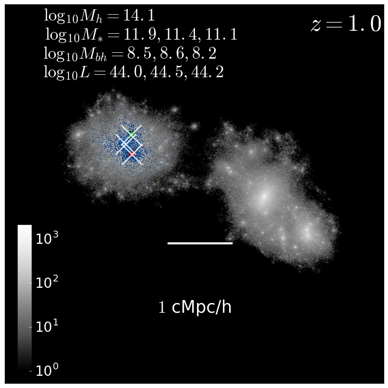
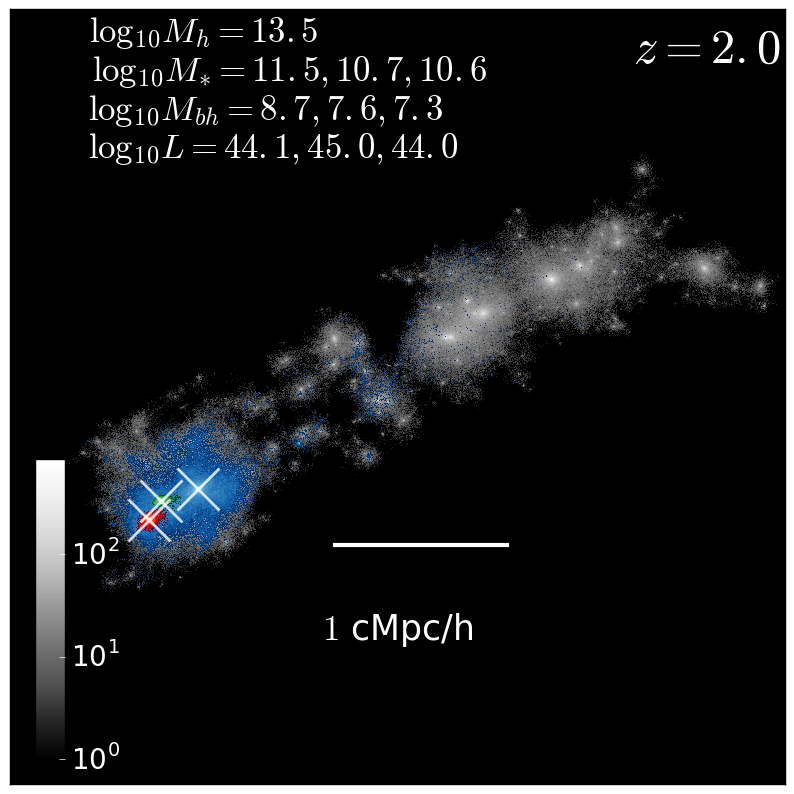
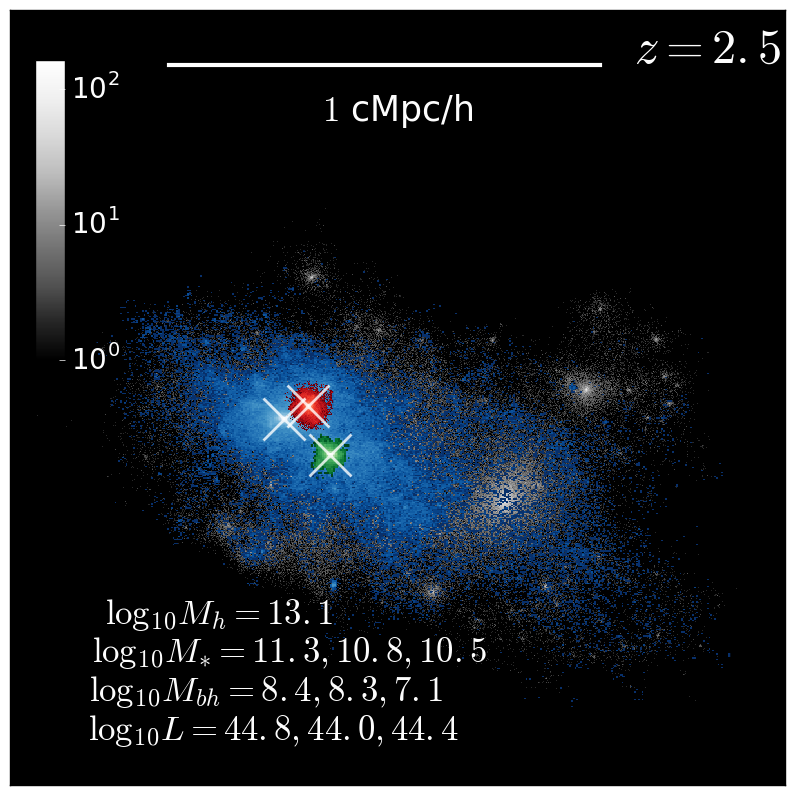
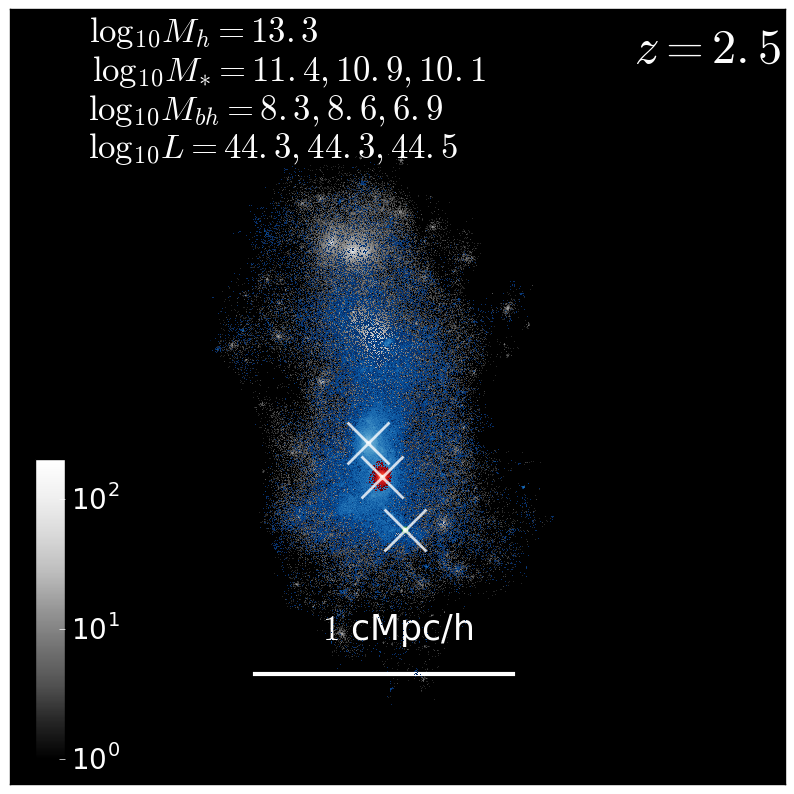
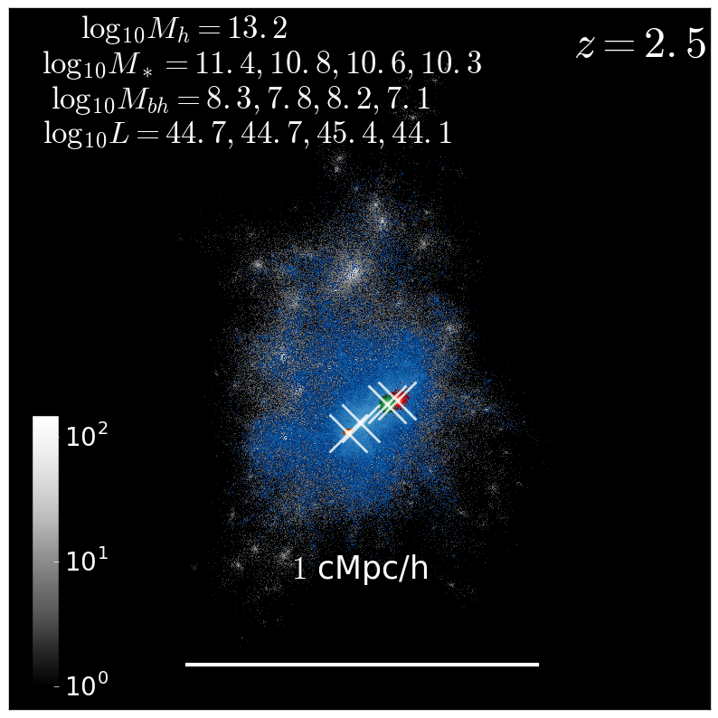
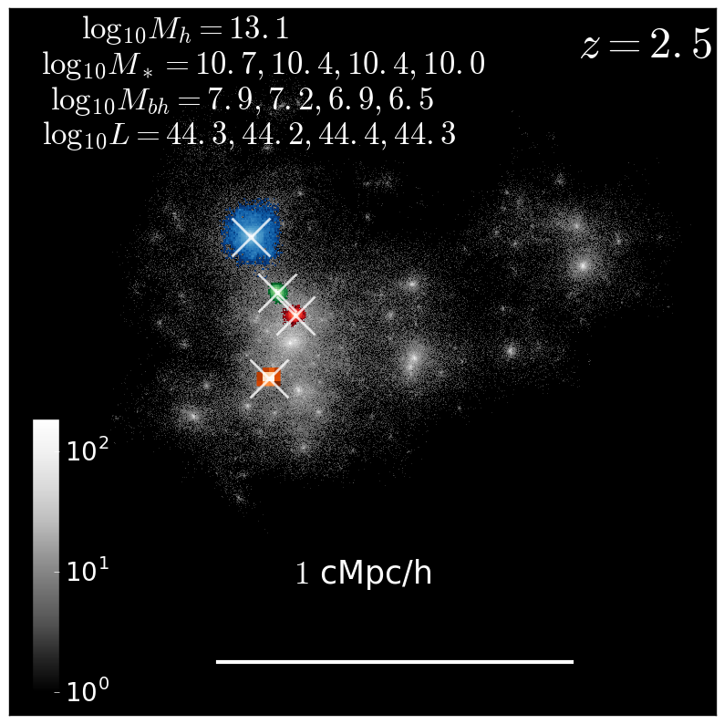
Figure 10: The crosses indicate the 2D projected positions of the simulated quasar triples and quadruples with $d_{\mathrm{max}}=0.7~{}\mathrm{cMpc}/h$ and $L_{\mathrm{bol}}>10^{44}~{}\mathrm{ergs/sec}$. Grey 2-D density histograms represent the host dark matter haloes and colored histograms depict the host galaxies. The blue histogram corresponds to the central galaxy and the red, green, and orange histograms represent the satellite galaxies. Consult the legend for the various properties of the quasars and their hosts. $M_{h}$, $M_{*}$ and $M_{bh}$ are halo masses, stellar masses and black-hole masses in units of $M_{\odot}/h$. $L$ is the bolometric luminosity in the units of $\mathrm{ergs/sec}$. The horizontal white line represents a length scale of $1~{}\mathrm{cMpc}/h$.

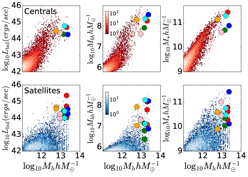
Figure 11: Filled circles show the host halo masses, host galaxy masses, black hole masses and luminosities of various quasar triples and quadruples with $L_{\mathrm{bol}}>10^{44}~{}\mathrm{ergs/sec}$ and $d_{\mathrm{max}}=0.7~{}\mathrm{cMpc}/h$ identified at $z=2.5$. The underlying histograms show the scaling relations between these properties for the overall AGN population at $z=2.5$. The blue histograms show satellite AGNs and red histograms show central AGNs.

Until now, we have focused on the abundances of AGN systems. Hereafter, we shall investigate the physical properties and environment of the most luminous AGN (quasar) systems in MBII. We will also study the growth histories of quasar systems to elucidate the physical mechanisms involved in their formation.

We focus on systems where each member has a luminosity $L_{\mathrm{bol}}>10^{44}~{}\mathrm{ergs/sec}$. Figure 10 shows images of these systems, along with their host galaxies (colored histograms) and host haloes (shown as grey histograms). The host halo masses for the systems are $\sim 10^{13}~{}M_{\odot}/h$. We note that these are amongst the most massive haloes in the simulation at the corresponding redshifts, in support of observational inferences (Farina et al., 2013; Hennawi et al., 2015) about these systems being progenitors of massive clusters; this is also consistently true for the simulated triples at $z=2$ and $z=1$, which live in $\sim 10^{13.5}~{}M_{\odot}/h$ and $\sim 10^{14}~{}M_{\odot}/h$ haloes respectively. Figure 10 shows that these systems have a very rich substructure i.e. a number of locally dense regions and complex morphologies, indicating possible occurrence of recent mergers. Within a halo, the member quasars live in different host galaxies (there are no $L_{\mathrm{bol}}>10^{44}~{}\mathrm{ergs/sec}$ quasar systems in MBII within the same galaxy). In particular, one member is hosted by the central (most massive) galaxy, and the other members are hosted by satellite galaxies. The central galaxies are illustrated in Figure 10 as blue histograms. The satellite galaxies are illustrated as red, green and orange histograms. The host galaxies have stellar masses in the range $10^{10}~{}\lesssim M_{*}\lesssim~{}10^{12}~{}M_{\odot}/h$. Their black hole masses range from $\sim 10^{6.5}$ to $\sim 10^{9}~{}M_{\odot}/h$.

Figure 11 shows the relationship of the various AGN properties (bolometric luminosity, black hole mass and host galaxy stellar mass) as a function of the host halo mass at $z=2.5$. The filled circles correspond to the quasar systems whereas the histograms show the overall population of simulated AGNs. The top and bottom panels correspond to central and satellite AGNs respectively. Circles of the same color correspond to the central (top panels) and satellite (bottom panels) member quasars within the same system. In the AGN luminosity vs. halo mass plane (lower-left panel of Figure 11), we can see that the satellite quasars have luminosities $\gtrsim 10-100$ times higher than the typical population of satellite AGNs residing in the respective host haloes ($M_{h}\gtrsim 10^{13}~{}M_{\odot}/h$). The black-hole mass vs. halo mass plane (lower-middle panel) shows that a handful of satellite quasars also have black hole masses $\gtrsim 10-100$ times higher than a typical satellite. However, the stellar mass vs. halo mass plane (lower right panel) shows that the host galaxies are more or less representative of the typical population of satellite AGN hosts. Overall, this hints at the possibility that the satellite quasars experienced a recent increase in their AGN activity. In the next subsection, we shall look at the growth histories of these AGNs and demonstrate that the increase in activity amongst satellite AGNs can be explained by recent major mergers amongst their progenitor host haloes.

4.1 Growth Histories

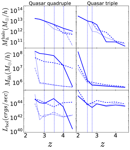
Figure 12: Growth history of an example quasar quadruple (left panels) and triple (right panels) shown in Figure 10. The panels from top to bottom correspond to the host halo mass, black hole mass and bolometric luminosity of the AGNs. The different line styles correspond to the different members of the system. Vertical lines of corresponding color show the time steps at which mergers of the host haloes occurred.

We now study the growth histories of the simulated triples and quadruples. Figure 12 shows the growth history of an example triple (right panel) and quadruple (left panel). The different line styles (solid, dashed, dot-dashed and dotted) correspond to different members of the system. The lowest redshift plotted for each line corresponds to the snapshot at which the objects form quasar systems with $L_{\mathrm{bol}}>10^{44}~{}\mathrm{ergs/sec}$.

Let us first focus on the quadruple (left-hand panel). The halo mass evolution (top panel) shows that the progenitors start out in four different haloes that experience a sequence of three mergers between $z=4$ and $z=2.5$ (shown as dotted vertical lines). Each merger is followed by an increase in AGN activity amongst one or both of the participating progenitors. For example, for the dotted line, the merger occured at $z=2.75$ after which the luminosity increased from $L_{\mathrm{bol}}<10^{42}~{}\mathrm{ergs/sec}$ at $z=2.75$ to $L_{\mathrm{bol}}>10^{45}~{}\mathrm{ergs/sec}$ at $z=2.5$. Concurrently, the black hole mass increased from $M_{bh}\lesssim 10^{6}~{}M_{\odot}/h$ at $z=2.75$ to $M_{bh}\gtrsim 10^{8}~{}M_{\odot}/h$ at $z=2.5$.

We report similar conclusions for the growth history of the triples (right panel of Figure 12 shows an example). The formation of each triple is associated with a sequence of two mergers of the host haloes of progenitor AGNs. These mergers triggered AGN activity to switch on the ‘quasar’ mode of the AGNs residing in these merging haloes.

While Figure 12 shows only a couple of examples of quasar triples/ quadruples, our findings are true for all the systems shown in Figure 10. In other words, all the multiple-quasar-systems in MBII originated from a sequence of multiple major mergers. These mergers not only bring together already active quasars, but also served as triggers of AGN activity transforming faint AGNs into luminous ($L>10^{44}~{}\mathrm{ergs/sec}$) quasars. Within MBII, we identified 5 members belonging to triple/ quadruple systems which were converted from faint AGNs ($L<10^{42}~{}\mathrm{ergs/sec}$) into luminous quasars ($L>10^{44}~{}\mathrm{ergs/sec}$) after a major merger. This merger driven activity was crucial to the formation of the quasar triples and quadruples. In fact, significant observational evidence of enhanced AGN activity in merged systems have also been reported in the last decade (Liu et al., 2011b; Silverman et al., 2011; Ellison et al., 2011, 2013; Lackner et al., 2014; Satyapal et al., 2014; Weston et al., 2017; Goulding et al., 2018; Ellison et al., 2019). Furthermore, we see that for all the simulated systems, haloes which merge belong to the rare massive end of the halo mass function at the corresponding redshift. In our previous paper (Bhowmick et al., 2019), we showed that bright quasar pairs originate from mergers of rare massive haloes. Here, we further show that in order to form richer quasar systems such as quasar triples, quadruples etc., we require a multiple sequence (more than one) of mergers of rare massive haloes. These events are exceptionally infrequent, explaining the sparsity of these quasar systems.

5 Conclusions and Future work

In this work, we have studied systems of AGNs at $0\lesssim z\lesssim 4$ and determine AGN multiplicity functions within the MBII simulation. We identified AGN systems at different scales by linking together AGNs within a certain distance. We find that to target gravitationally bound (within the same halo) AGN systems in observations, the maximum comoving distance between member AGNs should be $\sim 0.7~{}\mathrm{cMpc}/h$; this corresponds to maximum angular separations ranging from $\lesssim 100~{}\mathrm{arcsec}$ at $z\sim 0.6$ to $\lesssim 30~{}\mathrm{arcsec}$ at $z\sim 4$. Along the line of sight this corresponds to maximum velocity differences ranging from $\lesssim 150~{}\mathrm{km/sec}$ at $z\sim 0.6$ to $\lesssim 200~{}\mathrm{km/sec}$ at $z\sim 4$.

The multiplicity functions and their redshift evolution reveal that AGN systems (pairs, triples, quadruples) in MBII are most abundant at $1.5\lesssim z\lesssim 2.5$ wherein there are $10^{-5}$- $10^{-6}~{}h^{3}\mathrm{Mpc^{-3}}$ quasar triples with $L_{\mathrm{bol}}\gtrsim 10^{44}~{}\mathrm{ergs/sec}$. We find that the dependence of the multiplicity function as a function of $R$ can be well described by a power law with exponents ranging from $-3$ to $-6$. MBII directly probes AGN systems with magnitudes up to $g\sim 24$ at $0.06\lesssim z\lesssim 4$. We predict abundances of  10 triples or quadruples per $\mathrm{deg}^{2}$ at $g<24$ (depth of DESI imaging) and  100 triples or quadruples per $\mathrm{deg}^{2}$ at $g<26$ (depth of LSST imaging). To make predictions for $g<22$ (depth of eBOSS-CORE), we used HOD modeling; we predict a few $\times 10^{-2}~{}\mathrm{deg}^{-2}$ AGN triples/quadruples at $0.9\lesssim z\lesssim 2.2$. Using a simple model to describe fiber collisions, we predict that $\sim 20\%$ of the available triples or quadruples should be detectable after spectroscopic follow-up.

Finally, in order to probe the possible physical origins of these systems, we select a few of the most luminous ($L_{\mathrm{bol}}>10^{44}~{}\mathrm{ergs/sec}$) quasar triples and quadruples and study their environmental properties and growth histories. We find that their host haloes are amongst the most massive in the simulation ($\sim 10^{13}~{}M_{\odot}/h$ at $z=2.5$ and $\sim 10^{14}~{}M_{\odot}/h$ at $z=1$). Within these haloes, the members of quasar triples and quadruples always reside in separate galaxies, implying that one quasar lives in a central galaxy and the remaining quasars live in satellite galaxies. Note however that the simulations tend to assume instantaneous merger between black holes; a more accurate modeling of black hole mergers will likely lead to higher number of AGN systems living within the same host galaxy. Such models will therefore also lead to enhanced multiplicity functions particularly at small ($\lesssim 1~{}\mathrm{kpc}$) distances of separation. Furthermore, the gravitational recoil resulting from the merging process will influence the time evolution of the pair distances, and therefore may have a significant impact on the multiplicity functions. Future work shall investigate these aspects in detail. The galaxies have stellar masses $10^{10}\lesssim M_{*}\lesssim 10^{12}~{}M_{\odot}/h$ and black hole masses $10^{6}\lesssim M_{*}\lesssim 10^{9}~{}M_{\odot}/h$. Growth histories of these systems reveal that they were born out of a series of mergers (two mergers for triples and three mergers for quadruples) between rare massive haloes. These mergers can not only produce close pairs from already active quasars, but can also trigger significant activity in low-luminosity AGNs, transforming them into luminous quasars. This explains the wide range of black hole massses ($10^{6.5}\lesssim M_{bh}\lesssim 10^{9}~{}M_{\odot}/h$) for these objects. Sequences of multiple (two or more) mergers between the most massive haloes are exceedingly uncommon, explaining why these quasar systems are so rare.

Future work(s) can include investigations of further limitations in the detectibility of these AGN systems in observations. For instance, the member AGNs of these systems will have variability and are not always active; it is therefore important to determine how much this will reduce the probability of simultaneous detection of all the members of the system, and its impact on the observed multiplicity functions. Other avenues include an investigation of the effect of black hole seed models on the multiplicity functions, as well as predictions of gravitational wave signals sourced from such systems.

Appendix A Modeling of AGN HODs using Conditional Luminosity Function (CLF) formalism

We use AGN HODs which were derived in our previous work (Bhowmick et al., 2019) from small scale clustering constraints (Eftekharzadeh et al., 2017) at $0.6\lesssim z\lesssim 2$. In particular, we used the Conditional Luminosity function (CLF) model (Cooray, 2006) to parametrize the HODs. Under this model, for a given sample of AGNs with a luminosity threshold $L_{\mathrm{min}}$, the first order moment $\left<N(L>L_{\mathrm{min}},M_{h})\right>$ is given by

$$\left<N(L>L_{\mathrm{min}},M_{h})\right>=\int_{L_{\mathrm{min}}}^{\infty}~{}\tilde{\Phi}(L^{\prime},M_{h})~{}d\log_{10}L^{\prime}$$ (9)

where $\tilde{\Phi}(L,M_{h})$ is the Conditional luminosity function (CLF) defined as the distribution of AGN bolometric luminosities within haloes of masses $M_{h}$ to $M_{h}+dM_{h}$, such that

$$\int~{}\tilde{\Phi}(L,M_{h})~{}\frac{dn}{dM_{h}}~{}dM_{h}=\Phi(L)$$ (10)

where $\Phi(L)$ is the total quasar bolometric luminosity function.

The CLF can be separated into contributions from centrals ($\tilde{\Phi}_{\mathrm{cen}}(L,M_{h})$) and satellites ($\tilde{\Phi}_{\mathrm{sat}}(L,M_{h})$)

$$\tilde{\Phi}(L,M_{h})=\tilde{\Phi}_{\mathrm{cen}}(L,M_{h})+\tilde{\Phi}_{\mathrm{sat}}(L,M_{h}).$$ (11)

The CLF for central quasars can be parametrized as a log normal distribution

$$\tilde{\Phi}_{\mathrm{cen}}(L,M_{h})=Q_{\mathrm{cen}}~{}\frac{1}{2\pi\sigma_{\mathrm{cen}}}\exp{\left(-\frac{(\log_{10}{L}-\log_{10}{L^{*}_{\mathrm{cen}}})^{2}}{\sigma_{\mathrm{cen}}^{2}}\right)},$$

where $L^{*}_{\mathrm{cen}}$ is the average central AGN luminosity, $\sigma_{\mathrm{cen}}$ is the width of the log-normal distribution. $Q_{\mathrm{cen}}$ is the normalization of the central AGN. The CLFs for satellite quasars can be parametrized as a Schechter distribution

$$\tilde{\Phi}_{\mathrm{sat}}(L,M_{h})=Q_{\mathrm{sat}}\left(\frac{L}{L^{*}_{\mathrm{sat}}}\right)^{\alpha_{\mathrm{sat}}}\exp{\left(-\frac{L}{L^{*}_{\mathrm{sat}}}\right)}$$

$L^{*}_{\mathrm{sat}}$ measures the most luminous satellite for a given halo of mass $M_{h}$, $\alpha_{\mathrm{sat}}$ is the faint end slope of the distribution, and $Q_{\mathrm{sat}}$ is the normalization.

In Bhowmick et al. (2019), we used the simulation predictions and observed measurements of the luminosity function and the small scale clustering to constrain the parameters $Q_{\mathrm{cen}},\sigma_{\mathrm{cen}},L^{*}_{\mathrm{cen}},Q_{\mathrm{sat}},\alpha_{\mathrm{sat}},L^{*}_{\mathrm{sat}}$ to determine $\tilde{\Phi}(L,M_{h})$. We then used Eq. 9 to finally obtain the 1st order moments $\left<N\right>$ of central and satellite AGN HODs. Figure 13 shows the 1st order moments of the resulting mean occupations of central and satellite AGNs at $z=0.6,1,1.5,2$. In order to arrive the HODs ($P(N|M_{h})$ as defined in Section 2.4) from these moments, the satellite occupations are assumed to be Poisson. From $P(N|M_{h})$, one can then derive the multiplicity function using Eqs. (4-7).

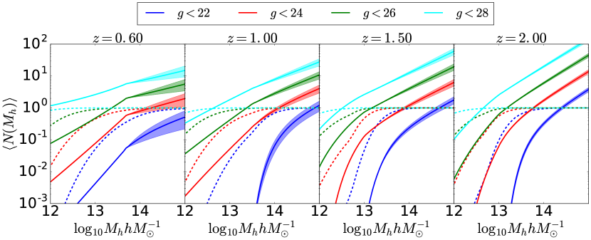
Figure 13: Mean occupations of satellite (solid lines) and central AGNs (dashed lines) as a function of halo mass over a redshift range of $0.6\lesssim z\lesssim 2$. The shaded regions correspond to uncertainties in the small scale ($\sim 25~{}\mathrm{kpc}/h$ ) clustering constraints in Eftekharzadeh et al. (2017).

References

- Abazajian et al. (2009) Abazajian K. N., et al., 2009, ApJS, 182, 543
- Babak et al. (2017) Babak S., et al., 2017, Phys. Rev. D, 95, 103012
- Benitez et al. (2014) Benitez N., et al., 2014, arXiv e-prints, p. arXiv:1403.5237
- Bhowmick et al. (2018) Bhowmick A. K., Campbell D., Di Matteo T., Feng Y., 2018, MNRAS, 480, 3177
- Bhowmick et al. (2019) Bhowmick A. K., DiMatteo T., Eftekharzadeh S., Myers A. D., 2019, MNRAS, 485, 2026
- Blanton et al. (2003) Blanton M. R., Lin H., Lupton R. H., Maley F. M., Young N., Zehavi I., Loveday J., 2003, AJ, 125, 2276
- Buchner et al. (2015) Buchner J., et al., 2015, ApJ, 802, 89
- Cooray (2006) Cooray A., 2006, MNRAS, 365, 842
- Croom et al. (2009) Croom S. M., et al., 2009, MNRAS, 399, 1755
- DESI Collaboration et al. (2016) DESI Collaboration et al., 2016, arXiv e-prints, p. arXiv:1611.00036
- Davis et al. (1985) Davis M., Efstathiou G., Frenk C. S., White S. D. M., 1985, ApJ, 292, 371
- Dawson et al. (2013) Dawson K. S., et al., 2013, AJ, 145, 10
- Dawson et al. (2016) Dawson K. S., et al., 2016, AJ, 151, 44
- DeGraf & Sijacki (2017) DeGraf C., Sijacki D., 2017, MNRAS, 466, 3331
- Dey et al. (2018) Dey A., et al., 2018, arXiv e-prints,
- Di Matteo et al. (2005) Di Matteo T., Springel V., Hernquist L., 2005, Nature, 433, 604
- Di Matteo et al. (2012) Di Matteo T., Khandai N., DeGraf C., Feng Y., Croft R. A. C., Lopez J., Springel V., 2012, ApJ, 745, L29
- Djorgovski et al. (2007) Djorgovski S. G., Courbin F., Meylan G., Sluse D., Thompson D., Mahabal A., Glikman E., 2007, ApJ, 662, L1
- Doré et al. (2014) Doré O., et al., 2014, arXiv e-prints, p. arXiv:1412.4872
- Eftekharzadeh et al. (2017) Eftekharzadeh S., Myers A. D., Hennawi J. F., Djorgovski S. G., Richards G. T., Mahabal A. A., Graham M. J., 2017, MNRAS, 468, 77
- Ellison et al. (2011) Ellison S. L., Patton D. R., Mendel J. T., Scudder J. M., 2011, MNRAS, 418, 2043
- Ellison et al. (2013) Ellison S. L., Mendel J. T., Patton D. R., Scudder J. M., 2013, MNRAS, 435, 3627
- Ellison et al. (2019) Ellison S. L., Viswanathan A., Patton D. R., Bottrell C., McConnachie A. W., Gwyn S., Cuillandre J.-C., 2019, MNRAS, 487, 2491
- Eriksen et al. (2019) Eriksen M., et al., 2019, MNRAS, 484, 4200
- Farina et al. (2013) Farina E. P., Montuori C., Decarli R., Fumagalli M., 2013, MNRAS, 431, 1019
- Goulding et al. (2018) Goulding A. D., et al., 2018, PASJ, 70, S37
- Hennawi et al. (2006) Hennawi J. F., et al., 2006, AJ, 131, 1
- Hennawi et al. (2015) Hennawi J. F., Prochaska J. X., Cantalupo S., Arrigoni-Battaia F., 2015, Science, 348, 779
- Kayo & Oguri (2012) Kayo I., Oguri M., 2012, MNRAS, 424, 1363
- Khandai et al. (2015) Khandai N., Di Matteo T., Croft R., Wilkins S., Feng Y., Tucker E., DeGraf C., Liu M.-S., 2015, MNRAS, 450, 1349
- Komatsu et al. (2011) Komatsu E., et al., 2011, ApJS, 192, 18
- LSST Science Collaboration et al. (2009) LSST Science Collaboration et al., 2009, arXiv e-prints, p. arXiv:0912.0201
- Lackner et al. (2014) Lackner C. N., et al., 2014, AJ, 148, 137
- Lallo (2012) Lallo M. D., 2012, Optical Engineering, 51, 011011
- Liu et al. (2011a) Liu X., Shen Y., Strauss M. A., 2011a, ApJ, 736, L7
- Liu et al. (2011b) Liu X., Shen Y., Strauss M. A., Hao L., 2011b, ApJ, 737, 101
- Liu et al. (2019) Liu X., et al., 2019, arXiv e-prints, p. arXiv:1907.10639
- McGreer et al. (2013) McGreer I. D., et al., 2013, ApJ, 768, 105
- McGreer et al. (2016) McGreer I. D., Eftekharzadeh S., Myers A. D., Fan X., 2016, AJ, 151, 61
- Myers et al. (2007) Myers A. D., Brunner R. J., Richards G. T., Nichol R. C., Schneider D. P., Bahcall N. A., 2007, ApJ, 658, 99
- Myers et al. (2008) Myers A. D., Richards G. T., Brunner R. J., Schneider D. P., Strand N. E., Hall P. B., Blomquist J. A., York D. G., 2008, ApJ, 678, 635
- Oke et al. (1995) Oke J. B., et al., 1995, PASP, 107, 375
- Palanque-Delabrouille et al. (2016) Palanque-Delabrouille N., et al., 2016, A&A, 587, A41
- Richards et al. (2002) Richards G. T., Vanden Berk D. E., Reichard T. A., Hall P. B., Schneider D. P., SubbaRao M., Thakar A. R., York D. G., 2002, AJ, 124, 1
- Richards et al. (2009) Richards G. T., et al., 2009, ApJS, 180, 67
- Rosas-Guevara et al. (2019) Rosas-Guevara Y. M., Bower R. G., McAlpine S., Bonoli S., Tissera P. B., 2019, MNRAS, 483, 2712
- Satyapal et al. (2014) Satyapal S., Ellison S. L., McAlpine W., Hickox R. C., Patton D. R., Mendel J. T., 2014, MNRAS, 441, 1297
- Schawinski et al. (2011) Schawinski K., Urry M., Treister E., Simmons B., Natarajan P., Glikman E., 2011, ApJ, 743, L37
- Schneider et al. (2000) Schneider D. P., et al., 2000, AJ, 120, 2183
- Schneider et al. (2010) Schneider D. P., et al., 2010, AJ, 139, 2360
- Shen et al. (2009) Shen Y., et al., 2009, ApJ, 697, 1656
- Shen et al. (2010) Shen Y., et al., 2010, ApJ, 719, 1693
- Silverman et al. (2011) Silverman J. D., et al., 2011, ApJ, 743, 2
- Springel (2005) Springel V., 2005, MNRAS, 364, 1105
- Springel & Hernquist (2003) Springel V., Hernquist L., 2003, MNRAS, 339, 289
- Springel et al. (2005) Springel V., Di Matteo T., Hernquist L., 2005, MNRAS, 361, 776
- Tinker et al. (2008) Tinker J., Kravtsov A. V., Klypin A., Abazajian K., Warren M., Yepes G., Gottlöber S., Holz D. E., 2008, ApJ, 688, 709
- Weston et al. (2017) Weston M. E., McIntosh D. H., Brodwin M., Mann J., Cooper A., McConnell A., Nielsen J. L., 2017, MNRAS, 464, 3882
- Wyithe & Loeb (2005) Wyithe J. S. B., Loeb A., 2005, ApJ, 621, 95