LPT Orsay 19-05

Which EFT

Adam Falkowski^a and Riccardo Rattazzi^b

^aLaboratoire de Physique Théorique (UMR8627), CNRS, Univ. Paris-Sud,

Université Paris-Saclay, 91405 Orsay, France

^b Theoretical Particle Physics Laboratory (LPTP), Institute of Physics,

EPFL, Lausanne, Switzerland

We classify effective field theory (EFT) deformations of the Standard Model (SM) according to the analyticity property of the Lagrangian as a function of the Higgs doublet $H$. Our distinction in analytic and non-analytic corresponds to the more familiar one between linearly and non-linearly realized electroweak symmetry, but offers deeper physical insight. From the UV perspective, non-analyticity occurs when the new states acquire mass from electroweak symmetry breaking, and thus cannot be decoupled to arbitrarily high scales. This is reflected in the IR by the anomalous growth of the interaction strength for processes involving many Higgs bosons and longitudinally polarized massive vectors, with a breakdown of the EFT description below a scale ${\mathcal{O}}(4\pi v)$. Conversely, analyticity occurs when new physics can be pushed parametrically above the electroweak scale.

We illustrate the physical distinction between these two EFT families by discussing Higgs boson self-interactions. In the analytic case, at the price of some un-naturalness in the Higgs potential, there exists space for ${\mathcal{O}}(1)$ deviations of the cubic coupling, compatible with single Higgs and electroweak precision measurements, and with new particles out of the direct LHC reach. Larger deviations are possible, but subject to less robust assumptions about higher-dimensional operators in the Higgs potential. On the other hand, when the cubic coupling is produced by a non-analytic deformation of the SM, we show by an explicit calculation that the theory reaches strong coupling at ${\mathcal{O}}(4\pi v)$, quite independently of the magnitude of the cubic enhancement.

1 Introduction

According to the modern Wilsonian viewpoint, any Quantum Field Theory (QFT) should be viewed as an effective description valid below some physical energy cut-off scale. From this perspective, renormalizable QFT is but a useful idealization where the UV cut-off scale is either exponentially large, at least at weak coupling, or even infinite, in the case of asymptotically free theories. The Standard Model (SM), when limited to its renormalizable interactions, can indeed be extrapolated to energy scales of the order of the Planck scale, raising the conceptual possibility that the next layer in particle physics be at such ultrashort distances. Whether that is the case or not, it is quite certain that the effective description of physics at lower energies will not be limited to the few renormalizable couplings of the SM. We expect a much richer structure deforming the leading renormalizable SM through an infinite set of non-renormalizable interactions. The lack of direct evidence of new physics at the LHC has indeed boosted the relevance of indirect searches for such deformations. Along these lines, many authors have pursued a variety of effective field theory (EFT) extensions of the SM. Those relevant for the Higgs sector are particularly motivated in view of the well known conceptual problems associated with the existence of an elementary scalar particle. This paper makes a simple observation, which provides a sharp structural classification of these EFTs.

In the construction of effective theories, symmetries play a central role. For instance, in the very case of EFTs for the Higgs sector, flavor symmetries are obviously crucial to tame flavor changing neutral currents. The role of gauge symmetries is perhaps more subtle, as they mostly control the strength of the interaction and the range of validity of the EFT. Our main point, which concerns precisely these aspects, can be summarized as follows. The most general EFT deformation of the SM Higgs sector is given by a general lagrangian invariant under the color and electromagnetic $SU(3)_{C}\times U(1)_{Q}$ symmetry that couples the Higgs boson $h$ to other SM fields. To carry out this construction there is no need whatsoever for manifest $SU(2)_{W}\times U(1)_{Y}$ electroweak (EW) gauge invariance, as in the broken theory one can always pick the unitary gauge. But unitary gauge, while making the particle content explicit, makes the structure of interactions less transparent. Indeed our sharp structural classification of EFTs is most succinctly formulated when the triplet of Goldstone bosons $\pi_{i}$ eaten by $W$ and $Z$ is kept manifest so as to form, together with $h$, a doublet $H$ transforming linearly under $SU(2)_{W}\times U(1)_{Y}$:

$$H\equiv{1\over\sqrt{2}}e^{i\pi_{i}\sigma^{i}}\left(\begin{array}[]{c}0\\ v+h\end{array}\right).$$ (1)

We stress that, whatever the origin of $h$, we can always form such a linear multiplet. Two possibilities are then given for the lagrangian as a function of $H$: it is either analytic or non-analytic at $H=0$. More precisely: either the lagrangian is analytic, possibly after a field redefinition, or there is no field redefinition that renders it analytic. The distinction between these two possibilities is not aesthetic but purely dynamical. In the analytic case the lagrangian is polynomial in all fields, $H$ included. This is the more familiar case, where small deviations from the renormalizable SM are compatible with a large cut-off scale. More technically, the ultimate cut-off grows like an inverse power of the size of the deviation. The situation is sharply different in the non-analytic case. There, as we shall illustrate in detail, the cut-off basically reduces to ${\mathcal{O}}(4\pi v)\sim 3$ TeV, where $v\approx 246$ GeV denotes the vacuum expectation value (VEV) of $H$ in Eq. (1). Even when deviations in the single or double Higgs production happen to be small, the low cut-off will become manifest in processes involving many Higgs bosons and longitudinally polarized massive vector bosons. In hindsight this result has a simple interpretation from a top-down perspective. The singularity at $H=0$, signaling the breakdown of the EFT, must be associated to some heavy degree of freedom becoming massless at $H=0$. In other words, non-analytic EFTs simply correspond to the presence of new massive states whose mass is fully controlled by the Higgs VEV. The familiar relation between coupling and mass $m_{*}\sim g_{*}v$, together with the naive dimensional analysis (NDA) expectation $g_{*}\mathrel{\hbox to0.0pt{\lower 3.0pt\hbox{\hskip 0.0pt$\sim$}\hss}\raise 1.0pt\hbox{$<$}}4\pi$ immediately imply the upper bound $4\pi v$ for the mass defining the UV cut-off. Our distinction between analytic and non-analytic lagrangians coincides with the distinction, in use in the Higgs EFT community, between linear (so-called SMEFT) and non-linear (so-called HEFT) effective theory, or equivalently between $h$ being or not being part of a $SU(2)_{W}$ doublet. We however believe our classification is more adequate and enlightening from a physical point of view.

The classification we advertise is generally applicable to EFT extensions of the SM. In this paper we shall illustrate it in the specific case of the Higgs potential. That will allow us to make the discussion very concrete and focused. As a bonus, we will derive useful results relevant for the ongoing explorations of the cubic Higgs self-coupling.

The interest in measuring Higgs self-interactions is fueled by the hope that it may contain a clue about the more fundamental theory underlying the SM. Indeed, the Higgs potential is arguably the most ad-hoc element of the SM, and it is reasonable to suspect that the true dynamics driving the Higgs field to acquire a VEV is described by a more sophisticated scenario. The current efforts are mostly focused on the cubic self-coupling. The coefficient $\lambda_{3}$ of the $h^{3}$ term in the SM lagrangian is completely determined by two precisely measured observables: the Higgs boson mass and the Fermi constant. While many other SM predictions in the Higgs sector have been successfully tested with ${\mathcal{O}}(10\%)$ accuracy [1], probing the Higgs self-interactions remains challenging. The ongoing experimental effort in this direction consist in measuring the Higgs boson pair production rate [2, 3], which is sensitive at tree level to $\lambda_{3}$. In parallel, the cubic can be constrained through its one-loop effects [4] in single Higgs production at the LHC [5, 6, 7, 8] and in EW precision measurements [9, 10], or through tree-level effects in single Higgs production in association with two W/Z bosons [11]. However, all of these methods currently leave room for a large ${\mathcal{O}}(10)$ deviation of $\lambda_{3}$ relative to the SM prediction.

This paper discusses the range of the Higgs cubic coupling that can be generated by a dynamics beyond the SM (BSM). The analysis depends on whether the Higgs potential at energy scales below $m_{*}\gg m_{h}$ is an analytic or non-analytic function of $H^{\dagger}H$. We start with the former case in Section 2. This case is equivalent to the so-called SMEFT [12, 13], where various terms in the lagrangian are organized according to their canonical dimensions, with dimension $D$ terms suppressed by $m_{*}^{D-4}$ powers of the BSM scale. We review the power counting that controls the coefficients of various terms in the potential, stability conditions, and phenomenological constraints on these coefficients from the LHC measurements of the Higgs mass and couplings. We are interested in a phenomenologically viable scenario where 1) $m_{*}$ is much bigger than $m_{h}$ and outside the LHC reach, and 2) the magnitude $\xi$ of relative BSM corrections to single Higgs couplings satisfies the LHC bounds $\xi\lesssim 0.1$. In this setting corrections to the Higgs cubic are generated at the level of dimension-6 operators in the Lagrangian. We demonstrate that the cubic enhancement $\Delta_{3}\equiv{\lambda_{3}\over\lambda_{3,\rm SM}}-1$ can be as large as ${\mathcal{O}}(1)$ when the coupling strength $g_{*}$ in the UV theory at $m_{*}$ is moderately strong. Remarkably, $\Delta_{3}$ can largely exceed the relative corrections to single Higgs couplings. This can be understood by noting that $\lambda_{3}$ is a relevant coupling that becomes strong when $m_{h}\to 0$, with the cubic coefficient in the potential held fixed. More precisely we find that the cubic enhancement in the range

$$0\lesssim\Delta_{3}\lesssim 2$$ (2)

is possible for $g_{*}$ moderately strong and generic coefficients of higher-dimensional operators in the Higgs potential. Larger or negative corrections are possible, but are subject to more stringent assumptions in order to ensure vacuum stability. Overall, we find $|\Delta_{3}|\lesssim 4$ can be obtained for a reasonable hypothesis about dimension-8 operators in the Higgs potential.

In Section 3 we relax the assumption that the scalar potential is a polynomial or analytic function of $H^{\dagger}H$. It is possible to add to the SM lagrangian terms of the form $\left(H^{\dagger}H\right)^{n/2}$ with integer $n$, which in the unitary gauge yield Higgs boson self-interactions $h^{k}$ with $k\leq n$. In particular, we can arrange such non-analytic terms to contribute to $\Delta_{3}$, with or without affecting other Higgs (self-)interaction terms. An EFT lagrangian that has the SM local symmetry and degrees of freedom but is non-analytic in $H^{\dagger}H$ is equivalent to the so-called HEFT framework (which is usually formulated without introducing the Higgs doublet field $H$, using the language of a non-linearly realized EW symmetry, see e.g. Sec. II.2.4 of [14] for a review). This framework naively offers more freedom to arrange for a large cubic Higgs coupling without violating theoretical and phenomenological bounds. We will argue however that in the presence of the non-analytic terms it is impossible to parametrically separate $m_{*}$ and $v$, and instead new degrees of freedom must appear at $m_{*}\lesssim 4\pi v$. Technically, this happens due to the wrong (inconsistent with perturbative unitarity) behavior of the tree-level amplitudes of the form

$${\mathcal{M}}(\underbrace{V_{L}\dots V_{L}}_{m}\underbrace{h\dots h}_{n}),$$ (3)

where $m\geq 2$, and $n\geq 3$, and $V_{L}$ stands for longitudinally polarized $W$ or $Z$ bosons. That conclusion depends very weakly (logarithmically) on the magnitude of the non-analytic deformation; in fact, the amplitudes in Eq. (3) hit strong coupling at ${\mathcal{O}}(4\pi v)$ even when non-analytic terms generate a relatively small correction to the cubic term, $|\Delta_{3}|\ll 1$. We conclude that the presence of non-analytic terms in the Higgs potential leads to $m_{*}\lesssim 4\pi v$ and typically $\xi\sim 1$, contrary to the assumptions of this analysis. The wrong behavior of the amplitudes in Eq. (3) can be controlled only when the Higgs potential is well-approximated by a polynomial in $H^{\dagger}H$. This however brings us back to the SMEFT case and to the bound in Eq. (2).

2 Analytic Higgs potential (SMEFT)

Let us first define our notation and introduce the relevant physical quantities. In complete generality, the potential for the Higgs boson field $h$ takes the form

$$V(h)={m_{h}^{2}\over 2}h^{2}+{m_{h}\over 3!}\lambda_{3}h^{3}+{1\over 4!}\lambda_{4}h^{4}+\sum_{n=5}^{\infty}{\lambda_{n}\over n!m_{h}^{n-4}}h^{n}.$$ (4)

In the SM this arises by expanding around the vacuum the potential

$$V_{R}(H^{\dagger}H)=-\frac{m_{h}^{2}}{2}H^{\dagger}H+\frac{\lambda_{h}}{4}(H^{\dagger}H)^{2}\qquad\qquad\lambda_{h}\equiv 2m_{h}^{2}/v^{2}\,.$$ (5)

The SM cubic and quartic couplings take values $\lambda_{3}=\lambda_{3,\rm SM}\equiv{3m_{h}\over v}=3\sqrt{\lambda_{h}\over 2}$, $\lambda_{4}=\lambda_{4,\rm SM}\equiv{3m_{h}^{2}\over v^{2}}={3\lambda_{h}\over 2}$, while $\lambda_{n>4}$ vanish. Our goal is to set a theoretical bound on the relative deformation $\Delta_{3}\equiv\lambda_{3}/\lambda_{3,\rm SM}-1$ of the cubic coupling. In the SM the observed values of $m_{h}$ and $v$ imply $\lambda_{h}\simeq 1/2$, which is well within the perturbative regime. Indeed standard estimates of the perturbative upper bound of $\lambda_{h}$ range roughly between $3\pi^{2}$ and $10\pi^{2}$ in accordance with NDA . Choosing for definiteness a reference strong coupling value $\bar{\lambda}_{h}\equiv 4\pi^{2}$ we have $\lambda_{h}/\bar{\lambda}_{h}\sim 0.01$. The SM quartic is thus about two orders of magnitude below its perturbative upper bound, while the cubic is accordingly about one order of magnitude below its perturbative upper bound. A fair question is what portion of this range can be covered by plausible extensions of the SM.

In this section we tackle this question in the framework of the SMEFT with higher-dimensional operators. Consider the SMEFT arising as a low-energy approximation of a microscopic theory with fundamental scale $m_{*}$ and maximal coupling size $g_{*}$, focussing in particular on the Higgs potential. It is also convenient to define $f\equiv{\sqrt{2}}m_{*}/g_{*}$. We will assume $m_{*}\gg m_{h}$, in which case one can organize the SMEFT operators in a meaningful expansion in $1/m_{*}$, and estimate the size of various Wilson coefficients using the usual power counting rules [18, 19, 20]. Assuming the existence of a minimum at $\langle H^{\dagger}H\rangle\equiv v^{2}/2$, the potential has the general form

$$V(H)=\frac{m_{*}^{4}}{4g_{*}^{2}}\sum_{n\geq 2}^{\infty}a_{n}X^{n}\equiv\frac{m_{*}^{4}}{4g_{*}^{2}}X^{2}P(X),\qquad\qquad X\equiv{2H^{\dagger}H-v^{2}\over f^{2}},$$ (6)

with $a_{n}\leq{\mathcal{O}}(1)$. The upper bound on the $a_{n}$ coefficients corresponds to the absence of couplings stronger than $g_{*}$ at the scale $m_{*}$. Some couplings could consistently, naturally or unnaturally, be tuned to be small. For instance in the simplest instance of composite pseudo-Nambu-Goldstone Higgs we have $a_{n}\sim y_{t}^{2}/16\pi^{2}$ for any $n$, where $y_{t}$ is the top Yukawa coupling. On the other hand for an ordinary scalar in a generic theory characterized by $g_{*}$ and $m_{*}$ we would expect $a_{n}={\mathcal{O}}(1)$ and $v\sim f$. But such a generic theory is at odds with phenomenology and some tuning is always necessary. Consider first the relation $v\sim f$. Indeed, defining $\xi\equiv v^{2}/f^{2}$, several independent dimension-6 SMEFT operators, such as e.g. $({\partial_{\mu}}|H|^{2})^{2}$ or $|H|^{2}\bar{t}_{R}HQ_{3}$, would produce deformations of single Higgs couplings of relative size ${\mathcal{O}}(\xi)$. In view of the agreement of the LHC Higgs data with the SM predictions we will thus assume $\xi\lesssim 0.1$ in the discussion below. In concrete models the relation $\xi\ll 1$ is typically achieved by fine tuning. This single tuning of $\xi$ appears more plausible than the tuning of multiple coefficients required to match Higgs data in a theory with $\xi={\mathcal{O}}(1)$.

Another independent tuning may be needed to ensure that the Higgs boson mass $m_{h}$ matches the observed value. Eq. (6) implies $m_{h}^{2}=a_{2}m_{*}^{2}\xi^{2}={a_{2}\over 2}g_{*}^{2}v^{2}$, so that according to the definition of $\lambda_{h}$ in eq. (5) we can write

$$\lambda_{h}^{2}=a_{2}g_{*}^{2}\,.$$ (7)

This shows that, when the UV coupling $g_{*}$ is strong, a tuning of order $\lambda_{h}/g_{*}^{2}$ for $a_{2}$ is needed. The strongest tuning, $a_{2}\sim 0.01$, corresponds to the case $g_{*}\sim\sqrt{\bar{\lambda}_{h}}=2\pi$ in which a generic $a_{2}=1$ would produce a maximally strong $\lambda_{h}$. In view of these properties this scenario was referred to as an accidentally light Higgs in Ref. [19].

Before proceeding we would like to make a little digression concerning the naive expectation $a_{n}\sim{\mathcal{O}}(1)$ in a generic theory. Indeed one should be more careful especially when considering $n\gg 1$, corresponding to operators with many legs. It would be nice to have the analogue of NDA including an estimate for the scaling with $n$. We cannot offer a general self-consistent analysis along these lines, but we can discuss a few simple models, where Eq. (6) is generated by either tree or one-loop graphs. One finds the rough scaling $a_{n}\sim k^{n}n^{-\alpha}$, with $k$ and $\alpha$ depending on the model. Now, the factor $k^{n}$ simply corresponds to the ambiguity in the definition of $g_{*}$. Indeed a redefinition $g_{*}\to g_{*}k$ implies precisely the redefinition $a_{n}\to a_{n}k^{n-2}$, which up to a constant coefficient produces the same scaling. The power-law dependence on $n$ is more structural. In our experience $\alpha$ can range from $0$ to $5/2$. In particular, a simple UV model with potential $V=m_{*}^{3}/g_{*}\phi+(m_{*}^{2}+g_{*}^{2}H^{\dagger}H)\phi^{2}$ produces, upon integrating out $\phi$, a series with $\alpha=0$. This result simply follows from the geometrical series generated by the $\phi$ propagator. On the other hand, other UV variants like $V=g_{*}m_{*}H^{\dagger}H\phi+m_{*}^{2}\phi^{2}+g_{*}m_{*}\phi^{3}+g_{*}^{2}\phi^{4}$, produce a series with $\alpha=5/2$. In both cases the scaling of $a_{n}$ is consistent with the breakdown of the low-energy expansion for $g_{*}^{2}|H|^{2}\sim m_{*}^{2}$, which is physically expected.

Expanding $V(H)$ around its minimum at $\langle H^{\dagger}H\rangle\equiv v^{2}/2$ (i.e. $X=0$), we readily obtain the low-energy Higgs self-couplings. In particular for the cubic and quartic we find

$$\lambda_{3} = \frac{3}{\sqrt{2}}g_{*}\left(\sqrt{a}_{2}+\frac{2a_{3}}{\sqrt{a}_{2}}\xi\right)=\lambda_{3,\rm SM}\left(1+2\frac{a_{3}}{a_{2}}\xi\right),\qquad\lambda_{3,\rm SM}=\frac{3\sqrt{a}_{2}}{\sqrt{2}}g_{*},$$

$$\lambda_{4} = \frac{3}{2}g_{*}^{2}\left(a_{2}+12a_{3}\xi+16a_{4}\xi^{2}\right)=\lambda_{4,\rm SM}\left(1+12\frac{a_{3}}{a_{2}}\xi+16\frac{a_{4}}{a_{2}}\xi^{2}\right),\qquad\lambda_{4,\rm SM}=\frac{3a_{2}}{2}g_{*}^{2},$$

where we factored out the SM result obtained in the limit $a_{n>2}=0$. These expressions show that for $a_{2}\ll 1$ (thus for $g_{*}$ moderately strong) one can obtain sizable deviations from the SM even for relatively small $\xi$. More specifically, by considering the couplings written in terms of $g_{*}$, one sees that, within the range $a_{2},\xi\ll 1$, $a_{3},a_{4}\mathrel{\hbox to0.0pt{\lower 3.0pt\hbox{\hskip 0.0pt$\sim$}\hss}\raise 1.0pt\hbox{$<$}}{\mathcal{O}}(1)$, one can choose $a_{3}\xi/\sqrt{a}_{2}={\mathcal{O}}(1)$ so as to enhance $\lambda_{3}$ up to ${\mathcal{O}}(g_{*})$. This happens because the cubic coupling is relevant and becomes strong when $m_{h}\to 0$, with the cubic coefficient in the potential held fixed. Numerically, the correction to the cubic Higgs coupling relative to the SM one is given by

$$\Delta_{3}\approx 20a_{3}\left({0.01\over a_{2}}\right)\left(\xi\over 0.1\right),$$ (9)

and naively it can be larger than ${\mathcal{O}}(10)$ for a sufficiently strong coupling in the UV theory. The above conclusion, however, does not take into account the requirement of absolute stability of the EW vacuum. Indeed it is obvious that, keeping all other terms fixed, the coefficient of $h^{3}$ cannot be made arbitrarily large without generating a second minimum deeper than the one at $h=0$. In the following we quantify the stability constraints.

Our potential has the form $V\propto X^{2}P(X)$ with $P(X)=a_{2}+a_{3}X+a_{4}X^{2}+\dots$ for $X\in[-\xi,+\infty)$, with $X=-\xi$ corresponding to the EW preserving vacuum $\langle H^{\dagger}H\rangle=0$. For $a_{2}>0$ we have a realistic local minimum at $X=0$, where $V$ vanishes. Unless this minimum is also global, it will be destabilized by vacuum tunneling. The condition for metastability thus basically coincides with the condition for absolute stability: $P(X)\geq 0$ for $X\in[-\xi,+\infty)$. In order to make the discussion more transparent it is convenient to work with the rescaled variable $\tilde{X}=X/\xi$, which is defined in the domain $[-1,+\infty)$. Writing $P(X)=a_{2}\tilde{P}(\tilde{X})$ we have

$$\tilde{P}(\tilde{X})=1+c_{3}\tilde{X}+c_{4}{\tilde{X}}^{2}+\dots\qquad{\mathrm{with}}\quad c_{n}\equiv\frac{a_{n}}{a_{2}}\xi^{n-2}.$$ (10)

The coefficient $c_{3}$ of the linear term is directly related to the correction to the cubic coupling in Eq. (2): $\Delta_{3}=2c_{3}$, while $c_{n>3}$ encode effects of dimension-8 and higher SMEFT operators in the Higgs potential. Now, under the assumption $a_{n}\mathrel{\hbox to0.0pt{\lower 3.0pt\hbox{\hskip 0.0pt$\sim$}\hss}\raise 1.0pt\hbox{$<$}}{\mathcal{O}}(1)$, the experimental constraints $\xi\mathrel{\hbox to0.0pt{\lower 3.0pt\hbox{\hskip 0.0pt$\sim$}\hss}\raise 1.0pt\hbox{$<$}}0.1$ and $a_{2}\mathrel{\hbox to0.0pt{\lower 4.0pt\hbox{\hskip 1.0pt$\sim$}\hss}\raise 1.0pt\hbox{$>$}}0.01$ imply

$$|c_{3}| = {|a_{3}|\over a_{2}}\xi=10\left(0.01\over a_{2}\right)\left(\xi\over 0.1\right)\lesssim{\mathcal{O}}(10),$$

$$|c_{4}| = {|a_{4}|\over a_{2}}\xi^{2}=\left(0.01\over a_{2}\right)\left(\xi\over 0.1\right)^{2}\lesssim{\mathcal{O}}(1),$$

$$|c_{n>4}| = {|a_{n}|\over a_{2}}\xi^{n-2}=\left(0.01\over a_{2}\right)\left(\xi\over 0.1\right)^{2}\xi^{n-4}\ll{\mathcal{O}}(1).$$ (11)

We conclude that for $\xi\ll 1$ the parameters $|c_{n>3}|$ are suppressed with respect to $|c_{3}|$. It is now clear why, for large $|\Delta_{3}|$, stability is an issue. The behavior of the potential at small $\tilde{X}$ is dominated by the first two terms in Eq. (10). It follows that for $|c_{3}|\gg 1$ the function $\tilde{P}$ will cross zero near the origin at $\tilde{X}\simeq\tilde{X}_{c}\equiv-1/c_{3}$, i.e. within the physical domain $[-1,+\infty)$, leading to a deeper minimum of $V(H)$ than the one at $\langle H^{\dagger}H\rangle=v^{2}/2$. Thus, the correction to the Higgs cubic coupling larger than ${\mathcal{O}}(1)$ may lead to an instability.

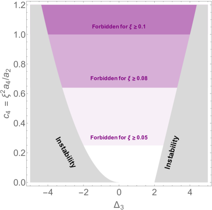
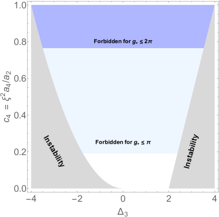
Figure 1: Parameter space for the cubic Higgs self-coupling deformation $\Delta_{3}$ relative to the SM value. The allowed region depends on the value $c_{4}=\xi a_{4}/a_{2}$, which encodes effects of dimension-8 SMEFT operators in the Higgs potential. The gray area is excluded by stability considerations, as the potential contains a deeper minimum that the EW vacuum at $\langle H^{\dagger}H\rangle=v^{2}/2$. Left: the purple areas are excluded for $a_{4}=1$ and $a_{2}=0.01$ under different hypotheses about the parameter $\xi=v^{2}/f^{2}$, which characterizes the size of the corrections to the single Higgs boson couplings to matter. Right: the blue areas are excluded for $a_{4}=1$ and $\xi=0.1$ under different hypotheses about the coupling strength $g_{*}$ of the BSM theory underlying the SM.

To make the bound more precise, it is quantitatively adequate to focus on the case

$$\tilde{P}=1+{1\over 2}\Delta_{3}\tilde{X}+c_{4}{\tilde{X}}^{2},$$ (12)

given that the $|c_{n>4}|$ are anyway expected to be suppressed. The resulting constraints are shown in Fig. 1. Outside the region $0<\Delta_{3}<4$ the bound coincides with the condition for absolute positivity of $\tilde{P}$: $\Delta_{3}^{2}<16c_{4}$. Using the definition of $c_{4}$ in Eq. (10) we obtain

$$|\Delta_{3}|\lesssim 4\sqrt{a_{4}}\sqrt{0.01\over a_{2}}\left(\xi\over 0.1\right).$$ (13)

On the other hand, for $0<\Delta_{3}<4$, the bound is weaker corresponding to cases where $\tilde{P}$ becomes negative in the unphysical region $\tilde{X}<-1$. In particular, for $0\leq\Delta_{3}\leq 2$, $c_{4}$ is even allowed to vanish. All in all, we conclude that a correction to the Higgs cubic coupling in the range $0\leq\Delta_{3}\leq 2$ can be obtained under the very conservative assumption $a_{4}>0$. Larger or smaller values of $\Delta_{3}$ are possible, subject to assumptions about the coefficient $a_{4}$ such that Eq. (13) is satisfied. In particular $|\Delta_{3}|>4$ can only be achieved for $a_{4}\mathrel{\hbox to0.0pt{\lower 4.0pt\hbox{\hskip 1.0pt$\sim$}\hss}\raise 1.0pt\hbox{$>$}}{\mathcal{O}}(1)$ which seems less plausible. The maximal value is reached for a maximally strongly coupled BSM theory completing the SMEFT at the scale $m_{*}$. For more moderate (and perhaps more realistic) couplings, the bound is correspondingly stronger; for example under the condition $|a_{4}|<1$ one has $-1.7\lesssim\Delta_{3}\lesssim 2.4$ for $g_{*}=\pi$. Furthermore, as illustrated in Fig. 1, the bound can be tightened if the single Higgs couplings to matter are better constrained by experiment, leading to a stronger bound on the parameter $\xi$. Notice however that the region $0\leq\Delta_{3}\leq 2$ can still be covered even for relatively weak couplings. For instance for $a_{3}=1$, $a_{2}=0.1$ and $\xi=0.1$ one can reach up to $\Delta_{3}=2$.

One way to read our results is that there exists space for a strongly coupled accidentally light Higgs with sizable ${\mathcal{O}}(1)$ deviations in its self-couplings but compatible with all single Higgs and EW precision measurements ($\xi\mathrel{\hbox to0.0pt{\lower 3.0pt\hbox{\hskip 0.0pt$\sim$}\hss}\raise 1.0pt\hbox{$<$}}0.1$) and with a fundamental scale $m_{*}\sim g_{*}v/\sqrt{\xi}\mathrel{\hbox to0.0pt{\lower 3.0pt\hbox{\hskip 0.0pt$\sim$}\hss}\raise 1.0pt\hbox{$<$}}5$ TeV out of reach of present LHC direct searches.

3 Non-analytic Higgs potential (HEFT)

In the previous section we have demonstrated that, in the SMEFT framework with the parametric separation between BSM and EW scales, theoretical arguments and experimental constraints lead to an upper bound on the magnitude of the cubic self-coupling of the Higgs boson: $|\Delta_{3}|\lesssim$ few. In particular we showed that, at the price of a tuning of $m_{h}^{2}$ and $v^{2}$, an ${\mathcal{O}}(1)$ deviation $\Delta_{3}$ can be obtained consistently with present data and for a new physics scale $m_{*}$ above the present LHC reach. Essential in the derivation was the analytic dependence of the lagrangian on the Higgs doublet field $H$, which follows from the assumption that the heavy states are massive regardless of EW symmetry breaking. In this section we discuss the cubic self-coupling in a setting where the analyticity assumption is removed. We shall see that, going beyond the SMEFT, there is an obstruction to achieving the separation between the BSM and EW scales. This other scenario is therefore subject to much more severe constraints coming from direct and indirect searches for new physics.

Consider, for concreteness, a simple scenario of an EFT where the Higgs boson self-interactions are described by the potential

$$V(h)={m_{h}^{2}\over 2v}\left(1+\Delta_{3}\right)h^{3}+{m_{h}^{2}\over 8v^{2}}h^{4}.$$ (14)

where the only deviation from the SM resides in the cubic coupling. In particular all $h^{n}$ terms with $n\geq 5$ are absent. Note that such a pattern cannot be obtained from any $SU(2)_{W}\times U(1)_{Y}$ invariant potential that is an analytic function of $H^{\dagger}H$. In particular, it cannot be obtained in the SMEFT, unless the entire infinite tower of higher-dimensional operators contributes to the potential. That situation however corresponds to $f\sim v$, which is phenomenologically very implausible. On the other hand, Eq. (14) belongs to the parameter space of the so-called HEFT, which is an effective theory where only the $U(1)_{Q}$ part of the EW symmetry is linearly realized. In the HEFT, the Goldstone bosons eaten by $W$ and $Z$ transform non-linearly under the full EW symmetry, while the Higgs boson $h$ is a perfect singlet. As a consequence, the general potential $V=v^{4}\sum_{n=2}^{\infty}c_{n}(h/v)^{n}$ with arbitrary coefficients $c_{n}$ is allowed by the symmetries, and Eq. (14) represents one particular direction within the HEFT parameter space.

It is illuminating to rewrite Eq. (14) in a manifestly $SU(2)_{W}\times U(1)_{Y}$ invariant language:

$$V(H)={m_{h}^{2}\over 8v^{2}}\left(2H^{\dagger}H-v^{2}\right)^{2}+\Delta_{3}{m_{h}^{2}\over 2v}\left(\sqrt{2H^{\dagger}H}-v\right)^{3},$$ (15)

where $H$ is the Higgs field in Eq. (1). In the unitary gauge, $\pi_{i}=0$, this potential reduces Eq. (14). We should mention that we are not aware of a concrete UV-complete model that would lead to exactly Eq. (15) in the low-energy effective theory. However, there do exist familiar examples where integrating out heavy degrees of freedoms yields non-analytic effective interactions. One is the SM plus a chiral 4th generation which, when integrated out at one loop, generates $V\supset(H^{\dagger}H)^{2}\log(H^{\dagger}H)$. Another is a model with the second Higgs doublet $\Phi$ and the potential $V_{\rm UV}=\kappa|\Phi|^{4}+\mu(\Phi^{\dagger}H+{\rm h.c.})$, where integrating $\Phi$ at tree level yields $V\supset(H^{\dagger}H)^{2/3}$. Yet another example is the model of Ref. [21], which in a certain parametric limits leads to an $h$ tadpole in the effective potential, thus $V\supset(H^{\dagger}H)^{1/2}$. It will be clear from the following discussion that the precise form of Eq. (15) is not important for our argument, as long as the potential is described by a non-analytic function of $H^{\dagger}H$.

For this discussion it is more convenient to work with the linear parametrization of the Higgs doublet: $H={1\over\sqrt{2}}\left(\begin{array}[]{c}iG_{1}+G_{2}\\ v+h+iG_{3}\end{array}\right)$. Then, outside the unitary gauge, the lagrangian in Eq. (15) contains interactions between the Higgs and the Goldstones:

$$V\supset\Delta_{3}{m_{h}^{2}\over 2v}\left(\sqrt{(h+v)^{2}+G^{2}}-v\right)^{3},$$ (16)

where $G^{2}\equiv G_{i}G_{i}$, and we do not display the Goldstone-Higgs interactions originating from the analytic SM part of the potential. By the equivalence theorem [22], these correspond to interactions of longitudinal components of the $W$ and $Z$ bosons at high energies. This way, the non-analytic terms effectively introduce hard contact interactions between $W_{L}/Z_{L}$ and an arbitrary number of Higgs bosons. In particular, expanding Eq. (15) in $G^{2}$, the terms with two Goldstone boson fields are

$$V \supset \Delta_{3}{3m_{h}^{2}\over 4v}{G^{2}h^{2}\over h+v}=\Delta_{3}{3m_{h}^{2}\over 4}G^{2}\sum_{n=2}^{\infty}\left(-h\over v\right)^{n}.$$ (17)

We can see that, for any non-zero $\Delta_{3}$, Eq. (17) contains higher-order interactions of the Higgs and Goldstone boson suppressed only by the EW scale $v$. It is thus clear that an EFT with the scalar potential in Eq. (14) must have a low cut-off scale, $m_{*}\lesssim 4\pi v$.

The need for a UV-completion below a certain scale manifests itself as a breakdown of perturbation theory around that scale. This always happens because of the presence of interaction terms of dimension $>4$ in the lagrangian, carrying coefficients with negative mass dimension. The critical operator dimension $4$ can be overcome by either powers of derivatives or powers of fields. In the more familiar case, like for instance 2-to-2 scattering of longitudinal vectors in the Higgsless SM [23], the loss of perturbativity is driven by derivative interactions which make amplitudes grow with energy. In the case at hand, like for massive fermions in the Higgsless SM  [24, 25], it is instead the presence of operators with an arbitrarily large number of legs that causes the breakdown of perturbation theory. Indeed, from Eq. (17), the tree-level 2-two-2 amplitude $GG\to hh$ is perfectly well-behaved and perturbative as long as $|\Delta_{3}|\lesssim{\mathcal{O}}(10)$. In order to quantify the validity regime of an EFT with the interactions in Eq. (17), we have to investigate $2\to n$ amplitudes with $n\geq 3$.

Before proceeding we would like to briefly review the logic of the standard estimates of the validity of the EFT. These are normally done by invoking the notion of breakdown of perturbative unitarity. This is conceptually fine as long as one does not interpret the issue of unitarity too strictly. Of course there is never an issue with unitarity, as the adjective perturbative implies. The point is simply and purely the breakdown of perturbation theory associated to the onset of a strong coupling regime. Focussing on the $S$-matrix, we know of course that unitarity is guaranteed, that is $S=e^{i\Delta}$ with $\Delta$ a Hermitian operator. The only issue concerns the ability to compute $\Delta$ in perturbation theory. $\Delta$ is a scattering phase operator, whose eigenvalues are defined modulo $2\pi$: the scattering phase shift is maximized when an eigenvalue equals $\pi$. The regime of weak coupling can thus be defined by the request $\delta_{i}\mathrel{\hbox to0.0pt{\lower 3.0pt\hbox{\hskip 0.0pt$\sim$}\hss}\raise 1.0pt\hbox{$<$}}\pi$ for the eigenvalues of $\Delta$. Now, the computation of the $S$ matrix in perturbation theory can be phrased as a computation of $\Delta$. In so doing unitarity is manifestly satisfied order by order in perturbation theory. Writing $S=1+iT$ we have $\Delta=-i\ln(1+iT)=T-iT^{2}+\dots$, so that in the Born approximation $\Delta$ and $T$ coincide: $\Delta_{0}=T_{0}$. A rough but reasonable way to require perturbativity is thus to ask for

$$\langle\Psi|T_{0}^{\dagger}T_{0}|\Psi\rangle\mathrel{\hbox to0.0pt{\lower 3.0pt\hbox{\hskip 0.0pt$\sim$}\hss}\raise 1.0pt\hbox{$<$}}\pi^{2}$$ (18)

for any incoming state $|\Psi\rangle$. Considering elastic 2-to-2 scattering one can easily check that this prescription produces the usual NDA bounds on couplings  [26, 27, 28]. In what follows we shall simply apply this to the processed $GG\to h^{n}$.

Consider a family of scattering amplitudes of the isospin-0 two-Goldstone state $|[GG]_{I=0}\rangle\equiv{\sum_{i}|G_{i}G_{i}\rangle\over\sqrt{3}}$. From Eq. (17), the leading high-energy contribution to the inelastic amplitude for scattering this state into $n$ Higgs bosons is given by

$${\mathcal{M}}([GG]_{I=0}\to\underbrace{h\dots h}_{n})\approx(-1)^{n+1}\Delta_{3}{3\sqrt{3}n!m_{h}^{2}\over 2v^{n}},$$ (19)

and the corresponding s-wave amplitude is ${\mathcal{M}}([GG]_{I=0}^{l=0}\to h^{n})={1\over 4\sqrt{\pi}}{\mathcal{M}}([GG]_{I=0}\to h^{n})$. A $2\to n$ amplitude with $n>2$ that is not suppressed at large energies leads to onset of strong coupling at some finite value $\Lambda_{*}$ of the center-of-mass energy $\sqrt{s}$. Indeed taking $|\Psi\rangle$ to coincide with the $s$-wave $GG$ state $|[GG]_{I=0}^{\ell=0}\rangle$ the bound in eq. (18) is easily seen to read

$$\left.\sum_{n=2}^{\infty}{1\over n!}\int d\Pi_{n}|{\mathcal{M}}([GG]_{I=0}^{l=0}\to h^{n})|^{2}\right|_{\sqrt{s}=\Lambda_{*}}=\sum_{n=2}^{\infty}{1\over n!}V_{n}(\Lambda_{*})|{\mathcal{M}}([GG]_{I=0}^{l=0}\to h^{n})|^{2}\sim\pi^{2},$$ (20)

where $V_{n}(x)=\int d\Pi_{n}={x^{2n-4}\over 2(n-1)!(n-2)!(4\pi)^{2n-3}}$ is the volume [29] of the n-body phase space in the limit the $m_{h}\to 0$. Inserting the explicit form of the amplitude and performing the sum over $n$, the above condition reduces to

$$\Delta_{3}^{2}{27m_{h}^{4}\over 512\pi^{2}v^{4}}\left(2+{\Lambda_{*}^{2}\over(4\pi v)^{2}}\right)\exp\left({\Lambda_{*}^{2}\over(4\pi v)^{2}}\right)\sim\pi^{2},$$ (21)

By definition $m_{*}\leq\Lambda_{*}$, from which we obtain the unitarity bound on the BSM scale:

$${m_{*}\over 4\pi v}\lesssim 2\log^{1/2}\left(4\pi v\over m_{h}|\Delta_{3}|^{1/2}\right)\sim{\mathcal{O}}(1).$$ (22)

For $|\Delta_{3}|\sim 1$ the maximum scale of the UV completion is parametrically of order $4\pi v\sim 3$ TeV, as expected. In fact, that scale is only logarithmically sensitive to the magnitude of $|\Delta_{3}|$, and thus remains of order $4\pi v$ even for $|\Delta_{3}|\ll 1$. In this bound we have only considered the $h^{n}$ final states. In reality, final states involving any number of $GG$ pairs are equally important. Our computation thus represents a lower bound of $\langle\Psi|T_{0}^{\dagger}T_{0}|\Psi\rangle$, while the true upper bound on the cut-off is lower. Further optimization of the bound is possible by exploiting $n\to n$ scattering of special multi-particle Higgs and Goldstone states [31]. These improvements do not change the parametric dependence of the limit in Eq. (22), and are not essential for our argument.

It is clear from our argument that the bound on $m_{*}$ will depend little on the precise form of Eq. (14). A similar bound can be derived whenever the potential (or any other part of the lagrangian) contains terms non-analytic in $H^{\dagger}H$ that cannot be removed by field redefinitions or equations of motion. In such a case, higher-dimensional interaction terms between Higgs and Goldstone bosons are suppressed only by powers of the EW scale $v$, leading to an onset of strong coupling in $2\to n$ amplitudes at the scale of order $4\pi v$. Such a set-up is equivalent to the SMEFT with the expansion parameter $m_{*}\lesssim 4\pi v$, where gauge invariant operators with large canonical dimensions may dominate contributions to scattering amplitudes. Only when the EFT lagrangian is analytic in $H^{\dagger}H$, and its terms organized as an expansion in $1/m_{*}$ with $m_{*}\gg m_{h}$, can the validity regime of the EFT be parametrically extended above the EW scale. Such an EFT is a low-energy approximation of BSM models with the scale separation $m_{*}\gg m_{h}$, which were discussed in Section 2.

4 Conclusions

In this paper we derived bounds on the Higgs boson self-interactions, which are valid when the mass scale $m_{*}$ of BSM particles is hierarchically larger than the EW scale. Under this assumption the low-energy EFT describing Higgs interactions at the EW scale is the SMEFT, organized as an expansion in $1/m_{*}$. Corrections to the cubic couplings arise at ${\mathcal{O}}(m_{*}^{-2})$, that is from dimension-6 operators in the SMEFT lagrangian. Power counting suggests that the relative correction $\Delta_{3}$ to the cubic Higgs coupling can be enhanced when the BSM theory at $m_{*}$ is strongly coupled, such that $\Delta_{3}\gtrsim{\mathcal{O}}(10)$ even if corrections to other Higgs couplings are ${\mathcal{O}}(10\%)$. However, this simple estimate ignores the issue of vacuum stability. Taking that carefully into account, we found the allowed and excluded parameter regions displayed in Fig. 1, which is the central result of this paper.

Enhancement of the cubic in the range $0\leq\Delta_{3}\leq 2$ is possible under very broad assumptions. In particular, corrections in this range are robustly compatible with $\xi\sim 0.1$ and with $m_{*}$ ranging from $\sim 1$ TeV for weak coupling to $\sim 5$ TeV for strong coupling. A significant portion of this region is therefore outside the present reach of LHC data. On the other hand, outside the range $0\leq\Delta_{3}\leq 2$, vacuum stability depends on the pattern of SMEFT operators with dimensions higher than six, which in turn depends on the details of the BSM theory at the scale $m_{*}$. In view of that, it is impossible to derive sharp bounds, however, given the present experimental constraints on $\xi$, values $|\Delta_{3}|\mathrel{\hbox to0.0pt{\lower 4.0pt\hbox{\hskip 1.0pt$\sim$}\hss}\raise 1.0pt\hbox{$>$}}4$ appear rather implausible, even allowing for a maximally strongly coupled BSM theory. Stronger limits on $\Delta_{3}$ hold for moderate $g_{*}$ or for smaller $\xi$, as visible in Fig. 1. The bottom line is that, in the case $|\Delta_{3}|\gg 1$ is measured by experiment, we immediately learn important facts about the microscopic theory underlying the SM. First of all, it has to be rather strongly coupled. Furthermore, the parameter $\xi$ should be at least a few percent, which implies that BSM deviations in single Higgs boson couplings may also be within the LHC reach. The flip side of that last statement is that improved limits on the single Higgs couplings will translate into a stronger bound on $\Delta_{3}$.

It is important to stress that the upper values of $\Delta_{3}$, indeed $\Delta_{3}={\mathcal{O}}(1)$, can never be obtained in the more natural models of EW symmetry breaking, like composite Higgs or supersymmetric models. In those models, even when the Higgs is strongly coupled, there is a symmetry controlling the size of all terms in the Higgs potential. Indeed in the case of generic composite Higgs models one has $\Delta_{3}\sim\xi$ like for all other Higgs couplings. Our scenario for maximizing $\Delta_{3}$ while keeping $m_{*}$ above the weak scale crucially relies on $m_{h}$ and $v$ being suppressed with respect to their natural values, $m_{*}$ and $f$. That is completely consistent, but necessarily accidental or fine tuned.

Obviously, our bounds are not set in stone. There is always the possibility of a theory with either $m_{*}\mathrel{\hbox to0.0pt{\lower 3.0pt\hbox{\hskip 0.0pt$\sim$}\hss}\raise 1.0pt\hbox{$<$}}1$ TeV or $\xi\sim 1$ escaping, via multiple tunings, all phenomenological constraints from Higgs and EW precision measurements and from direct searches. Still, given the outcome of direct BSM searches at the LHC, as well as a wide range of precision measurements that returned results consistent with the SM predictions, we believe that to be a less likely option to enhance $\Delta_{3}$ than our accidentally light Higgs. For this reason we believe that the bounds presented in this paper are robust.

We also investigated a more general EFT where the Higgs potential at the EW scale cannot be written as a power series in $H^{\dagger}H$. We studied corrections to the cubic Higgs self-coupling that, in a $SU(2)_{W}\times U(1)_{Y}$ invariant language, are described by a non-analytic function of $H^{\dagger}H$. At first sight, this scenario may offer more freedom to arrange for a large $\Delta_{3}$ without violating stability or experimental constraints. We have shown however that in such a setting there is an obstruction to decoupling $m_{*}$ from the EW scale, leading to $\xi\sim 1$. Namely, $2\to n$ amplitudes for scattering of longitudinally polarized $W$ and $Z$ bosons into $n\geq 3$ Higgs bosons become strong and violate perturbative unitarity around the scale $4\pi v\approx 3$ TeV. Therefore, in this scenario it is impossible to have a sizable $\Delta_{3}$ while robustly satisfying all the constraints from single Higgs processes, EW precision measurements and direct searches. Again, it is not completely excluded that multiple tunings and/or clever model building [21, 32] may allow one to circumvent these phenomenological constraints.

Our analysis exemplifies the physical difference between Higgs EFTs with analytic and non-analytic potential. In the standard nomenclature, these EFTs go under the names of the SMEFT and the HEFT, respectively. Previously, the distinction between the two theories was described in a less intuitive language of linearly or non-linearly realized symmetries. Both of these EFTs have the same particle spectrum (that of the SM), however the HEFT is usually introduced as a more general theory where the $SU(2)_{W}\times U(1)_{Y}$ symmetry acts in a non-linear way on the Goldstone bosons, while the Higgs boson $h$ is an EW singlet. This results in more freedom in writing the Higgs potential at the leading order in the EFT expansion. In this paper we provided a clear and intuitive dynamical distinction between the SMEFT and the HEFT. We argued that the HEFT can be equivalently formulated with a linearly realized $SU(2)_{W}\times U(1)_{Y}$ symmetry, provided one allows in the lagrangian terms that are non-analytic in $H$ around $H=0$. In our classification analyticity versus non analyticity in $H$, modulo field redefinitions, is what distinguishes SMEFT from HEFT. In this paper we discussed only the Higgs potential, but the same classification can be used to distinguish SMEFT vs HEFT at the level of Higgs interactions with other fields. Our classification is not just a matter of aesthetics and directly concerns the dynamics. Indeed the non-analyticity in $H$ makes manifest, via the equivalence theorem, the existence of the strong $2\to n$ amplitudes mentioned in the previous paragraph, which prohibit extending the validity of that HEFT above the scale $4\pi v$ . Therefore, the HEFT is an appropriate low-energy description for non-decoupling BSM models with the mass scale close to a TeV. Conversely, BSM models with the mass scale $m_{*}$ parametrically larger than the EW scale are described at low energies by the SMEFT.

References

- [1] ATLAS, CMS collaboration, G. Aad et al., Measurements of the Higgs boson production and decay rates and constraints on its couplings from a combined ATLAS and CMS analysis of the LHC pp collision data at and 8 TeV, JHEP 08 (2016) 045, [1606.02266].
- [2] ATLAS collaboration, G. Aad et al., Combination of searches for Higgs boson pairs in collisions at 13 TeV with the ATLAS detector, 1906.02025.
- [3] CMS collaboration, A. M. Sirunyan et al., Combination of searches for Higgs boson pair production in proton-proton collisions at 13 TeV, Phys. Rev. Lett. 122 (2019) 121803, [1811.09689].
- [4] M. McCullough, An Indirect Model-Dependent Probe of the Higgs Self-Coupling, Phys. Rev. D90 (2014) 015001, [1312.3322].
- [5] M. Gorbahn and U. Haisch, Indirect probes of the trilinear Higgs coupling: and , JHEP 10 (2016) 094, [1607.03773].
- [6] G. Degrassi, P. P. Giardino, F. Maltoni and D. Pagani, Probing the Higgs self coupling via single Higgs production at the LHC, JHEP 12 (2016) 080, [1607.04251].
- [7] S. Di Vita, C. Grojean, G. Panico, M. Riembau and T. Vantalon, A global view on the Higgs self-coupling, JHEP 09 (2017) 069, [1704.01953].
- [8] F. Maltoni, D. Pagani, A. Shivaji and X. Zhao, Trilinear Higgs coupling determination via single-Higgs differential measurements at the LHC, Eur. Phys. J. C77 (2017) 887, [1709.08649].
- [9] G. Degrassi, M. Fedele and P. P. Giardino, Constraints on the trilinear Higgs self coupling from precision observables, JHEP 04 (2017) 155, [1702.01737].
- [10] G. D. Kribs, A. Maier, H. Rzehak, M. Spannowsky and P. Waite, Electroweak oblique parameters as a probe of the trilinear Higgs boson self-interaction, Phys. Rev. D95 (2017) 093004, [1702.07678].
- [11] B. Henning, D. Lombardo, M. Riembau and F. Riva, Higgs Couplings without the Higgs, Phys. Rev. Lett. 123 (2019) 181801, [1812.09299].
- [12] W. Buchmuller and D. Wyler, Effective Lagrangian Analysis of New Interactions and Flavor Conservation, Nucl.Phys. B268 (1986) 621–653.
- [13] C. N. Leung, S. T. Love and S. Rao, Low-Energy Manifestations of a New Interaction Scale: Operator Analysis, Z. Phys. C31 (1986) 433.
- [14] LHC Higgs Cross Section Working Group collaboration, D. de Florian et al., Handbook of LHC Higgs Cross Sections: 4. Deciphering the Nature of the Higgs Sector, 1610.07922.
- [15] R. Contino, D. Greco, R. Mahbubani, R. Rattazzi and R. Torre, Precision Tests and Fine Tuning in Twin Higgs Models, Phys. Rev. D96 (2017) 095036, [1702.00797].
- [16] A. Glioti, R. Rattazzi and L. Vecchi, Electroweak Baryogenesis above the Electroweak Scale, JHEP 04 (2019) 027, [1811.11740].
- [17] L. Di Luzio, R. Grober and M. Spannowsky, Maxi-sizing the trilinear Higgs self-coupling: how large could it be?, Eur. Phys. J. C77 (2017) 788, [1704.02311].
- [18] G. Giudice, C. Grojean, A. Pomarol and R. Rattazzi, The Strongly-Interacting Light Higgs, JHEP 0706 (2007) 045, [hep-ph/0703164].
- [19] D. Liu, A. Pomarol, R. Rattazzi and F. Riva, Patterns of Strong Coupling for LHC Searches, JHEP 11 (2016) 141, [1603.03064].
- [20] R. Contino, A. Falkowski, F. Goertz, C. Grojean and F. Riva, On the Validity of the Effective Field Theory Approach to SM Precision Tests, JHEP 07 (2016) 144, [1604.06444].
- [21] J. Galloway, M. A. Luty, Y. Tsai and Y. Zhao, Induced Electroweak Symmetry Breaking and Supersymmetric Naturalness, Phys. Rev. D89 (2014) 075003, [1306.6354].
- [22] J. M. Cornwall, D. N. Levin and G. Tiktopoulos, Derivation of Gauge Invariance from High-Energy Unitarity Bounds on the s Matrix, Phys. Rev. D10 (1974) 1145.
- [23] B. W. Lee, C. Quigg and H. B. Thacker, Weak Interactions at Very High-Energies: The Role of the Higgs Boson Mass, Phys. Rev. D16 (1977) 1519.
- [24] F. Maltoni, J. M. Niczyporuk and S. Willenbrock, The Scale of fermion mass generation, Phys. Rev. D65 (2002) 033004, [hep-ph/0106281].
- [25] D. A. Dicus and H.-J. He, Scales of fermion mass generation and electroweak symmetry breaking, Phys. Rev. D71 (2005) 093009, [hep-ph/0409131].
- [26] A. Manohar and H. Georgi, Chiral Quarks and the Nonrelativistic Quark Model, Nucl. Phys. B234 (1984) 189–212.
- [27] A. G. Cohen, D. B. Kaplan and A. E. Nelson, Counting 4 pis in strongly coupled supersymmetry, Phys. Lett. B412 (1997) 301–308, [hep-ph/9706275].
- [28] M. A. Luty, Naive dimensional analysis and supersymmetry, Phys. Rev. D57 (1998) 1531–1538, [hep-ph/9706235].
- [29] R. Kleiss, W. J. Stirling and S. D. Ellis, A New Monte Carlo Treatment of Multiparticle Phase Space at High-energies, Comput. Phys. Commun. 40 (1986) 359.
- [30] V. V. Khoze, Perturbative growth of high-multiplicity W, Z and Higgs production processes at high energies, JHEP 03 (2015) 038, [1411.2925].
- [31] S. Chang and M. A. Luty, The Higgs Trilinear Coupling and the Scale of New Physics, 1902.05556.
- [32] S. Chang, J. Galloway, M. Luty, E. Salvioni and Y. Tsai, Phenomenology of Induced Electroweak Symmetry Breaking, JHEP 03 (2015) 017, [1411.6023].
- [33] R. Alonso, E. E. Jenkins and A. V. Manohar, Geometry of the Scalar Sector, JHEP 08 (2016) 101, [1605.03602].