Properties of meteors with double peaked light curves

Abstract

Twenty-one meteors showing double peaked light curves were analysed with observations collected with the Canadian Automated Meteor Observatory tracking system. Each event has orbital information, photometry, and at least one high-resolution observation. Two distinct light curve shapes were found: sudden double peaked curves, and smooth double peaked curves. The sudden peaked curves were produced by objects on asteroidal orbits and mostly showed noticeable fragmentation, while the smooth peaked curves were produced by cometary meteoroids and predominantly showed little to no visible fragmentation. An attempt to model these meteors as single bodies with two chemical components was unsuccessful, implying that fragmentation must be included in meteoroid ablation models.

1 Introduction

It is well known that meteoroids do not behave as the classical ablation model predicts, mainly because of fragmentation (Jacchia, 1955; Verniani, 1965; Weryk & Brown, 2012; Subasinghe et al., 2016). Observations are used as constraints in ablation models to improve our understanding of the processes occurring. The shape of a meteor light curve (the light produced as a function of time or height) is sometimes used to infer the grain size and distribution of fragments within the meteoroid (e.g. Beech & Murray, 2003; Campbell-Brown & Koschny, 2004; Borovička et al., 2007). The meteoroid origin, determined from its orbit, can suggest physical properties such as strength and porosity, and high-resolution optical observations independently confirm fragmentation processes. An analysis of these three types of observations (photometry, orbit, and high-resolution optical observations) was completed by Subasinghe et al. (2016) to investigate meteoroid behaviour. The results of that study found that meteoroids do not behave as expected: more than 90% of meteors observed in the high-resolution camera showed obvious fragmentation in some form; meteoroids that showed little to no visible fragmentation had mostly symmetric light curves rather than the expected classical late peaked light curve; and about a third (but likely fewer) of the meteor light curves showed unusual shapes. Asteroidal and cometary meteoroids were found to behave very similarly, in terms of light curve shape and fragmentation behaviour.

Despite the many constraints provided by these observations, it is still difficult to model meteoroid ablation. The classical meteoroid ablation model predicts the behaviour of a solid, single-bodied object that does not fragment: this is the simplest model and it does not work well (e.g. Jacchia, 1955; Koten et al., 2004) because most meteoroids fragment (Weryk et al., 2013; Subasinghe et al., 2016). Even when fragmentation is included in models and a good match is obtained for the light curve and deceleration, high-resolution observations from the Canadian Automated Meteor Observatory (CAMO) tracking system show the model limitations: Campbell-Brown et al. (2013) modelled ten meteors with two different fragmentation models and both predicted wakes which were both too long and too bright compared to the observed wakes. Campbell-Brown (2017) attempted to model an apparently single-body meteoroid which was one of the ten from Campbell-Brown et al. (2013), and found that a single-body ablation model was not able to reproduce the observations: the modelled light curve was too bright over too wide a range of heights compared to the observed curve. An ablation model in which the meteoroid fragments with many small bursts was more successful at reproducing both the light curve and the high resolution behaviour, indicating that it is possible to have fragmentation which does not produce a long visible wake.

The dustball model was proposed in 1975 by Hawkes & Jones who suggested that meteoroids are composed of two fundamental parts: grains with a high boiling temperature, and an organic glue with a lower boiling temperature, that holds the grains together. It has been suggested that the glue may be organic (Murray et al., 2000; Roberts et al., 2014), or may contain volatile sodium (Borovička et al., 2007), and in some cases is assumed not to contribute to the observed optical emission. The dustball model has been modified to include different fragmentation mechanisms and has been used successfully in recent years to reproduce meteor observations (Campbell-Brown & Koschny, 2004; Borovička et al., 2007).

Many studies have found that meteors show mainly symmetric light curves (e.g. Fleming et al., 1993; Koten et al., 2004; Subasinghe et al., 2016). Symmetric light curves can be explained by fragmentation with the dustball model. However, single-peaked light curves are not exclusively observed: some meteors have multi-peaked curves. The mechanisms behind double peaked curves are not well studied. Subasinghe et al. (2016) found that 18% of their analysed meteor light curves showed a double peaked shape, but suggest that the real contribution is lower due to false inflection points at the edges of the light curves due to the fitting method. Twenty-one double peaked meteor light curves were studied by Roberts et al. (2014), whose modelling work suggested that the light curves could be reproduced using a dustball model where some grains are released before intensive ablation begins, followed by a later release of larger grains. The range of grain masses used was 10^-12 to 10^-5 kg. Many of the events studied by Roberts et al. (2014) showed a rounded first peak, followed by a sharp increase in luminosity for the second peak. The model used in that work produced an almost instantaneous increase in brightness at the onset of the second peak. In this work, we look at meteors with double peaked light curves to study their physical properties.

2 Observations

2.1 Equipment

The observations for this work were collected with the Canadian Automated Meteor Observatory (CAMO) tracking system (Weryk et al., 2013). This is a two-station system, with a narrow-field and wide-field camera at each station. The two stations are located at Elginfield, Ontario, Canada (43.193^∘N, 81.316^∘W) and Tavistock, Ontario, Canada (43.265^∘N, 80.772^∘W) and are about 45 km apart. The wide-field cameras have a field of view of 26^∘ $\times$ 19^∘, and run at 80 frames per second. The narrow-field cameras have a field of view of 1.5^∘ $\times$ 1^∘, and run at 110 frames per second. In late October 2017 the Elginfield cameras were upgraded, and the field of view for the wide-field camera is now 34^∘ $\times$ 34^∘, and the narrow-field is 2^∘ $\times$ 2^∘.

From the wide-field observations the meteor light curve can be obtained, as well as the meteoroid trajectory (and orbit). The narrow-field cameras have resolutions as high as 3 metres per pixel at a range of 100 km, and are capable of capturing the fragmentation behaviour of the meteoroid.

2.2 Data

We used both wide and narrow-field observations from the CAMO system. The All Sky and Guided Automatic Realtime Detection (ASGARD) software detects meteors in the wide-field camera in real time, and directs a pair of mirrors to guide the meteor light into the narrow-field camera. ASGARD also provides a solution (trajectory and photometry) for each recorded wide-field meteor event. This is done by comparing pixels frame by frame, searching for clusters where the intensity exceeds five standard deviations above the mean background. If in at least three consecutive frames, a minimum of six pixels in an 8 $\times$ 8 pixel region have intensities greater than the predefined threshold, a meteor has been detected. ASGARD uses centroiding to select the head of the meteor in each frame and these position picks are used in MILIG, a least squares method trajectory solver (Borovicka, 1990). ASGARD also masks out meteor pixels with intensities greater than the background to determine the meteor photometry. The meteor photometry and astrometry are calibrated using manually made photometric and astrometric plates, in which a user selects typically more than 20 stars in the field of view, which are calibrated against those from the Sky2000v4 catalogue (Myers et al., 2001). More than 7000 ASGARD reductions were searched for meteors with double peaked light curves. Our initial search fit a curve to the observed wide-field photometry data, and selected those with three turning points.

After this search, the light curves of the potential candidates (1257 out of 7160 events) were manually checked to remove events whose automatic reductions were either erroneously flagged as double peaked due to noise or false inflection points at the start or end of the curve due to the fitting method, or events whose double peak was somewhat ambiguous. The remaining potential events (53 total) were then reduced using the software program METAL (METeor AnaLysis) (Weryk & Brown, 2012). METAL works in a similar way to ASGARD, but needs a human operator, which avoids the errors sometimes made by ASGARD in accidentally selecting a hot pixel, or nearby star. Any event that showed a double peak in its manually reduced wide-field photometry data (rather than oscillations in the light curve due to noise in the system, clouds, or poor photometric calibrations) had its narrow-field observation further reduced in the software program mirfit (33 events total). Two events are shown in Fig. 1: one shows an ASGARD reduction initially classified as multi-peaked, but was then rejected on the grounds that the two stations did not agree (the oscillations were due to noise); and a second event that was classified as double peaked based on the automated light curve, but proved to be single peaked when reduced manually.

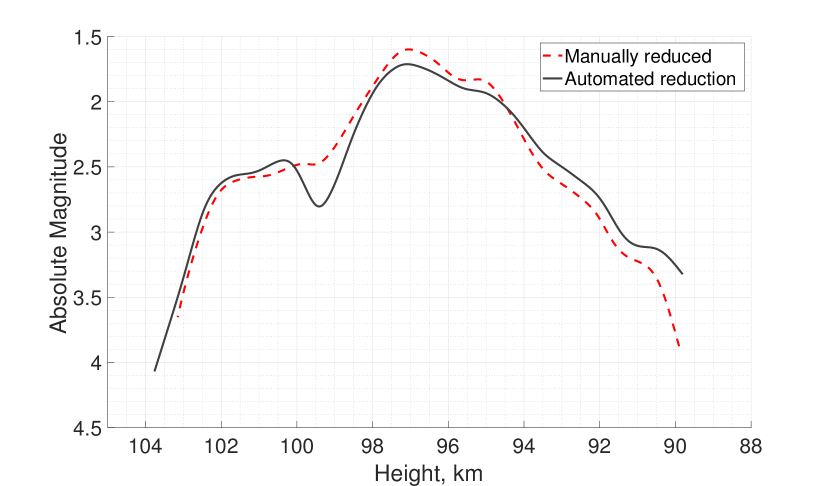
Figure 1: Examples of mis-categorized meteor light curves based on automatic ASGARD reductions. The top figure shows the Tavistock and Elginfield interpolated curves based on the observed data points, in red and blue. The two station observations disagree by up to half a magnitude. The gray curve is the interpolated curve based on both observations, and shows 9 turning points. Many of those turning points are within 0.5 magnitude and are likely due to noise in the system. The bottom figure shows two curves: the solid gray line shows the interpolated curve based on both station observations determined by ASGARD, and the red curve shows the manually reduced interpolated curve, showing that the trough was due to poor ASGARD photometry.

The software program mirfit allows observations collected with the high-resolution narrow-field cameras to be reduced. Meteors are manually reduced in mirfit in a similar way to METAL: the position of the head of the meteor is selected and the light from the meteor is masked out. Both the position of the meteor in the field and the position of the mirrors at the time of exposure are used in determining the angular position of the meteor in the sky. The meteor trajectory is determined using MILIG, and the log of the sum of the pixel brightness is determined. The absolute brightness of the meteor cannot be determined in mirfit due to the small field of view: there are typically not enough visible stars to compute a photometric calibration. The mirfit brightness values can be calibrated against the manually obtained absolute magnitude METAL light curve to determine the absolute magnitude mirfit light curve. In this work, we were not concerned with the mirfit photometry, so much as we were with the meteoroid fragmentation behaviour: did the meteoroid break into many small pieces, or a few large pieces? This can provide insight into the strength of the object and the processes it undergoes. The combined METAL and mirfit photometry for each event was manually assessed to determine whether to include the event in the final analysis (visually, how strong is the double peak? Is there good overlap between the wide and narrow-field observations? How well tracked was the event in the narrow-field camera?). This reduced our set of 33 events to 21.

These twenty-one double peaked events with their relevant parameters are listed in Table 1. Not all meteor events had two station narrow-field observations, meaning some fragmentation behaviour analysis was completed on single-station data only.

Table 1: Parameters of the double peaked meteor events. The given Tisserand parameter is determined with respect to Jupiter, the peak magnitudes and related heights are based on curves interpolated to the observations, and $z$ represents the zenith angle

. Event v_i $\alpha_{g}$ $\delta_{g}$ T_J Peak magnitudes Heights at peak magnitudes $a$ $e$ $i$ $z$ km s^-1 (^∘) (^∘) km AU (^∘) (^∘) 20100920_084608 60.30 50.10 19.01 0.8 1.1, 1.0 97.9, 92.7 3.7 0.94 178.00 24.9 20101009_060641 17.82 17.30 7.86 5.1 3.4, 4.7 81.8, 77.8 1.2 0.48 0.23 32.7 20110830_071519 59.88 27.44 43.59 0.4 1.7, 1.7 103.7, 99.0 5.8 0.88 119.86 15.9 20111005_084734 66.36 125.55 35.06 0.4 1.0, 0.8 101.5, 96.5 4.0 0.81 150.40 47.0 20111104_082320 69.77 131.65 36.16 -0.6 1.0, 0.6 190.8, 96.4 13.9 0.93 149.37 34.5 20120912_063437 38.01 14.54 20.28 4.1 3.2, 2.0 94.6, 90.9 1.4 0.92 36.34 23.5 20130816_081853 35.79 347.53 -8.28 3.1 3.6, 2.1 93.0, 89.9 2.0 0.91 5.50 53.8 20131114_095829 57.55 151.20 53.30 1.5 1.0, 2.4 105.6, 96.9 2.8 0.66 110.95 21.4 20140421_051749 40.74 244.33 20.64 1.5 1.8, 0.6 92.4, 88.9 5.3 0.89 57.27 38.4 20140904_070414 31.94 8.17 -10.65 4.1 2.1, 0.8 93.1, 90.1 1.5 0.83 19.80 52.9 20141102_102214 55.69 146.98 51.69 2.9 2.4, 2.1 100.1, 95.0 1.6 0.36 113.91 22.3 20150121_053147 23.20 115.56 15.41 3.0 0.8, 1.1 83.4, 79.6 2.5 0.74 3.68 27.0 20150121_084050 38.37 147.88 39.77 1.0 2.8, 4.4 88.0, 81.1 12.7 0.97 35.96 15.4 20150522_071644 62.73 314.90 16.24 0.3 2.3, 1.5 101.4, 96.2 5.7 0.83 124.58 48.5 20150925_083237 69.10 99.38 37.03 -0.1 1.5, 1.8 101.8, 97.0 5.2 0.81 155.67 37.3 20151210_082756 66.59 151.30 28.54 -0.5 0.9, 2.4 106.2, 98.7 16.6 0.96 146.83 26.6 20160808_083545 60.41 42.69 57.70 -0.4 2.8, -0.6 97.6, 91.6 167 0.99 112.23 27.4 20170824_023951 24.68 329.09 -3.97 3.1 2.0, 2.2 84.9, 80.0 2.4 0.75 5.85 55.8 20170924_070328 35.63 1.20 24.30 0.9 2.6, 4.5 92.7, 83.1 31.9 0.99 27.48 28.0 20171016_093056 40.87 47.22 20.57 2.6 3.0, 4.7 91.8, 80.9 2.3 0.97 9.44 38.8 20171201_103027 66.98 149.74 18.00 1.2 0.6, 0.8 101.4, 96.6 2.4 0.67 169.69 26.4

3 Results and Analysis

3.1 Light Curves

Two different categories of multi-peaked light curves became obvious during analysis: smooth double peaked, and sudden double peaked curves. Smooth peaked curves typically showed a shape similar to that shown in Fig. 2, increasing gradually in brightness in both peaks, while sudden peaked curves showed a much steeper, more instantaneous increase in brightness for the second peak, as shown in Fig. 3.

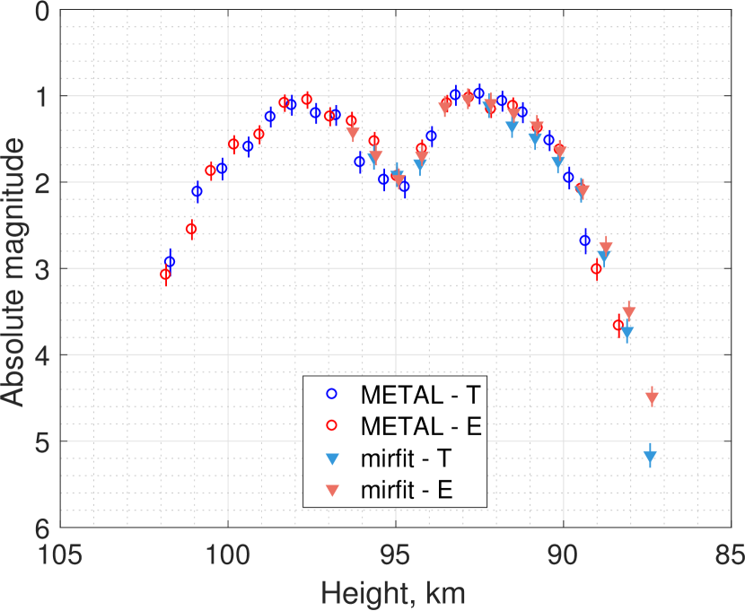
Figure 2: A typical ‘double peaked’ curve. This event was recorded on September 20, 2010 at 08:46:08 UTC.

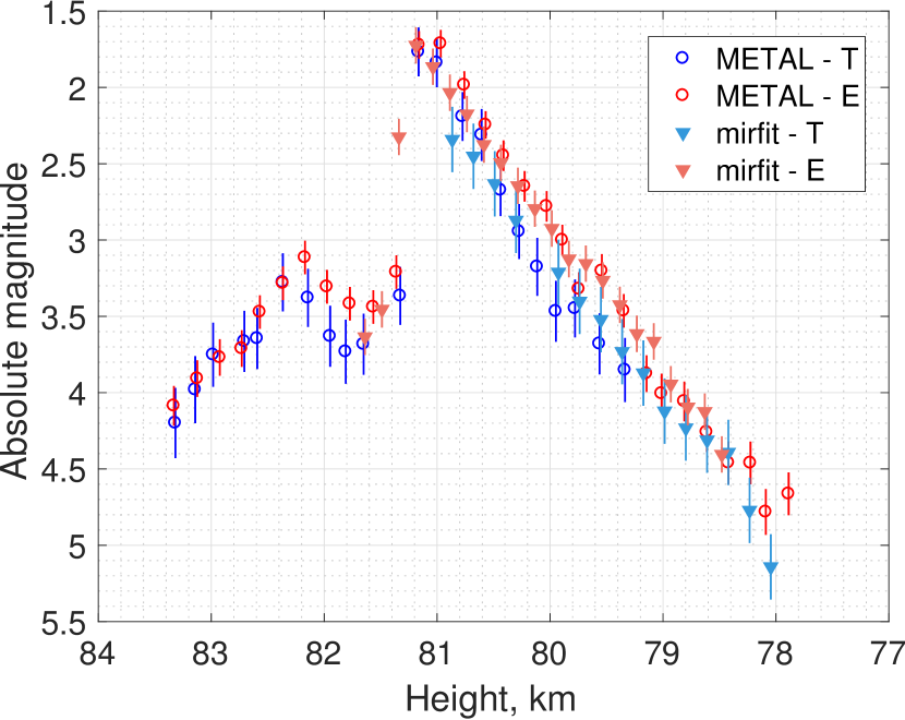
Figure 3: A typical ‘sudden peaked’ curve, recorded on October 9, 2010 at 06:06:41 UTC.

The steepness of the second peak was used to classify the light curves as either smooth double peaked, or sudden double peaked. Any event with a second peak rising slope greater than 1 mag/km was sorted into the sudden peaked group. The sudden peaked meteor events are listed in Table 2, along with a brief description of the fragmentation behaviour observed in the high-resolution narrow-field cameras. The smooth double peaked events are listed in Table 3.

3.2 Narrow-field observations

The fragmentation behaviour of each meteor was studied with the high-resolution narrow-field observations. Two station narrow-field observations were not available for all meteors, either due to poor weather or tracking issues at one of the stations. At a single station, the meteor events had at least 8 and sometimes more than 50 frames of narrow-field observations. A visual analysis of the observations was performed, and a description of the fragmentation behaviour is listed in Tables  2 and 3.

The meteor events were visually classified into one of five fragmentation types: long visible wake; short faint wake; line of motion fragmentation; elongated head with faint wake; or faint wake (single body). The categories used here are similar but not identical to those used in Subasinghe et al. (2016): our groups here are more restrictive. Our categories of short faint wake and faint wake (single body) are similar to the Subasinghe et al. (2016) category of ‘round head/little to no wake/no distinct fragments’. Our categories of elongated head with faint wake and long visible wake are similar to the Subasinghe et al. (2016) category of ‘smeared head/distinct wake/no fragmentation’, but without the distinct wake for the events with elongated heads. Events in our line of motion fragmentation group would fall under the ‘one of more noticeable fragments’ group. Examples of each category are shown in Fig. 4.

Table 2: Sudden peaked meteor events. Column H_x describes the amount of light produced by the head at station 1 or 2, and T_x describes the amount of light produced by the wake, at one of the two stations. Column ht_avg,x lists the average height at which the light produced values were calculated. The narrow-field description and the amount of light produced values do not necessarily correspond, since the light produced values are averaged over a number of frames, and the meteor appearance changes greatly during ablation. These sudden peaked events had a second peak rising slope greater than 1 mag/km, with their second peak slope value given in column $m_{2}$.

Event	vi	TJ	Narrow-field description	H1	T1	htavg,1	H2	T2	htavg,2	$m_{2}$
	km s-1			%	%	km	%	% km		mag km-1
20101009_060641	17.82	5.1	long visible wake	52	48	79	57	43	80	3.2
20120912_063437	38.01	4.1	faint wake (single body)				67	33	88	1.2
20130816_081853	35.79	3.1	line of motion fragmentation	34	66	86				1.6
20140904_070414	31.94	4.1	line of motion fragmentation	52	48	91				1.2
20170824_023951	24.68	3.1	line of motion fragmentation	49	51	80	50	50	80	3.7

Table 3: Smooth double peaked meteor events. Column H_x describes the amount of light produced by the head at station 1 or 2, and T_x describes the amount of light produced by the wake, at one of the two stations. Column ht_avg,x lists the average height at which the light produced values were calculated. The amount of light produced by the head and wake of the meteor may not agree with the narrow-field description, as these are values that are averaged over many frames, during which the meteor appearance changed. These smooth double peaked events had a second peak rising slope less than 1 mag/km, with their second peak slope value given in column $m_{2}$.

Event	vi	TJ	Narrow-field description	H1	T1	htavg,1	H2	T2	htavg,2	$m_{2}$
	km s-1			%	%	km	%	%	km	mag km-1
20100920_084608	60.30	0.8	long visible wake	79	21	91	72	28	92	0.5
20110830_071519	59.88	0.4	short faint wake	77	23	98	75	25	99	0.2
20111005_084734	66.36	0.4	elongated head with faint wake				81	19	97	0.8
20111104_082320	69.77	-0.6	faint wake (single body)	80	20	100	67	33	105	0.5
20131114_095829	57.55	1.5	faint wake (single body)	86	14	98				0.5
20140421_051749	40.74	1.5	long visible wake	56	44	98				0.9
20141102_102214	55.69	2.9	faint wake (single body)	77	23	93	73	27	91	0.6
20150121_053147	23.20	3.0	long visible wake				64	36	82	0.5
20150121_084050	38.37	1.0	faint wake (single body)				70	30	87	0.6
20150522_071644	62.73	0.3	short faint wake	100	0	91	48	52	99	0.6
20150925_083237	69.10	-0.1	faint wake (single body)	70	30	93	66	34	97	0.3
20151210_082756	66.59	-0.5	long visible wake				87	13	102	0.3
20160808_083545	60.41	-0.4	elongated head with faint wake				82	18	100	0.8
20170924_070328	35.63	0.9	line of motion fragmentation	56	44	90	66	34	90	0.2
20171016_093056	40.87	2.6	long visible wake				79	21	87	0.4
20171201_103027	66.98	1.2	short faint wake	90	10	93	82	18	93	0.3

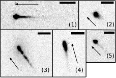
Figure 4: The five morphologies that were observed in the meteor events. Each example is from a different event, showing a single frame of the narrow-field observation, with the colour inverted to show detail. (1) shows a meteor with a long visible wake; (2) shows a meteor with a short faint wake; (3) shows a meteor with fragmentation along the line of motion; (4) shows a meteor with an elongated head and faint wake; and (5) shows a meteor that has faint wake and looks almost single bodied. The scale bar in each frame is 100 m, and the arrow indicates the direction of motion.

3.3 Trail brightness profiles

In order to quantify the different fragmentation behaviour of the meteors, the fraction of light produced at the head of the meteor compared to the wake was analysed. The software program mirfit extracts for each selected meteor position in a frame, the sum of pixel brightness values for each transverse slice of the meteor as a function of distance along the trail. This gives a brightness profile for each frame, and can be used to study the contribution of light originating at the head of the meteor versus the wake. The brightness profile from a single frame is shown in Fig. 5. To determine the amount of light coming from the head of the meteor, the size of each meteor head was determined in the image analysis program ImageJ (Schneider et al., 2012). Each head was assumed to be circular, and an average radius in pixels was manually determined. To determine the size of the head of the meteor in a given frame, a circle was fit to the meteor with the diameter equal to that of a transverse slice through the widest part of the meteoroid. Variations in brightness as well as smearing in the tracking system caused the size of meteor head to be different from meteor to meteor, and even from frame to frame of the same meteor event. An example of the variation in meteor appearance is given in Fig. 6. For each frame, the fraction of light originating from the head of the meteor was determined, and the mean value from all the frames at a station was calculated. Values for the light coming from the meteoroid head and wake are given as percentages in Tables 2 and 3. These are mean values determined based on all frames at a given station which had meteor position picks in the narrow-field cameras. Tables 2 and 3 also give the mean height for these mean calculated brightness values. Fig. 7 shows examples of the observed wide-field light curve data, over-plotted with the narrow-field observations, where the colour of the narrow-field observation describes the fraction of light originating from the head of the meteoroid. These brightness profile-light curves can be found for all meteor events in the Appendix.

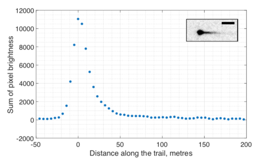
Figure 5: The brightness profile for meteor event 20100920_084608, Tavistock, frame 96. Each sum of pixel brightness value corresponds to a transverse slice through the meteor. The brightness profile is inset with the corresponding frame taken from the narrow-field observation. The scale bar is 100 m, and the colours have been inverted.

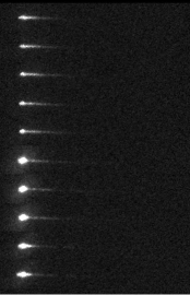
Figure 6: Frames from meteor 20171016_093056, which have been cropped, rotated and stacked to show the evolution. Time increases downwards. A circle was fit to the head of the meteor, with reference to the brightness profile. It is clear that the radius of that circle would increase, in this example, as ablation progresses. For simplicity, the mean radius from all frames with a meteor position pick was used to determine the size of the meteor head.

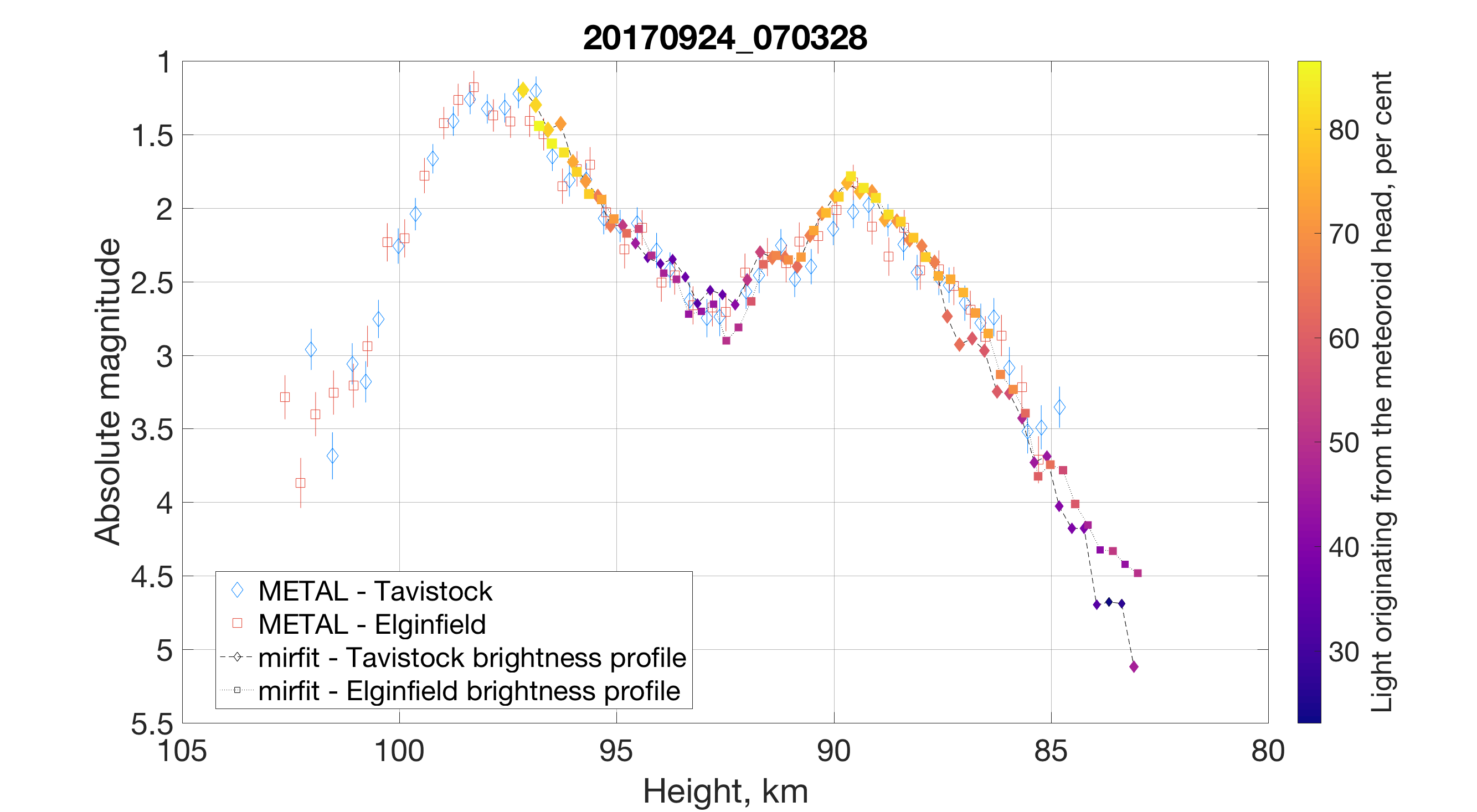
Figure 7: Two meteor events with their narrow-field observations plotted such that the size and colour of the symbol indicates the percentage of light originating from the meteoroid head. The top figure shows what the majority of the brightness profile observations look like: the greatest amount of light coming from the meteoroid head occurs near the peaks, and the amount decreases with fainter magnitudes. The bottom figure shows a brightness profile only seen on one event: the greatest amount of light coming from the head occurred before the first peak, and the first peak shows more equal amounts of light coming from the head and wake. The second peak shows the greatest amount of light from the head occurring at the peak.

3.4 Modelling

The cause of the two peaks is not clear, as the above observations show a variety of behaviour from these meteoroids in origin, speed, and fragmentation. About half of these observed events show very faint wakes, which implies that bursts of fragmentation, as suggested by Roberts et al. (2014), are not a main contributor. Here, we attempted to model double peaked meteors without fragmentation, using a two-component single body ablation code. This model is described in detail in Campbell-Brown (2017), and a summary is given here. This inhomogeneous implementation of the single-body meteoroid model allows a meteoroid to have components with two or more chemical compositions and properties. Each component has its own mass, density, heat of ablation, boiling and melting temperatures, specific heat, condensation coefficient, molar mass, thermal conductivity, and luminous efficiency. The components are assumed to be well mixed, so that each can ablate independently. The meteoroid heats uniformly, and is able to have a non-zero porosity, which can change if one component ablates faster than the other, and can drop to zero at a specified temperature, to simulate the meteoroid fully melting and becoming a non-porous droplet. This model is able to produce non-classical light curves, without fragmentation. This is important for this work as many of the meteors studied here show little to no visible wake (eleven of our twenty-one events were classified as having faint wake or appearing single-body like).

We considered a two component meteoroid, in which each component could have one of three possible masses (which affects the total mass of the meteoroid, and the ratio of the masses of the two components); one of five possible densities; and one of five heats of ablation. All other parameters were kept constant and identical between the two components due to their weaker influence on the resulting meteor light curve. The values that were varied (mass, density, heat of ablation) are given in Table 4, and the other parameter values are given in Table 5. The initial speed of each meteoroid was set to 30 km s^-1. Each combination of parameters was used to simulate a meteor, resulting in 5625 simulations. The results are discussed in 4.2

Table 4: The parameters that were varied in the simulations, and their possible values.

Mass	Density	Heat of Ablation
kg	kg m-3	106 J kg-1
10-4	500	0.5
10-5	1000	1
10-6	2000	2
	3000	4
	8000	6

Table 5: The simulation parameters that were not varied. Both meteoroid components had the following identical parameters for every simulation.

Porosity	Boiling	Melting	Specific	Condensation	Molar	Thermal	Luminous	Shape	Emissivity	Zenith
	Point	Point	heat	Coefficient	Mass	Conductivity	Efficiency	Factor		Angle
	K	K	J kg-1K	psi	atomic units	J m-1s-1K-1	per cent			degrees
0	2100	2000	1000	0.5	40	3	0.7	1.21	0.9	45

4 Discussion

The observed meteor light curves show two distinct shapes: a smooth double peaked curve, which reaches a maximum, decreases in brightness, and then smoothly repeats the process, and a sudden double peaked light curve, which typically shows a smooth increase in magnitude, followed by a slight decrease and a sharp linear increase in brightness. This sudden change is on average an increase of 2.2 mag per 1.0 km height decrease. The first peak for two of the sudden peaked events is not clear due to noise and the faintness of the event (see 19 and 20 in the Appendix).

The origin of a small Solar System body can be inferred using its Tisserand parameter. A Tisserand parameter greater than three is suggestive of an asteroidal origin; values between two and three are associated with Jupiter family comets; and values less than two are often related to long period comets. The boundaries between these groups are not concrete: objects may show asteroidal properties but have cometary Tisserand values. Despite this, the Tisserand parameter provides a method for associating a meteoroid with a broad class of parent body.

We find that the sudden peaked meteor events have Tisserand values greater than 3, associating them with asteroidal orbits. The smooth peaked meteor events have Tisserand parameter values less than 3 (except for one event, with a Tisserand of 3.0), associating them with cometary bodies.

We also considered the K_b parameter of each double peaked meteor. The K_b parameter, defined by Ceplecha (1958) is used to classify meteors based on their strength, and can be used to assign a density to a meteoroid. It assumes that all meteoroids begin their luminous phase at the same surface temperature. This implies that the meteor begin height is strongly related to the meteoroid composition. A K_b value less than 6.6 is associated with weak cometary material; values between 6.6 and 7.1 are associated with regular cometary objects; dense cometary objects have values between 7.1 and 7.3; carboneous chondrites are associated with values between 7.3 and 8; and values greater than or equal to 8 describe chondritic asteroidal material. To investigate our double peaked meteors and their K_b parameters, we plotted the begin height and initial speed of a large set (7160 events) of meteors which were automatically reduced by ASGARD. These meteors were coloured according to their Tisserand parameter (cometary or asteroidal). We then overplotted our double peaked meteor events, with shapes that describe their origin based on their Tisserand parameter (cometary or asteroidal) and with colours that describe their K_b parameter. This is shown in Figure 8. All the double peaked meteors from this study fall within the larger set of meteors, and roughly follow the split of cometary meteoroids having higher begin heights and speeds, and asteroidal meteoroids having lower begin heights and speeds, with no unusual values. In terms of K_b parameter, we have no double peaked events with values associated with the two extreme categories (weak cometary material, and chondritic asteroidal material).

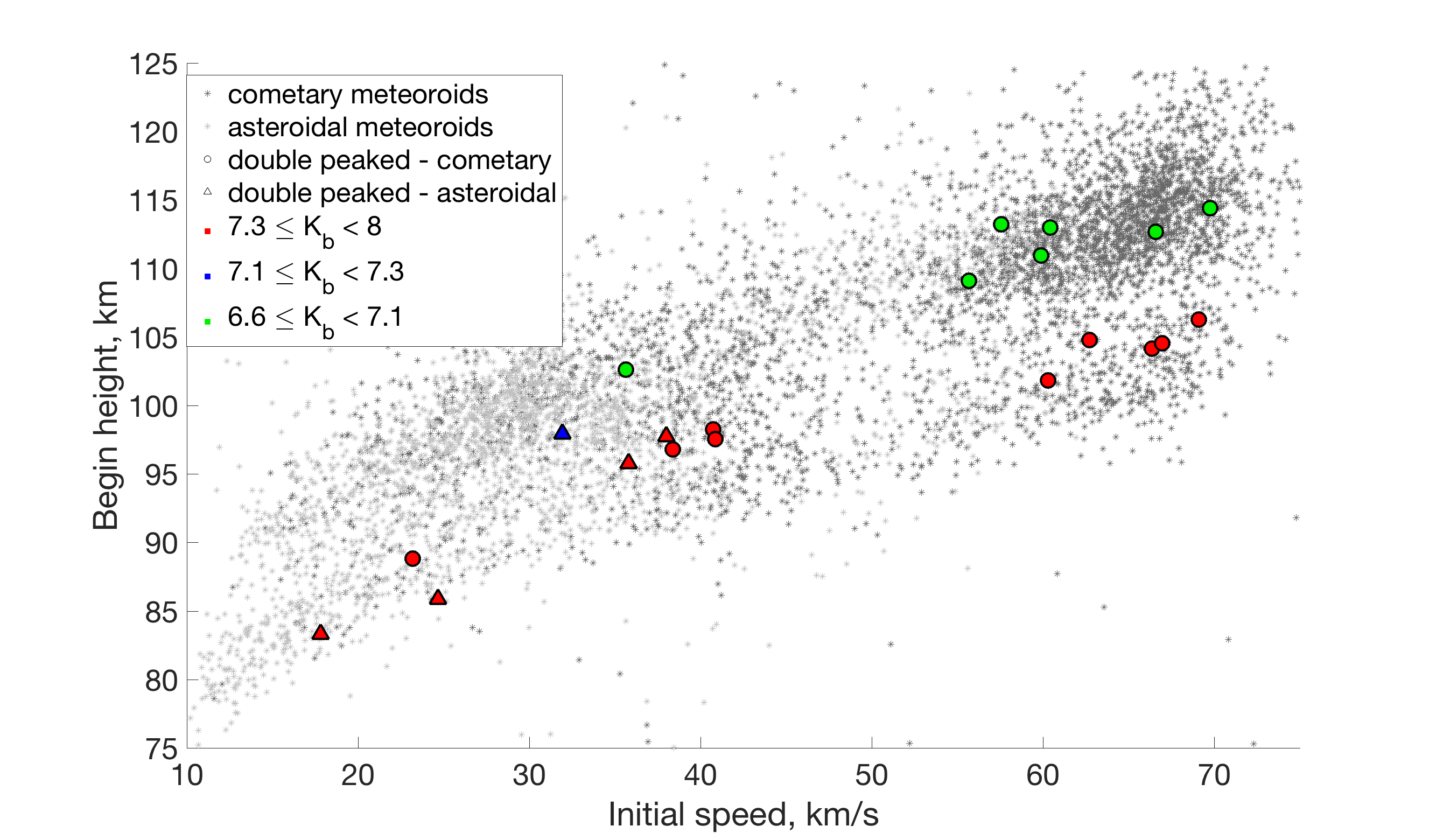
Figure 8: ASGARD reduced meteors are shown as asterisks: dark gray for cometary meteoroids, and light gray for asteroidal meteoroids based on their Tisserand values. The double peaked events in this study are plotted as circles if they are cometary in origin, or triangles for those that are asteroidal. The double peaked meteors are then coloured by their K_b values. For interpretation of the references to colour in this figure, the reader is referred to the web version of this paper.

The morphology of each meteor was analysed and manually categorized based on the extent of the visible wake; the shape of the meteor head; and whether gross fragmentation was occurring. The meteors were assigned to one of five categories, and examples are shown in Fig. 4. Many of the meteors in the smooth double peaked category (63%) show faint wakes or single body like behaviour, whereas only one fifth of the sudden peaked events show similar behaviour. The majority of the sudden peaked events show fragmentation, mainly in the form of gross fragmentation along the line of motion.

Asteroidal meteoroids are often assumed to be stronger than cometary meteoroids due to their origin. However, Subasinghe et al. (2016) found that asteroidal meteoroids fragment as often as cometary meteoroids (i.e. they found that asteroidal meteoroids showed a distinct trail or wake 87.2% of the time, compared to 86.8% for cometary meteoroids). We find similar results here: our sudden peaked meteors are all asteroidal in origin and 80% of the events show significant fragmentation. The smooth double peaked curves are all cometary in origin and about 70% of those events show fragmentation (five of the sixteen events were classified as looking single body like, and those events showed less wake than the other eleven events). We do note that this study has considerably fewer events to analyse.

The contribution of light for the sudden peaked events comes almost equally from the head and wake of the meteor for 3 of the 5 events. This is expected for a fragmenting object. For an object that is more single bodied and not fragmenting, the majority of the light is expected to be produced in the head of the meteor. However, the size of the meteor head changes over time, and because we used a mean size for the head, light from the meteor head may be incorrectly attributed to the wake, or vice versa. The smooth double peaked meteor events show mostly higher light contribution from the meteor head compared to the wake. The values from the two stations agree quite well with each other, and when they don’t (see 20150522_071644 for example), the disagreement is due to the height at which the observations were recorded (that is, the two stations observed different parts of the ablation profile). Appendix A shows each wide-field meteor light curve, with the narrow-field observations plotted as symbols in which the colour and size correspond to the percentage of light originating from the meteoroid head. Two of these events are reproduced in Fig. 7. For many events (18 of the 21), the brightness profiles clearly show that the amount of light coming from the head of the meteoroid is greatest at the peaks and minimal in the trough and decreases away from the peaks. One of the remaining three events has too few data points to make a conclusion (20140421_051749) and one event (20100920_084608) shows disagreement between the two stations at the end of the observation, where the absolute magnitude is fainter than +4. The remaining event (20150121_053137) shows that the greatest amount of light coming from the head occurred before the first peak, and decreased as the first maximum meteor brightness was observed. The meteoroid may be breaking up prior to the first peak, and the amount of light coming from the head, which was initially high, is now (at the first peak) coming more equally from the head and wake.

4.1 Possible mechanisms

Roberts et al. (2014) studied a set of double peaked meteor light curves observed with the CAMO tracking system. Some of the light curves of those meteors were successfully modelled using a dustball model. More details were obtained from the unpublished thesis (Roberts, 2014). In Roberts et al. (2014), both peaks were successfully modelled for nine events, and the second peak was successfully modelled for one event. Their implementation of the dustball model has a release of grains before the light curve is observed. As these grains ablate, the meteor increases in brightness, creating the first peak. When the meteor reaches a certain height (determined manually, and corresponding to the end of the first peak), another group of grains is released all at once. The luminosity of these grains produces the second peak. The first group of released grains were referred to as outer grains, and the second group as core grains; and they found that the core grains were more massive than the outer grains. There is no analysis of corresponding narrow-field observations for the group of 21 meteors studied in Roberts et al. (2014).

We find that a simultaneous release of many grains is not adequate to explain the second peak, as many of our events appear to be single body like (or show very faint wake). The Roberts et al. (2014) dustball model predicts an instantaneous linear increase in magnitude for the second peak. This model may be able to reproduce our sudden peaked light curves, which show mainly (80% of events) noticeable fragmentation. This model is unlikely to work on our other events which show minimal fragmentation at CAMO’s resolution, though they may be undergoing some form of continuous fragmentation, similar to that modelled in Campbell-Brown (2017). If a meteoroid were to fragment into identical grains, no wake would be expected, but this is an unlikely scenario.

Another potential mechanism for producing a multi-peaked light curve is differential ablation. In this process, more volatile species (sodium, magnesium, etc) ablate first, producing the first peak, followed by the more refractory species (e.g. calcium) which may produce the second peak. Differential ablation has been detected in meteor observations (Borovicka et al., 1999; Bloxam & Campbell-Brown, 2017). The work done by Bloxam & Campbell-Brown (2017) using a four camera spectral system, with CAMO, found that 94% of meteors showing differential ablation showed fragmentation in the corresponding narrow-field observation. Two of our double peaked meteor events fall into the collection period of the Bloxam & Campbell-Brown (2017) work, however no spectral data was observed for those events: the September 9 2015 event recorded very few frames (< 7) with the magnesium and sodium filters, which were affected by clouds; the December 10 2015 event was outside the field of view of all of the spectral cameras.

The physical structure of a meteoroid may also contribute to the object showing a multi-peaked light curve. This would be a type of differential ablation where the meteoroid was a set of concentric spheres, with the outer layers being composed of volatile material, and the inner layers being more refractory. The layers would ablate at different rates, creating a double peaked light curve. Armoured chondrules are a possible meteoroid structure that could produce a multi-peaked light curve. In these structures, a chondrule is encased in a layer of iron sulfide or iron nickel. Armoured chondrules have been observed in meteorites (e.g. Wood, 1963; Wasson & Rubin, 2010), but always in a matrix, and never as a stand-alone meteorite; this would require some mechanical separation during a collision or other processing event.

4.2 Modelling work

An investigation into the mechanism responsible for the second peak was completed using a two component single-body ablation model. Here we study how likely the differential ablation process is compared to continuous fragmentation. Our attempt at modelling these double peaked meteors with a two-component single-body ablation model (a form of differential ablation) was not successful. This model is able to produce double peaked light curves, however the simulated curves are too wide in terms of height. Some form of continuous fragmentation is likely needed in the model to reduce the width of the simulated light curves.

Our search of the mass/density/heat of ablation parameter space (5625 meteors total) yielded 142 simulations (71 unique solutions) that produced double peaked curves in which the magnitude differences from the first peak to trough and trough to second peak were at least 0.5 magnitude (called "full double peaked curves"). When we loosened our definition of a double peaked light curve such that only one of the first or second peak to the trough magnitude difference is at least 0.5 mag (called "half double peaked curves"), we found an additional 312 simulations (156 unique solutions) that satisfied this condition, in addition to the 142 events that had both magnitude differences greater than 0.5. From our set of 21 observed events, 19 are full double peaked curves, and 2 are half double peaked curves, based on the Tavistock station absolute magnitude wide-field observations. We removed symmetric simulated events, i.e. a simulated meteor with $\rho_{1}$ = 500 kg/m³ and $\rho_{2}$ = 1000 kg/m³ produces an identical curve to a simulated meteor with $\rho_{1}$ = 1000 kg/m³ and $\rho_{2}$ = 500 kg/m³, with all other parameters identical, so one of these events would be removed, as there is only one unique event.

Some of the simulated double peaked meteors are shown in Fig. 9, with the masses, densities, and heats of ablation listed. None of the simulated meteors showed shapes similar to the sudden peaked light curves.

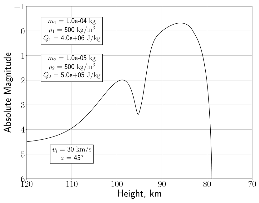
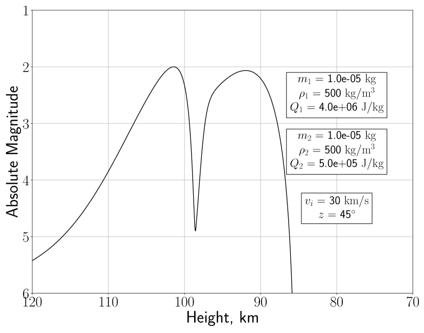
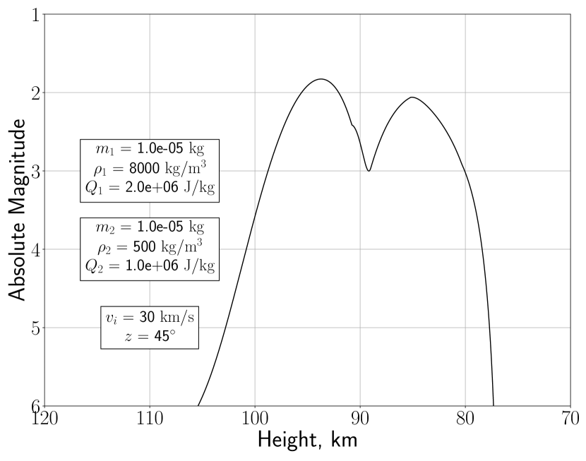
Figure 9: Three simulated meteor events, showing the variety of shapes produced with this ablation model.

We considered the width of the simulated meteors in terms of height (h_begin - h_end), with the beginning and ending heights determined where the absolute magnitudes crossed +4 (this value was selected as many of our observed meteor beginning and/or ending heights are close to that brightness). In our set of 21 studied meteors, the greatest width was 24.6 km, and the average width was 15 km. Of the 71 unique simulated full double peaked meteors, 53 had meteor widths between 5 - 25 km, at magnitudes brighter than +4. Forty-four of the fifty-three simulated meteors had one peak entirely fainter than +4, and the calculated width corresponded to the width of a single peak only (these 44 simulated events thus do not correspond our observations). Ignoring the fact that most of the simulated events have a peak that is fainter than we could confidently observe with our system, we found that none of the fifty-three simulated meteors with widths that agreed with our observations showed shapes that match our observations: the simulated trough is often too sharp, and the simulated rising and falling slopes of the peaks are often too steep.

We looked closely at the simulated double peaked events, in particular, the heats of ablation and density values needed to produce these shapes. These parameters, along with mass, cause the greatest changes in the simulated light curve shape, and are responsible for the observed double peaks. In Fig. 10, we plot the unique meteor events that produced double peaked curves, in terms of the ratio of densities vs the ratio of heats of ablation, separated by the ratio of masses.

The lack of simulated events showing double peaked light curves with a mass ratio of 100 is explained by the fact that with a large mass ratio, one peak (created by the less massive component) will be overshadowed by the other peak (created by the more massive component). Simulated events with a mass ratio of 10 show more double peaked curves than the other two mass ratio options, likely because one component is able to ablate completely before the other, which produces the dip in luminosity (and the mass ratio is low enough that the less massive component is visible). For simulated events with a mass ratio of 1, the two components are possibly ablating at the same time, but the differing compositions may allow double peaks to be produced. Many of the simulated events in this group (mass ratio of 1) are not truly double peaked and look similar to the simulated event shown in Fig. 14. The varying frequency of simulated double peaked events at various density and heat of ablation ratios, for the different mass ratios, indicates that the meteoroid densities and heats of ablation could be important for producing double peaked light curves.

To investigate the role that heat of ablation and density play in producing double peaked meteor light curves, we kept all other values constant and varied heat of ablation or density for the second component through the full range of values. We also investigated the effect of the meteor zenith angle. These results are shown in Fig. 11 and 12.

The effect of the zenith angle is shown in Fig. 13, as well as in Figures 11 and 12. The zenith angle can change the shape of the first peak, shape of the second peak, depth of the trough, brightness of the event, and the beginning and ending heights. The mean zenith angle for our twenty-one events is 33.3^∘: for our simulated meteors we used 45^∘.

Many of the half double peaked (in which either the first peak to trough or trough to second peak is at least 0.5 mag) simulated meteors are actually not double peaked – they show a small hook (Fig. 14), which passes the requirement for one magnitude difference of at least 0.5 mag, but visually fails as a double peaked meteor. The second peak in Fig. 14 would be lost in the noise of the system. This explains the large number of red plus symbols (+) in Fig. 10.

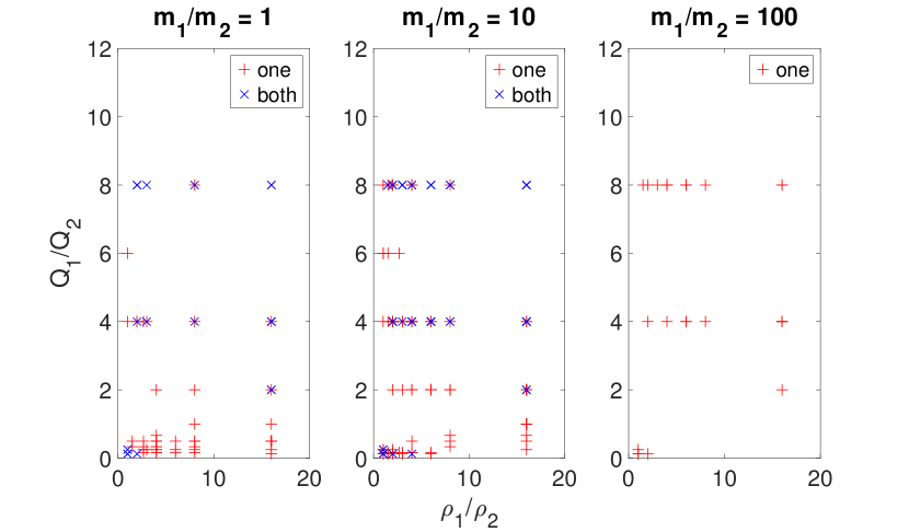
Figure 10: Each plot shows the ratio of heats of ablation versus the ratio of meteoroid densities, for the three possible mass ratios. The red plus symbols (+) indicate simulations which produced a double peaked meteor in which only a single magnitude difference (either the first peak to trough, or the trough to second peak) was greater than 0.5 magnitude (a "half double peak"). The blue crosses (x) indicate simulations in which both magnitude differences were at least 0.5 mag (a "full double peak"). The meteors in these simulations had entry speeds of 30 km/s and zenith angles of 45^∘.

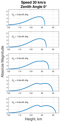
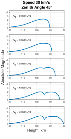
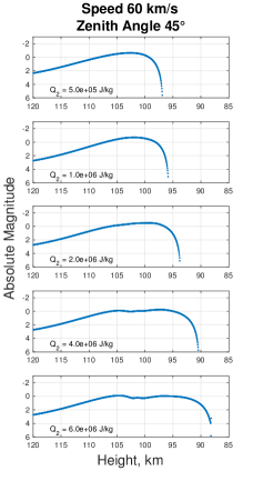
Figure 11: Three figures showing the effect of entry speed, zenith angle, and heat of ablation. The leftmost figure shows (from the top down) the effect of increasing the heat of ablation value for one component in our two-component single body ablation model, for a meteor with an entry speed of 30 km/s and zenith angle of 0^∘. The middle figure shows the same effect, but for a zenith angle of 45^∘. The rightmost figure shows the results for an entry speed of 60 km/s and zenith angle of 45^∘. The parameters for each set of figures were: both component masses were 10^-5kg; both component densities were 1000 kg/m³; and one heat of ablation was 5 X 10⁵ J/kg.

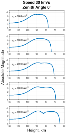
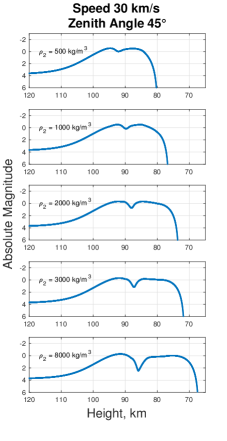
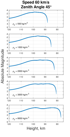
Figure 12: Three figures showing the effect of entry speed, zenith angle, and meteoroid density. The leftmost figure shows (from the top down) the effect of increasing the density value for one component in our two-component single body ablation model, for a meteor with an entry speed of 30 km/s and zenith angle of 0^∘. The middle figure shows the same effect, but for a zenith angle of 45^∘. The rightmost figure shows the results for an entry speed of 60 km/s and zenith angle of 45^∘. The parameters for each set of figures were: both component masses were 10^-4kg; one component density was 500 kg/m³; the heats of ablation were 5 X 10⁵ J/kg and 4 X 10⁶ J/kg.

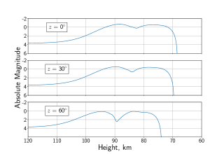
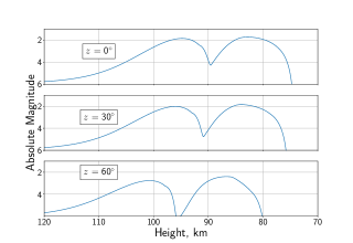
Figure 13: The effect of zenith angle on simulated meteor light curve shape. The meteors for both the left and right figures have the following properties: $\rho_{1}$ = 500 kg/m³; $\rho_{2}$ = 8000 kg/m³; Q₁ = 5 X 10⁵ J/kg; Q₂ = 2 X 10⁶ J/kg. The left figure has m₁ = m₂ = 10^-4 kg. The figure on the right has m₁ = m₂ = 10^-5 kg. Entry speed is 30 km/s.

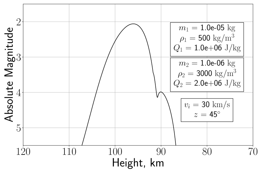
Figure 14: A simulated meteor that was classified as half double peaked, due to the magnitude difference between the first peak and the trough being greater than 0.5 mag. The second ‘peak’ looks more like a blip, and due to noise in the camera system wouldn’t be noticed, and this would be classified as a single peaked light curve.

4.3 Other variations of double peaked curves

The events studied here can be classified into two broad categories, smooth peaked and sudden peaked. There are variations within those groups. Typically, the smooth peaked events show a decrease of half to one magnitude before the next peak begins to increase, as seen in Fig. 2. Some meteor events, however, show a much greater decrease in brightness, as seen in Fig. 15, or an unusual second peak shape, as shown in Fig. 16. Each meteor light curve studied can be found in the Appendix, with their corresponding mirfit brightness profile observations overplotted.

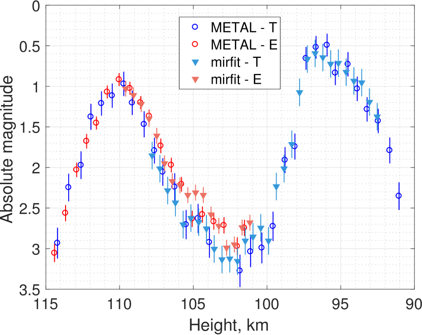
Figure 15: A smoothed peaked meteor light curve showing a greater decrease in brightness than most events, over a greater height range. The second peak was observed exclusively at the Tavistock station. This is meteor event 20111104_0832320.

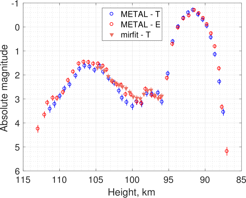
Figure 16: A smoothed peaked meteor light curve (event 20160808_083545)

showing an unusual shape (and possibly a third peak nestled between the two distinct peaks). Only one narrow-field camera tracked this meteor, and it did not observe the second peak.

5 Conclusions

We analysed 21 double peaked meteor light curves and found that five of those meteor events showed ‘sudden peaked’ curves, and the remaining 16 showed ‘smooth peaked’ light curves. The sudden peaked meteor events were on asteroidal orbits, and mostly showed fragmentation, whereas the smooth peaked curves were on cometary orbits and showed mostly faint wake in their narrow-field observations. The difference in origin between the two types of light curve is striking but difficult to explain; the differences in the appearance of the sudden peaked and smooth peaked curves may be related to the composition and structure of the meteoroids. This is particularly interesting in light of the results of Subasinghe et al. (2016), who found no difference in the light curve shapes or fragmentation behaviour between dynamically asteroidal and cometary meteoroids. The sample size here is small, but the near complete separation of the two populations is still suggestive.

The sudden peaked light curves might be explained by a sudden release of grains, as used in the analysis done by Roberts et al. (2014), since many of those meteors showed fragmentation. On the other hand, this burst of fragmentation seems to be an unlikely mechanism for many of the smooth peaked events analysed here, as indicated by the time evolution of the narrow-field observations, which are consistent only with the shedding of small fragments as modelled in Campbell-Brown (2017). Spectral observations were not collected for this study, but will be in the future; those observations will confirm whether differential ablation is occurring, and whether a particular elemental composition is responsible for each peak. Ablation modelling using only inhomogeneous compositions without fragmentation was able to produce double peaked light curves if the two components had densities or heats of ablation which differed by more than a factor of 2, but the width of the light curves tended to be larger than the observed widths, implying that some form of fragmentation must play a role, even when composition is the dominant effect. In the future, ablation modelling of meteor events with double peaked light curves using a two component model that includes fragmentation mechanisms may be attempted to investigate possible mechanisms, and physical properties such as grain sizes and distributions, structure and composition, and mass.

Appendix A Sudden peaked meteor events

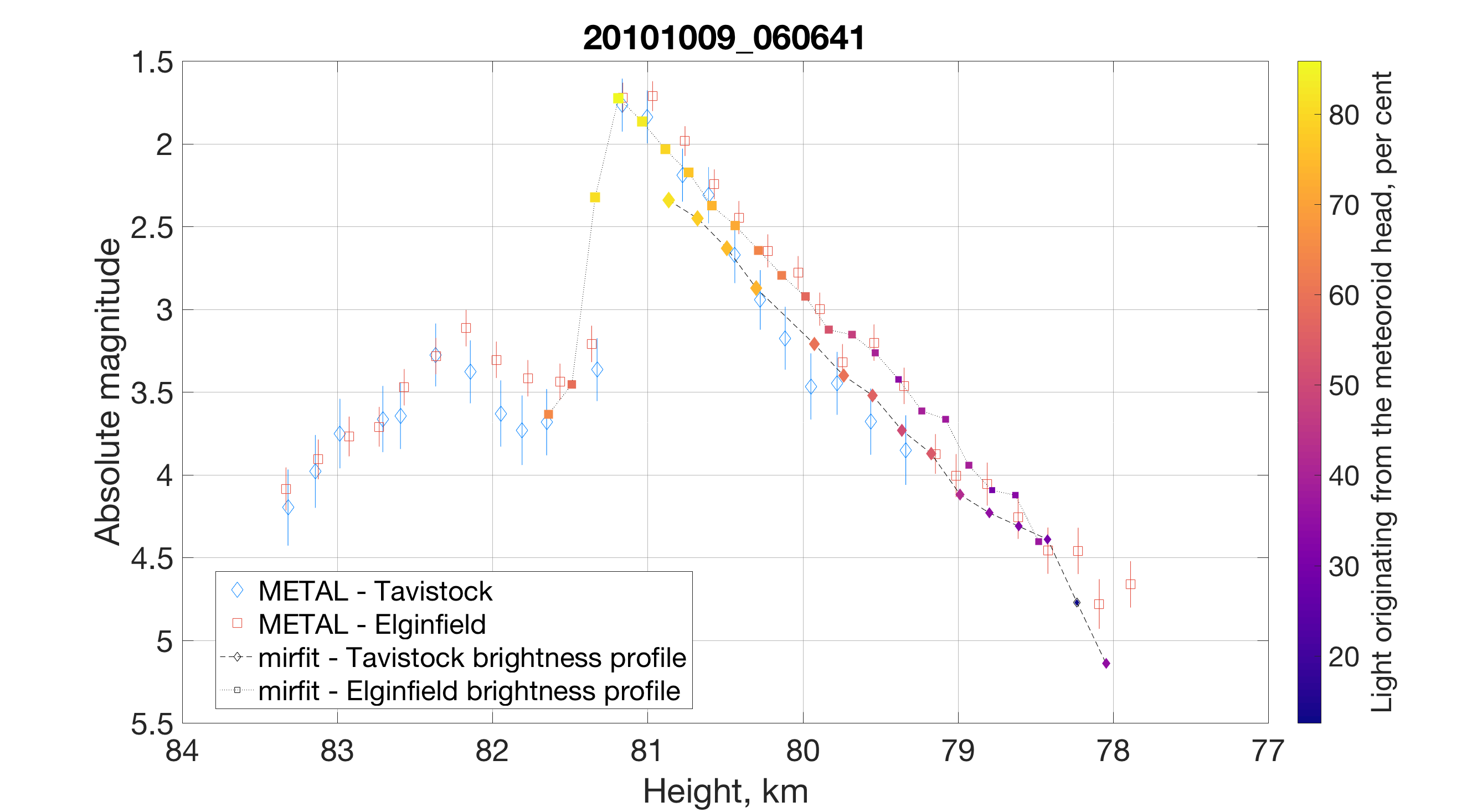
Figure 17: 20101009_060641

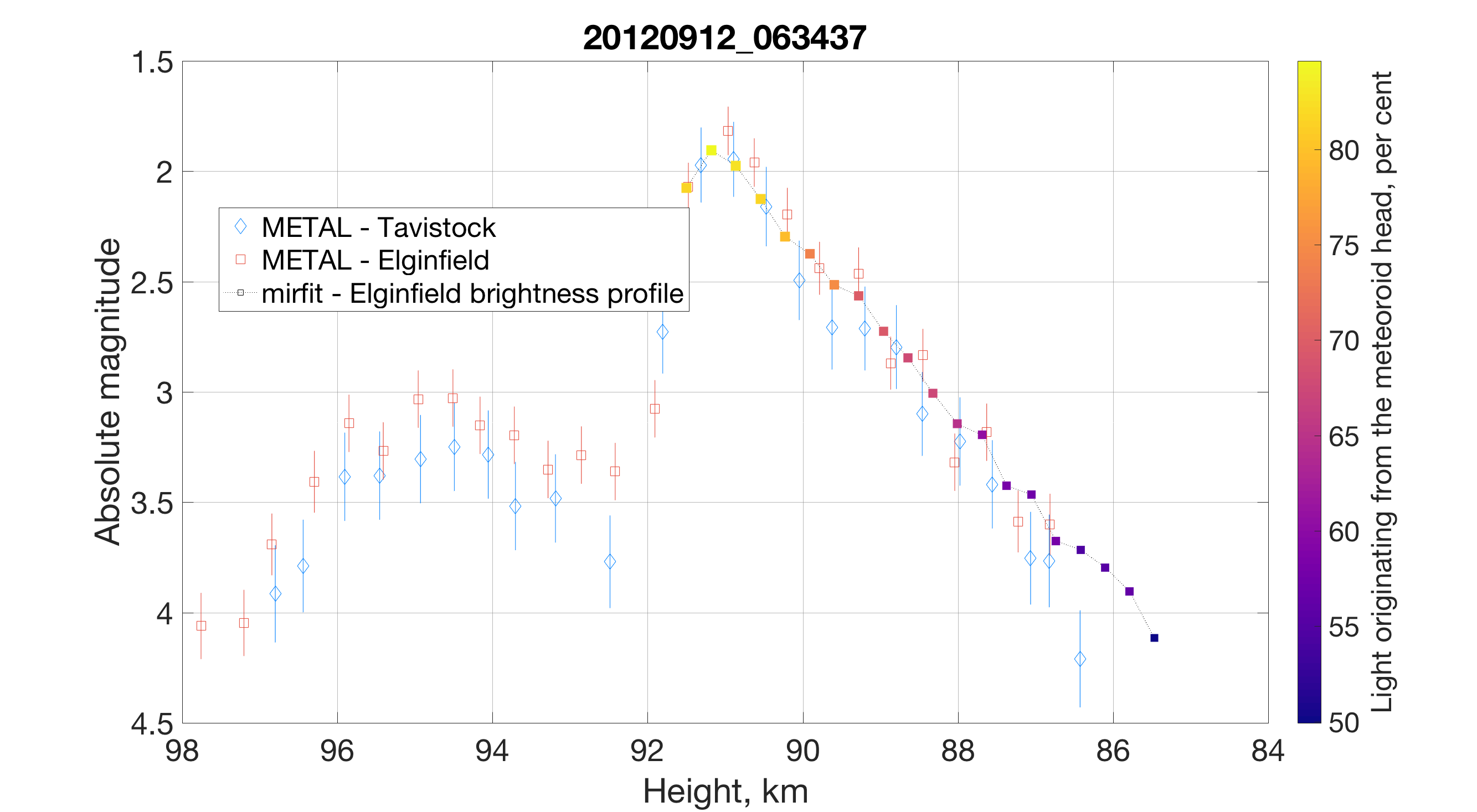
Figure 18: 20120912_063437

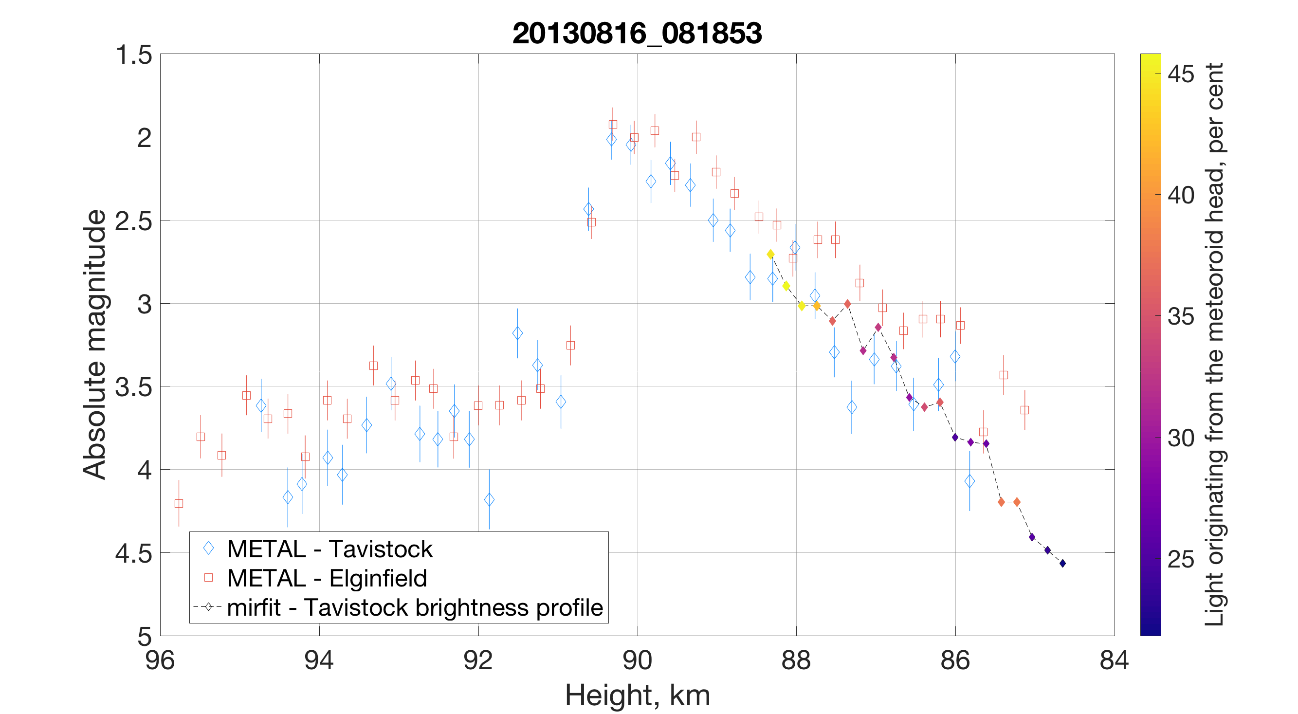
Figure 19: 20130816_081853

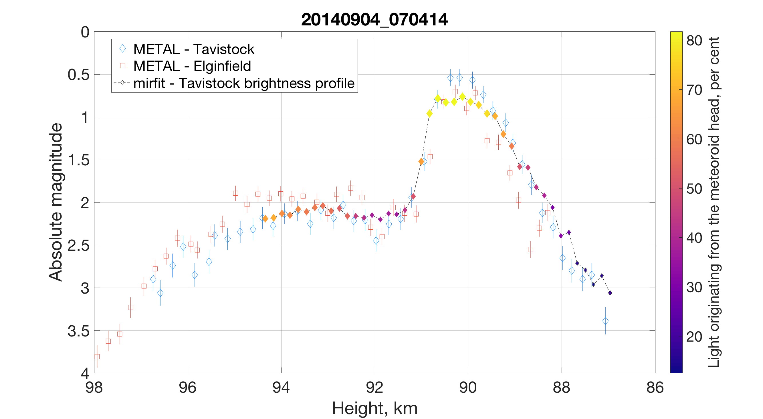
Figure 20: 20140904_070414

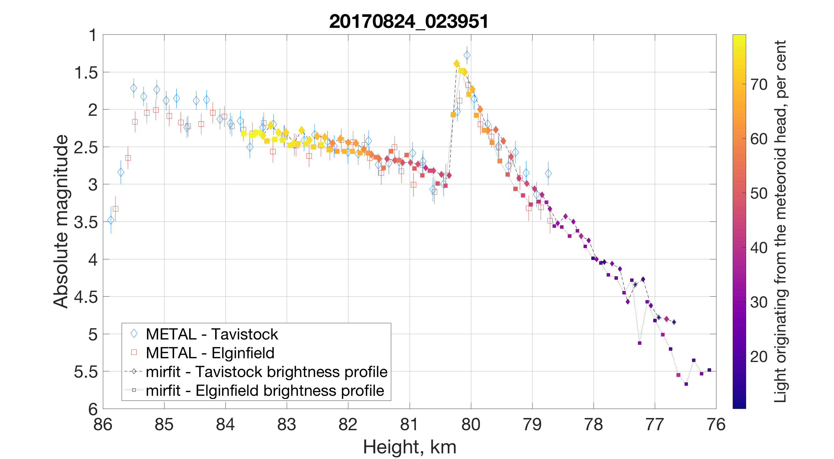
Figure 21: 20170824_023951

Appendix B Smooth peaked meteor events

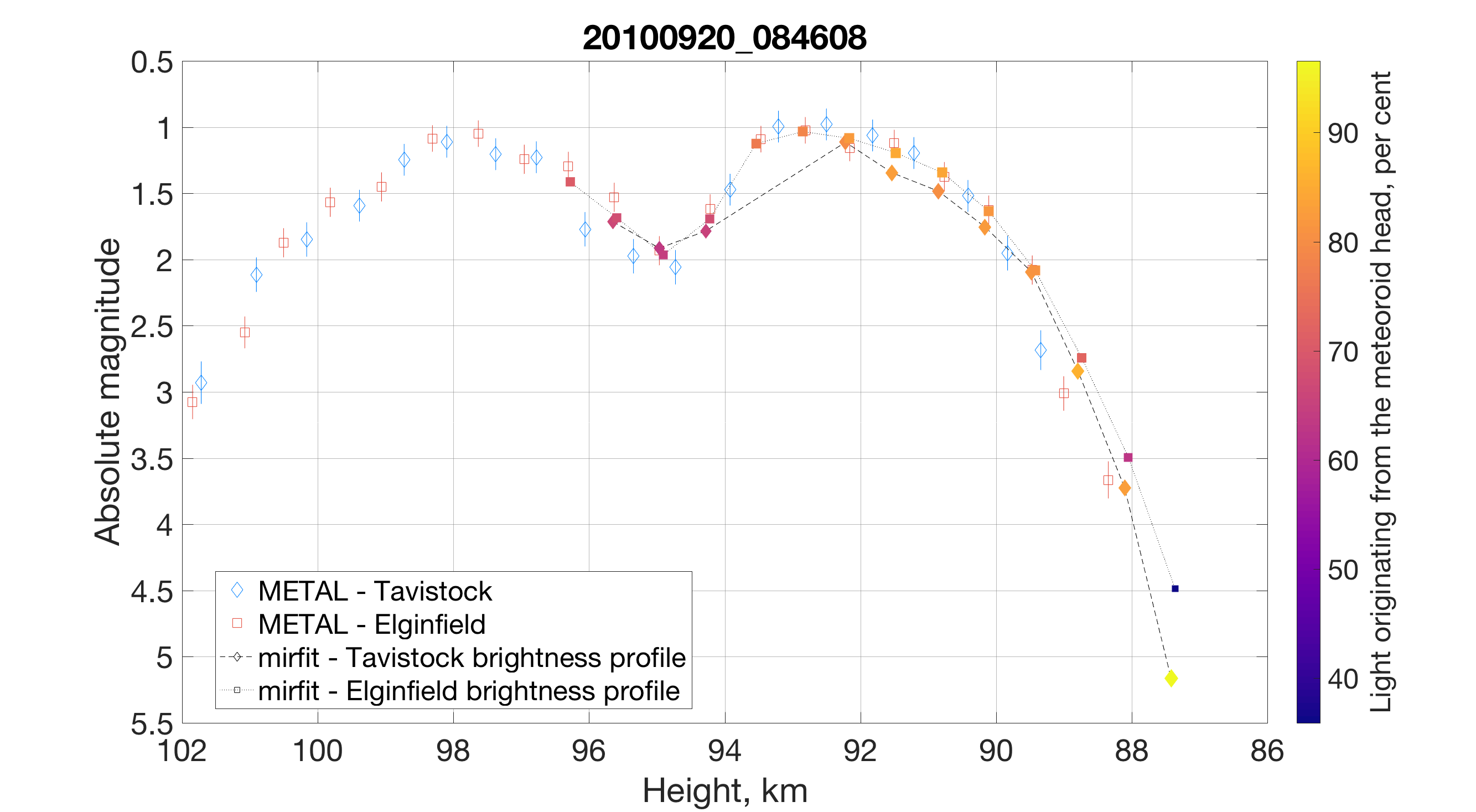
Figure 22: 20100920_084608

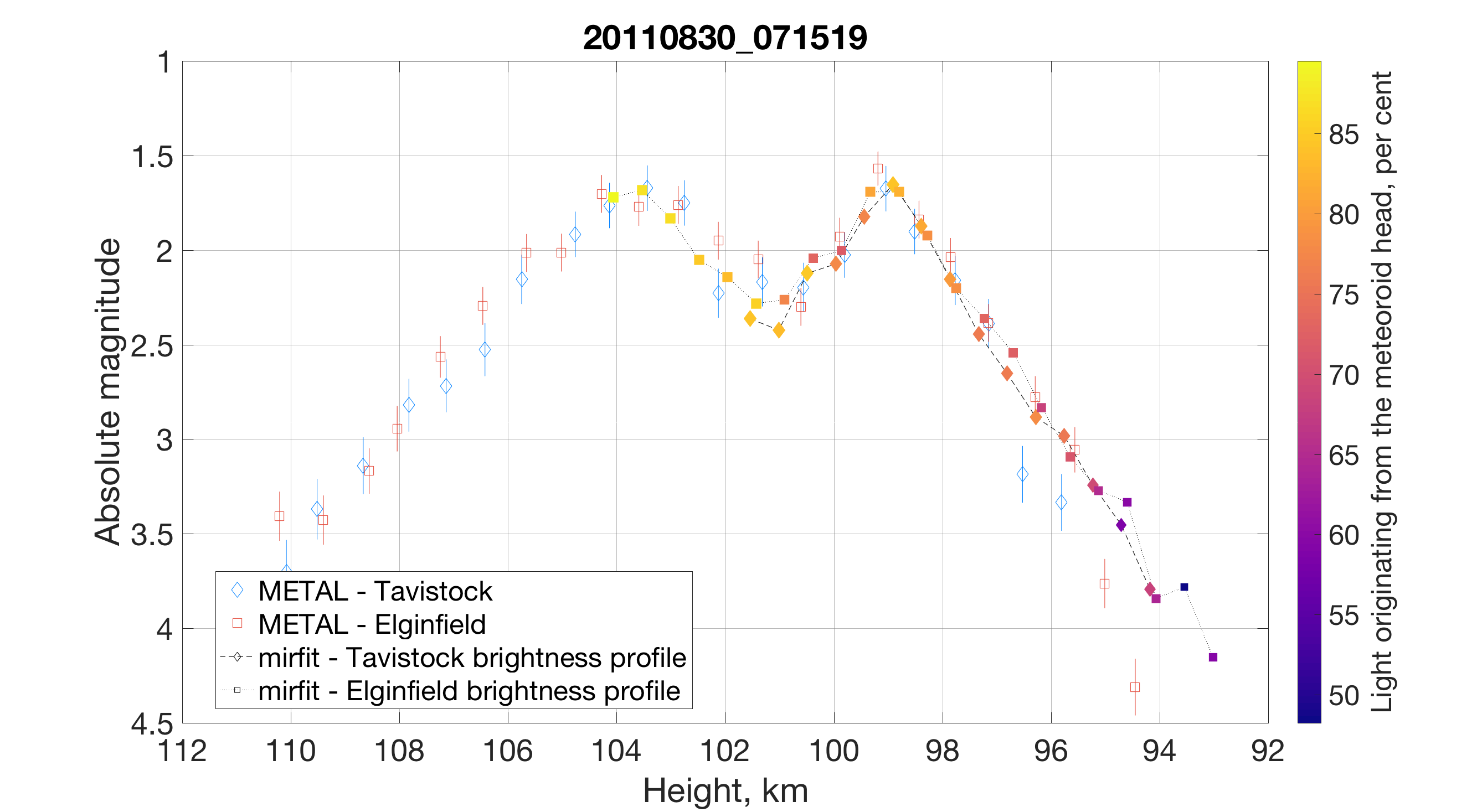
Figure 23: 20110830_071519

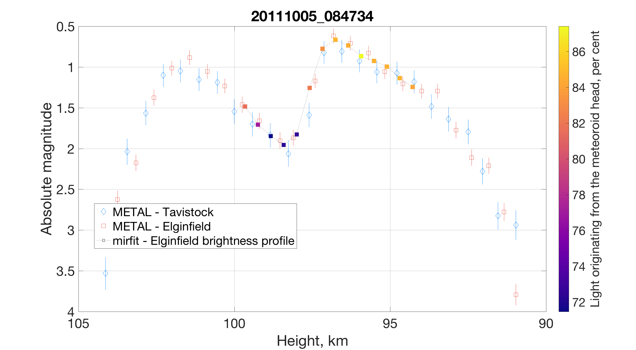
Figure 24: 20111005_084734

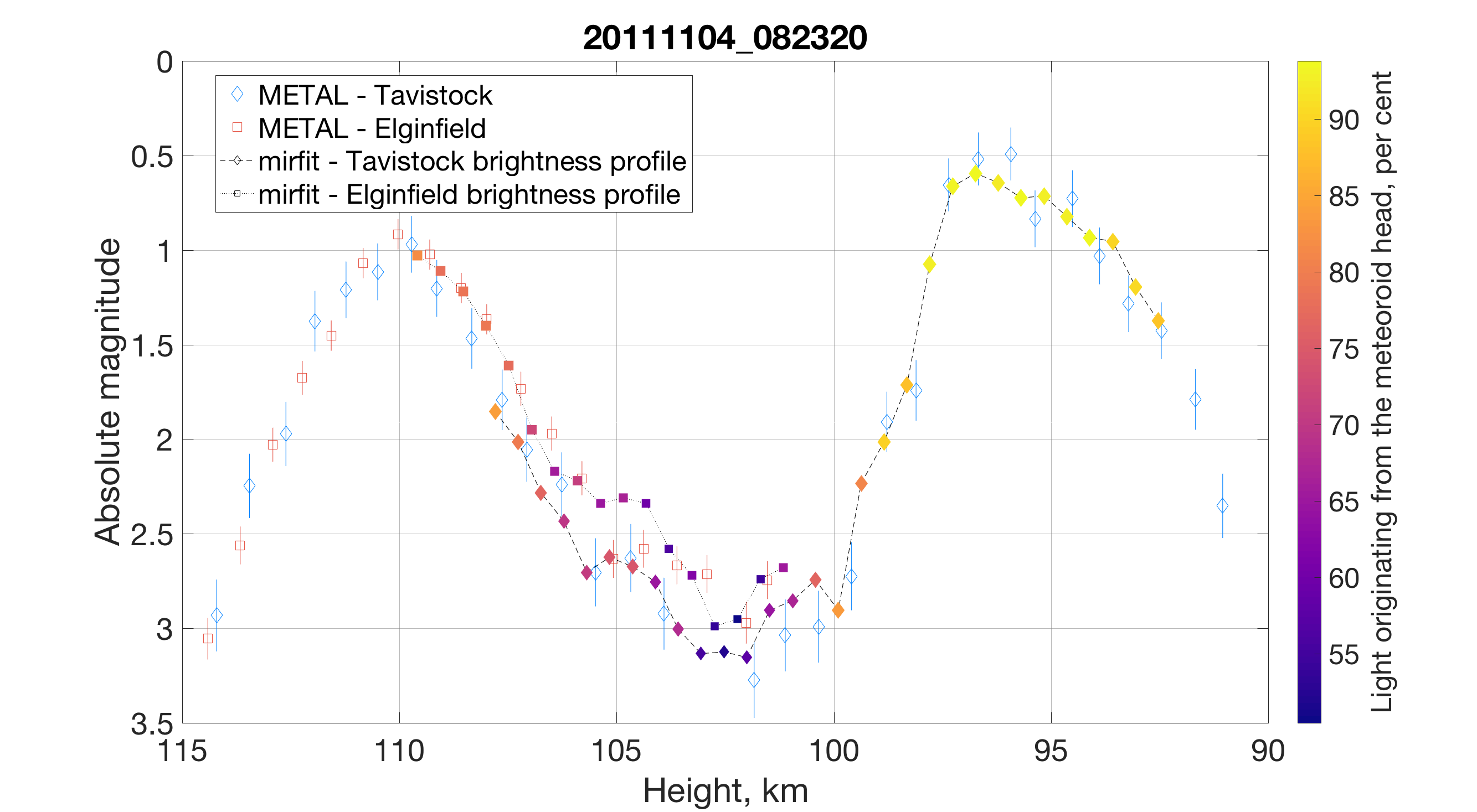
Figure 25: 20111104_082320

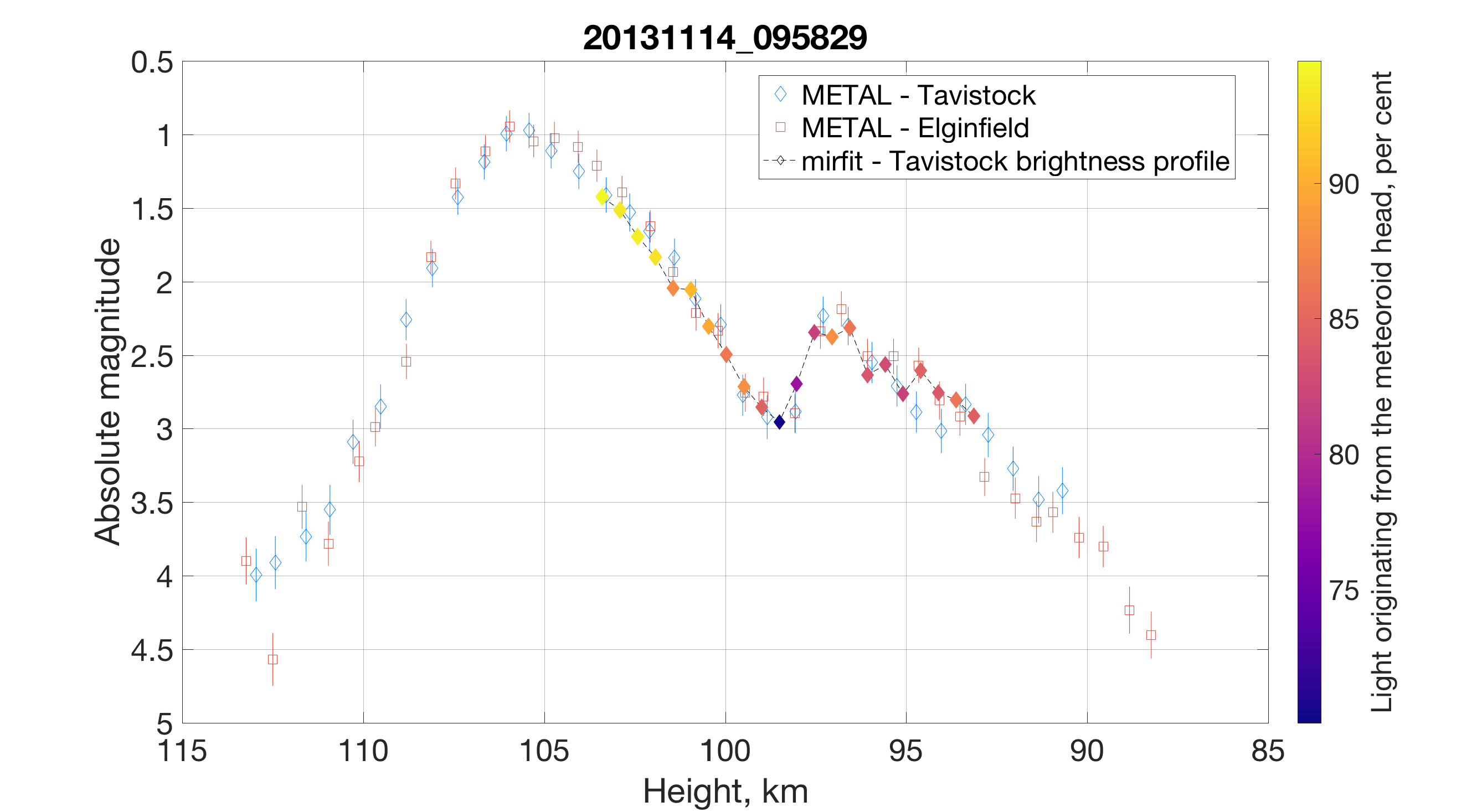
Figure 26: 20131114_095829

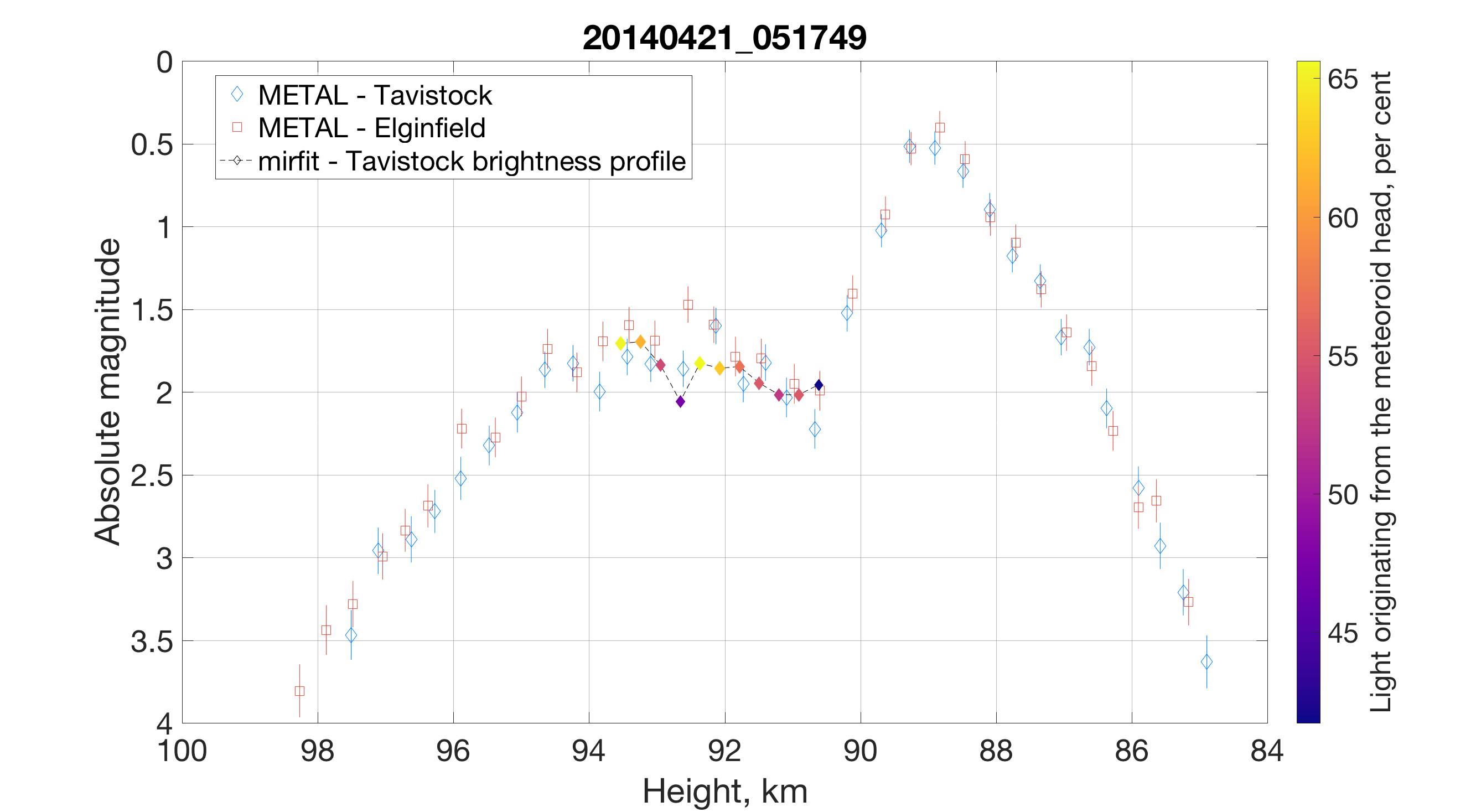
Figure 27: 20140421_051749

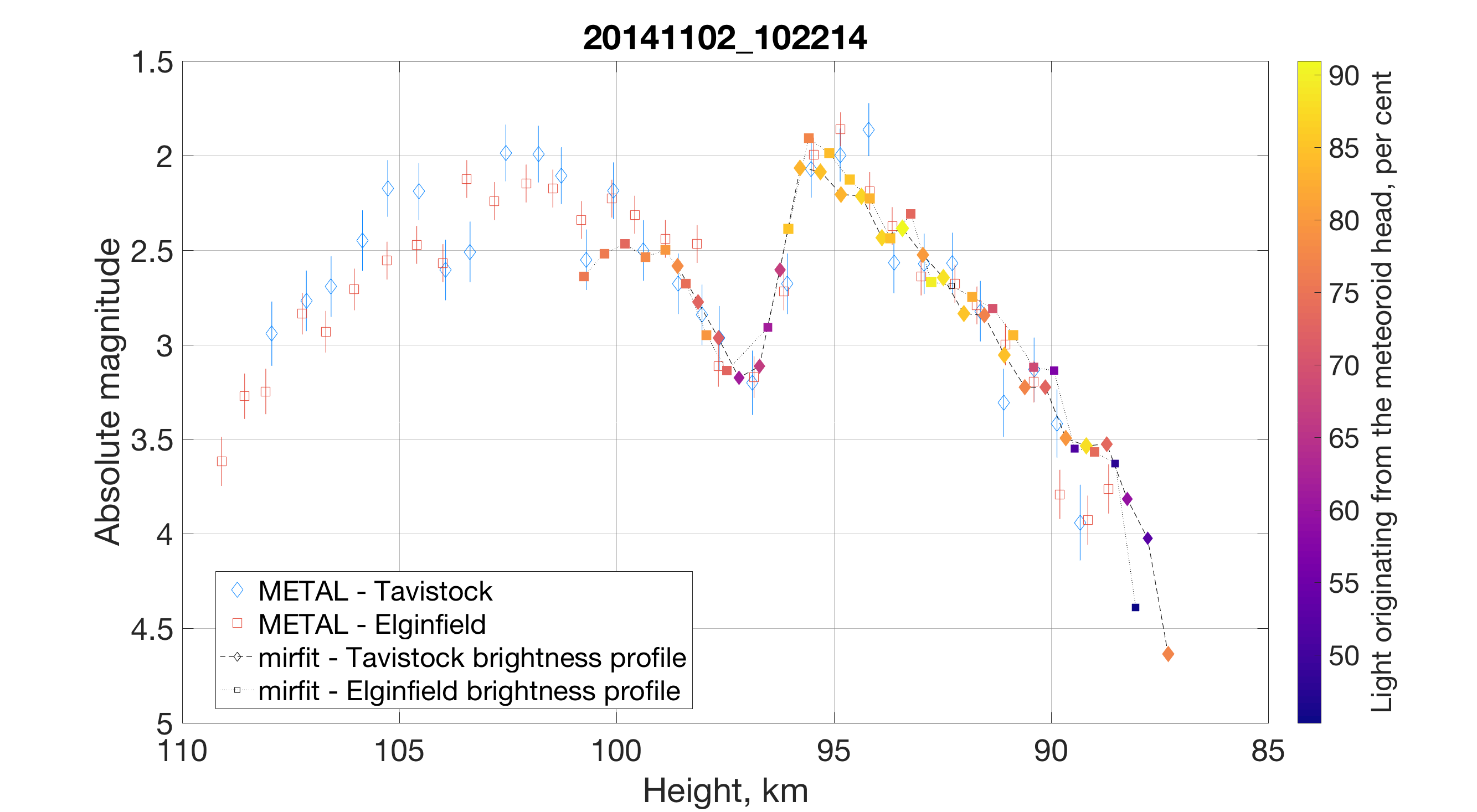
Figure 28: 20141102_102214

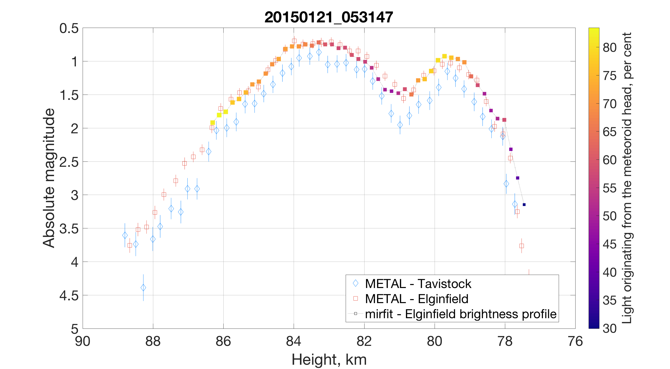
Figure 29: 20150121_053147

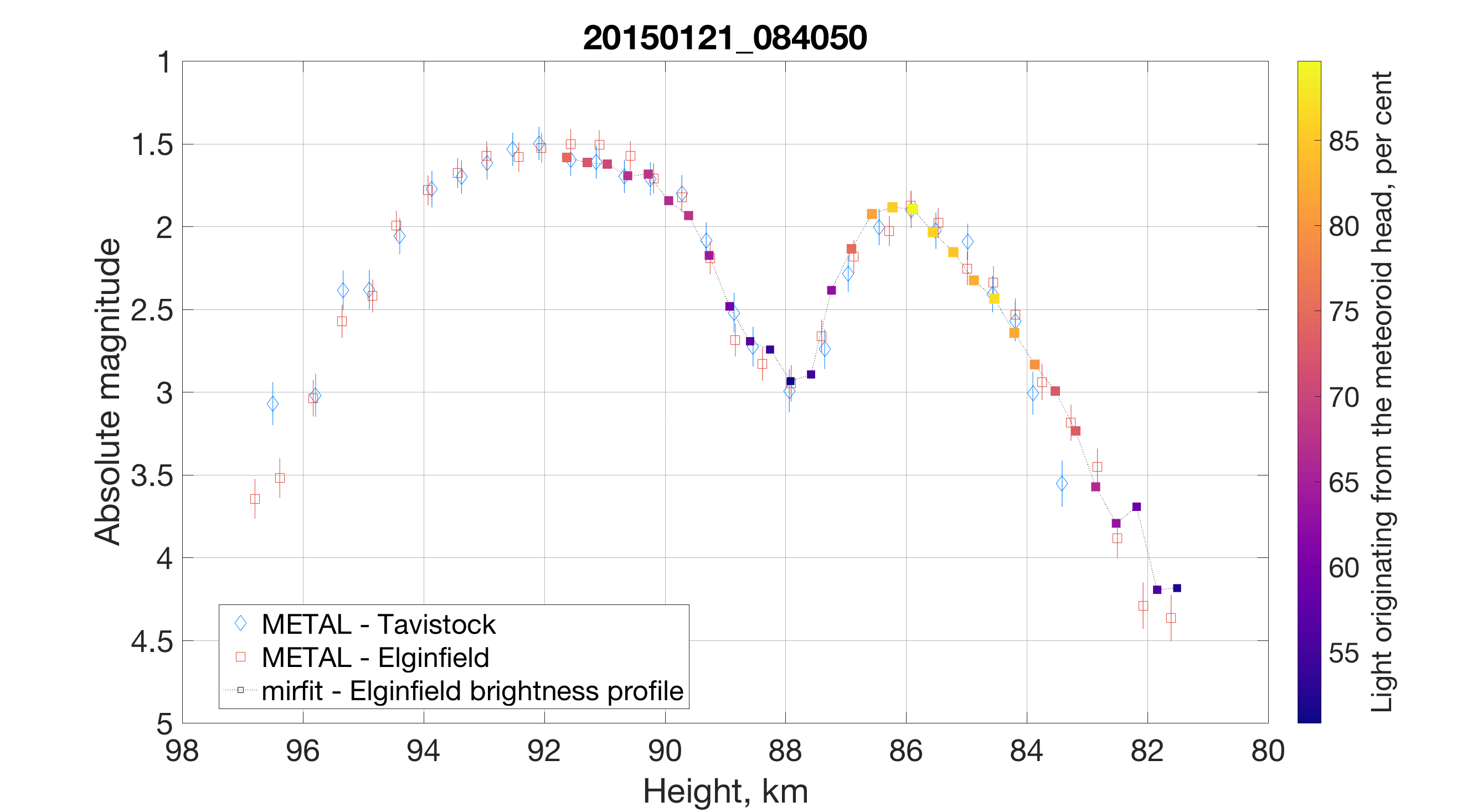
Figure 30: 20150121_084050

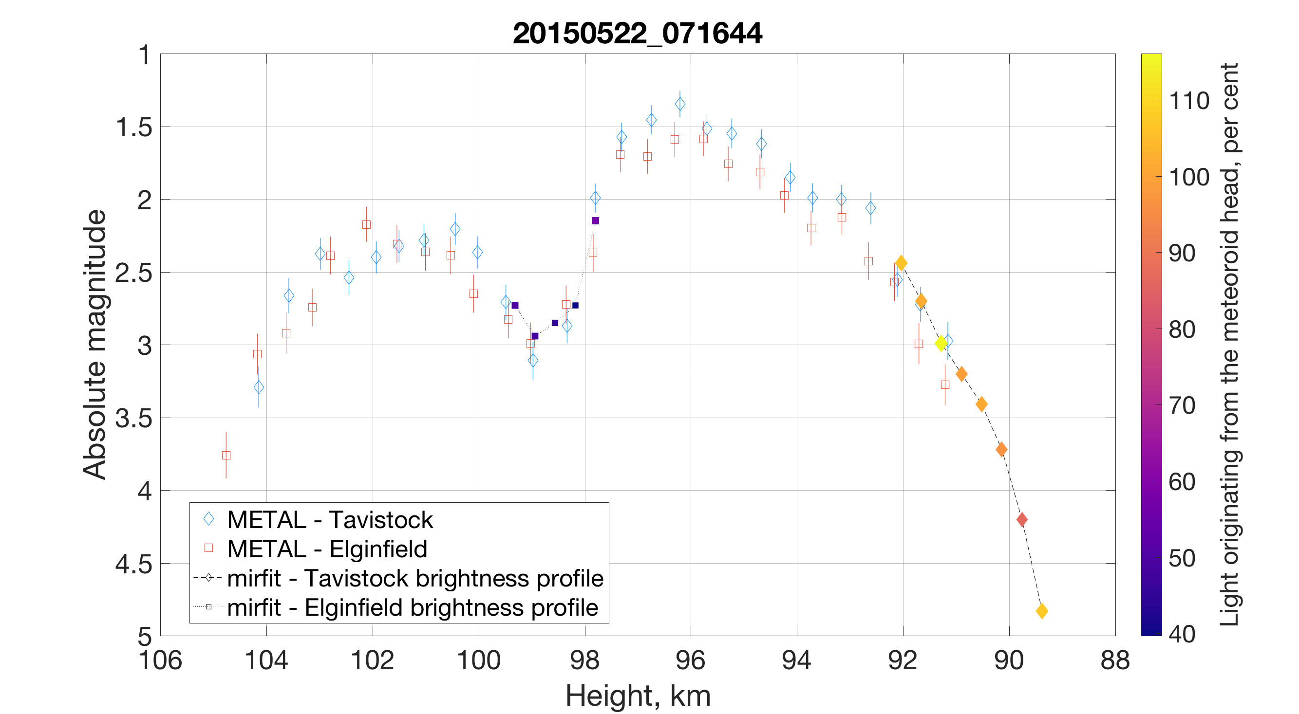
Figure 31: 20150522_071644

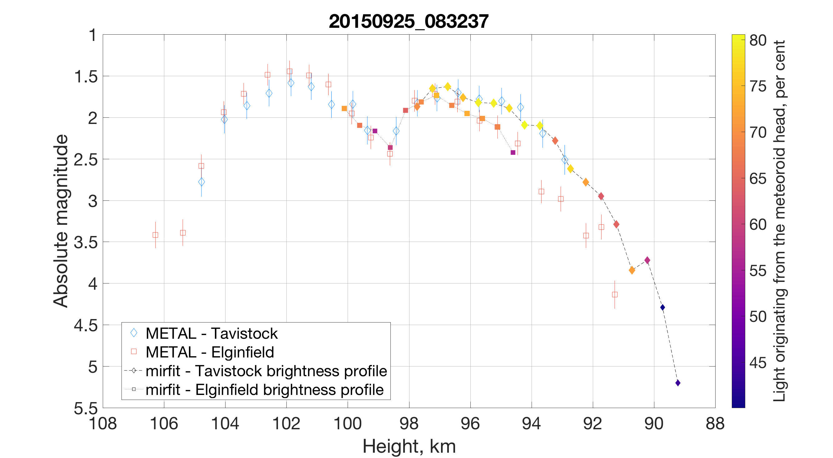
Figure 32: 20150925_083237

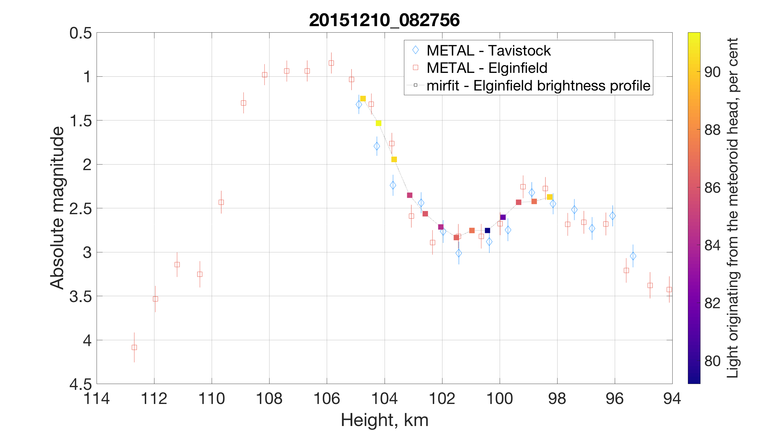
Figure 33: 20151210_082756

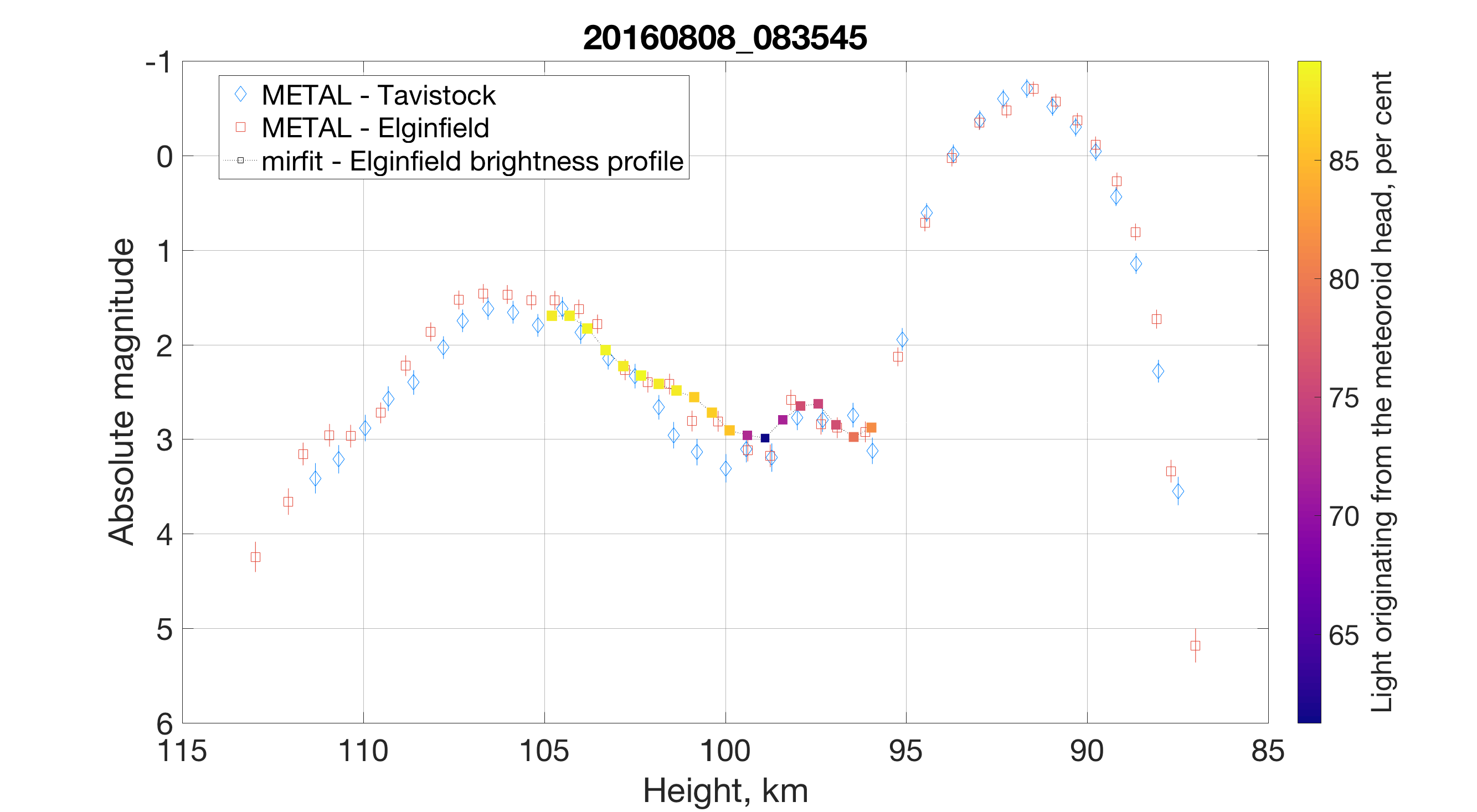
Figure 34: 20160808_083545

Figure 35: 20170924_070328

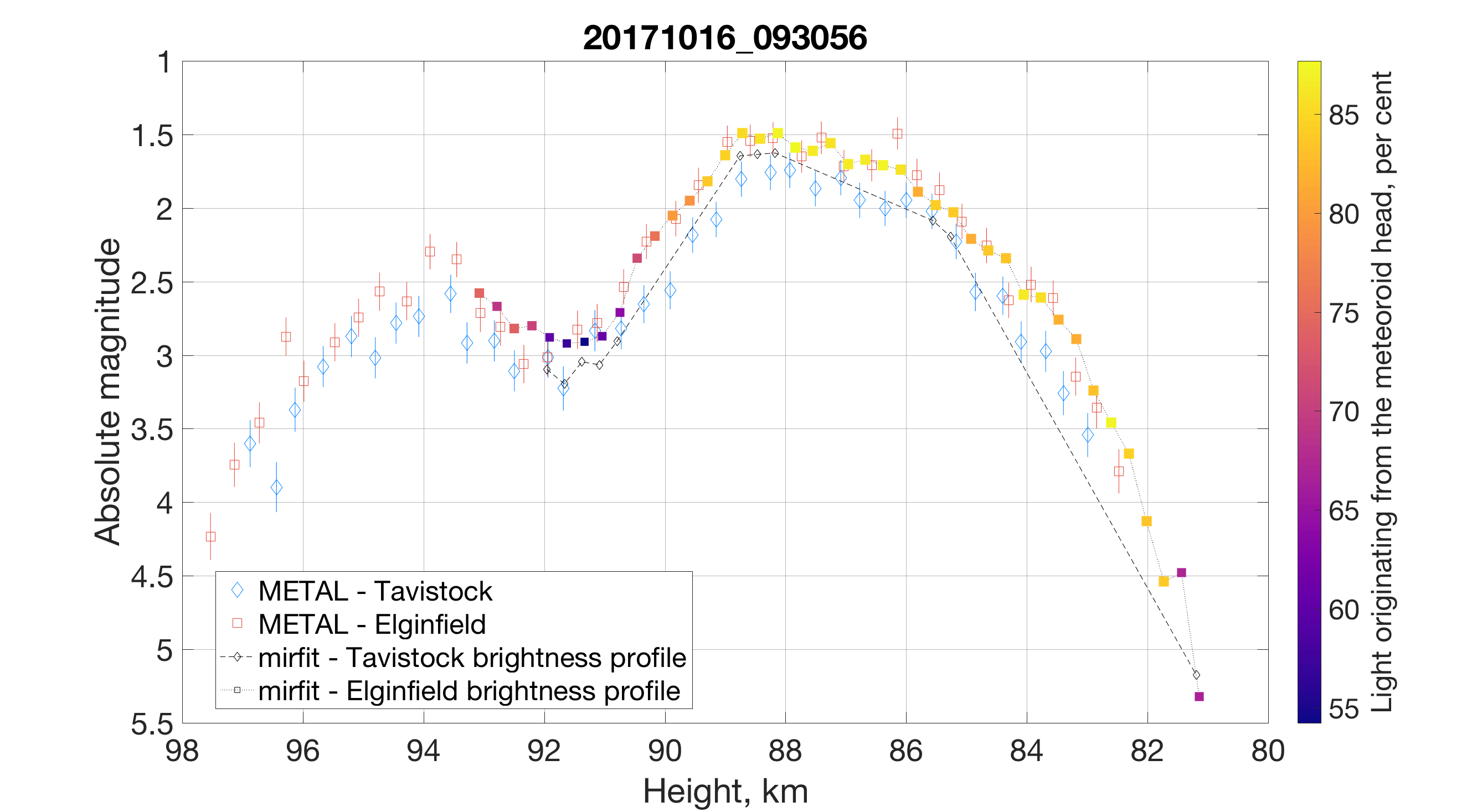
Figure 36: 20171016_093056

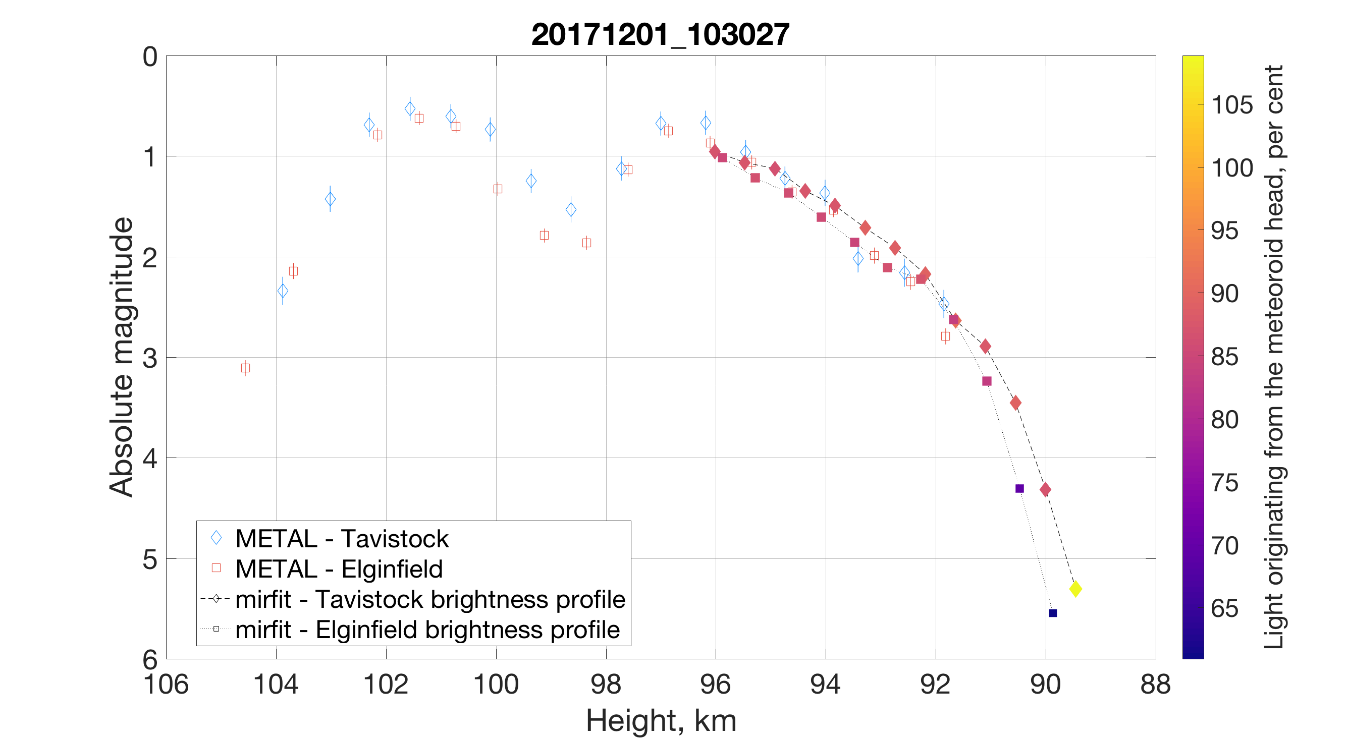
Figure 37: 20171201_103027

References

- Beech & Murray (2003) Beech M., Murray I. S., 2003, Monthly Notices of the Royal Astronomical Society, 345, 696
- Bloxam & Campbell-Brown (2017) Bloxam K., Campbell-Brown M., 2017, Planet. Space Sci., 143, 28
- Borovicka (1990) Borovicka J., 1990, Bull. Astron. Inst. Czechoslovakia, 41, 391
- Borovicka et al. (1999) Borovicka J., Stork R., Bocek J., 1999, Meteoritics and Planetary Science, 34, 987
- Borovička et al. (2007) Borovička J., Spurný P., Koten P., 2007, A&A, 473, 661
- Campbell-Brown (2017) Campbell-Brown M., 2017, Planet. Space Sci., 143, 34
- Campbell-Brown & Koschny (2004) Campbell-Brown M. D., Koschny D., 2004, A&A, 418, 751
- Campbell-Brown et al. (2013) Campbell-Brown M. D., Borovička J., Brown P. G., Stokan E., 2013, Astronomy and Astrophysics, 557, A41
- Ceplecha (1958) Ceplecha Z., 1958, Bulletin of the Astronomical Institutes of Czechoslovakia, 9, 154
- Fleming et al. (1993) Fleming D. E. B., Hawkes R. L., Jones J., 1993, in Stohl J., Williams I. P., eds, Meteoroids and their Parent Bodies. p. 261
- Hawkes & Jones (1975) Hawkes R. L., Jones J., 1975, MNRAS, 173, 339
- Jacchia (1955) Jacchia L. G., 1955, ApJ, 121, 521
- Koten et al. (2004) Koten P., Borovička J., Spurný P., Betlem H., Evans S., 2004, A&A, 428, 683
- Murray et al. (2000) Murray I. S., Beech M., Taylor M. J., Jenniskens P., Hawkes R. L., 2000, Earth Moon and Planets, 82, 351
- Myers et al. (2001) Myers J. R., Sande C. B., Miller A. C., Warren Jr. W. H., Tracewell D. A., 2001, VizieR Online Data Catalog, 5109
- Roberts (2014) Roberts I. D., 2014, Simulation of Double Peaked Meteor Light Curves, Thesis
- Roberts et al. (2014) Roberts I. D., Hawkes R. L., Weryk R. J., Campbell-Brown M. D., Brown P. G., Stokan E., Subasinghe D., 2014, Meteoroids 2013,
- Schneider et al. (2012) Schneider C. A., Rasband W. S., Eliceiri K. W., 2012, Nat Meth, 9, 671
- Subasinghe et al. (2016) Subasinghe D., Campbell-Brown M. D., Stokan E., 2016, MNRAS, 457, 1289
- Verniani (1965) Verniani F., 1965, Smithsonian Contributions to Astrophysics, 8, 141
- Wasson & Rubin (2010) Wasson J. T., Rubin A. E., 2010, Geochimica Cosmochimica Acta, 74, 2212
- Weryk & Brown (2012) Weryk R. J., Brown P. G., 2012, Planet. Space Sci., 62, 132
- Weryk et al. (2013) Weryk R. J., Campbell-Brown M. D., Wiegert P. A., Brown P. G., Krzeminski Z., Musci R., 2013, Icarus, 225, 614
- Wood (1963) Wood J. A., 1963, Icarus, 2, 152