Cosmic Evolution of Holographic Dark Energy in $f(\mathcal{G},T)$ Gravity

Abstract

The aim of this paper is to analyze the cosmological evolution of holographic dark energy in $f(\mathcal{G},T)$ gravity ($\mathcal{G}$ and $T$ represent the Gauss-Bonnet invariant and trace of the energy-momentum tensor, respectively). We reconstruct $f(\mathcal{G},T)$ model through correspondence scheme using power-law form of the scale factor. The qualitative analysis of the derived model is investigated with the help of evolutionary trajectories of equation of state, deceleration as well as state-finder diagnostic parameters and $\omega_{{}_{\mathcal{G}T}}-{\omega}^{\prime}_{{}_{\mathcal{G}T}}$ cosmological phase plane. It is found that the equation of state parameter represents phantom epoch of the Universe whereas the deceleration parameter illustrates the accelerated phase. The state-finder plane corresponds to Chaplygin gas model while the freezing region is attained in $\omega_{{}_{\mathcal{G}T}}-{\omega}^{\prime}_{{}_{\mathcal{G}T}}$ plane.

Keywords: Dark energy; $f(\mathcal{G},T)$ gravity.
PACS: 04.50.Kd; 95.36.+x.

1 Introduction

The surprising discovery of the accelerated expansion of the Universe is one of the exciting progress in cosmology. This tremendous change in cosmic history has been proved from a diverse set of high-precision observational data accumulated from various astronomical sources. The accelerating paradigm is considered as a consequence of an exotic type of force dubbed as dark energy (DE) which possesses repulsive characteristics with negatively large pressure. It may predict the ultimate future of the Universe but its salient features are still not known. To explore the perplexing nature of DE, different approaches have been presented. The cosmological constant $(\Lambda)$ is the simplest approach while modified theories of gravity and dynamical DE models have also been proposed in this regard. The cosmological constant suffers from problems like fine tuning (large discrepancy between its theoretical predicted and observed value) and coincidence between the observed vacuum energy and the current matter density. Modified gravitational theories act as an alternative for dark energy (DE) and are obtained by replacing or adding curvature invariants as well as their corresponding generic functions in the geometric part of the Einstein-Hilbert action. It is found that the negative powers of scalar curvature $(R)$ in $f(R)$ theory act as an alternative to DE and thus produce acceleration in the cosmic expansion while its positive powers elegantly describe the inflationary era [1]. Various modified theories possess quite rich cosmological structure, pass the solar system constraints, efficiently describe the bouncing cosmology as well as provide a gravitational alternative for a unified description of the inflationary epoch to the late-time accelerated expansion [2]-[6].

Gauss-Bonnet (GB) invariant being a particular linear combination of quadratic curvature invariants has gained much attention in cosmology. This four-dimensional topological invariant is free from spin-2 ghost instabilities and is defined as [7]-[9]

$$\mathcal{G}=R^{2}-4R_{\xi\eta}R^{\xi\eta}+R_{\xi\eta\mu\nu}R^{\xi\eta\mu\nu},$$ (1)

where $R_{\xi\eta}$ and $R_{\xi\eta\mu\nu}$ are the Ricci and Riemann tensors, respectively. To investigate the dynamics of $\mathcal{G}$ in four dimensions, Nojiri et al. [10] coupled the GB invariant with scalar field and demonstrated that the cosmic accelerated expansion may be produced by the mixture of scalar phantom and/or potential/stringy effects while this scalar GB coupling acts against the big-rip occurrence in phantom cosmology. Without the presence of scalar field, Nojiri and Odintsov [11] presented $f(\mathcal{G})$ gravity as an alternative for DE by adding generic function $f(\mathcal{G})$ in the Einstein-Hilbert action. This theory elegantly describes the fascinating characteristics of late-time cosmological evolution as well as consistent with solar system constraints for a wide range of cosmological viable model parameters [12, 13]. Bamba et al. [14] investigated the finite-time future singularities and found a possible way to cure these singularities in $f(\mathcal{G})$ as well as $f(R,\mathcal{G})$ theories of gravity. Odintsov et al. [15] discussed the super-bounce and loop quantum ekpyrotic cosmologies in the context of modified gravitational theories.

The non-minimal curvature-matter coupling in modified gravitational theories has gained significant attention, since it can describe consistently the late-time acceleration phenomenon. Harko et al. [16] proposed $f(R,T)$ theory of gravity as a generalization of $f(R)$ gravity such that it involves the non-minimal coupling between $R$ and $T$. Recently, we introduced such coupling in $f(\mathcal{G})$ gravity referred as $f(\mathcal{G},T)$ theory and found that the covariant divergence of energy-momentum tensor is not zero [17]. An extra force is appeared as a consequence of this non-zero divergence due to which the non-geodesic trajectories are followed by massive test particles while test particles with zero pressure move along geodesic lines of geometry. The stability of Einstein Universe against homogeneous isotropic and anisotropic scalar perturbations is analyzed for both conserved as well as non-conserved energy-momentum tensor in this theory and found stable results [18, 19]. Shamir and Ahmad [20] constructed some cosmological viable $f(\mathcal{G},T)$ model using Noether symmetry approach in the context of homogeneous and isotropic Universe. The background of cosmic evolutionary models corresponding to de Sitter Universe, power-law solution as well as phantom/non-phantom epochs can be reproduced in this theory [21].

Dynamical DE models have been constructed in the framework of general relativity and quantum gravity which play an important role to explore the mystery of cosmic expansion. Li [22] proposed holographic DE in the background of quantum gravity using the basic concept of holographic principle which stands on the unified pillars of quantum mechanics and gravity. This principle has gained much importance by investigating quantum properties of black holes and stimulated the attention of many researchers to explore string theory or quantum gravity [23]. Cohen et al. [24] reconciled Bekenstein’s entropy bound by establishing a relationship between ultraviolet and infrared cutoffs due to the limit made by the black hole formation. In other words, the total energy of a system with size $L$ should not be greater than the mass of black hole with the same size for the quantum zero-point energy density associated with the ultraviolet cutoff. This leads to the inequality $L^{3}\rho_{{}_{\Lambda}}\leq LM_{{}_{P}}^{2}$, where $M_{{}_{P}}^{2}=(8\pi G)^{-1}$ ($G$ is the gravitational constant), $L$ and $\rho_{{}_{\Lambda}}$ are the reduced Planck mass, infrared cutoff and energy density of holographic DE, respectively.

The accelerated expansion of the Universe is also successfully discussed in literature via correspondence scheme of dynamical DE models with modified theories of gravity. In this mechanism, generic function of the considered gravity is reconstructed by comparing the corresponding energy densities. A variety of reconstructed holographic DE models in different modified theories have gained remarkable importance in describing the present cosmic phase. Setare [25] examined the cosmological evolution of holographic DE in $f(R)$ gravity for the flat FRW Universe model and found that the reconstructed model behaves like phantom epoch of DE dominated era. Setare and Saridakis [26] developed a correspondence between holographic DE scenario in flat FRW Universe and phantom DE model in GB gravity coupled with a scalar field and found that this correspondence consistently leads to the cosmic accelerated expansion. Karami and Khaledian [27] reconstructed the new agegraphic as well as holographic DE $f(R)$ models for both ordinary as well as entropy corrected version in flat FRW Universe model. They found that both ordinary models behave like phantom or non-phantom while the entropy corrected reconstructed models experience the phase transition from quintessence to phantom epochs of the Universe.

Houndjo and Piattella [28] reconstructed holographic DE $f(R,T)$ model numerically and observed that the same cosmic history may be discussed by holographic DE model as in general relativity. Daouda and his collaborators [29] formulated the holographic DE model in generalized teleparallel theory and concluded that the resultant model implies unified mechanism of dark matter with DE. Jawad et al. [30] analyzed the stability of this dynamical DE model with Granda-Oliveros cutoff in $f(\mathcal{G})$ gravity using emergent, intermediate as well as logamediate scale factor and found that the derived model is stable only for the intermediate case. Sharif and Zubair [31] investigated the holographic as well as new agegraphic DE model in $f(R,T)$ gravity and observed that the reconstructed models can demonstrate the phantom or quintessence phases. They also discussed the generalized second law of thermodynamics for the derived models and established the viability conditions. Fayaz et al. [32] found that the reconstructed $f(R,T)$ models corresponding to holographic as well as new ageagraphic DE in the context of Bianchi type I Universe model illustrate phantom or quintessence regions.

In curvature-matter coupled gravitational theories, various dynamical DE models have also gained significant importance in describing the cosmic evolutionary phases. Sharif and Zubair [33] considered the Ricci and modified Ricci DE models to establish the equivalence between these dynamical DE models and $f(R,T)$ gravity via reconstruction technique. They discussed the Dolgov-Kawasaki instability criteria to explore the viability of reconstructed models and found that the appropriate choice of parameters in explaining the evolution of $f(R,T)$ models is consistent with the viability conditions. Zubair and Abbas [34] reconstructed the $f(R,T)$ theory for modified as well as Garcia-Salcedo ghost DE models and analyzed the stability of reconstructed ghost $f(R,T)$ models in the background of flat FRW Universe model. They found that reconstructed ghost models elegantly describe the phantom and quintessence regimes of the Universe. Fayaz et al. [35] studied the anisotropic Universe with ghost DE model and found that the reconstructed $f(R,T)$ models can reproduce the cosmic phantom epoch satisfying the current observations. Baffou and his collaborators [36] investigated the generalized Chaplygin gas interacting with $f(R,T)$ theory of gravity in the presence of bulk as well as shear viscosities and found that the viscous parameters are well accommodated with observational data. Zubair et al. [37] explored the cosmic evolution of $f(R,T)$ gravity in the presence of matter fluids consisting of radiation as well as collisional self-interacting dark matter. Tiwari et al. [38] constructed the cosmological model with variable deceleration parameter in the background of $f(R,T)$ gravity. Sharif and Saba [39] examined the pilgrim DE model and found that the obtained $f(\mathcal{G},T)$ model illustrates the aggressive phantom-like Universe as well as self-consistent pilgrim DE $f(\mathcal{G},T)$ model.

In this paper, we investigate the cosmological evolution of holographic DE in $f(\mathcal{G},T)$ gravity for flat FRW Universe model. The paper has the following format. In section 2, we discuss basic formalism of this gravity, holographic DE and reconstruct holographic DE $f(\mathcal{G},T)$ model using the correspondence scheme. To its qualitative analysis, we consider power-law form of the scale factor which may produce type III finite-time future singularity. Section 3 is devoted to examine the evolutionary behavior of equation of state (EoS) and deceleration parameters as well as investigate the $r-s$ and $\omega_{{}_{\mathcal{G}T}}-{\omega}^{\prime}_{{}_{\mathcal{G}T}}$ cosmological planes. The results are summarized in the last section.

2 $f(\mathcal{G},T)$ Gravity and Holographic DE Model

In this section, we briefly discuss basic concepts related to $f(\mathcal{G},T)$ gravity and formulate the holographic DE $f(\mathcal{G},T)$ model using the correspondence scenario. The action for $f(\mathcal{G},T)$ theory of gravity is given by [17]

$$\mathcal{S}=\int d^{4}x\sqrt{-g}\left(\frac{R+f(\mathcal{G},T)}{2\kappa^{2}}+\mathcal{L}_{m}\right),$$ (2)

where $g,~{}T=g_{\xi\eta}T^{\xi\eta},~{}\kappa^{2}$ and $\mathcal{L}_{m}$ represent determinant of the metric tensor, trace of the energy-momentum tensor, coupling constant and the Lagrangian density associated with cosmic matter contents, respectively. The variation of the above action with respect to $g_{\xi\eta}$ gives the following fourth-order field equations

$$R_{\xi\eta}-\frac{1}{2}g_{\xi\eta}R = \kappa^{2}T_{\xi\eta}+\frac{1}{2}g_{\xi\eta}f(\mathcal{G},T)-(T_{\xi\eta}+\Theta_{\xi\eta})f_{T}(\mathcal{G},T)$$ (3)

$$+ (4R_{\mu\eta}R^{\mu}_{\xi}-2RR_{\xi\eta}+4R_{\xi\mu\eta\nu}R^{\mu\nu}-2R_{\xi}^{~{}\mu\nu\varrho}R_{\eta\mu\nu\varrho})f_{\mathcal{G}}(\mathcal{G},T)$$

$$+ (4R_{\xi\eta}-2Rg_{\xi\eta})\nabla^{2}f_{\mathcal{G}}(\mathcal{G},T)+2R\nabla_{\xi}\nabla_{\eta}f_{\mathcal{G}}(\mathcal{G},T)$$

$$- 4R^{\mu}_{\eta}\nabla_{\xi}\nabla_{\mu}f_{\mathcal{G}}(\mathcal{G},T)-4R^{\mu}_{\xi}\nabla_{\eta}\nabla_{\mu}f_{\mathcal{G}}(\mathcal{G},T)$$

$$+ 4g_{\xi\eta}R^{\mu\nu}\nabla_{\mu}\nabla_{\nu}f_{\mathcal{G}}(\mathcal{G},T)-4R_{\xi\mu\eta\nu}\nabla^{\mu}\nabla^{\nu}f_{\mathcal{G}}(\mathcal{G},T)=0,$$

where $\Theta_{\xi\eta}=g^{\mu\nu}(\delta T_{\mu\nu}/\delta g^{\xi\eta})$ and $\nabla^{2}=\nabla_{\xi}\nabla^{\xi}$ ($\nabla_{\xi}$ is the covariant derivative) whereas the subscripts $T$ and $\mathcal{G}$ denote derivatives of generic function $f(\mathcal{G},T)$ with respect to $T$ and $\mathcal{G}$, respectively. The energy-momentum tensor is defined as [40]

$$T_{\xi\eta}=-\frac{2}{\sqrt{-g}}\frac{\delta(\sqrt{-g}\mathcal{L}_{m})}{\delta g^{\xi\eta}}.$$ (4)

The covariant derivative of Eq.(3) gives

$$\nabla^{\xi}T_{\xi\eta} = \frac{f_{T}(\mathcal{G},T)}{\kappa^{2}-f_{T}(\mathcal{G},T)}\left[(\Theta_{\xi\eta}+T_{\xi\eta})\nabla^{\xi}\ln f_{T}(\mathcal{G},T)-\frac{1}{2}g_{\xi\eta}\nabla^{\xi}T\right.$$ (5)

$$+ \left.\nabla^{\xi}\Theta_{\xi\eta}\right].$$

This shows that the energy-momentum tensor is not conserved due to the coupling present between geometry and matter contents.

In curvature-matter coupled theories, the generic function and matter Lagrangian density play a pivotal role to explore their dynamics. Some particular forms are as follows.

• $f(\mathcal{G},T)=f_{1}(\mathcal{G})+f_{2}(T)$: This choice is considered as correction to $f(\mathcal{G})$ theory of gravity since direct non-minimal curvature-matter coupling is absent. It is remarked that $f_{1}(\mathcal{G})$ cannot be linearly taken as GB invariant ($f_{1}(\mathcal{G})\neq\mathcal{G}$) due to its four-dimensional topological behavior.

• $f(\mathcal{G},T)=f_{1}(\mathcal{G})+f_{2}(\mathcal{G})f_{3}(T)$: This model involves direct non-minimal coupling whose consequences would be different from the above form of generic function.

The line element for flat FRW Universe model is

$$ds^{2}=dt^{2}-a^{2}(t)(dx^{2}+dy^{2}+dz^{2}),$$ (6)

where $a(t)$ is the scale factor depending on cosmic time $t$. We consider perfect fluid configuration as cosmic matter content with $\mathcal{L}_{m}=-p$. The corresponding energy-momentum tensor and $\Theta_{\xi\eta}$ are given by

$$T_{\xi\eta}=(\rho+p)V_{\xi}V_{\eta}-pg_{\xi\eta},\quad\Theta_{\xi\eta}=-2T_{\xi\eta}-pg_{\xi\eta},$$ (7)

where $\rho,~{}p$ and $V_{\xi}$ are the energy density, pressure and four-velocity of the fluid, respectively. The expressions for trace of energy-momentum tensor and GB invariant are

$$T=\rho-3p,\quad\mathcal{G}=24H^{2}(\dot{H}+H^{2}),$$ (8)

where $H=\dot{a}/a$ is the Hubble parameter and dot represents time derivative. In this analysis, we have considered the units in which $\kappa^{2}=1$. Using Eqs.(6) and (7) in (3), we obtain the following field equations

$$3H^{2}=\rho+\rho_{{}_{\mathcal{G}T}},\quad-(2\dot{H}+3H^{2})=p+p_{{}_{\mathcal{G}T}},$$ (9)

where

$$\rho_{{}_{\mathcal{G}T}} = \frac{1}{2}f(\mathcal{G},T)+(\rho+p)f_{{}_{T}}(\mathcal{G},T)-12H^{2}(\dot{H}+H^{2})f_{{}_{\mathcal{G}}}(\mathcal{G},T)$$

$$+ 12H^{3}(f_{{}_{\mathcal{GG}}}(\mathcal{G},T)\dot{\mathcal{G}}+f_{{}_{\mathcal{G}T}}(\mathcal{G},T)\dot{T}),$$

$$p_{{}_{\mathcal{G}T}} = -\frac{1}{2}f(\mathcal{G},T)+12H^{2}(\dot{H}+H^{2})f_{{}_{\mathcal{G}}}(\mathcal{G},T)-8H(\dot{H}+H^{2})(f_{{}_{\mathcal{GG}}}(\mathcal{G},T)\dot{\mathcal{G}}$$

$$+ f_{{}_{\mathcal{G}T}}(\mathcal{G},T)\dot{T})-4H^{2}(f_{{}_{\mathcal{GG}}}(\mathcal{G},T)\ddot{\mathcal{G}}+f_{{}_{\mathcal{G}T}}(\mathcal{G},T)\ddot{T}+2f_{{}_{\mathcal{GG}T}}(\mathcal{G},T)\dot{\mathcal{G}}\dot{T}$$

$$+ f_{{}_{\mathcal{GGG}}}(\mathcal{G},T)\dot{\mathcal{G}}^{2}+f_{{}_{\mathcal{G}TT}}(\mathcal{G},T)\ddot{T}^{2}).$$

The energy density of holographic DE model is given by [25]

$$\rho_{{}_{\Lambda}}=\frac{3\tilde{c}^{2}}{\mathcal{R}_{h}^{2}},$$ (10)

where $\mathcal{R}_{h}^{2}$ denotes the future event horizon (infrared cutoff) defined as [22]

$$\mathcal{R}_{h}^{2}=a\int_{a}^{\infty}\frac{da}{a^{2}H}=a\int^{\infty}_{t}\frac{dt}{a}.$$ (11)

Differentiating this relation with respect to time, we obtain

$$\dot{\mathcal{R}}_{h}=H\mathcal{R}_{h}-1=\frac{\tilde{c}}{\sqrt{\Omega_{{}_{\Lambda}}}}-1,$$ (12)

where $\Omega_{{}_{\Lambda}}$ is the ratio between holographic and critical $(\rho_{{}_{c}}=3H^{2})$ energy densities dubbed as dimensionless DE. The EoS parameter for this DE model is given by

$$\omega_{{}_{\Lambda}}=-\frac{1}{3}\left(\frac{2\sqrt{\Omega_{{}_{\Lambda}}}}{\tilde{c}}+1\right).$$ (13)

At the early times with $\Omega_{{}_{\Lambda}}\ll 1$, the holographic DE subdominants the cosmic contents leading to $\omega\approx-1/3$ while it dominates at the late Universe with $\Omega_{{}_{\Lambda}}\approx 1$. In this case, the behavior of $\omega_{{}_{\Lambda}}$ depends on the values of parameter $\tilde{c}$. The holographic DE represents the phantom ($\omega_{{}_{\Lambda}}<-1$) and non-phantom $(\omega_{{}_{\Lambda}}>-1)$ phases of the Universe for $\tilde{c}<1$ and $\tilde{c}>1$, respectively while it demonstrates the de Sitter Universe $(\omega_{\Lambda}=-1)$ for $\tilde{c}=1$. Thus, the parameter $\tilde{c}$ plays a pivotal role in determining the cosmic evolutionary scenario of holographic DE. It is worth mentioning here that its value cannot be obtained from any theoretical framework rather than it has been constrained only from observational data. In our analysis, we choose the best fitted value $\tilde{c}=0.506$ at the $68\%$C.L. (C.L. stands for confidence level) constrained from observational data of Planck+WP+BAO (WP and BAO are Wilkinson microwave anisotropy probe 9 polarization data and baryon acoustic oscillations, respectively) which favors the phantom behavior of holographic DE model [41].

Now we reconstruct the holographic DE $f(\mathcal{G},T)$ model using the paradigm of correspondence scheme. For the sake of simplicity, we consider pressureless fluid configuration with the particular form of $f(\mathcal{G},T)$ as [18]

$$f(\mathcal{G},T)=F(\mathcal{G})+\chi T,$$ (14)

where $\chi$ is an arbitrary constant. The field equations for this choice of generic function reduce to

$$3H^{2}=\rho+\rho_{{}_{\mathcal{G}T}},\quad-(2\dot{H}+3H^{2})=p_{{}_{\mathcal{G}T}},$$ (15)

where

$$\rho_{{}_{\mathcal{G}T}} = \frac{3}{2}\chi\rho+\frac{1}{2}F(\mathcal{G})-12H^{2}(\dot{H}+H^{2})F^{\prime}(\mathcal{G})+12H^{3}\dot{\mathcal{G}}F^{\prime\prime}(\mathcal{G}),$$ (16)

$$p_{{}_{\mathcal{G}T}} = -\frac{1}{2}\chi\rho-\frac{1}{2}F(\mathcal{G})+12H^{2}(\dot{H}+H^{2})F^{\prime}(\mathcal{G})-8H(\dot{H}+H^{2})\dot{\mathcal{G}}F^{\prime\prime}(\mathcal{G})$$ (17)

$$- 4H^{2}[\ddot{\mathcal{G}}F^{\prime\prime}(\mathcal{G})+\dot{\mathcal{G}}^{2}F^{\prime\prime\prime}(\mathcal{G})],$$

$\kappa^{2}=1$ and prime represents derivative with respect to $\mathcal{G}$. The addition of Eqs.(16) and (17) yields the third order non-linear differential equation in $F(\mathcal{G})$ as follows

$$\chi\rho-(\rho_{{}_{\mathcal{G}T}}+p_{{}_{\mathcal{G}T}})+4H[(H^{2}-2\dot{H})\dot{\mathcal{G}}-H\ddot{\mathcal{G}}]F^{\prime\prime}(\mathcal{G})-4H^{2}\dot{\mathcal{G}}^{2}F^{\prime\prime\prime}(\mathcal{G})=0.$$ (18)

In order to obtain its solution, we consider power-law form of the scale factor which has a significant importance in cosmology since it elegantly illustrates different cosmic evolutionary phases given by [25]

$$a(t)=a_{\circ}(\tau-t)^{\lambda},\quad\tau>t,\quad\lambda>0,$$ (19)

where $a_{\circ}$ and $\tau$ represent the present day value of $a(t)$ and finite-time future singularity, respectively. The accelerated phase of the Universe is observed for $\lambda>1$ whereas $0<\lambda<1$ covers the decelerated phase including dust ($\lambda=2/3$) as well as radiation ($\lambda=1/2$) dominated epoch. The finite-time future singularities are the timelike singularities which are classified into four types depending on physical quantities ($a(t)$, effective pressure $(p_{{}_{\mathrm{eff}}}=p+p_{{}_{\mathcal{G}T}})$ and effective energy density ($\rho_{{}_{\mathrm{eff}}}=\rho+\rho_{{}_{\mathcal{G}T}}$)) [42]. The big-rip singularity is usually referred as type I singularity in which all these physical variables diverge as $t\rightarrow\tau$ while in type II singularity, only effective pressure diverges as cosmic time approaches $\tau$. In case of type III singularity, $a(t)$ remains finite while the total energy density and pressure diverge as $t\rightarrow\tau$. For type IV finite-time singularity, all physical quantities as well as Hubble rate along with its first derivative are finite as $t\rightarrow\tau$ while higher derivatives diverge. A bounce cosmology with type IV singularity at a bouncing point is also investigated in the context of $f(\mathcal{G})$ gravity [43]. These singularities in the context of various gravitational theories are studied in literature [14, 44]-[51]. Using Eq.(19), the expressions of $H,~{}\mathcal{G},~{}\mathcal{R}_{h},~{}\rho_{{}_{\Lambda}},~{}\rho$ and $p_{{}_{\mathcal{G}T}}$ take the form

$$H=-\frac{\lambda}{\tau-t},\quad\mathcal{G}=\frac{24\lambda^{3}(\lambda-1)}{(\tau-t)^{4}},\quad\mathcal{R}_{h}=\frac{\tau-t}{1-\lambda},$$ (20)

$$\rho_{{}_{\Lambda}}=\frac{3\tilde{c}^{2}(1-\lambda)^{2}}{(\tau-t)^{2}},\quad\rho=\frac{3[\lambda^{2}-\tilde{c}^{2}(1-\lambda)^{2}]}{(\tau-t)^{2}},\quad p_{{}_{\mathcal{G}T}}=\frac{\lambda(2-3\lambda^{2})}{(\tau-t)^{2}}.$$ (21)

According to the above functional forms of the effective energy density and pressure, this cosmological evolution leads to a type III singularity at $t=\tau$. This is also obvious from the functional form of the Hubble rate which diverges at $t=\tau$. By applying the correspondence of energy densities $(\rho_{{}_{\Lambda}}=\rho_{{}_{\mathcal{G}T}})$ and substituting Eqs.(20) and (21) in (18), the resultant differential equation becomes

$$\Delta_{1}\mathcal{G}^{\frac{1}{2}}+\Delta_{2}\mathcal{G}^{2}F^{\prime\prime}(\mathcal{G})+\Delta_{3}\mathcal{G}^{3}F^{\prime\prime\prime}(\mathcal{G})=0,$$ (22)

where

$$\Delta_{1} = \frac{3\chi[\lambda^{2}-\tilde{c}^{2}(1-\lambda)^{2}]-3\tilde{c}^{2}(1-\lambda)^{2}-\lambda(2-3\lambda^{2})}{[24\lambda^{3}(\lambda-1)]^{\frac{1}{2}}},$$

$$\Delta_{2} = -\frac{2(\lambda+7)}{3\lambda(\lambda-1)},\quad\Delta_{3}=-\frac{8}{3\lambda(\lambda-1)}.$$

Its solution is given by

$$F(\mathcal{G})=d_{1}+d_{2}\mathcal{G}-\frac{d_{3}\mathcal{G}^{2-\frac{\Delta_{2}}{\Delta_{3}}}}{\left(2-\frac{\Delta_{2}}{\Delta_{3}}\right)(\Delta_{2}-\Delta_{3})}+\frac{8\Delta_{1}\sqrt{\mathcal{G}}}{2\Delta_{2}-3\Delta_{3}},$$ (23)

where $d_{i}$’s $(i=1,2,3)$ are the integration constants. Consequently, the reconstructed $f(\mathcal{G},T)$ model corresponding to holographic DE is

$$f(\mathcal{G},T)=d_{1}+d_{2}\mathcal{G}-\frac{d_{3}\mathcal{G}^{2-\frac{\Delta_{2}}{\Delta_{3}}}}{\left(2-\frac{\Delta_{2}}{\Delta_{3}}\right)(\Delta_{2}-\Delta_{3})}+\frac{8\Delta_{1}\sqrt{\mathcal{G}}}{2\Delta_{2}-3\Delta_{3}}+\chi T,$$ (24)

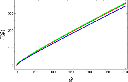
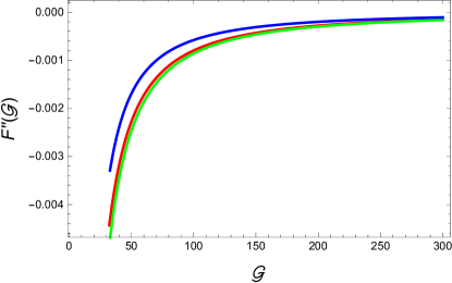
Figure 1: Evolution of holographic DE $F(\mathcal{G})$ model (left) and $F^{\prime\prime}(\mathcal{G})$ (right) versus $\mathcal{G}$ for $\lambda=1.5$ (red), $\lambda=2$ (green) and $\lambda=2.4$ (blue).

Figure 1 shows the graphical analysis of holographic DE $F(\mathcal{G})$ model in the left panel while the right plot demonstrates its stability with the parameters chosen as $d_{1}=5,~{}d_{2}=d_{3}=1$ and $\chi=-2.74$ throughout the analysis. We observe that the reconstructed model exhibits positively increasing behavior as $\mathcal{G}$ increases while it approaches zero as $\mathcal{G}\rightarrow 0$ for all the considered values of $\lambda$. It is important to mention here that stability of any $F(\mathcal{G})$ model depends on the regularity of generic function and its derivatives along with the condition $F^{\prime\prime}(\mathcal{G})<0$ for metric signatures $(+,-,-,-)$ while reverse inequality is required for the second choice of signatures for all $\mathcal{G}$ [52, 53]. Thus, the right plot shows that stability condition is satisfied for the reconstructed holographic DE $F(\mathcal{G})$ model.

3 Cosmological Analysis

In this section, we analyze the EoS and deceleration parameters as well as examine the cosmological planes such as $r-s$ and $\omega_{{}_{\mathcal{G}T}}-{\omega}^{\prime}_{{}_{\mathcal{G}T}}$ for the reconstructed holographic DE $f(\mathcal{G},T)$ model.

3.1 EoS Parameter

The EoS parameter for the obtained model using the correspondence scenario of energy densities is given by

$$\omega_{{}_{\mathcal{G}T}}=\frac{p_{{}_{\mathcal{G}T}}}{\rho_{\mathcal{G}T}}=\frac{p_{{}_{\mathcal{G}T}}}{\rho_{{}_{\Lambda}}}.$$ (25)

Carroll et al. [54] found that any phantom model with EoS parameter less than $-1$ should decay to $\omega=-1$ at late time in the context of general relativity using the scalar field Lagrangian density. Amirhashchi [55] observed that presence of bulk viscosity in the cosmic fluid can temporarily drive the fluid into the phantom region and ultimately EoS parameter of DE approaches to $-1$ as time passes. The presence of bulk viscosity in the background of anisotropic Bianchi I line element causes transition of EoS parameter of DE from quintessence to phantom which also decays to $-1$ at late time [56]. Amirhashchi [57] also analyzed the behavior of DE and found a possibility of DE EoS parameter to cross the phantom divide line for anisotropic Bianchi V spacetime.

We use scale factor in terms of red-shift parameter as $a=a_{\circ}(1+z)^{-1}$ throughout the graphical analysis. Figure 2 shows the cosmic evolutionary picture of EoS parameter against red-shift parameter $(z)$ using holographic DE model for $\lambda=2.4$. It is observed that EoS parameter represents the phantom regime at present $(z=0)$ and the corresponding value is $\omega_{{}_{\mathcal{G}T}}=-1.2$ consistent with Planck observational data [58] as well as in agreement with tilted flat and untitled non-flat XCDM model parameters constrained from Planck data [59]. It is also demonstrated from the graphical analysis that this parameter remains in the phantom regime and may not have a possibility to decay to $\omega_{{}_{\mathcal{G}T}}=-1$ at late time. Here, the phantom phase of the Universe is consistent with the observational data of holographic DE parameter $\tilde{c}$.

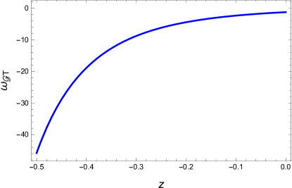
Figure 2: Evolution of EoS parameter versus $z$ for $\lambda=2.4$.

3.2 Deceleration Parameter

The deceleration parameter is defined as

$$q=-\frac{a\ddot{a}}{\dot{a}^{2}}=-1-\frac{\dot{H}}{H^{2}}.$$ (26)

Its positive value indicates the cosmic decelerated phase while negative value characterizes the epoch of accelerated expansion. Figure 3 shows the graphical cosmological evolution of deceleration parameter for the reconstructed model (24) against $z$. We observe that the value of this parameter is $-0.53$ at $z=0$ which is consistent with observational data of Planck [58] as well as favors the current constraints on isotropic and anisotropic DE models [60]. Thus, the holographic DE $f(\mathcal{G},T)$ model demonstrates the accelerating phase of the cosmic expansion.

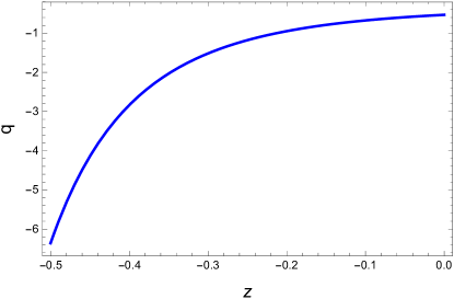
Figure 3: Evolution of deceleration parameter versus $z$ for $\lambda=2.4$.

3.3 $r-s$ Plane

Sahni et al. [61] introduced the cosmological diagnostic pair of dimensionless parameters known as state-finder diagnostic parameters to discriminate DE models such that one can determine which model is more suitable for a better explanation of the current cosmic status. These parameters are defined as

$$r=\frac{\dddot{a}}{aH^{3}}=2q^{2}+q-\frac{\dot{q}}{H},\quad s=\frac{r-1}{3\left(q-\frac{1}{2}\right)}.$$ (27)

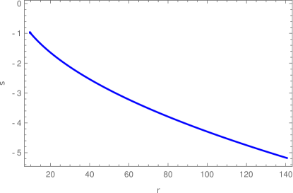
Figure 4: Plot of state-finder diagnostic parameters for $\lambda=2.4$.

The plane of these cosmological parameters (dubbed as $r-s$ plane) for $\Lambda$CDM model (CDM stands for cold dark matter) is fixed as $(r,s)=(1,0)$ while $(r,s)=(1,1)$ corresponds to CDM regime. The phantom as well as non-phantom DE epochs are illustrated by the regions ($r<1,s>0$) whereas trajectories for Chaplygin gas lie in the range ($r>1,s<0$). Figure 4 shows graphical interpretation of holographic DE $f(\mathcal{G},T)$ model in $r-s$ plane and observed that the evolutionary trajectory only correspond to the Chaplygin gas model.

3.4 $\omega_{{}_{\mathcal{G}T}}-{\omega}^{\prime}_{{}_{\mathcal{G}T}}$ Plane

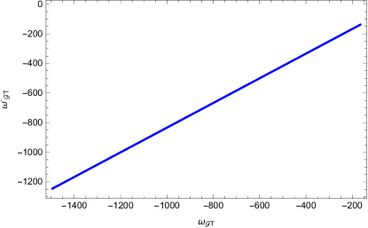
Figure 5: Plot of $\omega_{{}_{\mathcal{G}T}}-{\omega}^{\prime}_{{}_{\mathcal{G}T}}$ for $\lambda=2.4$.

Caldwell and Linder [62] presented $\omega_{{}_{\mathcal{G}T}}-{\omega}^{\prime}_{{}_{\mathcal{G}T}}$ (${\omega}^{\prime}_{{}_{\mathcal{G}T}}$ is the evolutionary form of ${\omega}_{{}_{\mathcal{G}T}}$ defined as ${\omega}^{\prime}_{{}_{\mathcal{G}T}}=d{\omega}_{{}_{\mathcal{G}T}}/d\ln a$) plane to investigate cosmic evolution of quintessence scalar field DE model and found that area occupied by the considered model in this plane can be categorized into freezing $(\omega<0,~{}\omega^{\prime}<0)$ and thawing ($\omega<0,~{}\omega^{\prime}>0$) regions. It is remarked that cosmic expansion is more accelerating in freezing region as compared to thawing. The graphical interpretation of $\omega_{{}_{\mathcal{G}T}}-{\omega}^{\prime}_{{}_{\mathcal{G}T}}$ is shown in Figure 5 which indicates the freezing region.

4 Final Remarks

In this paper, we have explored cosmological reconstruction of $f(\mathcal{G},T)$ gravity with a well-known holographic DE model using the power-law scale factor. The accelerated expansion of the Universe is considered as an outcome of integrated contribution from geometric and matter components. We have considered flat FRW Universe with pressureless matter contribution as cosmic fluid configuration and constructed the corresponding field equations for a particular form $f(\mathcal{G},T)=F(\mathcal{G})+\chi T$ ($\chi$ is an arbitrary constant). To reconstruct the holographic DE $F(\mathcal{G})$ model, we have applied the correspondence scheme by comparing the corresponding energy densities. The derived model possesses increasing behavior as well as satisfies the stability condition (Figure 1).

We have examined the evolutionary paradigm of reconstructed holographic $f(\mathcal{G},T)$ model through EoS and deceleration parameters as well as $r-s$ and $\omega_{{}_{\mathcal{G}T}}-{\omega}^{\prime}_{{}_{\mathcal{G}T}}$ cosmological planes. The results are summarized as follows.

• The trajectory of EoS parameter indicates the phantom phase of the Universe for the considered value of $\lambda$ at $z=0$ (Figure 2).

• The evolution of deceleration parameter against cosmic time gives accelerated phase of the Universe throughout the evolution (Figure 3).

• The state-finder diagnostic plane for the reconstructed model only corresponds to Chaplygin gas model (Figure 4).

• The trajectory in $\omega_{{}_{\mathcal{G}T}}-{\omega}^{\prime}_{{}_{\mathcal{G}T}}$ plane represents the freezing regime for the considered value of $\lambda$. Hence, $\omega_{{}_{\mathcal{G}T}}-{\omega}^{\prime}_{{}_{\mathcal{G}T}}$ plane shows consistency with the cosmic accelerated expansion (Figure 5).

Acknowledgement

We would like to thank the Higher Education Commission, Islamabad, Pakistan for its financial support through the Indigenous Ph.D. Fellowship for 5000 Scholars, Phase-II, Batch-III.

References

- [1] Nojiri, S. and Odintsov, S.D.: Phys. Rev. D 68(2003)123512.
- [2] Nojiri, S. and Odintsov, S.D.: Int. J. Geom. Methods Mod. Phys. 04(2007)115.
- [3] Nojiri, S. and Odintsov, S.D.: Phys. Rept. 505(2011)59.
- [4] Capozziello, S. and De Laurentis, M.: Phys. Rept. 509(2011)167.
- [5] Bamba, K. et al.: Astrophys. Space Sci. 342(2012)155.
- [6] Nojiri, S., Odintsov, S.D. and Oikonomou, V.K.: Phys. Rept. 692(2017)1.
- [7] Bhawal, B. and Kar, S.: Phys. Rev. D 46(1992)2464.
- [8] Deruelle, N. and Doleel, T.: Phys. Rev. D 62(2000)103502.
- [9] de Felice, A. and Tsujikawa, S.: Living Rev. Rel. 13(2010)3.
- [10] Nojiri, S., Odintsov, S.D. and Sasaki, M.: Phys. Rev. D 71(2005)123509.
- [11] Nojiri, S. and Odintsov, S.D.: Phys. Lett. B 631(2005)1.
- [12] Cognola, G. et al.: Phys. Rev. D 73(2006)084007.
- [13] de Felice, A. and Tsujikawa, S.: Phys. Rev. D 80(2009)063516.
- [14] Bamba, K. et al.: Eur. Phys. J. C 67(2010)295.
- [15] Odintsov, S.D., Oikonomou, V.K. and Saridakis, E.N.: Ann. Phys. 363(2015)141.
- [16] Harko, T. et al.: Phys. Rev. D 84(2011)024020.
- [17] Sharif, M. and Ikram, A.: Eur. Phys. J. C 76(2016)640.
- [18] Sharif, M. and Ikram, A.: Int. J. Mod. Phys. D 26(2017)1750084.
- [19] Sharif, M. and Ikram, A.: Eur. Phys. J. Plus 132(2017)526.
- [20] Shamir, M.F. and Ahmad, M.: Eur. Phys. J. C 77(2017)55.
- [21] Sharif, M. and Ikram, A.: Phys. Dark Universe 17(2017)1.
- [22] Li, M.: Phys. Lett. B 603(2004)1.
- [23] Susskind, L.: J. Math. Phys. 36(1995)6377; Hooft,G.’t.: arXiv:gr-qc/9310026.
- [24] Cohen, A.G., Kaplan, D.B. and Nelson, A.E.: Phys. Rev. Lett. 82(1999)4971.
- [25] Setare, M.R.: Int. J. Mod. Phys. D 17(2008)2219.
- [26] Setare, M.R. and Saridakis, E.N.: Phys. Lett. B 670(2008)1.
- [27] Karami, K. and Khaledian, M.S.: J. High Energy Phys. 03(2011)086.
- [28] Houndjo, M.J.S. and Piattella, O.F.: Int. J. Mod. Phys. D 21(2012)1250024.
- [29] Daouda, M.H., Rodrigues, M.E. and Houndjo, M.J.S.: Eur. Phys. J. C 72(2012)1893.
- [30] Jawad, A., Pasqua, A. and Chattopadhyay, S.: Eur. Phys. J. Plus 128(2013)156.
- [31] Sharif, M. and Zubair, M.: J. Phys. Soc. Jpn. 82(2013)064001.
- [32] Fayaz, V. et al.: Astrophys. Space Sci. 353(2014)301.
- [33] Sharif, M. and Zubair, M.: Astrophys. Space Sci 349(2014)529.
- [34] Zubair, M. and Abbas, G.: Astrophys. Space Sci. 357(2015)154.
- [35] Fayaz, V. et al.: Eur. Phys. J. Plus 131(2016)22.
- [36] Baffou, E.H., Houndjo, M.J.S. and Salako, I.G.: Int. J. Geom. Methods Mod. Phys. 14(2017)1750051.
- [37] Zubair, M. et al.: Symmetry 10(2018)463.
- [38] Tiwari, R.K., Beesham, A. and Shukla, B.: Int. J. Geom. Methods Mod. Phys. 15(2018)1850115.
- [39] Sharif, M. and Saba, S.: Mod. Phys. Lett. A 33(2018)1850182.
- [40] Landau, L.D. and Lifshitz, E.M.: The Classical Theory of Fields (Pergamon Press, 1971).
- [41] Li, M. et al.: J. Cosmol. Astropart. Phys. 09(2013)021.
- [42] Nojiri, S., Odintsov, S.D. and Tsujikawa, S.: Phys. Rev. D 71(2005)063004.
- [43] Oikonomou, V.K.: Phys. Rev. D 92(2015)124027.
- [44] Nojiri, S., Odintsov, S.D. and Tsujikawa, S.: Phys. Rev. D 71(2005)063004.
- [45] Nojiri, S., Odintsov, S.D. and Oikonomou, V.K.: Phys. Rev. D 91(2015)084059.
- [46] Nojiri, S. et al.: J. Cosmol. Astropart. Phys. 09(2015)044.
- [47] Odintsov, S.D. and Oikonomou, V.K.: Phys. Rev. D 92(2015)024016.
- [48] Oikonomou, V.K.: Int. J. Geom. Methods Mod. Phys. 13(2016)1650033.
- [49] Bahamonde, S. et al.: Ann. Phys. 373(2016)96.
- [50] Odintsov, S.D. and Oikonomou, V.K.: Phys. Rev. D 97(2018) 124042.
- [51] Odintsov, S.D. and Oikonomou, V.K.: Phys. Rev. D 98(2018)024013.
- [52] de Felice, A. and Tsujikawa, S.: Phys. Lett. B 675(2009)1.
- [53] Li, B., Barrow, J.D. and Mota, D.F.: Phys. Rev. D 76(2007)044027.
- [54] Carroll, S.M., Hoffman, M. and Trodden, M.: Phys. Rev. D 68(2003)023509.
- [55] Amirhashchi, H.: Astrophys. Space Sci. 345(2013)439.
- [56] Amirhashchi, H. and Pradhan, A.: Astrophys. Space Sci. 351(2014)59.
- [57] Amirhashchi, H.: Phys. Rev. D 96(2017)123507.
- [58] Ade, P.A.R. et al.: Astron. Astrophys.: 594(2016)A13.
- [59] Park, C.G. and Ratra, B.: arXiv:1803.05522.
- [60] Amirhashchi, H. and Amirhashchi, S.: Phys. Rev. D 99(2019)023516.
- [61] Sahni, V. et al.: J. Exp. Theor. Phys. Lett. 77(2003)201.
- [62] Caldwell, R.R. and Linder, E.V.: Phys. Rev. Lett. 95(2005)141301.