First-order Methods with Convergence Rates for Multi-agent Systems on Semidefinite Matrix Spaces

Abstract

The goal in this paper is to develop first-order methods equipped with convergence rates for multi-agent optimization problems on semidefinite matrix spaces. These problems include cooperative optimization problems and non-cooperative Nash games. Accordingly, first we consider a multi-agent system where the agents cooperatively minimize the summation of their local convex objectives, and second, we consider Cartesian stochastic variational inequality (CSVI) problems with monotone mappings for addressing stochastic Nash games on semidefinite matrix spaces. Despite the recent advancements in first-order methods addressing problems over vector spaces, there seems to be a major gap in the theory of the first-order methods for optimization problems and equilibriums on semidefinite matrix spaces. In particular, to the best of our knowledge, there exists no method with provable convergence rate for solving the two classes of problems under mild assumptions. Most existing methods either rely on strong assumptions, or require a two-loop framework where at each iteration, a projection problem, i.e., a semidefinite optimization problem, needs to be solved. Motivated by this gap, in the first part of the paper, we develop a mirror descent incremental subgradient method for minimizing a finite-sum function. We show that the iterates generated by the algorithm converge asymptotically to an optimal solution and derive a non-asymptotic convergence rate. In the second part, we consider semidefinite CSVI problems. We develop a stochastic mirror descent method that only requires monotonicity of the mapping. We show that the iterates generated by the algorithm converge to a solution of the CSVI almost surely. Using a suitably defined gap function, we derive a convergence rate statement. This work appears to be the first that provides a convergence speed guarantee for monotone CSVIs on semidefinite matrix spaces. Our numerical experiments performed on a multiple-input multiple-output multi-cell cellular wireless network support the convergence of the developed method.

1 Introduction

This paper addresses multi-agent problems over semidefinite matrix spaces including cooperative multi-agent problems and non-cooperative Nash games. First, we consider cooperative multi-agent problems. Decentralized optimization problems have a wide range of applications arising in data mining and machine learning (Nedić et al. (2017)), wireless sensor networks (Durham et al. (2012)), control (Ram et al. (2009)), and other areas in science and engineering (Xiao and Boyd (2006)) where decentralized processing of information is crucial for security purposes or for real-time decision making. In this paper, we consider the following multi-agent finite-sum optimization problem that involves a network of multiple agents who cooperatively optimize a global objective,

$$\underset{X\in\mathcal{B}}{\text{minimize}\ } \sum_{i=1}^{m}f_{i}(X)$$ (1)

where $\mathcal{B}\triangleq\{X\in\mathbb{S}_{n}:X\succeq 0$ and $\textnormal{tr}\!\left(X\right)=1\}$, and $f_{i}:\mathcal{B}\to\mathbb{R}$ is a convex function. Note that each agent $i$ is associated with the local objective $f_{i}(X)$ and all agents cooperatively minimize the network objective $\sum_{i=1}^{m}f_{i}(X)$. In decentralized optimization, the agents (players) need to communicate with their adjacent agents to spread the distributed information over the network and reach a consensus.

In the past two decades, there has been much interest in the development of models and distributed algorithms for multi-agent optimization problems. In particular, incremental gradient/subgradient methods and their accelerated aggregated variants (Nedić and Ozdaglar (2009), Lobel and Ozdaglar (2011), Shi et al. (2015), Gurbuzbalaban et al. (2017)) have been studied where a local gradient/subgradient is evaluated at each step of an iteration. Although each step is inexpensive, these methods usually require a large number of iterations to converge. Each iteration in decentralized optimization requires visiting all agents one by one which may cause a significant delay before a transfer of data begins. In this line of research, distributed proximal gradient methods (Bertsekas (2011, 2015)), and alternating direction method of multipliers (ADMM) (Chang et al. (2015), Makhdoumi and Ozdaglar (2017)) were developed and studied extensively as well. These methods have also been extended to applications where the network has a time-varying topology and/or there is a need to asynchronous implementations (Nedić (2011), Nedić and Olshevsky (2015)). Multi-agent mirror descent method for decentralized optimization was proposed by (Xi et al. (2014)) where a local Bregman divergence at each agent is employed, and an asymptotic convergence result is provided. More recently, Boţ and Böhm (2018) proposed an incremental mirror descent method with a stochastic sweeping of the component functions. While incremental gradient/subgradient methods and their accelerated aggregated variants are extensively studied in vector spaces, their performance and convergence analysis in matrix spaces have not been studied yet.

The sparse covariance estimation is a specific application of finite-sum problem which sets a certain number of coefficients in the inverse covariance to zero to improve the stability of covariance matrix estimation. Lu (2010) developed two first-order methods including the adaptive spectral projected gradient and the adaptive Nesterov’s smooth methods to solve the large scale covariance estimation problem. Hsieh et al. (2013) proposed a block coordinate descent (BCD) method with a superlinear convergence rate. In conic programming, first-order methods are equipped with duality or penalty strategies (Lan et al. (2011), Necoara et al. (2017)) to tackle complicated constraints. A major limitation to the aforementioned methods in addressing Problem (1) is that either they require a projection step that is computationally costly in the semidefinite space, or they employ Lagrangian relaxation techniques slowing down the convergence speed of the underlying first-order method. Accordingly, in the first part of the paper, we address this gap by developing a matrix mirror descent incremental subgradient (M-MDIS) method to solve finite-sum Problem (1) where we choose the distance generating function to be defined as the quantum entropy following Tsuda et al. (2005). M-MDIS is a first-order method in the sense that it only requires a gradient-type of update at each iteration. This method is a single-loop algorithm meaning that it provides a closed-form solution for the projected point and hence it does not need to solve a projection problem at each iteration. We prove that M-MDIS method converges to the optimal solution of (1) asymptotically and derive a non-asymptotic convergence rate of $\mathcal{O}(1/\sqrt{t})$.

In the second part of the paper, we consider non-cooperative multi-agent systems. In addressing such problems, variational inequalities (VIs) were first introduced in the 1960s. VIs have a wide range of applications arising in engineering, finance, physics and economics (cf. Facchinei and Pang (2007)). They can be used for formulating various equilibrium problems and analyzing them from the viewpoint of existence and uniqueness of solutions and stability. Particularly, in mathematical programming, VIs address problems such as optimization problems, complementarity problems and systems of nonlinear equations, to name a few (Scutari et al. (2010)). Given a set ${\mathcal{X}}$ and a mapping $F:\mathbf{\mathcal{X}}\to\mathbb{R}^{n\times n}$, a VI problem denoted by VI$(\mathbf{\mathcal{X}},F)$ seeks a matrix $X^{*}\in\mathbf{\mathcal{X}}$ such that $\textnormal{tr}\!\left((X-X^{*})^{T}F(X^{*})\right)\geq 0,\quad\text{for all}~{}X\in{\mathcal{X}}.$ In addressing non-cooperative Nash games, we consider Cartesian stochastic variational inequality (CSVI) problems where the set $\mathcal{X}$ is a Cartesian product of some component sets $\mathcal{X}_{i}$, i.e.,

$${\mathcal{X}}\triangleq\{X\in\mathbb{S}_{n}|X=\text{diag}(X_{1},\ldots,X_{N}),~{}X_{i}\in\mathcal{X}_{i}\},$$

$$\text{where}~{}\mathcal{X}_{i}\triangleq\{X_{i}\in\mathbb{S}^{+}_{n_{i}}|\textnormal{tr}\!\left(X_{i}\right)=1\}\quad\text{for all}\quad i=1,\ldots,N.$$ (2)

Hence, we seek a matrix $X^{*}=\text{diag}(X^{*}_{1},\ldots,X^{*}_{N})$ that solves the following inequality for all $i=1,\ldots,N$:

$$\textnormal{tr}\!\left((X_{i}-X_{i}^{*})^{T}F_{i}(X^{*})\right)\geq 0,\quad\text{for all}~{}X_{i}\in{\mathcal{X}_{i}}.$$ (3)

In particular, we study VI($\mathbf{\mathcal{X}},F$) where $F_{i}(X)=\mathbb{E}[\Phi_{i}(X,\xi_{i}(w))]$, i.e., the mapping $F_{i}$ is the expected value of a stochastic mapping $\Phi_{i}:{\mathcal{X}}\times\mathbb{R}^{d_{i}}\to\mathbb{S}_{n}$ where the vector $\xi_{i}:\Omega\to\mathbb{R}^{d_{i}}$ is a random vector associated with a probability space represented by $(\Omega,\mathcal{F},\mathbb{P})$. Here, $\Omega$ denotes the sample space, $\mathcal{F}$ denotes a $\sigma$-algebra on $\Omega$, and $\mathbb{P}$ is the associated probability measure. Therefore, $X^{*}\in\mathbf{\mathcal{X}}$ solves VI($\mathbf{\mathcal{X}},F$) if for all $i=1,\ldots,N$,

$$\textnormal{tr}\!\left((X_{i}-X_{i}^{*})^{T}\mathbb{E}[\Phi_{i}(X^{*},\xi(w))]\right)\geq 0,~{}\text{for all}~{}X_{i}\in{\mathcal{X}_{i}}.$$ (4)

Throughout, we assume that $\mathbb{E}[\Phi_{i}(X^{*},\xi_{i}(w))]$ is well-defined (i.e., the expectation is finite). There are several challenges in solving CSVIs on semidefinite matrix spaces including presence of uncertainty, the semidefinite solution space and the Cartesian product structure. In what follows, we review some of the methods that address these challenges, and explain their limitations.

Stochastic Approximation (SA) schemes (Robbins and Monro (1951)) and their prox generalization (Nemirovski et al. (2009), Majlesinasab et al. (2019b)) shown to be very successful in solving optimization and VI problems (Jiang and Xu (2008)) with uncertainties. Averaging techniques first introduced by Polyak and Juditsky (1992) proved successful in increasing the robustness of the SA method. Applying SA schemes to solve semidefinite optimization problems result in a two-loop framework and require projection onto a semidefinite cone at each iteration which increases the computational complexity.

Solving optimization problems with positive semidefinite variables is more challenging than solving problems in vector spaces because of the structure of problem constraints. Matrix exponential learning (MEL) which has strong ties to mirror descent methods is an optimization algorithm applied to positive semidefinite nonlinear problems. The distance generating function applied in MEL is the quantum entropy. Mertikopoulos et al. (2012) proposed an MEL based approach to solve the power allocation problem in multiple-input multiple-output (MIMO) multiple access channels. The convergence of MEL and its robustness w.r.t. uncertainties are investigated by Mertikopoulos and Moustakas (2016). Although in the above studies, the problem can be formulated as an optimization problem, some practical cases such as multi-user MIMO maximization problem discussed in Section 2 cannot be treated as an optimization problem. Hence, Mertikopoulos et al. (2017) proposed an MEL based algorithm to solve $N$-player games under uncertain feedback and proved that it converges to a stable Nash equilibrium assuming that the mapping is strongly stable. However, in most applications including the game (8) this assumption is not met.

In the VI regime, the focus has been more on addressing stochastic VIs (SVIs) on vector spaces. In particular, CSVIs on matrix spaces which have applications in wireless networks and image retrieval (cf. Section 2) have not been studied yet. In addressing these limitations, we consider CSVIs on matrix spaces where the mapping is merely monotone. We develop an averaging matrix stochastic mirror descent (A-M-SMD) method to solve CSVI (4). A-M-SMD is a first-order single-loop algorithm. To drive rate statements and to improve its robustness w.r.t. uncertainties, we employ averaging techniques. In the second part of the paper, we improve the MEL method of Mertikopoulos et al. (2017) in the sense that we require an applicable assumption on the mapping since strong stability of the mapping either does not hold in applications, or it is hard to be verified. The originality of this work lies in the convergence and rate analysis under the monotonicity assumption. We establish convergence to a weak solution of the CSVI by introducing an auxiliary sequence. Then, we derive a convergence rate of $\mathcal{O}(1/\sqrt{t})$ in terms of the expected value of a suitably defined gap function. Our work is amongst the first ones that provide a convergence rate for CSVI on semidefinite matrix spaces. In Table 1, the distinctions between the existing methods and our work are summarized. We apply the A-M-SMD method on a throughput maximization problem in wireless multi-user MIMO networks. Our results show that the A-M-SMD scheme has a robust performance w.r.t. uncertainty and problem parameters and outperforms both non-averaging M-SMD and MEL methods.

Table 1: Comparison of first-order schemes

Reference	Problem	Assumptions	Space	Scheme	1-loop	Rate
Lan et al. (2011)	Opt	C,S/NS	Matrix	Primal-dual Nesterov’s methods	✗	${\cal O}\left({1}/{t}\right)$
Hsieh et al. (2013)	Opt	NS,C	Matrix	BCD	✗	superlinear
Bertsekas (2015)	finite-sum	C,S	Vector	Incremental Aggregated Proximal	✗	Linear
Gurbuzbalaban et al. (2017)	finite-sum	C,S	Vector	Incremental Aggregated Gradient	✗	Linear
Boţ and Böhm (2018)	finite-sum	C,NS	Vector	Incremental SMD	✗	${\cal O}\left({1}/{\sqrt{t}}\right)$
Our work	finite-sum	MM, NS	Matrix	M-MDIS	✓	${\cal O}\left({1}/{\sqrt{t}}\right)$
Jiang and Xu (2008)	SVI	SM,S	Vector	SA	✗	$-$
Juditsky et al. (2011)	SVI	PM,S/NS	Vector	Extragradient SMP	✗	${\cal O}\left({1}/{t}\right)$
Mertikopoulos et al. (2012)	SOpt	C,S	Matrix	Exponential Learning	✓	$e^{-\alpha t}{\color[rgb]{0,0,0}(\alpha>0)}$
Koshal et al. (2013)	SVI	MM,S	Vector	Regularized Iterative SA	✗	$-$
Yousefian et al. (2017)	SVI	MM,NS	Vector	Regularized Smooth SA	✗	${\cal O}\left({1}/{\sqrt{t}}\right)$
Mertikopoulos et al. (2017)	SVI	SL,S	Matrix	Exponential Learning	✓	${\cal O}\left({1}/{\lambda t}\right)$
Yousefian et al. (2018)	CSVI	PM,S	Vector	Averaging B-SMP	✗	${\cal O}\left({1}/{t}\right)$
Our work	SVI	MM, NS	Matrix	A-M-SMD	✓	${\cal O}\left({1}/{\sqrt{t}}\right)$

SM: strongly monotone mapping, MM: merely monotone mapping,  PM: psedue-monotone mapping, C: convex,

SL: strongly stable mapping,  S: smooth function NS: nonsmooth function,

Opt: optimzation problem,  $\lambda$: strong stability parameter

Remark 1.

It should be noted that the accelerated variants of first-order methods such as SVRG (Johnson and Zhang (2013)), SAGA (Defazio et al. (2014)) and IAG (Gurbuzbalaban et al. (2017)) provide improved rate guarantees for optimization and VI problems (Chen et al. (2017)) on vector spaces. Developing this type of methods for solving finite-sum and CSVI problems on matrix spaces and providing their convergence analysis can be a direction for future research.

The paper is organized as follows. Section 2 presents the motivation and source problems. In Section 3, the von Neumann divergence and its main properties are discussed and some results that are applied in the analysis of the paper are established. In Section 4, we address the finite-sum Problem (1), outline a matrix mirror descent incremental subgradient method and provide its convergence analysis. In Section 5, we present an averaging matrix stochastic mirror descent algorithm for solving CSVI (4) and analyze its convergence. We report the numerical experiments in Section 6 and conclude in Section 7.

Notation: Throughout, $\mathbb{S}_{n}$ denotes the set of all $n\times n$ symmetric matrices and $\mathbb{S}_{n}^{+}$ the cone of all positive semidefinite matrices. The mapping $F:\mathcal{X}\to\mathbb{R}^{n\times n}$ is called monotone if for any $X,Y\in\mathcal{X}$, we have $\textnormal{tr}\!\left((X-Y)(F(X)-F(Y))\right)\geq 0$. The set of solutions to VI($\mathbf{\mathcal{X}},F$) is denoted by $\text{SOL}({\mathcal{X}},\mathit{F})$. We define the set $\mathscr{X}\triangleq\{X\in\mathbb{S}_{n}^{+}|\textnormal{tr}\!\left(X\right)\leq 1\}$. We let $[A]_{uv}$ denote the components of matrix $A$. $\mathbb{C}$ is the set of complex numbers. The spectral norm of a matrix $A$ being the largest singular value of $A$ is denoted by the norm $\|A\|_{2}$. The trace norm of a matrix $A$ being the sum of singular values of the matrix is denoted by $\textnormal{tr}\!\left(A\right)$. Note that spectral and trace norms are dual to each other (Fazel et al. (2001)). We let $\mathbf{A}^{\dagger}$ denote the conjugate transpose of matrix $\mathbf{A}$. A square matrix $A$ that is equal to its conjugate transpose is called Hermitian. We let $\mathbb{H}_{n}$ denote the set of all $n\times n$ Hermitian matrices.

2 Motivation and Source Problems

Our research is motivated by the following problems:

• Example on cooperative multi-agent problems: distributed sparse estimation of covariance inverse

  Given a set of samples $\{z_{i}^{j}\}_{j=1}^{n_{i}}$ associated with agent $i$, where $z_{i}^{j}\sim\mathcal{N}(\mu,\Sigma)$, $n_{i}$ is the sample size of the $i$th agent, $\mu\in\mathbb{R}^{d}$ and $\Sigma\in\mathbb{R}^{d\times d}$ are the mean and covariance matrix of a multivariate Gaussian distribution, respectively. To estimate $\mu$ and $\Sigma$, consider the maximum likelihood estimators (MLE) given by

  $$\hat{\mu},\hat{\Sigma}=\underset{\mu,\Sigma}{\text{argmax}}\prod_{i=1}^{m}\prod_{j=1}^{n_{i}}\frac{1}{\sqrt{(2\pi)^{n_{i}}\text{det}(\Sigma)}}\text{exp}\left(-\frac{1}{2}(z_{i}^{j}-\mu)^{T}\Sigma^{-1}(z_{i}^{j}-\mu)\right).$$

  This equation can then be cast as a distributed inverse covariance estimation problem

  $$\underset{\Sigma^{-1}\succ 0}{\text{min}}-\sum_{i=1}^{m}\text{log}\left(\text{det}\Sigma^{-1}\right)+\sum_{i=1}^{m}\textnormal{tr}\!\left(S_{i}\Sigma^{-1}\right),$$

  where $S_{i}\triangleq\frac{1}{n_{i}}\sum_{j=1}^{n_{i}}-\frac{1}{2}(z_{i}^{j}-\hat{\mu}_{i})^{T}(z_{i}^{j}-\hat{\mu}_{i})$ with $\hat{\mu}_{i}\triangleq\frac{1}{n_{i}}\sum_{j=1}^{n_{i}}z_{i}^{j}$. To induce sparsity, consider adding a lasso penalty of the form $\lambda\|P\ast\Sigma^{-1}\|_{1}$ to the likelihood as follows

  $$\underset{\Sigma^{-1}\succ 0}{\text{min}}-\sum_{i=1}^{m}\text{log}\left(\text{det}\Sigma^{-1}\right)+\sum_{i=1}^{m}\textnormal{tr}\!\left(S_{i}\Sigma^{-1}\right)+\lambda\|P\ast\Sigma^{-1}\|_{1},$$ (5)

  where $P$ is a suitable matrix with nonnegative elements, $\lambda>0$ is the regularization parameter, and $\ast$ denotes element-wise multiplication. For a matrix $A$, we define $\|A\|_{1}=\sum_{i,j}|[A]_{ij}|$. Two common choices for $P$ would be the matrix of all ones or this matrix with zeros on the diagonal to avoid shrinking diagonal elements of $\Sigma$ (Bien and Tibshirani (2011)). Problem (5) can be viewed as an instance of Problem (1), where we define $f_{i}(\Sigma^{-1})=-\text{log}\left(\text{det}\Sigma^{-1}\right)+\textnormal{tr}\!\left(S_{i}\Sigma^{-1}\right)+\frac{\lambda}{m}\|P\ast\Sigma^{-1}\|_{1}.$

  Remark 2.

  We propose M-MDIS algorithm to solve Problem (1). It should be noted that the constraint $\textnormal{tr}\!\left(X\right)=1$ makes the analysis more complicated. Our Analysis can be easily extended to the cases similar to the sparse covariance estimation problem where this constraint does not exist.

• Stochastic non-cooperative Nash games: In a non-cooperative game, $N$ players (users) with conflicting interests compete to minimize their own payoff function. Suppose each player controls a positive semidefinite matrix variable $X_{i}\in\mathcal{X}_{i}$ where $\mathcal{X}_{i}$ denotes the set of all possible actions of player $i$. We let $X_{-i}\triangleq(X_{1},...,X_{i-1},X_{i+1},...,X_{N})$ denote the possible actions of other players and $f_{i}(X_{i},X_{-i})$ denote the payoff function of player $i$. Therefore, the following Nash game needs to be solved

  $$\underset{X_{i}\in\mathcal{X}_{i}}{\text{minimize}}\quad f_{i}(X_{i},X_{-i}),\quad\text{for all}~{}i=1,\cdots,N,$$ (6)

  which includes $N$ semidefinite optimization problems. A solution $X^{*}=\left(X^{*}_{1},\ldots,X^{*}_{N}\right)$ to this game, called a Nash equilibrium, is a feasible action profile such that $f_{i}(X_{i}^{*},X_{-i}^{*})\leq f_{i}(X_{i},X^{*}_{-i})$, for all $X_{i}\in\mathcal{X}_{i}=\{X_{i}\in\mathbb{S}^{+}_{n_{i}}|~{}\textnormal{tr}\!\left(X_{i}\right)=1\}$, $i=1,\ldots,N$. Later, in Lemma 4, we prove that the optimality conditions of Nash game (6) can be formulated as a VI$(\mathbf{\mathcal{X}},F)$ where $\mathcal{X}\triangleq\{X|X=\text{diag}(X_{1},\cdots,X_{N}),\>X_{i}\in\mathcal{X}_{i},~{}\text{for all}~{}i=1,\ldots,N\}$ and $F(X)\triangleq\text{diag}(\nabla_{X_{1}}f_{1}(X),\cdots,\nabla_{X_{N}}f_{N}(X))$. Next, we discuss one of the applications of Problem (6) in wireless communication network.

  Wireless Communication Networks: A wireless network is composed of transmitters and receivers that generate and detect radio signals, respectively. An antenna enables a transmitter to send signals into the space, and enables a receiver to pick up signals from the space. In a multiple-input multiple-output (MIMO) wireless transmission system, multiple antennas are applied in transmitters and receivers in order to improve the performance. In some MIMO systems such as MIMO broadcast channels and MIMO multiple access channels, there are multiple users with mutual interferes. In recent years, MIMO systems under uncertainty have been studied where the state channel information is subject to noise, delays and other imperfections (Mertikopoulos et al. (2017)). Here, our problem of interest is the throughput maximization in multi-user MIMO networks under feedback errors. In this network, $N$ MIMO links (users) compete where each link $i$ represents a pair of transmitter-receiver with $m_{i}$ antennas at the transmitter and $n_{i}$ antennas at the receiver. Let $\mathbf{x}_{i}\in\mathbb{C}^{n_{i}}$ and $\mathbf{y}_{i}\in\mathbb{C}^{m_{i}}$ denote the signal transmitted from and received by the $i$th link, respectively. The signal model can be described by $\mathbf{y}_{i}={H}_{ii}\mathbf{x}_{i}+\sum\nolimits_{j\neq i}{H}_{ji}\mathbf{x}_{j}+\mathbf{\epsilon}_{i}$, where ${H}_{ii}\in\mathbb{C}^{m_{i}\times n_{i}}$ is the direct-channel matrix of link $i$, ${H}_{ji}\in\mathbb{C}^{m_{i}\times n_{j}}$ is the cross-channel matrix between transmitter $j$ and receiver $i$, and $\mathbf{\epsilon}_{i}\in\mathbb{C}^{m_{i}}$ is a zero-mean circularly symmetric complex Gaussian noise vector with the covariance matrix $\mathbf{I}_{m_{i}}$ (Mertikopoulos and Moustakas (2016)). Each transmitter $i$ tries to improve its performance by transmitting at its maximum power level. Hence, the action for each player is the transmit power. However, doing so results in a conflict in the system since the overall interference increases and affects the capability of all involved transmitters. Here, we consider the interference generated by other users as an additive noise. Therefore, $\sum_{j\neq i}{H}_{ji}\mathbf{x}_{j}$ represents the multi-user interference (MUI) received by the $i$th player and generated by other users. Assuming the random vector $\mathbf{x}_{i}$ follows a complex Guassian distribution, transmitter $i$ controls its input signal covariance matrix $X_{i}\triangleq\mathbb{E}[\mathbf{x}_{i}\mathbf{x}_{i}^{\dagger}]$ subject to two constraints: first the signal covariance matrix is positive semidefinite and second each transmitter’s maximum transmit power is set to a positive scalar $p$. Under these assumptions, each user’s transmission throughput for a given set of users’ covariance matrices $X_{1},\ldots,X_{N}$ is given by

  $$R_{i}(X_{i},X_{-i}) =\log\det\left(\mathbf{I}_{m_{i}}+\sum\nolimits_{j=1}^{N}H_{ji}X_{j}H_{ji}^{\dagger}\right)-\log\det(W_{-i}),$$ (7)

  where $W_{-i}=\mathbf{I}_{m_{i}}+\sum_{j\neq i}H_{ji}X_{j}H_{ji}^{\dagger}$ is the MUI-plus-noise covariance matrix at receiver $i$ (Telatar (1999)). Let $\mathcal{X}_{i}=\{X_{i}\in\mathbb{C}^{n_{i}\times n_{i}}:X_{i}\succeq 0$, $\textnormal{tr}\!\left(X_{i}\right)=p\}$. The goal is to solve

  $$\underset{X_{i}\in\mathcal{X}_{i}}{\text{maximize}}\quad R_{i}(X_{i},X_{-i}),\quad\text{for all}~{}i=1,\ldots,N.$$ (8)

In section 6, we present the implementation of our scheme in addressing Problem (8).

3 Preliminaries

Suppose $\omega:\text{dom}(\omega)\to\mathbb{R}$ is a strictly convex and differentiable function, where $\text{dom}(\omega)\subseteq\mathbb{R}^{n\times n}$, and let $X,Y\in\text{dom}(\omega)$. Then, Bregman divergence between $X$ and $Y$ is defined as $D(X,Y):=\omega(X)-\omega(Y)-\textnormal{tr}\!\left((X-Y)\nabla\omega(Y)^{T}\right).$ In what follows, our choice of $\omega$ is the quantum entropy (Vedral (2002)),

$$\omega(X)\triangleq\left\{\begin{array}[]{rl}\textnormal{tr}\!\left(X\log X-X\right)&~{}\text{if }\quad X\in\mathcal{B},\\ +\infty&\quad\text{otherwise},\end{array}\right.$$ (9)

where $\mathcal{B}\triangleq\{X\in\mathbb{S}_{n}:X\succeq 0$ and $\textnormal{tr}\!\left(X\right)=1\}$. The Bregman divergence corresponding to the quantum entropy is called von Neumann divergence and is given by

$$D(X,Y)=\textnormal{tr}\!\left(X\log X-X\log Y\right)$$ (10)

(Tsuda et al. (2005)). In our analysis, we use the following property of $\omega$.

Lemma 1.

(Yu (2013)) Let $\mathscr{X}\triangleq\{X\in\mathbb{S}_{n}^{+}|\textnormal{tr}\!\left(X\right)\leq 1\}$. The quantum entropy $\omega:\mathscr{X}\to\mathbb{R}$ is strongly convex with modulus 1 under the trace norm.

Since $\mathcal{B}\subset\mathbf{\mathscr{X}}$, the quantum entropy $\omega:{\mathcal{B}}\to\mathbb{R}$ is also strongly convex with modulus 1 under the trace norm. Next, we derive the conjugate of the quantum entropy and its gradient.

Lemma 2 (Conjugate of von Neumann entropy).

Let $Y\in\mathbb{S}_{n}$ and $\omega(X)$ be defined as (9). Then, we have

$$\omega^{*}(Y)=\log(\textnormal{tr}\!\left(\exp(Y+I_{n})\right)),$$ (11)

$$\nabla\omega^{*}(Y)=\frac{\exp(Y+I_{n})}{\textnormal{tr}\!\left(\exp(Y+I_{n})\right)}.$$ (12)

Proof.

Note that $\omega$ is a lower semi-continuous convex function on the linear space of all symmetric matrices. The conjugate of function $\omega$ is defined as

$$\omega^{*}({Y})=\sup\{\textnormal{tr}\!\left(DY\right)-\omega(D):~{}D\in\mathcal{B}\}=\sup\{\textnormal{tr}\!\left(DY\right)-\textnormal{tr}\!\left(D\log D-D\right):D\in\mathcal{B}\}$$

$$=-\inf\{-\underbrace{\textnormal{tr}\!\left(D(Y+I_{n})\right)+\textnormal{tr}\!\left(D\log D\right)}_{\text{Term 1}},~{}D\in\mathcal{B}\}.$$ (13)

The minimizer of the above problem is $\displaystyle D=\frac{\exp(Y+I_{n})}{\textnormal{tr}\!\left(\exp(Y+I_{n})\right)}$ which is called the Gibbs state (see Hiai and Petz (2014), Example 3.29). By plugging it into Term 1, we have (11). The relation (12) follows by standard matrix analysis and the fact that $\nabla_{Y}\textnormal{tr}\!\left(\exp(Y)\right)=\exp(Y)$ (Athans and Schweppe (1965)). We observe that $\nabla\omega^{*}(Y)$ is a positive semidefinite matrix with a trace equal to one, implying that $\nabla\omega^{*}(Y)\in\mathcal{B}$. ∎

Next, we show that the optimality conditions of a matrix constrained optimization problem can be formulated as a VI. The proof can be found in the Appendix.

Lemma 3.

Let $\mathcal{B}\subseteq\mathbb{R}^{n\times n}$ be a nonempty closed convex set, and let $f:\mathbb{R}^{n\times n}\to\mathbb{R}$ be a differentiable convex function. Consider the optimization problem

$$\underset{\widetilde{X}\in\mathcal{B}}{\text{minimize}}\quad f(\widetilde{X}).$$ (14)

A matrix $\widetilde{X}^{*}$ is optimal to Problem (14) iff $\widetilde{X}^{*}\in\mathcal{B}$ and $\textnormal{tr}\!\left((Z-\widetilde{X}^{*})^{T}\nabla f(\widetilde{X}^{*})\right)\geq 0$, for all $Z\in\mathcal{B}$.

The next Lemma shows a set of sufficient conditions under which a Nash equilibrium can be obtained by solving a VI.

Lemma 4 (Nash equilibrium).

Let $\mathcal{X}_{i}\subseteq\mathbb{S}_{n_{i}}$ be a nonempty closed convex set and $f_{i}(X_{i},X_{-i})$ be a differentiable convex function in $X_{i}$ for all $i=1,\cdots,N$, where $X_{i}\in\mathcal{X}_{i}$ and $X_{-i}\in\prod_{j\neq i}{\mathcal{X}_{j}}$. Then, $X^{*}\triangleq\text{diag}(X_{1}^{*},\cdots,X_{N}^{*})$ is a Nash equilibrium (NE) to game (6) if and only if $X^{*}$ solves VI($\mathbf{\mathcal{X}},F$), where

$$F(X)\triangleq\text{diag}(\nabla_{X_{1}}f_{1}(X),\cdots,\nabla_{X_{N}}f_{N}(X)),$$ (15)

$$\mathcal{X}\triangleq\{X|X=\text{diag}(X_{1},\cdots,X_{N}),\>X_{i}\in\mathcal{X}_{i},~{}\text{for all}~{}i\}.$$ (16)

Proof.

First, suppose $X^{*}$ is an NE to game (6). We want to prove that $X^{*}$ solves VI($\mathbf{\mathcal{X}},F$), i.e, $\textnormal{tr}\!\left((Z-X^{*})^{T}F(X^{*})\right)\geq 0$, for all $Z\in\mathcal{X}$. By optimality conditions of optimization problem $\underset{X_{i}\in\mathcal{X}_{i}}{min}\ f_{i}(X_{i},X_{-i})$ and from Lemma 3, we know $X^{*}$ is an NE if and only if $\textnormal{tr}\!\left((Z_{i}-X_{i}^{*})^{T}\nabla_{X_{i}}f_{i}(X^{*})\right)\geq 0$ for all $Z_{i}\in\mathcal{X}_{i}$ and all $i=1,\ldots,N$. Then, we obtain for all $i=1,\cdots,N$

$$\textnormal{tr}\!\left((Z_{i}-X_{i}^{*})^{T}\nabla_{X_{i}}f_{i}(X^{*})\right)=\sum_{u}\sum_{v}[Z_{i}-X_{i}^{*}]_{uv}[\nabla_{X_{i}}f_{i}(X^{*})]_{uv}\geq 0.$$ (17)

Invoking the definition of mapping $F$ given by (15) and from (17), we have $\textnormal{tr}\!\left((Z-X^{*})^{T}F(X^{*})\right)=\sum_{i,u,v}[Z_{i}-X_{i}^{*}]_{uv}[\nabla_{X_{i}}f_{i}(X^{*})]_{uv}\geq 0.$ From the definition of VI($\mathbf{\mathcal{X}},F$) and relation (3), we conclude that $X^{*}\in\text{SOL}({\mathcal{X}},\mathit{F})$. Conversely, suppose $X^{*}\in\text{SOL}({\mathcal{X}},\mathit{F})$. Then, $\textnormal{tr}\!\left((Z-X^{*})^{T}F(X^{*})\right)\geq 0,\text{for all}\>Z\in\mathcal{X}$. Consider a fixed $i\in\{1,\ldots,N\}$ and a matrix $\bar{Z}\in\mathcal{X}$ given by (16) such that the only difference between $X^{\ast}$ and $\bar{Z}$ is in $i$-th block, i.e.

$$\bar{Z}=\text{diag}\left(\left[X_{1}^{*}\right],\ldots,\left[X_{i-1}^{*}\right],\left[Z_{i}\right],\left[X_{i+1}^{*}\right],\ldots,\left[X_{N}^{*}\right]\right),$$

where $Z_{i}$ is an arbitrary matrix in $\mathcal{X}_{i}$. Then, we have

$$\bar{Z}-X^{*}=\text{diag}\left(\mathbf{0}_{n_{1}\times n_{1}},\ldots,\left[Z_{i}-X_{i}^{*}\right],\ldots,\mathbf{0}_{n_{N}\times n_{N}}\right).$$ (18)

Therefore, substituting $\bar{Z}-X^{*}$ by term (18), we obtain

$$\textnormal{tr}\!\left((\bar{Z}-X^{*})^{T}F(X^{*})\right)=\sum_{u}\sum_{v}[(Z_{i}-X_{i}^{*})]_{uv}[\nabla_{X_{i}}f_{i}(X^{*})]_{uv}=\textnormal{tr}\!\left((Z_{i}-X_{i}^{*})^{T}\nabla_{X_{i}}f_{i}(X^{*})\right)\geq 0.$$

Since $i$ was chosen arbitrarily, $\textnormal{tr}\!\left((Z_{i}-X_{i}^{*})^{T}\nabla_{X_{i}}f_{i}(X^{*})\right)\geq 0$ for any $i=1,...,N$. Hence, by applying Lemma 3 we conclude that $X^{*}$ is a Nash equilibrium to game (6). ∎

4 Cooperative multi-agent problems

Consider the multi-agent optimization Problem (1) on semidefinite matrix spaces. In this section, we present the mirror descent incremental subgradient method for solving (1). Algorithm 1 presents the outline of the M-MDIS method. The method maintains two matrices for each agent $i$: primal $U_{i}$ and dual $Y_{i}$. The connection between the two matrices is via a function $U_{i}=\nabla\omega^{*}(Y_{i})$ which projects $Y_{i}$ onto the set $\mathcal{B}$ defined by (1). At each iteration $t$ and for any agent $i$, first, the subgradient of $f_{i}$ is calculated at $U_{i-1,t}$, denoted by $\tilde{\nabla}f_{i}(U_{i-1,t})$. Next, we update the dual matrix by moving along the subgradient. Here $\eta_{t}$ is a non-increasing step-size sequence. Then, $Y_{i,t}$ will be projected onto the set $\mathcal{B}$ using the closed-form solution (20). It should be noted that the update rule (20) is obtained by applying Lemma 2. Finally, the primal and dual matrices of agent $m$, i.e. $U_{m,t}$ and $Y_{m,t}$ are the input to the next iteration.

Algorithm 1 Matrix Mirror Descent Incremental Subgradient (M-MDIS)

  1: initialization: pick $X_{0}\in\mathcal{B}$, and $Y_{m,-1}\in\mathbb{S}_{n}$ arbitrarily.

  2: General step: for any $t=0,1,2,\cdots$ do the following:

• $U_{0,t}:=X_{t}$ and $Y_{0,t}:=Y_{m,t-1}$

• For i=1,…,$m$ do the following:

  $$Y_{i,t}:=Y_{i-1,t}-\eta_{t}\tilde{\nabla}f_{i}(U_{i-1,t})$$ (19)

  $$U_{i,t}:=\displaystyle\frac{\exp(Y_{i,t}+\mathbf{I}_{n})}{\textnormal{tr}\!\left(\exp(Y_{i,t}+\mathbf{I}_{n})\right)}$$ (20)

• $X_{t+1}:=U_{m,t}$.

Next, we state the main assumption and discuss its rationality.

Assumption 1.

Let the set $\mathcal{B}\triangleq\{X\in\mathbb{S}_{n}:X\succeq 0$ and $\textnormal{tr}\!\left(X\right)=1\}$. The functions $f_{i}$’s are proper and convex on $\mathcal{B}$.

Remark 3 (Boundedness of subgradients).

Under Assumption 1, the union $\underset{X\in\mathcal{B}}{\cup}\partial f_{i}(X)$ is nonempty and bounded (Beck (2017), Theorem 3.16). Therefore, there exists a constant $L_{f_{i}}$ for which $\|\tilde{\nabla}f_{i}(X)\|_{2}\leq L_{f_{i}}$ for all $\tilde{\nabla}f_{i}(X)\in\partial f_{i}(X)$, $X\in\mathcal{B}$ and for all $i=1,\ldots,m$.

We use the following relation in the convergence analysis,

$$Y_{i,t}\triangleq\tilde{\nabla}\omega(U_{i,t})\in\partial\omega(U_{i,t})\Leftrightarrow U_{i,t}\in\partial\omega^{\star}(Y_{i,t}).$$ (21)

It should be noted that the above relation holds because $\omega$ is a closed and convex function (Rockafellar (1970)). Since $(A-B)^{2}\in\mathbb{S}_{n}^{+}$, we have $0\leq\textnormal{tr}\!\left((A-B)^{2}\right)=\textnormal{tr}\!\left(A^{2}\right)-2\textnormal{tr}\!\left(AB\right)+\textnormal{tr}\!\left(B^{2}\right)$. Therefore,

$$2\textnormal{tr}\!\left(A^{T}B\right)\leq\textnormal{tr}\!\left(A^{2}\right)+\textnormal{tr}\!\left(B^{2}\right)\leq(\textnormal{tr}\!\left(A\right))^{2}+n\|B^{2}\|_{2}=(\textnormal{tr}\!\left(A\right))^{2}+n\|B\|_{2}^{2},$$ (22)

where the last inequality follows by positive semidefinteness of matrix $A$ and the relation $\textnormal{tr}\!\left(B\right)\leq n\|B\|_{2}$. Next, we prove the convergence of M-MDIS algorithm.

Theorem 1 (asymptotic convergence).

Consider Problem (1). Let Assumption 1 hold. Let $\{X_{t}\}$ be generated by the M-MDIS method with a positive stepsize sequence $\{\eta_{t}\}$. If $\lim_{T\rightarrow\infty}\frac{\sum_{t=0}^{T-1}\eta_{t}^{2}}{\sum_{t=0}^{T-1}\eta_{t}}=0$, then $f_{T}^{\min}$ converges to $f^{*}$ as $T\rightarrow\infty$, where $f_{T}^{\min}\triangleq\underset{t=0,\cdots,T}{\min}~{}f(X_{t})$.

Proof.

Let $Y\in\cap_{i=1}^{m}\text{dom}f_{i}$ be fixed. For every $i=1,\cdots,m$ and every $t\geq 0$ we have

$$D(Y,U_{i,t}) =\omega(Y)-\omega(U_{i,t})-\textnormal{tr}\!\left(\tilde{\nabla}^{T}\omega(U_{i,t})(Y-U_{i,t})\right)$$

$$=\omega(Y)-\omega(U_{i,t})-\textnormal{tr}\!\left((Y_{i,t})^{T}(Y-U_{i,t})\right)$$

$$=\omega(Y)-\omega(U_{i,t})-\textnormal{tr}\!\left((Y_{i-1,t}-\eta_{t}\tilde{\nabla}f_{i}(U_{i-1,t}))^{T}(Y-U_{i,t})\right)$$

$$=\omega(Y)-\omega(U_{i,t})-\textnormal{tr}\!\left((Y_{i-1,t})^{T}(Y-U_{i,t})\right)+\eta_{t}\textnormal{tr}\!\left(\tilde{\nabla}^{T}f_{i}(U_{i-1,t})(Y-U_{i,t})\right)$$

$$=\omega(Y)-\omega(U_{i,t})-\textnormal{tr}\!\left(\tilde{\nabla}^{T}\omega(U_{i-1,t})(Y-U_{i,t})\right)+\eta_{t}\textnormal{tr}\!\left(\tilde{\nabla}^{T}f_{i}(U_{i-1,t})(Y-U_{i,t})\right),$$

where we used relation (21) in the second and last equality and we applied the update rule of the Algorithm 1 in the third equality. By adding and subtracting the term $\omega(U_{i-1,t})+\tilde{\nabla}^{T}\omega(U_{i-1,t})U_{i-1,t}$, we get

$$D(Y,U_{i,t}) =\omega(Y)-\omega(U_{i-1,t})-\textnormal{tr}\!\left(\tilde{\nabla}^{T}\omega(U_{i-1,t})(Y-U_{i-1,t})\right)+\omega(U_{i-1,t})-\omega(U_{i,t})$$

$$-\textnormal{tr}\!\left(\tilde{\nabla}^{T}\omega(U_{i-1,t})(U_{i-1,t}-U_{i,t})\right)+\textnormal{tr}\!\left(\eta_{t}\tilde{\nabla}^{T}f_{i}(U_{i-1,t})(Y-U_{i,t})\right)$$

$$=D(Y,U_{i-1,t})-D(U_{i,t},U_{i-1,t})+\eta_{t}\textnormal{tr}\!\left(\tilde{\nabla}^{T}f_{i}(U_{i-1,t})(Y-U_{i,t})\right).$$

By adding and subtracting the term $\eta_{t}\textnormal{tr}\!\left(\tilde{\nabla}^{T}f_{i}(U_{i-1,t})U_{i-1,t}\right)$, we have

$$D(Y,U_{i,t})=D(Y,U_{i-1,t})-D(U_{i,t},U_{i-1,t})+\eta_{t}\textnormal{tr}\!\left(\tilde{\nabla}^{T}f_{i}(U_{i-1,t})(Y-U_{i-1,t})\right)$$

$$-\eta_{t}\textnormal{tr}\!\left(\tilde{\nabla}^{T}f_{i}(U_{i-1,t})(U_{i,t}-U_{i-1,t})\right)\leq D(Y,U_{i-1,t})-D(U_{i,t},U_{i-1,t})$$

$$+\eta_{t}\left(f_{i}(Y)-f_{i}(U_{i-1,t})\right)+\eta_{t}\textnormal{tr}\!\left(\tilde{\nabla}^{T}f_{i}(U_{i-1,t})(U_{i-1,t}-U_{i,t})\right),$$ (23)

where we used the definition of subgradient in the last relation. Using relation (22),

$$\eta_{t}\textnormal{tr}\!\left(\tilde{\nabla}^{T}f_{i}(U_{i-1,t})(U_{i-1,t}-U_{i,t})\right)\leq n\eta_{t}^{2}\|{\tilde{\nabla}^{T}f_{i}(U_{i-1,t})}\|_{2}^{2}+\frac{1}{4}(\textnormal{tr}\!\left(U_{i-1,t}-U_{i,t}\right))^{2}.$$ (24)

Plugging (24) into (4), we get

$$D(Y,U_{i,t}) \leq D(Y,U_{i-1,t})-D(U_{i,t},U_{i-1,t})+\eta_{t}(f_{i}(Y)-f_{i}(U_{i-1,t}))$$

$$+n\eta_{t}^{2}\|{\tilde{\nabla}^{T}f_{i}(U_{i-1,t})}\|_{2}^{2}+\frac{1}{4}(\textnormal{tr}\!\left(U_{i-1,t}-U_{i,t}\right))^{2}.$$

Using that $\omega$ is 1-strongly convex, Lemma 1 and definition of Bregman divergence, we get

$$D(Y,U_{i,t}) \leq D(Y,U_{i-1,t})-D(U_{i,t},U_{i-1,t})+\eta_{t}\left(f_{i}(Y)-f_{i}(U_{i-1,t})\right)+n\eta_{t}^{2}\|{\tilde{\nabla}^{T}f_{i}(U_{i-1,t})}\|_{2}^{2}$$

$$+\frac{1}{2}D(U_{i,t},U_{i-1,t})=D(Y,U_{i-1,t})+\eta_{t}\left(f_{i}(Y)-f_{i}(U_{i-1,t})\right)+n\eta_{t}^{2}\|{\tilde{\nabla}^{T}f_{i}(U_{i-1,t})}\|_{2}^{2}$$

$$-\frac{1}{2}D(U_{i,t},U_{i-1,t}).$$

By Remark 3, we have for any $i=1,\cdots,m$ and $t\geq 0$

$$D(Y,U_{i,t}) \leq D(Y,U_{i-1,t})+\eta_{t}\left(f_{i}(Y)-f_{i}(U_{i-1,t})\right)+n\eta_{t}^{2}{L_{f_{i}}}^{2}-\frac{1}{2}D(U_{i,t},U_{i-1,t}).$$

Summing the above inequality over $i=1,\cdots,m$, we obtain

$$D(Y,U_{m,t}) \leq D(Y,U_{0,t})+\eta_{t}\sum_{i=1}^{m}\left(f_{i}(Y)-f_{i}(U_{i-1,t})\right)+n\eta_{t}^{2}\sum_{i=1}^{m}{L_{f_{i}}}^{2}-\frac{1}{2}\sum_{i=1}^{m}D(U_{i,t},U_{i-1,t}).$$

Note that $U_{0,t}=X_{t}$. By adding and subtracting the term $\eta_{t}f(X_{t})$, we have

$$D(Y,U_{m,t}) \leq D(Y,X_{t})+\eta_{t}\sum_{i=1}^{m}\left(f_{i}(Y)-f_{i}(X_{t})\right)+\eta_{t}\sum_{i=1}^{m}\left(f_{i}(X_{t})-f_{i}(U_{i-1,t})\right)$$

$$+n\eta_{t}^{2}\sum_{i=1}^{m}{L_{f_{i}}}^{2}-\frac{1}{2}\sum_{i=1}^{m}D(U_{i,t},U_{i-1,t}).$$ (25)

By Remark 3, we have $f_{i}$ is continuous over $\mathcal{B}$ with parameter $L_{f_{i}}>0$, i.e., $|f_{i}(A)-f_{i}(B)|\leq L_{f_{i}}\|A-B\|_{2}$. Therefore, we have

$$\sum_{i=1}^{m}\left(f_{i}(X_{t})-f_{i}(U_{i-1,t})\right)=\sum_{i=2}^{m}\sum_{j=1}^{i-1}\left(f_{i}(U_{j-1,t})-f_{i}(U_{j,t})\right)\leq\sum_{i=2}^{m}\sum_{j=1}^{i-1}L_{f_{i}}\|U_{j-1,t}-U_{j,t}\|_{2}$$

$$\leq\left(\sum_{l=1}^{m}L_{f_{l}}\right)\sum_{i=1}^{m}\|U_{i-1,t}-U_{i,t}\|_{2}=\left(\sum_{l=1}^{m}L_{f_{l}}\right)\sum_{i=1}^{m}\|\nabla\omega^{*}(Y_{i-1,t})-\nabla\omega^{*}(Y_{i,t})\|_{2}$$

$$\leq\left(\sum_{l=1}^{m}L_{f_{l}}\right)\sum_{i=1}^{m}\|Y_{i-1,t}-Y_{i,t}\|_{2},$$

where the last inequality follows by Lipschitz continuity of $\nabla\omega^{*}$. Applying the update rule of the Algorithm 1, we have

$$\sum_{i=1}^{m}\left(f_{i}(X_{t})-f_{i}(U_{i-1,t})\right) \leq\left(\sum_{l=1}^{m}L_{f_{l}}\right)\sum_{i=}^{m}\|\eta_{t}\tilde{\nabla}f_{i}(U_{i-1,t})\|_{2}\leq\eta_{t}\left(\sum_{l=1}^{m}L_{f_{l}}\right)\left(\sum_{i=1}^{m}L_{f_{i}}\right),$$ (26)

where the last inequality follows by Assumption 1. Plugging (26) into (4), for any $t\geq 0$

$$D(Y,U_{m,t}) \leq D(Y,X_{t})+\eta_{t}\sum_{i=1}^{m}\left(f_{i}(Y)-f_{i}(X_{t})\right)+\eta_{t}^{2}\left(\sum_{i=1}^{m}L_{f_{i}}\right)^{2}$$

$$+n\eta_{t}^{2}\sum_{i=1}^{m}{L_{f_{i}}}^{2}-\sum_{i=1}^{m}\frac{1}{2}D(U_{i,t},U_{i-1,t}).$$

Since $\sum_{i=1}^{m}{L_{f_{i}}}^{2}\leq\left(\sum_{i=1}^{m}L_{f_{i}}\right)^{2}$, also $U_{m,t}=X_{t+1}$, and $Y_{m,t}=Y_{0,t+1}$, we get for any $t\geq 0$ that

$$D(Y,X_{t+1}) \leq D(Y,X_{t})+\eta_{t}\sum_{i=1}^{m}\left(f_{i}(Y)-f_{i}(X_{t})\right)+\eta_{t}^{2}(n+1)\left(\sum_{i=1}^{m}L_{f_{i}}\right)^{2},$$

where we used the fact that $D(U_{i,t},U_{i-1,t})\geq 0$. Let $Y:=X^{*}$, summing up the inequality from $t=0$ to $T-1$, where $T\geq 1$ and rearranging the terms, we get

$$D(X^{*},X_{T})+\sum_{t=0}^{T-1}\eta_{t}\left(\sum_{i=1}^{m}f_{i}(X_{t})-\sum_{i=1}^{m}f_{i}(X^{*})\right) \leq D(X^{*},X_{0})+(n+1)\sum_{t=0}^{T-1}\eta_{t}^{2}\left(\sum_{i=1}^{m}L_{f_{i}}\right)^{2}.$$

By definition of $f^{\min}_{T-1}$, we have

$$\sum_{t=0}^{T-1}\eta_{t}\left(f^{\min}_{T-1}-f^{*}\right) \leq\sum_{t=0}^{T-1}\eta_{t}\left(\sum_{i=1}^{m}f_{i}(X_{t})-\sum_{i=1}^{m}f_{i}(X^{*})\right)$$

Since $D(X^{*},X_{T})\geq 0$, we get

$$f^{\min}_{T-1}-f^{*} \leq\frac{D(X^{*},X_{0})+(n+1)\left(\sum_{i=1}^{m}L_{f_{i}}\right)^{2}\sum_{t=0}^{T-1}\eta_{t}^{2}}{\sum_{t=0}^{T-1}\eta_{t}}.$$ (27)

By assumption, $\lim_{T\rightarrow\infty}\frac{\sum_{t=0}^{T-1}\eta_{t}^{2}}{\sum_{t=0}^{T-1}\eta_{t}}=0$ which implies $\sum_{t=0}^{T-1}\eta_{t}\rightarrow+\infty$. Therefore, $f^{\min}_{T-1}-f^{*}\rightarrow 0,$ i.e., $f^{\min}_{T-1}$ converges to $f^{*}$ as $T\rightarrow\infty$. ∎

Next, we present the convergence rate of the M-MDIS scheme.

Lemma 5.

(Rate of convergence) Consider Problem (1). Suppose Assumption 1 holds and let the sequence $\{X_{t}\}$ be generated by Algorithm 1. Given a fixed $T\geq 1$, let $\eta_{t}$ be a sequence given by

$$\eta_{t}=\frac{1}{\sum_{i=1}^{m}L_{f_{i}}}\sqrt{\frac{D(X^{*},X_{0})}{n+1}}\frac{1}{\sqrt{T}}.$$ (28)

Then, we have

$$f^{\min}_{T-1}-f^{*}\leq 2\left(\sum_{i=1}^{m}L_{f_{i}}\right)\sqrt{\frac{D(X^{*},X_{0})(n+1)}{T}}={\cal O}\left(\frac{1}{\sqrt{T}}\right).$$ (29)

Proof.

Assume that the number of iterations $T$ is fixed and the stepsize is constant, i.e, $\eta_{t}=\eta$ for all $t\geq 0$, then it follows by (27) that

$$f^{\min}_{T-1}-f^{*}\leq\frac{D(X^{*},X_{0})+(n+1)\left(\sum_{i=1}^{m}L_{f_{i}}\right)^{2}\sum_{t=0}^{T-1}\eta^{2}}{\sum_{t=0}^{T-1}\eta}.$$ (30)

Then, by minimizing the right-hand side of the above inequality over $\eta>0$, we obtain the constant stepsize (28) for all $t\geq 0$. By plugging (28) into (30), we obtain the rate of the convergence of (29) for $T\geq 1$. ∎

5 Stochastic non-cooperative Nash games

In this section, we present the A-M-SMD scheme for solving CSVI (4). Algorithm 2 presents the outline of the A-M-SMD method. At each iteration $t$ and for any user $i$, first, using an oracle, a realization of the stochastic mapping $F$ is generated at $X_{t}$, denoted by $\Phi_{i}(X_{t},\xi_{t})$. Next, a matrix $Y_{i,t}$ is updated using (32). Here $\eta_{t}$ is a non-increasing step-size sequence. Then, $Y_{i,t}$ will be projected onto the set $\mathcal{X}_{i}$ defined by (1) using the closed-form solution (33). It should be noted that the update rule (33) is obtained by applying Lemma 2. Then the averaged sequence $\overline{X}_{i,t+1}$ is generated using relations $\eqref{eq:gamma}$. Next, we state the main assumptions. Let us define the stochastic error at iteration $t$ as

$$Z_{i,t}\triangleq\Phi_{i}(X_{t},\xi_{t})-F_{i}(X_{t})\quad\text{for all}\quad t\geq 0,\quad\text{and for all}\quad i=1,\ldots,N.$$ (31)

Let $\mathcal{F}_{t}$ denote the history of the algorithm up to time $t$, i.e., $\mathcal{F}_{t}=\{X_{0},\xi_{0},\ldots,\xi_{t-1}\}$ for $t\geq 1$ and $\mathcal{F}_{0}=\{X_{0}\}$.

Assumption 2.

Let the following hold:

• The mapping $F(X)=\mathbb{E}[\Phi(X_{t},\xi_{t})]$ is monotone and continuous over the set $\mathbf{\mathcal{X}}$.

• The stochastic mapping $\Phi_{i}(X_{t},\xi_{t})$ has a finite mean squared error, i.e, there exist scalars $C_{i}>0$ such that $\mathbb{E}[\|\Phi_{i}(X_{t},\xi_{t})\|^{2}_{2}|\mathcal{F}_{t}]\leq C_{i}^{2}$ for all $i=1,\ldots,N$.

• The stochastic noise $Z_{i,t}$ has a zero mean, i.e., $\mathbb{E}[Z_{i,t}|\mathcal{F}_{t}]=\mathbf{0}$ for all $t\geq 0$ and for all $i=1,\ldots,N$.

Algorithm 2 Averaging Matrix Stochastic Mirror Descent (A-M-SMD)

  initialization: Set $Y_{i,0}:=I_{n_{i}}/n_{i}$, a stepsize $\eta_{0}>0$, $\Gamma_{0}=\eta_{0}$, let $X_{i,0}\in{\mathcal{X}}_{i}$ be a random initial matrix, and $\overline{X}_{i,0}=X_{i,0}$.

  for $t=0,1,...,T-1$ do

     for $i=1,...,N$ do

        Generate $\xi_{t}$ as realizations of the random variable $\xi$ and evaluate the mapping $\Phi_{i}(X_{t},\xi_{t})$. Let

$$Y_{i,t+1}:=Y_{i,t}-\eta_{t}\Phi_{i}(X_{t},\xi_{t}),$$ (32)

$$X_{i,t+1}:=\displaystyle\frac{\exp(Y_{i,t+1}+I_{n_{i}})}{\textnormal{tr}\!\left(\exp(Y_{i,t+1}+I_{n_{i}})\right)}.$$ (33)

        Update $\Gamma_{t}$ and $\overline{X}_{i,t}$ using the following recursions:

$$\Gamma_{t+1}:=\Gamma_{t}+\eta_{t+1},~{}\overline{X}_{i,t+1}:=\frac{\Gamma_{t}\overline{X}_{i,t}+\eta_{t+1}{X}_{i,t+1}}{\Gamma_{t+1}}.$$ (34)

     end for

  end for

  Return $\overline{X}_{T}$.

5.1 Convergence and Rate Analysis

In this section, our interest lies in analyzing the convergence and deriving a rate statement for the sequence generated by the A-M-SMD method. Note that a solution of VI(${\mathcal{X}},F$) is also referred to as a strong solution. The convergence analysis is carried out by a gap function $G$ defined subsequently. The definition of $G$ is closely tied with a weak solution which is a counterpart of a strong solution. Next, we define a weak solution.

Definition 1 (Weak solution).

The matrix ${X}^{*}_{w}\in\mathcal{X}$ is called a weak solution to VI($\mathbf{\mathcal{X}},F$) if it satisfies $\textnormal{tr}\!\left(({X}-{X}^{*}_{w})^{T}F(X)\right)\geq 0$, for all $X\in\mathbf{\mathcal{X}}.$

We let $\mathcal{X}^{\star}_{w}$ and $\mathcal{X}^{*}$ denote the set of weak solutions and strong solutions to VI($\mathbf{\mathcal{X}},F$), respectively.

Remark 4.

Under Assumption 2(a), when the mapping $F$ is monotone, any strong solution of Problem (4) is a weak solution, i.e., $\mathcal{X}^{*}\subseteq\mathcal{X}^{\star}_{w}$. From continuity of $F$ in Assumption 2(a), the converse is also true meaning that a weak solution is a strong solution. Moreover, for a monotone mapping $F$ on a convex compact set e.g., $\mathcal{X}$, a weak solution always exists (Juditsky et al. (2011)).

Unlike optimization problems where the objective function provides a metric for distinguishing solutions, there is no immediate analog in VI problems. However, different variants of gap function have been used in the analysis of variational inequalities (cf. Chapter 10 in Facchinei and Pang (2003)). Here we use the following gap function associated with a VI problem to derive a convergence rate.

Definition 2 ($G$ function).

Define the following function $G:\mathcal{X}\to\mathbb{R}$ as

$$G({X})=\underset{Z\in\mathcal{X}}{\sup}\ \textnormal{tr}\!\left(({X}-{Z})^{T}F(Z)\right),\quad\text{for all}~{}{X}\in\mathcal{X}.$$

The next lemma provides some properties of the $G$ function.

Lemma 6.

The function $G({X})$ given by Definition 2 is a well-defined gap function, i.e, $(i)$ $G({X})\geq 0$ for all $X\in\mathcal{X}$; $(ii)$ $X^{*}_{w}$ is a weak solution to Problem (4) iff $G({X}^{*}_{w})=0$.

Proof.

$(i)$ For an arbitrary $X\in\mathcal{X}$, we have

$$G({X})=\underset{Z\in\mathcal{X}}{\sup}\ \textnormal{tr}\!\left(({X}-{Z})^{T}F(Z)\right)\geq\textnormal{tr}\!\left(({X}-{A})^{T}F(A)\right),$$

for all ${A}\in\mathcal{X}$. For $A=X$, the above inequality suggests that $G({X})\geq\textnormal{tr}\!\left(({X}-{X})^{T}F(X)\right)=0$ implying that the function $G({X})$ is nonnegative for all ${X}\in\mathcal{X}$.
$(ii)$ Assume $X^{*}_{w}$ is a weak solution. By Definition 1, $\textnormal{tr}\!\left(({X}^{*}_{w}-{X})^{T}F(X)\right)\leq 0$, for all $X\in\mathbf{\mathcal{X}}$ which implies $G({X}^{*}_{w})=\underset{X\in\mathcal{X}}{\sup}\ \textnormal{tr}\!\left(({X}^{*}_{w}-{X})^{T}F(X)\right)\leq 0$. On the other hand, from Lemma 6$(i)$, we get $G({X}^{*}_{w})\geq 0$. We conclude that $G({X}^{*}_{w})=0$ for any weak solution ${X}^{*}_{w}$. Conversely, assume that there exists an ${X}$ such that $G({X})=0$. Therefore, $\underset{Z\in\mathcal{X}}{\sup}\ \textnormal{tr}\!\left((X-Z)^{T}F(Z)\right)=0$ which implies $\textnormal{tr}\!\left(({Z}-{X})^{T}F(Z)\right)\geq 0$ for all $Z\in\mathcal{X}$. Therefore, ${X}$ is a weak solution. ∎

The proof of the following lemma can be found in Appendix.

Lemma 7.

Assume the sequence $\eta_{t}$ is non-increasing and the sequence $\overline{X}_{i,t}$ is given by the recursive rule (34) where $\Gamma_{0}=\eta_{0}$ and $\overline{X}_{i,0}={X}_{i,0}$. Then,

$$\overline{X}_{i,t}=\sum_{k=0}^{t}\left(\frac{\eta_{k}}{\sum_{k^{\prime}=0}^{t}\eta_{k^{\prime}}}\right)X_{i,k}\quad\text{for any}~{}t\geq 0.$$ (35)

Throughout, we use the notion of Fenchel coupling (Mertikopoulos and Sandholm (2016)):

$$H_{i}({Q_{i}},{Y_{i}})\triangleq\omega_{i}({Q_{i}})+\omega_{i}^{*}({Y_{i}})-\textnormal{tr}\!\left({Q_{i}}^{T}{Y_{i}}\right),$$ (36)

which provides a proximity measure between ${Q_{i}}$ and $\nabla\omega_{i}^{*}({Y_{i}})$ and is equal to the associated Bregman divergence between ${Q}$ and $\nabla\omega_{i}^{*}({Y_{i}})$. We also make use of the following Lemma which is proved in Appendix.

Lemma 8.

(Mertikopoulos et al. (2017)) Let $\mathcal{X}_{i}$ be given by (1). For all matrices $X_{i}\in\mathcal{X}_{i}$ and for all ${Y_{i}},{Z_{i}}\in\mathbb{S}_{n_{i}}$, the following holds

$$H_{i}({X_{i}},{Y_{i}}+{Z_{i}})\leq H_{i}({X_{i}},{Y_{i}})+\textnormal{tr}\!\left({Z_{i}}^{T}(\nabla\omega_{i}^{*}({Y_{i}})-{X_{i}})\right)+\|Z_{i}\|^{2}_{2}.$$ (37)

Next, we develop an error bound for the G function given by Definition 2.

Lemma 9.

Consider Problem (4). Let $X_{i}\in\mathcal{X}_{i}$ and the sequence $\{\overline{X}_{t}\}$ be generated by A-M-SMD algorithm. Suppose Assumption 2 holds. Then, for any $T\geq 1$,

$$\mathbb{E}[G(\overline{X}_{T})] \leq\frac{2}{\sum_{t=0}^{T-1}\eta_{t}}\left(\sum_{i=1}^{N}\log(n_{i}+1)+\sum\nolimits_{t=0}^{T-1}\eta_{t}^{2}\sum_{i=1}^{N}C_{i}^{2}\right).$$ (38)

Proof.

From the definition of $Z_{i,t}$ in relation (31), the recursion in the A-M-SMD algorithm can be stated as

$${Y}_{i,t+1}={Y}_{i,t}-\eta_{t}(F_{i}(X_{t})+Z_{i,t}).$$ (39)

Consider (37). From Algorithm 2 and (12), we have $X_{i,t}=\nabla\omega_{i}^{*}(Y_{i,t})$. Let $Y_{i}:=Y_{i,t}$ and $Z_{i}:=-\eta_{t}(F_{i}(X_{t})+Z_{i,t})$. From (39), we obtain

$$H_{i}({X_{i}},Y_{i,t+1})\leq H_{i}({X_{i}},Y_{i,t})-\eta_{t}\textnormal{tr}\!\left((X_{i,t}-X_{i})^{T}(F_{i}(X_{t})+Z_{i,t})\right)+\eta_{t}^{2}\|F_{i}(X_{t})+Z_{i,t}\|^{2}_{2}.$$

By adding and subtracting $\eta_{t}\textnormal{tr}\!\left((X_{i,t}-X_{i})^{T}F_{i}(X)\right)$, we get

$$H_{i}({X_{i}},Y_{i,t+1})\leq H_{i}({X_{i}},Y_{i,t})-\eta_{t}\textnormal{tr}\!\left((X_{i,t}-X_{i})^{T}Z_{i,t}\right)-\eta_{t}\textnormal{tr}\!\left((X_{i,t}-X_{i})^{T}(F_{i}(X_{t})-F_{i}(X)\right)$$

$$-\eta_{t}\textnormal{tr}\!\left((X_{i,t}-X_{i})^{T}F_{i}(X)\right)+\eta_{t}^{2}\|F_{i}(X_{t})+Z_{i,t}\|^{2}_{2}.$$ (40)

Let us define an auxiliary sequence $U_{i,t}$ such that $U_{i,t+1}\triangleq U_{i,t}+\eta_{t}Z_{i,t}$, where $U_{i,0}=\mathbf{I}_{n_{i}}$ and define $V_{i,t}\triangleq\nabla\omega^{*}_{i}(U_{i,t})$. From (5.1), invoking the definition of $Z_{i,t}$ and by adding and subtracting $V_{i,t}$, we obtain

$$\eta_{t}\textnormal{tr}\!\left((X_{i,t}-X_{i})^{T}F_{i}(X)\right)\leq H(X_{i},Y_{i,t})-H_{i}(X_{i},Y_{i,t+1})-\eta_{t}\textnormal{tr}\!\left((X_{i,t}-X_{i})^{T}(F_{i}(X_{t})-F_{i}(X)\right)$$

$$+\eta_{t}\textnormal{tr}\!\left((V_{i,t}-X_{i,t})^{T}Z_{i,t}\right)+\eta_{t}\textnormal{tr}\!\left((X_{i}-V_{i,t})^{T}Z_{i,t}\right)+\eta_{t}^{2}\|\Phi_{i,t}\|^{2}_{2},$$ (41)

where for simplicity of notation we use $\Phi_{i,t}$ to denote $\Phi_{i}({X}_{t},\xi_{t})$. Then, we estimate the term $\eta_{t}\textnormal{tr}\!\left((X_{i}-V_{i,t})^{T}Z_{i,t}\right)$. By Lemma 8 and setting $Y_{i}:=U_{i,t}$ and $Z_{i}:=\eta_{t}Z_{i,t}$, we get

$$\eta_{t}\textnormal{tr}\!\left((X_{i}-V_{i,t})^{T}Z_{i,t}\right) \leq H_{i}({X_{i}},U_{i,t})-H_{i}({X_{i}},U_{i,t+1})+\eta_{t}^{2}\|Z_{i,t}\|^{2}_{2}.$$

By plugging the above inequality into (5.1), we get

$$\eta_{t}\textnormal{tr}\!\left((X_{i,t}-X_{i})^{T}F_{i}(X)\right)\leq H_{i}({X_{i}},Y_{i,t})-H_{i}({X_{i}},Y_{i,t+1})+H_{i}({X_{i}},U_{i,t})-H_{i}({X_{i}},U_{i,t+1})$$

$$+\eta_{t}^{2}\|Z_{i,t}\|^{2}_{2}+\eta_{t}\textnormal{tr}\!\left((V_{i,t}-X_{i,t})^{T}Z_{i,t}\right)+\eta_{t}^{2}\|\Phi_{i,t}\|^{2}_{2}-\eta_{t}\textnormal{tr}\!\left((X_{i,t}-X_{i})^{T}(F_{i}(X_{t})-F_{i}(X)\right).$$

Let us define $V_{t}:=\text{diag}\ (V_{1,t},\ldots,V_{N,t})$. By summing the above inequality form $i=1$ to $N$, we get

$$\eta_{t}\textnormal{tr}\!\left((X_{t}-X)^{T}F(X)\right)\leq\sum\nolimits_{i=1}^{N}H_{i}({X_{i}},Y_{i,t})-\sum\nolimits_{i=1}^{N}H_{i}({X_{i}},Y_{i,t+1})+\sum\nolimits_{i=1}^{N}H_{i}({X_{i}},U_{i,t})$$

$$-\sum\nolimits_{i=1}^{N}H_{i}({X_{i}},U_{i,t+1})+\eta_{t}^{2}\sum\nolimits_{i=1}^{N}\|Z_{i,t}\|^{2}_{2}+\eta_{t}\textnormal{tr}\!\left((V_{t}-X_{t})^{T}Z_{t}\right)+\eta_{t}^{2}\sum\nolimits_{i=1}^{N}\|\Phi_{i,t}\|^{2}_{2},$$

where we used the monotonicity of mapping $F$, i.e. $\textnormal{tr}\!\left((X_{t}-X)(F(X_{t})-F(X))\right)\geq 0$ . By summing the above inequality form $t=0$ to $T-1$, we have

$$\sum_{t=0}^{T-1}\eta_{t}\textnormal{tr}\!\left((X_{t}-X)^{T}F(X)\right)\leq\sum_{i=1}^{N}H_{i}({X_{i}},Y_{i,0})-\sum_{i=1}^{N}H_{i}({X_{i}},Y_{i,T})+\sum_{i=1}^{N}H_{i}({X_{i}},U_{i,0})$$

$$-\sum_{i=1}^{N}H_{i}({X_{i}},U_{i,T})+\sum_{t=0}^{T-1}\eta_{t}^{2}\sum_{i=1}^{N}\|Z_{i,t}\|^{2}_{2}+\sum_{t=0}^{T-1}\eta_{t}\textnormal{tr}\!\left((V_{t}-X_{t})^{T}Z_{t}\right)+\sum_{t=0}^{T-1}\eta_{t}^{2}\sum_{i=1}^{N}\|\Phi_{i,t}\|^{2}_{2}$$

$$\leq\sum_{i=1}^{N}H_{i}({X_{i}},Y_{i,0})+\sum_{i=1}^{N}H_{i}({X_{i}},U_{i,0})+\sum_{t=0}^{T-1}\eta_{t}^{2}\sum_{i=1}^{N}\|Z_{i,t}\|^{2}_{2}+$$

$$\sum_{t=0}^{T-1}\eta_{t}\textnormal{tr}\!\left((V_{t}-X_{t})^{T}Z_{t}\right)+\sum_{t=0}^{T-1}\eta_{t}^{2}\sum_{i=1}^{N}\|\Phi_{i,t}\|^{2}_{2},$$ (42)

where the last inequality holds by $H_{i}(X_{i},Y_{i})\geq 0$ implied by Fenchel’s inequality. Recall that for $X_{i}\in\mathcal{X}_{i}$, $\textnormal{tr}\!\left(X_{i}\right)=1$ and $-\log(n_{i})\leq\textnormal{tr}\!\left(X_{i}\log X_{i}\right)\leq 0$ (Carlen (2010)). By choosing $Y_{i,0}=U_{i,0}=\mathbf{I}_{n_{i}}/{n_{i}}$ and from (9), (11) and (36), we have

$$H_{i}({X_{i}},Y_{i,0})=H_{i}({X_{i}},U_{i,0})=\textnormal{tr}\!\left(X_{i}\log X_{i}-X_{i}\right)+\log\textnormal{tr}\!\left(\exp(\mathbf{I}_{n_{i}}+\frac{\mathbf{I}_{n_{i}}}{n_{i}})\right)-\textnormal{tr}\!\left(\frac{X_{i}}{n_{i}}\right)$$

$$\leq 0-1+\log(n_{i}+1)-\frac{1}{n_{i}}\leq\log(n_{i}+1).$$

Plugging the above inequality into (5.1) yields

$$\sum_{t=0}^{T-1}\eta_{t}\textnormal{tr}\!\left((X_{t}-X)^{T}F(X)\right)=\textnormal{tr}\!\left(\sum_{t=0}^{T-1}\eta_{t}(X_{t}-X)^{T}F(X)\right)\leq 2\sum_{i=1}^{N}\log(n_{i}+1)+\sum_{t=0}^{T-1}\eta_{t}^{2}\sum_{i=1}^{N}\|Z_{i,t}\|^{2}_{2}+$$

$$\sum_{t=0}^{T-1}\eta_{t}\textnormal{tr}\!\left((V_{t}-X_{t})^{T}Z_{t}\right)+\sum_{t=0}^{T-1}\eta_{t}^{2}\sum_{i=1}^{N}\|\Phi_{i,t}\|^{2}_{2}.$$ (43)

Let us define $\gamma_{t}\triangleq\frac{\eta_{t}}{\sum_{k=0}^{T-1}\eta_{k}}$, then, we have $\overline{X}_{T}\triangleq\sum_{t=0}^{T-1}\gamma_{t}X_{t}$ by Lemma 7. We divide both sides of (5.1) by $\sum_{t=0}^{T-1}{\eta_{t}}$. Then for all $X\in\mathcal{X}$,

$$\textnormal{tr}\!\left(\left(\sum_{t=0}^{T-1}\gamma_{t}X_{t}-X\right)^{T}F(X)\right)=\textnormal{tr}\!\left(\left(\overline{X}_{T}-X\right)^{T}F(X)\right)\leq\frac{1}{\sum_{t=0}^{T-1}\eta_{t}}\Bigg{(}2\sum_{i=1}^{N}\log(n_{i}+1)$$

$$+\sum_{t=0}^{T-1}\eta_{t}^{2}\sum_{i=1}^{N}\|Z_{i,t}\|^{2}_{2}+\sum_{t=0}^{T-1}\eta_{t}\textnormal{tr}\!\left((V_{t}-X_{t})^{T}Z_{t}\right)+\sum_{t=0}^{T-1}\eta_{t}^{2}\sum_{i=1}^{N}\|\Phi_{i,t}\|^{2}_{2}\Bigg{)}.$$

Note that the set $\mathcal{X}$ is a convex set. Since $\gamma_{t}>0$ and $\sum_{t=0}^{T-1}\gamma_{t}=1$, $\overline{X}_{T}\in\mathcal{X}$. Now, we take the supremum over the set $\mathcal{X}$ with respect to $X$ and use the definition of the $G$ function given by Definition 2. Note that the right-hand side of the preceding inequality is independent of $X$.

$$G(\overline{X}_{T}) \leq\frac{1}{\sum_{t=0}^{T-1}\eta_{t}}\Bigg{(}2\sum_{i=1}^{N}\log(n_{i}+1)+\sum_{t=0}^{T-1}\eta_{t}^{2}\sum_{i=1}^{N}\|Z_{i,t}\|^{2}_{2}+\sum_{t=0}^{T-1}\eta_{t}\textnormal{tr}\!\left((V_{t}-X_{t})^{T}Z_{t}\right)$$

$$+\sum_{t=0}^{T-1}\eta_{t}^{2}\sum_{i=1}^{N}\|\Phi_{i,t}\|^{2}_{2}\Bigg{)}.$$

By taking expectations on both sides, we get

$$\mathbb{E}[G(\overline{X}_{T})]\leq\frac{1}{\sum_{t=0}^{T-1}\eta_{t}}\Bigg{(}2\sum_{i=1}^{N}\log(n_{i}+1)+\sum_{t=0}^{T-1}\eta_{t}^{2}\sum_{i=1}^{N}\mathbb{E}[\|Z_{i,t}|\mathcal{F}_{t}\|^{2}_{2}]+$$

$$\sum_{t=0}^{T-1}\eta_{t}\mathbb{E}[\textnormal{tr}\!\left((V_{t}-X_{t})^{T}Z_{t}|\mathcal{F}_{t}\right)]+\sum_{t=0}^{T-1}\eta_{t}^{2}\sum_{i=1}^{N}\mathbb{E}[\|\Phi_{i,t}|\mathcal{F}_{t}\|^{2}_{2}]\Bigg{)}.$$

By definition, both $X_{t}$ and $V_{t}$ are $\mathcal{F}_{t}$-measurable. Therefore, $V_{t}-X_{t}$ is $\mathcal{F}_{t}$-measurable. In addition, $Z_{t}$ is $\mathcal{F}_{t+1}$-measurable. Thus, by Assumption 2(c), we have $\mathbb{E}[\textnormal{tr}\!\left((V_{t}-X_{t})^{T}Z_{t}\right)|\mathcal{F}_{t}]=0$. Applying Assumption 2(b), we have

$$\mathbb{E}[G(\overline{X}_{T})] \leq\frac{2}{\sum\nolimits_{t=0}^{T-1}\eta_{t}}\left(\sum_{i=1}^{N}\log(n_{i}+1)+\sum\nolimits_{t=0}^{T-1}\eta_{t}^{2}\sum_{i=1}^{N}C_{i}^{2}\right).$$

∎

Next, we present the convergence rate of the A-M-SMD scheme.

Theorem 2.

Consider Problem (4) and let the sequence $\{\overline{X}_{t}\}$ be generated by A-M-SMD algorithm. Suppose Assumption 2 holds. Given a fixed $T>0$, let $\eta_{t}$ be a sequence given by

$$\eta_{t}=\frac{1}{\sum_{i=1}^{N}C_{i}}\sqrt{\frac{\sum_{i=1}^{N}\log(n_{i}+1)}{T}},\quad\text{for all}\quad t\geq 0.$$ (44)

Then, we have,

$$\mathbb{E}[G(\overline{X}_{T})]\leq 3\sum_{i=1}^{N}C_{i}\sqrt{\frac{\sum_{i=1}^{N}\log(n_{i}+1)}{T}}={\cal O}\left(\frac{1}{\sqrt{T}}\right).$$ (45)

Proof.

Consider relation (38). Assume that the number of iterations $T$ is fixed and $\eta_{t}=\eta$ for all $t\geq 0$, then, we get

$$\mathbb{E}[G(\overline{X}_{T})] \leq\frac{2\left(\sum_{i=1}^{N}\log(n_{i}+1)+T\eta^{2}\sum_{i=1}^{N}C_{i}^{2}\right)}{T\eta}.$$

Then, by minimizing the right-hand side of the above inequality over $\eta>0$, we obtain the constant stepsize (44). By plugging (44) into (38), we obtain (45). ∎

6 Numerical Experiments

In this section, we examine the behavior of A-M-SMD method on throughput maximization problem in a multi-user MIMO wireless network as described in Section 2.

6.1 Preliminary Analysis

First, we need to show that the Nash equilibrium of game (8) is a solution of VI$(\mathcal{X},F)$. In order to apply Lemma 4, we need to prove that the throughput function $R_{i}(X_{i},X_{-i})$ is a concave function. In the next lemma, we show the sufficient conditions on two functions that guarantee the concavity of their composition. The proof can be found in Appendix.

Lemma 10.

Suppose $h:\mathbb{H}_{n}\rightarrow\mathbb{R}$ and $g:\mathbb{H}_{m}\rightarrow\mathbb{H}_{n}$. Then, $f(X)=h(g(X))$ is concave if $h$ is concave and matrix monotone increasing (cf. Definition 4-e) and $g$ is concave.

Now, we apply Lemma 10 to show each player’s objective function $R_{i}(X_{i},X_{-i})$ is concave.

Lemma 11.

The user’s transmission throughput function $R_{i}(X_{i},X_{-i})$ is concave in $\mathcal{X}_{i}$.

Proof.

Let us define $W(X_{i})=\mathbf{I}_{m_{i}}+\sum_{j\neq i}H_{ji}X_{j}H_{ji}^{\dagger}+H_{ii}X_{i}H_{ii}^{\dagger}$. The function $W(X_{i})$ is a linear function in terms of $X_{i}$. Note that every linear transformation $T$ of the form $T:A\rightarrow\sum_{i}\alpha_{i}H_{ii}^{\dagger}A^{T}H_{ii}$ preserves Hermitian matrices (de Pillis (1967)), where $\alpha_{i}$ is a real scalar, and each $H_{ii}$ is a certain matrix depending on $T$. Therefore, $W(X_{i})$ is Hermitian. Therefore, by definition 4(c), $W(X_{i})$ is both convex and concave in $X_{i}$.
We also know that $\log\det(X^{-1})$ is monotone decreasing (Vandenberghe et al. (1998)), meaning that if $A\geq B$, then $\log\det(A^{-1})\leq\log\det(B^{-1})$. Then, we have $\log\det(\mathbf{I}_{m_{i}})=\log\det(AA^{-1})=\log\det(A)+\log\det(A^{-1})$, which results in $\log(1)=0=\log\det(A)+\log\det(A^{-1})$. Therefore, $\log\det(A)\geq\log\det(B)$ which means $\log\det(X)$ is monotone increasing.

We also know that $g(X)=\log\det(X)$ is a concave function (Boyd and Vandenberghe (2004), page 74). From convexity of $W(X_{i})$ and Lemma 10, we conclude that $R_{i}(X_{i},X_{-i})=\log\det\big{(}\mathbf{I}_{m_{i}}$ $+\sum_{j}H_{ji}X_{j}H_{ji}^{\dagger}\big{)}-\log\det(W_{-i})$ is a concave function in $X_{i}$. ∎

The following Corollary shows that sufficient equilibrium conditions are satisfied, therefore a Nash equilibrium of game (8) is a solution of variational inequality Problem (4).

Corollary 1.

The Nash equilibrium of (8) is a solution of VI$(\mathcal{X},F)$ where $\mathcal{X}\triangleq\prod_{i}\mathcal{X}_{i}$ and $F(X)\triangleq-\text{diag}\left(H_{11}^{\dagger}W^{-1}H_{11},\cdots,H_{NN}^{\dagger}W^{-1}H_{NN}\right)$.

Proof.

Please note that $\nabla_{X_{i}}R_{i}(X_{i},X_{-i})=\nabla_{X_{i}}\log\det\left(\mathbf{I}_{m_{i}}+\sum_{j}H_{ji}X_{j}H_{ji}^{\dagger}\right)$ since the second term, $\log\det(W_{-i})$, is independent of $X_{i}$. Let us define $W=\left(\mathbf{I}_{m_{i}}+\sum_{j}H_{ji}X_{j}H_{ji}^{\dagger}\right)$. Then, we have $\nabla_{X_{i}}R_{i}(X_{i},X_{-i})=H_{ii}^{\dagger}W^{-1}H_{ii}$ (Mertikopoulos and Moustakas (2016)). By Lemma 11, each player’s objective function $R_{i}(X_{i},X_{-i})$ is concave in $X_{i}$. We also know that $\mathcal{X}_{i}$ is a convex set. Therefore, using Lemma 4, we have sufficient conditions to state the game (8) as a variational inequality problem VI(${\mathcal{X}},F$). ∎

The next two lemmas show that the mapping $F$ defined by (15) is monotone. The proof of the next lemma can be found in Appendix.

Lemma 12.

Suppose $f:\mathbb{H}_{m}\rightarrow\mathbb{R}$ is a differentiable function. If $f$ is a convex function, then $\nabla f$ is monotone, i.e., $\textnormal{tr}\!\left(\left(\nabla_{{X}}^{T}f({X})-\nabla_{{Z}}^{T}f({Z})\right)(X-{Z})\right)\geq 0$, for all $X,Z\in\mathbb{H}_{m}$.

Lemma 13.

Consider the function $R_{i}$ given by (7) and its gradient $\nabla_{X_{i}}^{T}\left(R_{i}(X_{i},X_{-i})\right)=(H_{ii}^{\dagger}W^{-1}H_{ii})^{T}$. The mapping $F(X)\triangleq-\text{diag}\left(\nabla_{X_{1}}R_{1}(X_{1},X_{-1}),\ldots,\nabla_{X_{N}}R_{N}(X_{N},X_{-N})\right)=-\text{diag}\big{(}H_{11}^{\dagger}W^{-1}H_{11},\cdots$ $,H_{NN}^{\dagger}W^{-1}H_{NN}\big{)}$ is monotone.

Proof.

The function $R_{i}(X_{i},X_{-i})$ is concave in $X_{i}$ by Lemma 11 and as a result $-R_{i}(X_{i},X_{-i})$ is a convex function. Therefore, $\nabla_{X_{i}}^{T}\left(-R_{i}(X_{i},X_{-i})\right)=-(H_{ii}^{\dagger}W^{-1}H_{ii})^{T}$ is monotone in $X_{i}$ by Lemma 12. In other words,

$$-\textnormal{tr}\!\left(\left(\nabla_{{X_{i}}}^{T}R_{i}(X_{i},X_{-i})-\nabla_{{Z_{i}}}^{T}R_{i}(Z_{i},Z_{-i})\right)(X_{i}-{Z_{i}})\right)=$$

$$-\textnormal{tr}\!\left(\left(H_{ii}^{\dagger}W^{-1}(X_{i})H_{ii}-H_{ii}^{\dagger}W^{-1}(Z_{i})H_{ii}\right)^{T}\left(X_{i}-{Z_{i}}\right)\right)\geq 0,\quad\text{for all}\quad X_{i},Z_{i}\in\mathcal{X}_{i}.$$ (46)

Then, we have

$$\textnormal{tr}\!\left((F(X)-F(Z))(X-Z)\right)=$$

$$\text{tr}(-\text{diag}(\nabla_{X_{1}}R_{1}(X_{1},X_{-1})-\nabla_{Z_{1}}R_{1}(Z_{1},Z_{-1}),\ldots,\nabla_{X_{N}}R_{N}(X_{N},X_{-N})-\nabla_{Z_{N}}R_{N}(Z_{N},Z_{-N}))$$

$$\times\text{diag}({X_{1}}-Z_{1},\ldots,{X_{N}}-Z_{N}))$$

$$=\text{tr}\big{(}-\text{diag}\left(H_{11}^{\dagger}W^{-1}(X_{1})H_{11}-H_{11}^{\dagger}W^{-1}(Z_{1})H_{11},\ldots,H_{NN}^{\dagger}W^{-1}(X_{N})H_{NN}-H_{NN}^{\dagger}W^{-1}(Z_{N})H_{NN}\right)$$

$$\times \text{diag}\left({X_{1}}-Z_{1},\ldots,{X_{N}}-Z_{N}\right)\big{)}$$

$$=-\sum_{i=1}^{N}\sum_{u=1}^{m_{i}}\sum_{v=1}^{m_{i}}[(H_{ii}^{\dagger}W^{-1}(X_{i})H_{ii}-H_{ii}^{\dagger}W^{-1}(Z_{i})H_{ii})^{T}]_{uv}[(X_{i}-Z_{i})]_{uv}\geq 0,$$

where the last relation follows by inequality (6.1).

∎

Remark 5.

Using Lemma 13, the mapping $F$ defined by (15) is monotone. Therefore, applying Lemma 9, the sequence $\overline{X}_{t}$ generated by A-M-SMD algorithm converges to the weak solution of variational inequality (4).

6.2 Problem Parameters and Termination Criteria

We consider a MIMO multi-cell cellular network composed of seven hexagonal cells (each with a radius of $1$ km) as Figure 1. We assume there is one MIMO link (user) in each cell which corresponds to the transmission from a transmitter (T) to a receiver (R). Following Scutari et al. (2009) we generate the channel matrices with a Rayleigh distribution, in other words, each element is generated as circularly symmetric Gaussian random variable with variance equal to the inverse of the square distance between the transmitters and receivers. In this regard, we normalize the distance between transmitters and receivers at first. The network can be considered as a 7-users game where each link (user) is a MIMO channel.

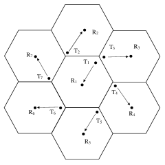
Figure 1: Multicell cellular system

Distances between different receivers and transmitters are shown in Table 2. It should be noted that the channel matrix between any pair of transmitter $i$ and receiver $j$ is a matrix with dimension of $m_{j}\times n_{i}$. In the experiments, we assume $m_{j}=m$ for all $j\in\{1,\ldots,7\}$ $n_{i}=n$ for all $i\in\{1,\ldots,7\}$. As mentioned before, $p_{max}$ is the maximum average transmitted power in units of energy per transmission. In the experiments, the transmitters have a maximum power of $1$ decibels of the measured power referenced to one milliwatt (dBm).

Table 2: Distance matrix (in terms of kilometer)

	R1	R2	R3	R4	R5	R6	R7
T1	0.8944	1.0143	1.0568	1.1020	1.0143	1.0568	1.1020
T2	1.0143	0.8944	1.0568	2.1079	2.6940	2.6677	1.9964
T3	1.1020	1.9011	0.8944	1.0143	2.1079	2.7265	2.7203
T4	1.9964	2.6159	1.9493	0.8944	1.1020	2.1056	2.7620
T5	2.5635	2.6940	2.6677	1.9964	0.8944	1.0568	2.1079
T6	2.5270	2.1079	2.7265	2.7203	1.9011	0.8944	1.0143
T7	1.9011	1.1020	2.1056	2.7620	2.6159	1.9493	0.8944

We investigate the robustness of A-M-SMD algorithm under imperfect feedback. To simulate imperfections, the elements of $Z_{i,t}$ are generated as zero-mean circularly symmetric complex Gaussian random variables with variance equal to $\sigma$. To demonstrate the performance of the methods in this section, we employ the following gap function $Gap(X)$ which is equal to zero for a strong solution.

Definition 3 (A gap function).

Define the following function $Gap:\mathcal{X}\rightarrow\mathbb{R}$

$$Gap(X)=\underset{Z\in\mathcal{X}}{\sup}\ \textnormal{tr}\!\left((X-Z)^{T}F(X)\right),\quad\text{for all}~{}X\in\mathcal{X}.$$ (47)

In the following lemma, we provide some properties of the Gap function. The proof can be find in Appendix.

Lemma 14 (Properties of the Gap function).

The function $Gap(X)$ given by Definition 3 is a well-defined gap function, in other words, $(i)$ $Gap(X)$ is nonnegative for all $X\in\mathcal{X}$; and $(ii)$ $X^{*}$ is a strong solution to Problem (4) iff $Gap({X^{*}})=0$.

The algorithms are run for a fixed number of iterations $T$. We plot the gap function for different number of transmitter antennas ($n$) and receiver antennas ($m$). We also plot the gap function for different values of $\sigma$ including $0.5,1,5$. We use MATLAB to run the algorithms and CVX software to solve the optimization Problem (47). Computational experiments are performed using the same PC running on an Intel Core i5-520M 2.4 GHz processor with 4 GB RAM.

6.3 Averaging and Non-averaging Matrix Stochastic Mirror Descent methods

First, we look into the first 100 iterations in one sample path to see the impact of averaging on the initial performance of matrix stochastic mirror descent (M-SMD) algorithm. Figure 2 compares the performance of averaging stochastic mirror descent (A-M-SMD) algorithm with M-SMD in the first 100 iterations. The pair of $(n,m)$ denotes the number of transmitter and receiver antennas. The vertical axis displays the logarithm of gap function (47) while the horizontal axis displays the iteration number. In these plots, the blue (dash-dot) and black (solid) curves correspond to the M-SMD and A-M-SMD algorithms, respectively. We observe in Figure 2 that A-M-SMD algorithm outperforms the M-SMD in most of the experiments. Importantly, A-M-SMD is significantly more robust with respect to: (i) the imperfections and uncertainty ($\sigma$); and (ii) problem size (the number of transmitter and receiver antennas). Then, we run both A-M-SMD algorithm and M-SMD for $T=4000$ iterations and plot their performance in Figure 3. In this figure, the vertical axis displays the logarithm of expected gap function (47) while the horizontal axis displays the iteration number. The expectation is taken over $Z_{t}$, we repeat the algorithm for $10$ sample paths and obtain the average of the gap function. For comparison purposes, we also plot the performance of M-SMD and A-M-SMD algorithms starting from a different initial point with a better gap function value. This point is obtained by running the algorithm for 400 iterations and saving the best solution $X$ to (47) and its corresponding $Y$. In these plots, the blue (dash-dot) and magenta (solid diamond) curves correspond to the M-SMD with the initial solution $X_{0}=X_{0}^{1}=\mathbf{I}_{n}/n$ and $X_{0}=X_{0}^{2}=X_{400}$ respectively, and the black (solid) and red (dash-dot triangle) curves display the A-M-SMD algorithm with the initial solution $X_{0}=X_{0}^{1}=\mathbf{I}_{n}/n$ and $X_{0}=X_{0}^{2}=X_{400}$ respectively. As it can be seen in Figure 3, A-M-SMD outperforms M-SMD in all experiments. In particular, A-M-SMD is significantly more robust with respect to (i) the imperfections ($\sigma$); and (ii) problem size. It is also observed that A-M-SMD converges to the strong solution with rate of convergence of $\mathcal{O}(1/T)$ while M-SMD does not converge for larger values of $\sigma$. Moreover, from Figure 3, it is evident that the A-M-SMD has better performance compared to M-SMD irrespective to the initial solution.

$(n,m)$	$\sigma=0.5$	$\sigma=1$	$\sigma=5$
(2,4)
(4,2)
(4,4)

Figure 2: Comparison of M-SMD and A-M-SMD w.r.t. problem size ($n,m$) and uncertainty ($\sigma$) for 100 iterations

$(n,m)$	$\sigma=0.5$	$\sigma=1$	$\sigma=5$
(2,4)
(4,2)
(4,4)

Figure 3: Comparison of M-SMD and A-M-SMD w.r.t. initial point ($X_{0}$), problem size ($n,m$), and uncertainty ($\sigma$) for 4000 iterations

Figure 4: Comparison of stability of M-SMD and A-M-SMD in terms of users’ objective function $R_{i}$ for $i=2,4,6$

Stability of M-SMD and A-M-SMD: To compare the stability of two methods, we also plot the expected objective function value $R_{i}$ against the iteration number in Figure 4. Here, we choose $n=m=4$ and $\sigma=10$. The algorithm is repeated for $10$ sample paths and the average of objective function is obtained. Each plot represents the performance of both algorithms for one specific player $i\in\{1,\ldots,7\}$. As an example, the first plot compares the stability of A-M-SMD (black solid curve) and M-SMD (blue dash-dot curve) for the first user. It can be seen that for all players, the A-M-SMD algorithm converges to a strong solution very fast while the M-SMD does not converge and oscillates significantly.

$(n,m)$	$\sigma=0.5$	$\sigma=1$	$\sigma=5$
(2,4)
(4,2)
(4,4)

Figure 5: Comparison of M-SMD, A-M-SMD and MEL w.r.t. problem size ($n,m$), uncertainty ($\sigma$), and regularization parameter ($\lambda$) for 4000 iterations

6.4 Matrix Exponential Learning

Mertikopoulos et al. (2017) proved the convergence of matrix exponential learning (MEL) algorithm under strong stability of mapping $F$ assumption while, in practice, this assumption might not hold for the games and VIs. We proved the convergence of A-M-SMD without assuming strong stability. For comparison purposes, we need to regularize the mapping $F$ by adding the gradient of a strongly convex function to it. Doing so, we obtain a strongly stable mapping (Facchinei and Pang (2007), Chapter 2). Let $\|A\|_{F}$ denote the Frobenius norm of a matrix $A$ which is defined as $\|A\|_{F}=\sqrt{\textnormal{tr}\!\left(A^{T}A\right)}=\sqrt{\sum_{u}\sum_{v}|[A]_{uv}|^{2}}$ (Golub and Van Loan (2012)). In the following Lemma, we show that the function $\frac{1}{2}\|A\|_{F}^{2}$ is strongly convex.

Lemma 15.

The function $h(A)=\frac{1}{2}\|A\|_{F}^{2}$ is strongly convex with parameter 1, i.e.,

$$\frac{1}{2}\|B\|_{F}^{2}\geq\frac{1}{2}\|A\|_{F}^{2}+\textnormal{tr}\!\left(\nabla^{T}_{A}h(A)(B-A)\right)+\frac{1}{2}\|A-B\|_{F}^{2}.$$ (48)

The proof of Lemma 15 can be found in Appendix.

Note that $\nabla\frac{\lambda}{2}\|X\|_{F}^{2}=\lambda X$. Therefore, to regularize the mapping $F$, we need to add the term $\lambda X$ to it and consequently, the mapping $F^{\prime}=F+\lambda X$ is different from the original $F$. It should be noted for small values of $\lambda$, the algorithm converges very slowly. On the other hand, the solution which is obtained by using large values of $\lambda$ may be far from the solution to the original problem. Hence, we need to find a reasonable value of $\lambda$. For this reason, we tried three different values including $0.1,0.5,1$. Note that the difference between MEL and M-SMD algorithm is adding the term $\lambda X$ to the mapping $F$.

For each experiment, the algorithm is run for $T=4000$ iterations. We apply the well-known harmonic stepsize $\eta_{t}=\frac{1}{\sqrt{t}}$ for A-M-SMD and M-SMD, and harmonic stepsize $\eta_{t}=\frac{1}{t}$ for MEL. Figure 5 demonstrates the performance of A-M-SMD, M-SMD and MEL algorithms in terms of logarithm of expected value of gap function (47). The expectation is taken over $Z_{t}$, we repeat the algorithm for $10$ sample paths and obtain the average of gap function. In these plots, the blue (dash-dot) and black (solid) curves correspond to the M-SMD and A-M-SMD algorithms, respectively, the magenta (solid diamond), red (circle dashed) and brown (dashed) curves display MEL algorithm with $\lambda=0.1,0.5$ and $1$. As can be seen in Figure 5, A-M-SMD algorithm outperforms the M-SMD and MEL algorithms in all experiments. It is evident that MEL algorithm converge slowly but faster than M-SMD. Comparing three versions of MEL algorithm which apply large, moderate or small value of regularization parameter $\lambda$, it can be seen that MEL is not robust w.r.t this parameter.

7 Concluding Remarks

We consider multi-agent optimization problems on semidefinite matrix spaces. We develop mirror descent methods where we choose the distance generating function to be defined as the quantum entropy. These first-order single-loop methods include a mirror descent incremental subgradient (M-MDIS) method for minimizing a convex function that consists of sum of component functions and an averaging matrix stochastic mirror descent (A-M-SMD) method for solving Cartesian stochastic variational inequality problems under monotonicity assumption of the mapping. We show that the iterate generated by M-MDIS algorithm converges asymptotically to the optimal solution and derive a non-asymptotic convergence rate. We also prove that A-M-SMD method converges to a weak solution of the CSVI with rate of ${\cal O}(1/\sqrt{t})$. Our numerical experiments performed on a wireless communication network display that the A-M-SMD method is significantly robust w.r.t. the problem size and uncertainty.

8 Appendix

We make use of the following lemma in some proofs.

Lemma 16.

Let $[X]_{uv}$ denotes the elements of matrix $X$. If we rewrite matrices $X$, $Z$ and $\nabla_{{X}}f({X})$ as vectors $x=\left([X]_{11},\ldots,[X]_{nn}\right)^{T}$, $z=\left([z]_{11},\ldots,[z]_{nn}\right)^{T}$, and $\nabla f({x})=\left([\nabla_{{X}}f({X})]_{11},\ldots,[\nabla_{{X}}f({X})]_{nn}\right)^{T}$ respectively, it is trivial that

$$(z-{x})^{T}\nabla f({x})=\sum_{u}\sum_{v}[(Z-X)]_{uv}[\nabla_{X}f(X)]_{uv}=\textnormal{tr}\!\left((Z-{X})^{T}\nabla_{{X}}f({X})\right),$$

where the last inequality follows by relation $\textnormal{tr}\!\left(A^{T}B\right)=\sum_{u}\sum_{v}[{A}]_{uv}[B]_{uv}$.

Proof of Lemma 3:

($\Rightarrow$) Assume $\widetilde{X}^{*}$ is optimal to Problem (14). Assume by contradiction, there exists some $\hat{Z}\in\mathcal{B}$ such that $\textnormal{tr}\!\left((\hat{Z}-\widetilde{X}^{*})^{T}\nabla_{\widetilde{X}}f(\widetilde{X}^{*})\right)<0$. Since $f$ is continuously differentiable, by the first-order Taylor expansion, for all sufficiently small $0<\alpha<1$, we have

$$f(\widetilde{X}^{*}+\alpha(\hat{Z}-\widetilde{X}^{*}))=f({X}^{*})+\textnormal{tr}\!\left((\hat{Z}-\widetilde{X}^{*})^{T}\nabla_{\widetilde{X}}f(\widetilde{X}^{*})\right)+o(\alpha)<f({X}^{*}),$$

following the hypothesis $\textnormal{tr}\!\left((\hat{Z}-\widetilde{X}^{*})^{T}\nabla_{\widetilde{X}}f(\widetilde{X}^{*})\right)<0$. Since $\mathcal{B}$ is convex and $X^{*},~{}\hat{Z}\in\mathcal{B}$, we have $\widetilde{X}^{*}+\alpha(\hat{Z}-\widetilde{X}^{*})\in\mathcal{B}$ with smaller objective function value than the optimal matrix $\widetilde{X}^{*}$. This is a contradiction. Therefore, we must have $\textnormal{tr}\!\left((Z-\widetilde{X}^{*})^{T}\nabla_{\widetilde{X}}f(\widetilde{X}^{*})\right)\geq 0$ for all $Z\in\mathcal{B}$.
($\Leftarrow$) Now suppose that $\widetilde{X}^{*}\in\mathcal{B}$ and $\textnormal{tr}\!\left((Z-\widetilde{X}^{*})^{T}\nabla_{\widetilde{X}}f(\widetilde{X}^{*})\right)\geq 0$ for all $Z\in\mathcal{B}$. Since $f$ is convex and by Lemma 16, we have

$$f(\widetilde{X}^{*})+\textnormal{tr}\!\left((Z-\widetilde{X}^{*})^{T}\nabla_{\widetilde{X}}f(\widetilde{X}^{*})\right)\leq f(Z),\quad\text{for all}\quad Z\in\mathcal{B},$$

which implies for all $Z\in\mathcal{B}$,

$$f(Z)-f(\widetilde{X}^{*})\geq\textnormal{tr}\!\left((Z-\widetilde{X}^{*})^{T}\nabla_{\widetilde{X}}f(\widetilde{X}^{*})\right)\geq 0,$$

where the last inequality follows by the hypothesis. Since $\widetilde{X}^{*}\in\mathcal{B}$, it follows that $\widetilde{X}^{*}$ is optimal.

Proof of Lemma 7:

We use induction to prove (35). It is trivial that it holds for $t=0$, since $\overline{X}_{i,0}={X}_{i,0}$. Assume (35) holds for $t$. From (34), $\Gamma_{t}=\sum_{k^{\prime}=0}^{t}\eta_{k^{\prime}}$ which results in $\overline{X}_{i,t}=\frac{\sum_{k=0}^{t}\eta_{k}X_{i,k}}{\Gamma_{t}}$. From (34), we have

$$\overline{X}_{i,t+1}:=\frac{\Gamma_{t}\overline{X}_{i,t}+\eta_{t+1}{X}_{i,t+1}}{\Gamma_{t+1}}=\frac{\sum_{k=0}^{t}\eta_{k}X_{i,k}+\eta_{t+1}{X}_{i,t+1}}{\Gamma_{t+1}}=\frac{\sum_{k=0}^{t+1}\eta_{k}X_{i,k}}{\sum_{k^{\prime}=0}^{t+1}\eta_{k}^{\prime}}.$$

Proof of Lemma 8:

Using the Fenchel coupling definition,

$$H({X},{Y}+{Z})=\omega({X})+\omega^{*}({Y}+Z)-\textnormal{tr}\!\left({X^{T}}({Y}+Z)\right).$$ (49)

By strong convexity of $\omega$ w.r.t. trace norm (Lemma 1) and using duality between strong convexity and strong smoothness Kakade et al. (2009), $\omega^{*}$ is 1-strongly smooth w.r.t. the spectral norm, i.e., $\omega^{*}({Y}+Z)\leq\omega^{*}({Y})+\textnormal{tr}\!\left(Z^{T}\nabla\omega^{*}({Y})\right)+\|Z\|^{2}_{2}.$ By plugging this inequality into (49) we have

$$H({X},{Y}+{Z}) \leq\omega({X})+\omega^{*}({Y})+\textnormal{tr}\!\left(Z^{T}\nabla\omega^{*}({Y})\right)+\|Z\|^{2}_{2}-\textnormal{tr}\!\left({X^{T}}{Y}\right)-\textnormal{tr}\!\left({X^{T}}{Z}\right)$$

$$=H({X},{Y})+\textnormal{tr}\!\left(Z^{T}(\nabla\omega^{*}({Y})-{X})\right)+\|Z\|^{2}_{2},$$

where in the last relation, we used (36).

Proof of Lemma 10:

We use the following definitions in the proof.

Definition 4 (Matrix convex function).

Let $\mathbb{C}^{n}$ be the complex vector space.

An arbitrary matrix $A\in\mathbb{H}_{m}$ is nonnegative if $(Ay)^{\dagger}y\geq 0$ for all $y\in\mathbb{C}^{n}$.

For $A,B\in\mathbb{H}_{m}$ we write $A\geq B$ if $A-B$ is nonnegative.

A function $f:\mathbb{H}_{m}\rightarrow\mathbb{H}_{n}$ is convex if $f(\lambda A+(1-\lambda)B)\leq\lambda f(A)+(1-\lambda)f(B)$, for all $0\leq\lambda\leq 1$.

A function $f:\mathbb{H}_{m}\rightarrow\mathbb{H}_{n}$ is called matrix monotone increasing if $A\geq B$ implies $f(A)\geq f(B)$ (Watkins (1974)).

A function $f:\mathbb{H}_{m}\rightarrow\mathbb{R}$ is called matrix monotone increasing if $A\geq B$ implies $f(A)\geq f(B)$ (Kwong (1989)).

Proof.

Assume that $X,Z\in\mathbb{H}_{m}$, and $0\leq\lambda\leq 1$. By convexity of $\mathbb{H}_{m}$, we have $\lambda X+(1-\lambda)Z\in\mathbb{H}_{m}$, and from concavity of $g$, we have

$$g(\lambda X+(1-\lambda)Z)\geq\lambda g(X)+(1-\lambda)g(Z).$$ (50)

Since $h$ is matrix monotone increasing and by Definition 4(e), we get

$$h\left(g(\lambda X+(1-\lambda)Z)\right)\geq h\left(\lambda g(X)+(1-\lambda)g(Z)\right)\geq\lambda h(g(X))+(1-\lambda)h(g(Z)),$$ (51)

where the last inequality follows from concavity of $h$. Therefore,

$$h\left(g(\lambda X+(1-\lambda)Z)\right)\geq\lambda h(g(X))+(1-\lambda)h(g(Z)),$$ (52)

and we conclude that $f$ is a concave function. ∎

Proof of Lemma 12:

By convexity of $f$ and by Lemma 16, we have for arbitrary $X,Z\in\mathcal{X}$

$$f({Z})+\textnormal{tr}\!\left((X-{Z})^{T}\nabla_{{Z}}f({Z})\right)\leq f(X).$$

By choosing the points in reverse, we also have

$$f({X})+\textnormal{tr}\!\left((Z-{X})^{T}\nabla_{{X}}f({X})\right)\leq f(Z).$$

Summing the above inequalities, we get

$$f(Z)+f({X})+\textnormal{tr}\!\left((X-{Z})^{T}\nabla_{{Z}}f({Z})\right)+\textnormal{tr}\!\left((Z-{X})^{T}\nabla_{{X}}f({X})\right)\leq f(X)+f(Z),$$

and using the fact that $\textnormal{tr}\!\left(A+B\right)=\textnormal{tr}\!\left(A\right)+\textnormal{tr}\!\left(B\right)$, we get the desired result.

Proof of Lemma 14:

$(i)$ For an arbitrary $X\in\mathcal{X}$, we have

$$Gap(X)=\underset{Z\in\mathcal{X}}{\sup}\ \textnormal{tr}\!\left((X-Z)^{T}F(X)\right)\geq\textnormal{tr}\!\left((X-A)^{T}F(X)\right),\quad\text{for all}~{}A\in\mathcal{X}.$$

For $A=X$, the above inequality suggests that $Gap(X)\geq\textnormal{tr}\!\left((X-X)^{T}F(X)\right)=0$ implying that the function $Gap(X)$ is nonnegative for all $X\in\mathcal{X}$.
$(ii)$ Assume $X^{*}$ is a strong solution. By definition of VI($\mathbf{\mathcal{X}},F$) and relation (4), we have

$$\textnormal{tr}\!\left(({X^{*}}-X)^{T}F(X^{*})\right)\leq 0,\quad\text{for all}~{}X\in\mathbf{\mathcal{X}}$$

which implies

$$Gap({X^{*}})=\underset{X\in\mathcal{X}}{\sup}\ \textnormal{tr}\!\left(({X^{*}}-X)^{T}F(X^{*})\right)\leq 0,\quad\text{for all}~{}X\in\mathbf{\mathcal{X}}.$$

On the other hand, from Lemma 14$(i)$, we get $Gap({X^{*}})\geq 0$. We conclude that for any strong solution ${X^{*}}$, we have $Gap({X^{*}})=0$. Conversely, assume that there exist an $X$ such that $Gap(X)=0$. Therefore, $\underset{Z\in\mathcal{X}}{\sup}\ \textnormal{tr}\!\left((X-Z)^{T}F(X)\right)=0$ which implies $\textnormal{tr}\!\left((X-Z)^{T}F(X)\right)\leq 0$ for all $Z\in\mathcal{X}$. Equivalently, we get $\textnormal{tr}\!\left((Z-X)^{T}F(X)\right)\geq 0$ for all $Z\in\mathcal{X}$ implying $X$ is a strong solution.

Proof of Lemma 15:

For an arbitrary matrix $A$, we have $\nabla_{A}\textnormal{tr}\!\left(A^{T}A\right)=A$ (Athans and Schweppe (1965), page 32). That being said and using the definition of Frobenius norm, we have

$$\frac{1}{2}\|A\|_{F}^{2}+\textnormal{tr}\!\left(\nabla^{T}_{A}h(A)(B-A)\right)+\frac{1}{2}\|A-B\|_{F}^{2}=$$

$$\frac{1}{2}\|A\|_{F}^{2}+\textnormal{tr}\!\left({A}^{T}(B-A)\right)+\frac{1}{2}\textnormal{tr}\!\left((A-B)^{T}(A-B)\right)=$$

$$\frac{1}{2}\|A\|_{F}^{2}+\textnormal{tr}\!\left({A}^{T}(B-A)\right)+\frac{1}{2}\textnormal{tr}\!\left(A^{T}A-B^{T}A-A^{T}B+B^{T}B\right)=$$

$$\frac{1}{2}\|A\|_{F}^{2}+\textnormal{tr}\!\left(A^{T}B-A^{T}A\right)+\frac{1}{2}\textnormal{tr}\!\left(A^{T}A-B^{T}A-A^{T}B+B^{T}B\right)=$$

$$\frac{1}{2}\|A\|_{F}^{2}+\frac{1}{2}\textnormal{tr}\!\left(A^{T}B\right)-\frac{1}{2}\textnormal{tr}\!\left(A^{T}A\right)-\frac{1}{2}\textnormal{tr}\!\left(B^{T}A\right)+\frac{1}{2}\textnormal{tr}\!\left(B^{T}B\right)=$$

$$\frac{1}{2}\|A\|_{F}^{2}+\frac{1}{2}\textnormal{tr}\!\left(A^{T}B\right)-\frac{1}{2}\|A\|_{F}^{2}-\frac{1}{2}\textnormal{tr}\!\left(A^{T}B\right)+\frac{1}{2}\|B\|_{F}^{2}=\frac{1}{2}\|B\|_{F}^{2}.$$

Therefore, the inequality (48) holds in equality and we conclude that $h(A)$ is strongly convex with parameter 1.

References

• Athans and Schweppe (1965) Athans, Michael, Fred C Schweppe. 1965. Gradient matrices and matrix calculations. Tech. rep., Massachusetts Inst of Tech Lexington Lab.
• Beck (2017) Beck, A. 2017. First-Order Methods in Optimization. Series: MOS-SIAM Series on Optimization, Philadelphia, PA.
• Bertsekas (2011) Bertsekas, Dimitri P. 2011. Incremental proximal methods for large scale convex optimization. Mathematical programming 129 163.
• Bertsekas (2015) Bertsekas, Dimitri P. 2015. Incremental aggregated proximal and augmented Lagrangian algorithms. arXiv preprint arXiv:1509.09257 .
• Bien and Tibshirani (2011) Bien, Jacob, Robert J Tibshirani. 2011. Sparse estimation of a covariance matrix. Biometrika 98 807–820.
• Boţ and Böhm (2018) Boţ, Radu Ioan, Axel Böhm. 2018. An incremental mirror descent subgradient algorithm with random sweeping and proximal step. Optimization 1–18.
• Boyd and Vandenberghe (2004) Boyd, Stephen, Lieven Vandenberghe. 2004. Convex optimization. Cambridge university press.
• Carlen (2010) Carlen, Eric. 2010. Trace inequalities and quantum entropy: an introductory course. Entropy and the Quantum 529 73–140.
• Chang et al. (2015) Chang, Tsung-Hui, Mingyi Hong, Xiangfeng Wang. 2015. Multi-agent distributed optimization via inexact consensus admm. IEEE Trans. Signal Processing 63 482–497.
• Chen et al. (2017) Chen, Yunmei, Guanghui Lan, Yuyuan Ouyang. 2017. Accelerated schemes for a class of variational inequalities. Mathematical Programming 165 113–149.
• de Pillis (1967) de Pillis, John. 1967. Linear transformations which preserve hermitian and positive semidefinite operators. Pacific Journal of Mathematics 23 129–137.
• Defazio et al. (2014) Defazio, Aaron, Francis Bach, Simon Lacoste-Julien. 2014. Saga: A fast incremental gradient method with support for non-strongly convex composite objectives. Advances in neural information processing systems. 1646–1654.
• Durham et al. (2012) Durham, Joseph W, Antonio Franchi, Francesco Bullo. 2012. Distributed pursuit-evasion without mapping or global localization via local frontiers. Autonomous Robots 32 81–95.
• Facchinei and Pang (2003) Facchinei, Francisco, Jong-Shi Pang. 2003. Finite-dimensional variational inequalities and complementarity problems. Vols. I,II. Springer Series in Operations Research, Springer-Verlag, New York.
• Facchinei and Pang (2007) Facchinei, Francisco, Jong-Shi Pang. 2007. Finite-dimensional variational inequalities and complementarity problems. Springer Science & Business Media.
• Fazel et al. (2001) Fazel, Maryam, Haitham Hindi, Stephen P Boyd. 2001. A rank minimization heuristic with application to minimum order system approximation. Proceedings of the American Control Conference, vol. 6. IEEE, 4734–4739.
• Golub and Van Loan (2012) Golub, Gene H, Charles F Van Loan. 2012. Matrix computations, vol. 3. JHU Press.