EUROPEAN ORGANIZATION FOR NUCLEAR RESEARCH (CERN)

​​​ CERN-EP-2018-336 LHCb-PAPER-2018-039

Dalitz plot analysis of the ${{D}^{+}}\!\rightarrow{{K}^{-}}{{K}^{+}}{{K}^{+}}$ decay

LHCb collaboration

The resonant structure of the doubly Cabibbo-suppressed decay ${{D}^{+}}\!\rightarrow{{K}^{-}}{{K}^{+}}{{K}^{+}}$ is studied for the first time. The measurement is based on a sample of $pp$-collision data, collected at a centre-of-mass energy of 8 TeV with the LHCb detector and corresponding to an integrated luminosity of 2$\mbox{\,fb}^{-1}$. The amplitude analysis of this decay is performed with the isobar model and a phenomenological model based on an effective chiral Lagrangian. In both models the S-wave component in the $K^{-}K^{+}$ system is dominant, with a small contribution of the $\phi(1020)$ meson and a negligible contribution from tensor resonances. The $K^{+}K^{-}$ scattering amplitudes for the considered combinations of spin (0,1) and isospin (0,1) of the two-body system are obtained from the Dalitz plot fit with the phenomenological decay amplitude.

Published in JHEP 04 (2019) 063.

© 2024 CERN for the benefit of the LHCb collaboration. CC-BY-4.0 licence.

 

1 Introduction

The theoretical treatment of weak decays of charm mesons is very challenging. The charm quark is not light enough for the reliable application of chiral perturbation theory, which is successfully applied in predictions of kaon decays. The charm quark is also not heavy enough for the reliable application of the factorisation approach and heavy-quark expansion tools, as used in predictions of properties of b hadrons. The description of charm meson decays relies on approximate symmetries and phenomenological models. For such models, the knowledge of branching fractions and the resonant structures, in the case of multi-body decays, are key inputs. In this paper, the first determination of the resonant structure of the doubly Cabibbo-suppressed decay ${{D}^{+}}\!\rightarrow{{K}^{-}}{{K}^{+}}{{K}^{+}}$ is presented. The analysis is based on a data sample of $pp$ collisions collected with the LHCb detector, corresponding to an integrated luminosity of 2 $\mbox{\,fb}^{-1}$ at a centre-of-mass energy of 8 TeV. The determination of the resonant structure of this decay is complementary to the recent LHCb measurement of its branching fraction [1], based on the same data set.

The amplitude analysis of the ${{D}^{+}}\!\rightarrow{{K}^{-}}{{K}^{+}}{{K}^{+}}$ decay is performed using two methods. The Dalitz plot is fitted with the isobar model, in which the decay amplitude is a coherent sum of resonant and nonresonant amplitudes [2]. The Dalitz plot is also fitted with a phenomenological model derived from an effective chiral Lagrangian with resonances [3]. This phenomenological model, referred to as the multi-meson model, or Triple-M, includes the effects of coupled channels — $\pi\pi$, $K^{+}K^{-}$, $\pi\eta$, $\eta\eta$ and $\rho\pi$ — in the final state interactions (FSI), in four considered combinations of spin J and isospin I ($J\!=\!0,1$; $I\!=\!0,1$). Given the small phase space of the ${{D}^{+}}\!\rightarrow{{K}^{-}}{{K}^{+}}{{K}^{+}}$ decay and the lack of tensor resonances with significant coupling to $K^{+}K^{-}$, the contribution from D-wave is expected to be suppressed.

An additional motivation for the Dalitz plot analysis of the ${{D}^{+}}\!\rightarrow{{K}^{-}}{{K}^{+}}{{K}^{+}}$ decay is to obtain the $K^{+}K^{-}$ scattering amplitudes. Most information currently available on $\pi\pi$ and $K\pi$ scattering is obtained indirectly from meson-nucleon interactions [4, 5, 6]. In the regime where the momentum transferred to the nucleon is small enough, the interaction is assumed to be dominated by the one-pion-exchange amplitude. The asymptotically free incoming meson interacts with a virtual pion, resulting in what is generally referred as $\pi\pi$ and $K\pi$ scattering data. The resulting $\pi\pi\rightarrow\pi\pi$ and $K\pi\rightarrow K\pi$ phase shifts are affected by ambiguities and large systematic uncertainties. The $\pi\pi\rightarrow K{\kern 1.99997pt\overline{\kern-1.99997ptK}{}}$ scattering was studied both in $\pi p$ and $\pi n$ reactions [7, 8], and in $p\bar{p}$ annihilation at rest [9]. For the $K{\kern 1.99997pt\overline{\kern-1.99997ptK}{}}\rightarrow K{\kern 1.99997pt\overline{\kern-1.99997ptK}{}}$ scattering, no meson-nucleon data exists.

Three-body decays of $D$ mesons into kaons and pions are an interesting alternative for light-meson spectroscopy, as they are complementary to the meson-nucleon reactions. Large data sets from the $B$-factories and LHCb exist for these decays. However, it is necessary to isolate the physics of two-body systems from the rich dynamics of three-body decays, which involve the weak decay of the $c$ quark, the formation of the mesons and their FSI. This is achieved with the Triple-M decay amplitude, in which these three stages are included. The FSI are described in terms of the $K^{+}K^{-}$ scattering amplitudes for the considered spin-isospin combinations, allowing the determination of these amplitudes from a fit to the ${{D}^{+}}\!\rightarrow{{K}^{-}}{{K}^{+}}{{K}^{+}}$ Dalitz plot.

This paper is organised as follows. A brief description of the LHCb detector is presented in Sec. 2. The signal selection is presented in Sec. 3. In Sec. 4, the efficiency determination and background model are discussed. The formalism for the Dalitz plot fit is presented in Sec. 5. In Sec. 6, the results of the fit with the isobar model are presented, whilst the results of the Dalitz plot fit with the Triple-M amplitude are presented in Sec. 7. Systematic uncertainties are discussed in Sec. 8. A summary and the conclusions are presented in Sec. 9.

2 Detector and simulation

The LHCb detector [10, 11] is a single-arm forward spectrometer covering the pseudorapidity range $2<\eta<5$, designed for the study of particles containing $b$ or $c$ quarks. The detector includes a high-precision tracking system consisting of a silicon-strip vertex detector surrounding the $pp$ interaction region, a large-area silicon-strip detector located upstream of a dipole magnet with a bending power of about $4{\mathrm{\,Tm}}$, and three stations of silicon-strip detectors and straw drift tubes placed downstream of the magnet. The tracking system provides a measurement of the momentum, $p$, of charged particles with a relative uncertainty that varies from 0.5% at low momentum to 1.0% at 200$\mathrm{\,Ge\kern-1.00006ptV}$. The minimum distance of a track to a primary vertex (PV), the impact parameter (IP), is measured with a resolution of $(15+29/\mbox{$p_{\rm T}$}){\,\upmu\rm m}$, where $p_{\rm T}$ is the component of the momentum transverse to the beam, in GeV. Different types of charged hadrons are distinguished using information from two ring-imaging Cherenkov detectors [12]. Photons, electrons and hadrons are identified by a calorimeter system consisting of scintillating-pad and pre-shower detectors, an electromagnetic and a hadronic calorimeter. Muons are identified by a system composed of alternating layers of iron and multi-wire proportional chambers.

The online event selection is performed by a trigger, which consists of a hardware stage, based on information from the calorimeter and muon systems, followed by a software stage, which applies a full event reconstruction. At the hardware trigger stage, events are required to have a muon with high $p_{\rm T}$ or a hadron, photon or electron with high transverse energy in the calorimeters. The software trigger is divided into two parts. The first employs a partial reconstruction of the candidates from the hardware trigger and a cut-based selection. In the second stage, a full event reconstruction is applied and various dedicated algorithms are used in the selection of specific decays. In this analysis, a dedicated algorithm is used to select ${{D}^{+}}\!\rightarrow{{K}^{-}}{{K}^{+}}{{K}^{+}}$ decay candidates.

In the simulation, $pp$ collisions are generated using Pythia [13, *Sjostrand:2007gs] with a specific LHCb configuration [15]. Decays of hadronic particles are described by EvtGen [16], in which final-state radiation is generated using Photos [17]. The interaction of the generated particles with the detector, and its response, are implemented using the Geant4 toolkit [18, *Agostinelli:2002hh] as described in Ref. [20].

3 Candidate selection

The ${{D}^{+}}\!\rightarrow{{K}^{-}}{{K}^{+}}{{K}^{+}}$ decay candidates are selected offline with requirements that exploit the decay topology by combining three charged particles identified as kaons according to particle-identification (PID) criteria. These particles must form a good-quality decay vertex, detached from the PV. The PV is chosen as that with the smallest value of $\chi^{2}_{\rm IP}$, where $\chi^{2}_{\rm IP}$ is defined as the difference in the vertex-fit $\chi^{2}$ of the PV reconstructed with and without the particle under consideration, in this case the ${D}^{+}$ candidate. The selection of candidates is based on the distance between the PV and the ${D}^{+}$ decay vertex (the flight distance); the IP of the ${D}^{+}$ candidate; the angle between the reconstructed ${D}^{+}$ momentum vector and the vector connecting the PV to the decay vertex; the $\chi^{2}$ of the ${D}^{+}$ decay vertex fit; the distance of closest approach between any two final-state tracks; and the momentum, the transverse momentum and the $\chi^{2}_{\rm IP}$ of the ${D}^{+}$ candidate and of its decay products. The invariant mass of the ${D}^{+}$ candidate is required to be within the interval 1820–1920$\mathrm{\,Me\kern-1.00006ptV}$. In order to suppress the contamination from $D^{+}_{s}\rightarrow K^{-}K^{+}\pi^{+}\pi^{0}$ decays, where the neutral pion is not reconstructed and the charged pion is misidentified as a kaon, more stringent PID requirements are applied to the kaon candidates with the same charge.

A boosted decision tree (BDT) multivariate classifier [21, 22] is used to further reduce the combinatorial background. In order to keep the selection efficiency uniform over the Dalitz plot, the BDT uses only the quantities related to the $D^{+}$ candidate described above. The BDT is trained using simulated ${{D}^{+}}\!\rightarrow{{K}^{-}}{{K}^{+}}{{K}^{+}}$ decays for the signal, and data from the invariant-mass intervals 1820–1840$\mathrm{\,Me\kern-1.00006ptV}$ and 1900–1920$\mathrm{\,Me\kern-1.00006ptV}$ for the background. After the application of all selection requirements, approximately 0.5% of the events include more than one signal candidate. All candidates are retained for further analysis.

The invariant-mass spectrum of the selected ${{D}^{+}}\!\rightarrow{{K}^{-}}{{K}^{+}}{{K}^{+}}$ sample is shown in Fig. 1. To fit the invariant-mass distribution, the signal probability density function (PDF) is modeled by a sum of two Gaussian functions with a common mean and independent widths that are free parameters. The signal model is validated with simulation. The background PDF is parameterised by an exponential function. The fitted PDF is overlaid with the mass distribution in Fig. 1. For the Dalitz plot analysis, only candidates within the range 1861.4–1879.5 $\mathrm{\,Me\kern-1.00006ptV}$ are considered. This interval corresponds to four times the effective mass resolution, and contains 111 thousand candidates, of which $(90.45\pm 0.07)\%$ correspond to signal.

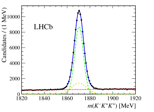
Figure 1: Invariant-mass spectrum of the $K^{-}K^{+}K^{+}$ candidates with the fit result overlaid (solid blue line). The orange and green dashed lines indicate the two Gaussian functions representing the signal and the red dashed line is the background.

The Dalitz plot of the candidates in the signal region is shown in the left side of Fig 2. The particle ordering is such that the kaon with charge opposite to that of the $D^{+}$ meson is always particle 1, and the same-sign kaons are randomly assigned particles 2 and 3, i.e. $D^{+}\rightarrow K^{-}(p_{1})K^{+}(p_{2})K^{+}(p_{3})$, where $p_{i}$ are the four-momenta. The Dalitz plot is represented in terms of the square of the invariant masses of the two $K^{-}K^{+}$ combinations, $s_{12}\equiv(p_{1}+p_{2})^{2}$ and $s_{13}\equiv(p_{1}+p_{3})^{2}$. Throughout this paper, the symbol $s_{K^{-}K^{+}}$ is used to represent the invariant mass squared of both $K^{-}K^{+}$ combinations. These Lorentz-invariant quantities are computed constraining the invariant mass of the candidate to the known $D^{+}$ mass [23]. An accumulation of candidates is visible at $s_{K^{-}K^{+}}$ $\sim$1.04$\mathrm{\,Ge\kern-1.00006ptV^{2}}$ which corresponds to the $\phi(1020)K^{+}$ component. The difference in the number of candidates in the regions of the Dalitz plot above and below 1.55$\mathrm{\,Ge\kern-1.00006ptV^{2}}$ (regions I and II in the left side of Fig. 2, respectively) is caused by interference between the $\phi(1020)K^{+}$ and S-wave amplitudes. This interference also shifts the position of the peaks of the $s_{K^{-}K^{+}}$ distributions in the two regions. These two effects are better illustrated in the projections of the Dalitz plot shown in the right side of Fig. 2.

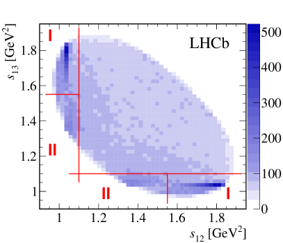
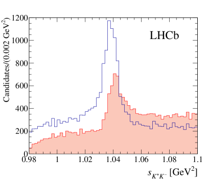
Figure 2: (left) Dalitz plot of the selected sample, including background. (right) Dalitz plot projections for candidates from regions I (blue) and II (red), above and below $s_{K^{-}K^{+}}\!=\!1.5$$\mathrm{\,Ge\kern-1.00006ptV^{2}}$. The interference between the S- and P-wave amplitudes cause the asymmetry in the number of candidates in the two regions, as well as the shift in the peak position. Both figures include all candidates in the selected mass range.

4 Efficiency and background model

4.1 Efficiency variation over the Dalitz plot

In the fit to the Dalitz plot distribution, the variation of the total efficiency across the phase space must be taken into account. The total efficiency is determined from a combination of simulation and methods based on data, and includes the geometrical acceptance of the detector and the reconstruction, selection, PID and trigger efficiencies.

The geometrical acceptance, reconstruction and selection efficiencies are obtained from simulation. The PID efficiency of each $D^{+}$ candidate is determined by multiplying the efficiencies for each of the final-state kaons. The PID efficiencies for the kaons are evaluated from calibration samples of $D^{*+}\rightarrow D^{0}(\rightarrow K^{-}\pi^{+})\pi^{+}$ decays [24] and depend on the particle momentum, pseudorapidity and event charged-particle multiplicity. The trigger efficiency is obtained from simulation, with a correction factor determined from data to account for the small mismatch between the performance of the trigger in data and simulation.

The total efficiency distribution is a two-dimensional histogram with $14\times 14$ uniform bins. A two-dimensional cubic spline is used to smooth this distribution to avoid binning discontinuities, yielding the high-resolution histogram ($300\times 300$ uniform bins), shown in Fig. 3. This histograms is used to weight the signal PDF in the Dalitz plot fit. The binning scheme of the efficiency histogram is a source of systematic uncertainty.

4.2 Background model

The background model is built from the inspection of the mass sidebands of the ${{D}^{+}}\!\rightarrow{{K}^{-}}{{K}^{+}}{{K}^{+}}$ signal. The Dalitz plots of candidates from both sidebands, 1820–1840$\mathrm{\,Me\kern-1.00006ptV}$ and 1900–1920$\mathrm{\,Me\kern-1.00006ptV}$, are very similar, with a clear peaking structure, corresponding to random $\phi(1020)K^{+}$ combinations over a smooth distribution.

The Dalitz plot variables are computed from the four-momenta determined by a $D^{+}$ mass constrained fit. This constraint implies an unique boundary of the Dalitz plot, regardless of the value of the invariant mass of the three-kaon system. It also improves the mass resolution of signal candidates, but has the effect to distort and shift any structure present in the Dalitz plot of the background candidates in the sidebands. This effect depends strongly on the invariant mass of the three-kaon system and prevents the determination of the background model from a two-dimensional parameterisation of the Dalitz plots from the sidebands. An alternative method is used instead. Each $m(K^{-}K^{+}K^{+})$ sideband is divided into slices of 5$\mathrm{\,Me\kern-1.00006ptV}$. For each slice, the projections onto the $s_{K^{+}K^{-}}$ axis are fitted using a relativistic Breit–Wigner for the $\phi(1020)$ component (with floated mass and width) and a phase-space distribution. The latter serves as a proxy for both the smooth component spread across the Dalitz plot and the projection of the $\phi$ candidates appearing in the other $s_{K^{+}K^{-}}$ combination. The fraction of the $\phi(1020)$ component is nearly constant in both sidebands, indicating that the background composition is independent of $m(K^{-}K^{+}K^{+})$. A linear interpolation is used to obtain the fraction of peaking background in the signal region and is found to be (20.67$\pm$0.28)%.

The fit to the $s_{K^{+}K^{-}}$ projection has the limitation of being less sensitive to the distribution near the $K^{+}K^{-}$ threshold. The inspection of the Dalitz plot sidebands shows that the smooth background component has more candidates at low values of $s_{K^{+}K^{-}}$ and fewer at low values of $s_{K^{+}K^{+}}\equiv(p_{2}+p_{3})^{2}$, indicating that this smooth distribution is not uniform over the phase space. A model for the smooth component of the background is built assuming a sum of two contributions, random $f_{0}(980)K^{+}$ candidates and a constant amplitude, with equal proportions. The relative fractions of these two terms in the smooth component is treated as a source of systematic uncertainty.

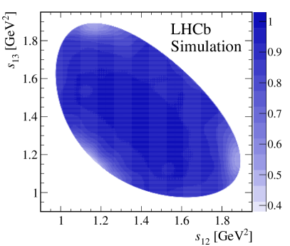
Figure 3: Total efficiency, normalised to unity, for the ${{D}^{+}}\!\rightarrow{{K}^{-}}{{K}^{+}}{{K}^{+}}$ signal over the Dalitz plot, including the geometrical acceptance and the reconstruction, selection, PID and trigger efficiencies.

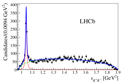
Figure 4: Projection onto $s_{K^{+}K^{-}}$ of $K^{-}K^{+}K^{+}$ candidates with invariant mass in the range 1820–1830 MeV.

A high-resolution normalised histogram ($300\times 300$ uniform bins) is used in the Dalitz plot fit to represent the background PDF, and is shown in Fig. 5. This histogram is produced from a large simulated sample, using a PDF in which the peaking and smooth components are added incoherently with the estimated relative fractions and weighted by the efficiency function.

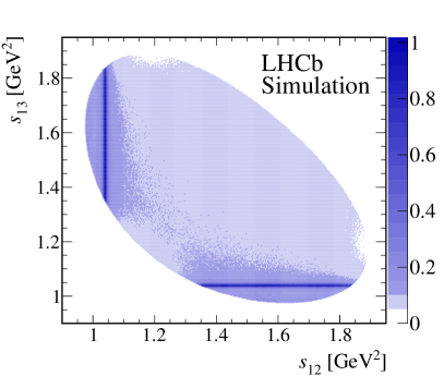
Figure 5: High-resolution histogram representing the background model used in the Dalitz plot fits.

5 The Dalitz plot fit procedure

The ${{D}^{+}}\!\rightarrow{{K}^{-}}{{K}^{+}}{{K}^{+}}$ decays are studied through an unbinned maximum-likelihood fit to the observed Dalitz plot distribution. The total PDF is constructed as a sum of signal and background components, and the likelihood function is given by

$$\mathcal{L}=\prod^{N_{\rm cand}}f_{\rm S}\times S_{\rm PDF}(s_{12},s_{13})+(1-f_{\rm S})\times B_{\rm PDF}(s_{12},s_{13}),$$ (1)

where $N_{\rm cand}$ is the total number of candidates and $f_{S}$ is the fraction of signal candidates in the sample, as obtained from the $m(K^{-}K^{+}K^{+})$ fit described in Sec. 3. The background PDF, $B_{\rm PDF}(s_{12},s_{13})$, is described in Sec. 4.2.

The normalised signal PDF is written in terms of the total decay amplitude ${\mathcal{T}}(s_{12},s_{13})$,

$$S_{\rm PDF}(s_{12},s_{13})=\frac{1}{N_{\rm S}}{\left|\mathcal{T}(s_{12},s_{13})\right|}^{2}\varepsilon(s_{12},s_{13}),$$ (2)

where $\varepsilon(s_{12},s_{13})$ is the detection efficiency, described in Sec. 4.1. The normalisation factor, $N_{\rm S}$, is given by

$$N_{\rm S}=\int{\rm d}s_{12}\ {\rm d}s_{13}\left|\mathcal{T}(s_{12},s_{13})\right|^{2}\varepsilon(s_{13},s_{13}).$$ (3)

For any given model, the amplitude ${\mathcal{T}}(s_{12},s_{13})$ depends on a set of parameters that are floated in the fit. The optimum values for these parameters are determined by minimizing the quantity $-2\ln\mathcal{L}$ using the MINUIT package [25].

In order to compare the fit results of a given model to the Dalitz plot distribution in data, a large simulated sample is generated according to the model, including background and efficiency, normalised to the total number of data candidates. Since there are two identical kaons, the folded Dalitz plot is used, represented as $s_{K^{+}K^{-}}^{\rm high}$ versus $s_{K^{+}K^{-}}^{\rm low}$, which are respectively the higher and the lower values among $s_{12}$ and $s_{13}$. The Dalitz plot distribution is divided into 1024 bins with approximately 110 candidates each and the normalised residuals are computed as

$$\Delta_{i}=\frac{(N_{\rm pred}^{i}-N_{\rm obs}^{i})}{\sigma_{i}},$$ (4)

where, for each bin $i$, $N_{\rm pred}^{i}$ is the predicted number of candidates from the model, $N_{\rm obs}^{i}$ is the number of candidates in the data sample, and $\sigma_{i}$ is the statistical uncertainty from data and simulation added in quadrature. The sum of the square values of $\Delta_{i}$ over all bins is the total $\chi^{2}$ and is used as a metric to compare fit results with different models.

6 Dalitz plot analysis with the isobar model

In the isobar model, the decay amplitude is written as a coherent sum of a constant nonresonant (NR) component and intermediate resonant amplitudes,

$${\cal T}(s_{12},s_{13})=c_{\rm NR}+\sum_{k}c_{k}T_{k}(s_{12},s_{13}).$$ (5)

Each resonant amplitude, $T_{k}$, is given by a product of Blatt–Weisskopf penetration factors [26], $F_{D}^{L}$ and $F_{R}^{L}$, accounting for the finite size of the $D^{+}$ meson and the resonance, respectively, the spin amplitude, $\mathcal{S}$, accounting for the conservation of angular momentum, and a function, $M_{R}$, describing the resonance lineshape, which is either a relativistic Breit–Wigner (Eq. A.2) or a Flatté lineshape (Eq. A.4). The Zemach formalism [27] is used for the spin amplitude $\mathcal{S}$. Details of each of these factors are given in Appendix A. Since there are two identical kaons in the final state, the resonant amplitudes are Bose-symmetrised,

$$T_{k}(s_{12},s_{13})=F_{D}^{L}(s_{12})F_{R}^{L}(s_{12})\,\times\,\mathcal{S}(s_{12},s_{13})\,\times\,M_{R}(s_{12})+(2\leftrightarrow 3).$$ (6)

The fit parameters are the complex coefficients $c_{\rm NR}=a_{\rm NR}e^{i\delta_{\rm NR}}$ and $c_{k}=a_{k}e^{i\delta_{k}}$. The results are expressed in terms of the magnitude and phase of the complex coefficient for each component, and the corresponding fit fractions. The fit fractions are computed by integrating the squared modulus of the corresponding amplitude over the phase space, and dividing by the integral of the total amplitude squared,

$${\rm FF}_{k}=\frac{\int{\rm d}s_{12}\ {\rm d}s_{13}\ |c_{k}\ T_{k}(s_{12},s_{13})|^{2}}{\int{\rm d}s_{12}\ {\rm d}s_{13}\ \left|\sum_{i}c_{i}\ T_{i}(s_{12},s_{13})\right|^{2}}.$$ (7)

The sum of fit fractions for all components is, in general, different from 100% due to the presence of interference; it is less than 100% in the case of net constructive interference or higher than 100% otherwise.

6.1 Signal models

For the ${{D}^{+}}\!\rightarrow{{K}^{-}}{{K}^{+}}{{K}^{+}}$ decay amplitude, contributions from following resonances are possible: the isoscalars $f_{0}(980)$, $f_{0}(1370)$ and $f_{0}(1500)$; the isovectors $a_{0}(980)$ and $a_{0}(1450)$; the vector $\phi(1020)$; the tensor $f_{2}(1270)$. Contributions from resonances with spin greater than one are suppressed due to the small phase space of the ${{D}^{+}}\!\rightarrow{{K}^{-}}{{K}^{+}}{{K}^{+}}$ decay. In the case of the $f_{2}(1270)$ state, a further suppression is expected due to its small branching fraction to $K^{-}K^{+}$, $(4.6\pm 0.4)$% [23]. The relatively narrow $f^{\prime}_{2}(1525)$ state is neglected since it is well beyond the phase space.

Various combinations of the nonresonant and the possible resonant amplitudes are considered. All models studied contain the $\phi(1020)K^{+}$, which is chosen as the reference amplitude, fixing the phase convention and setting the scale for the magnitudes. The models tested differ by the composition of the S-wave. Near the $K^{+}K^{-}$ threshold, both the $a_{0}(980)$ and $f_{0}(980)$ resonances can contribute. Similarly, at higher $K^{+}K^{-}$ invariant mass, contributions from several scalar resonances are possible.

The $\phi(1020)$ mass and width are fixed to the known values [23]; for the $f_{0}(980)$ state, a Flatté lineshape is used, with parameters from the BESII collaboration [28].

6.2 Results

The simplest model that describes the data, referred to as model A, consists of three intermediate components: $\phi(1020)K^{+}$, $f_{0}(980)K^{+}$, and $f_{0}(1370)K^{+}$. As the $f_{0}(1370)$ state has large uncertainties on its mass and width [23], these parameters are allowed to float in the fit. Its contribution can also be interpreted, within the isobar formalism, as an effective representation for the overlap of two or more broad structures at high $K^{-}K^{+}$ invariant mass.

Further addition of scalar states does not improve the fit quality significantly, creates more complex interference effects, and provides a very similar description of the lineshape and phase behaviour of the total S-wave. For example, in model B, a constant nonresonant contribution is added to the resonant amplitudes of model A. The resulting fit quality is essentially unchanged, with the total $\chi^{2}/{\rm ndof}$ being 1.15 and 1.14 for models A and B, respectively. A similar situation occurs in model C, which has the same amplitudes as in model B plus the $a_{0}(980)K^{+}$ component. In this model, the contribution of the $f_{0}(1370)$ is found to be negligible and the value of $\chi^{2}/{\rm ndof}$ is 1.16. Table 1 summarizes the fit results for these three models. The total S-wave fit fraction includes the interference terms between the various S-wave components. In all cases, the total S-wave in the $K^{+}K^{-}$ system is dominant, a notable feature also observed in other three-body $D$ decays with a pair of identical particles in the final state, such as the $D^{+}\rightarrow K^{-}\pi^{+}\pi^{+}$ and $D^{+}_{(s)}\rightarrow\pi^{-}\pi^{+}\pi^{+}$ decays[23]. The contribution from the $f_{2}(1270)K^{+}$ component is also tested and found to be consistent with zero in all models.

Since model A is the simplest model describing all the general features of the observed Dalitz plot distribution, it is chosen as the baseline result for the fit with the isobar model. The projections of the Dalitz plot, with the model A fit result overlaid, are shown in Fig. 6. The green dashed line represents the phase-space distribution, weighted by the efficiency, evidencing the presence of at least one broad, scalar contribution not consistent with a uniform distribution.

Table 1: Results from the ${{D}^{+}}\!\rightarrow{{K}^{-}}{{K}^{+}}{{K}^{+}}$ Dalitz plot fit with the isobar models A, B and C. Magnitudes, $|c_{k}|$ , phases, $\arg(c_{k})$ (in degrees), and fit fractions (in %) are given with statistical uncertainties only.

		Model A		Model B		Model C
$\phi(1020)K^{+}$	Magnitude	1 [fixed]		1 [fixed]		1 [fixed]
	Phase	0 [fixed]		0 [fixed]		0 [fixed]
	Fraction	6.17 $\pm$	0.47	6.40 $\pm$	0.47	6.40 $\pm$	0.48
$f_{0}(980)K^{+}$	Magnitude	3.12 $\pm$	0.10	2.64 $\pm$	0.08	2.84 $\pm$	0.13
	Phase	$-58.9$ $\pm$	4.9	$-36.5$ $\pm$	7.6	$-25.9$ $\pm$	8.4
	Fraction	23.7 $\pm$	3.0	17.7 $\pm$	2.1	20.4 $\pm$	1.5
$f_{0}(1370)K^{+}$	Magnitude	3.46 $\pm$	0.46	2.33 $\pm$	0.35	–
	Phase	13.1 $\pm$	7.7	42 $\pm$	10	–
	Fraction	25.4 $\pm$	5.0	18.7 $\pm$	1.5	–
	$f_{0}(1370)$ mass [$\mathrm{\,Ge\kern-1.00006ptV}$ ]	1.422 $\pm$	0.015	1.401 $\pm$	0.009	–
	$f_{0}(1370)$ width [$\mathrm{\,Ge\kern-1.00006ptV}$ ]	0.324 $\pm$	0.038	0.178 $\pm$	0.031	–
NR	Magnitude	–		8.8 $\pm$	1.3	11.7 $\pm$	1.8
	Phase	–		$-5.5$ $\pm$	6.5	$-39.0$ $\pm$	4.4
	Fraction	–		18.4 $\pm$	5.9	32.7 $\pm$	8.2
$a_{0}(980)K^{+}$	Magnitude	–		–		5.9 $\pm$	0.4
	Phase	–		–		48.5 $\pm$	3.0
	Fraction	–		–		53.5 $\pm$	7.4
	S-wave fraction	92 $\pm$	11	91 $\pm$	13	93 $\pm$	12
	Fractions sum	55.4 $\pm$	5.9	61.2 $\pm$	6.4	113 $\pm$	11

Table 2: Fit results with model A, given in terms of the magnitudes $|c_{k}|$, phases, $\arg(c_{k})$ (in degrees), and fit fractions (in %). For each measurement, the first uncertainty is statistical, the second systematic and the third is a systematic uncertainty due to model.

Component	Magnitude				Phase [deg.]				Fraction (%)
$\phi(1020)K^{+}$	1.0 [fixed]				0.0 [fixed]				6.17 $\pm$	0.47  $\pm$	0.19  $\pm$	0.41
$f_{0}(980)K^{+}$	3.12 $\pm$	0.10  $\pm$	0.13  $\pm$	0.33	$-58.9$ $\pm$	4.9  $\pm$	2.3  $\pm$	2.0	23.7 $\pm$	3.0  $\pm$	2.1  $\pm$	3.3
$f_{0}(1370)K^{+}$	3.46 $\pm$	0.46  $\pm$	0.32  $\pm$	0.73	13.1 $\pm$	7.7  $\pm$	1.6  $\pm$	3.2	25.4 $\pm$	5.0  $\pm$	3.4  $\pm$	3.8
sum									55.4 $\pm$	5.9  $\pm$	0.4  $\pm$	0.6

The distribution of the normalised residuals $\Delta_{i}$ over the Dalitz plot is shown in the left plot of Fig. 7, and their distribution is consistent with a normal Gaussian, as shown in the right plot of Fig. 7. In Table 2 the results including the systematic and model uncertainties, as discussed in Sec. 8, are presented.

The squared modulus and phase of the S-wave amplitude from model A are shown in Fig. 8 as a function of the $K^{+}K^{-}$ mass, with total uncertainties represented as bands. For comparison, the corresponding central results for models B and C are overlaid. Although the S-wave composition is different for these models, the total S-wave description is essentially the same, evidencing that the isobar model fails to disentangle the individual contributions. The $f_{0}(1370)$ parameters are found to be $m_{0}=1.422\pm 0.015\pm 0.009\pm 0.028$$\mathrm{\,Ge\kern-1.00006ptV}$ and $\Gamma_{0}=0.324\pm 0.038\pm 0.018\pm 0.038$$\mathrm{\,Ge\kern-1.00006ptV}$, where the first uncertainties are statistical and the second systematic.

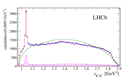
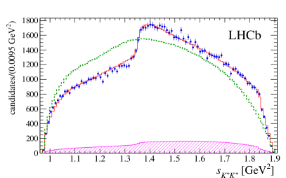
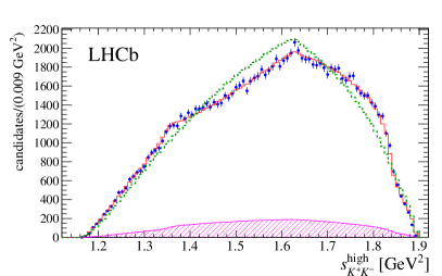
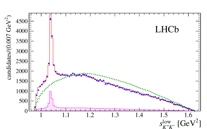
Figure 6: Projections of the Dalitz plot onto (top left) $s_{K^{+}K^{-}}$, (top right) $s_{K^{+}K^{+}}$, (bottom left) $s_{K^{+}K^{-}}^{\rm high}$ and (bottom right) $s_{K^{+}K^{-}}^{\rm low}$ axes, with the fit result with model A overlaid (red histogram). The histogram in magenta represents the contribution from the background, whereas the dashed green line is the phase-space distribution weighted by the efficiency.

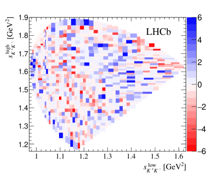
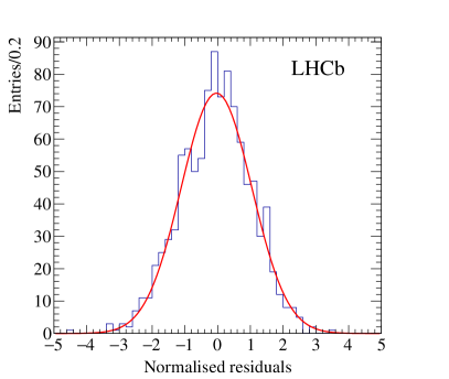
Figure 7: (left) Normalised residuals $\Delta_{i}$ across the Dalitz plot, from the result of isobar fit. (right) Distribution of the normalised residuals with the fit result overlaid. The distribution is fitted with a Gaussian function and the fit result is consistent with the standard normal distribution.

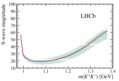
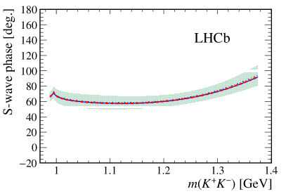
Figure 8: (left) Magnitude and (right) phase of the total S-wave from the result of the Dalitz plot fit with the isobar model. The black line corresponds to model A and the green band represents the statistical and systematic uncertainties added in quadrature. For comparison, the results of models B and C are shown as the blue solid and dashed thick red lines. Uncertainties on the S-wave magnitude and phase for models B and C are similar to those from model A and are not shown.

7 Dalitz plot analysis with the Triple-M amplitude

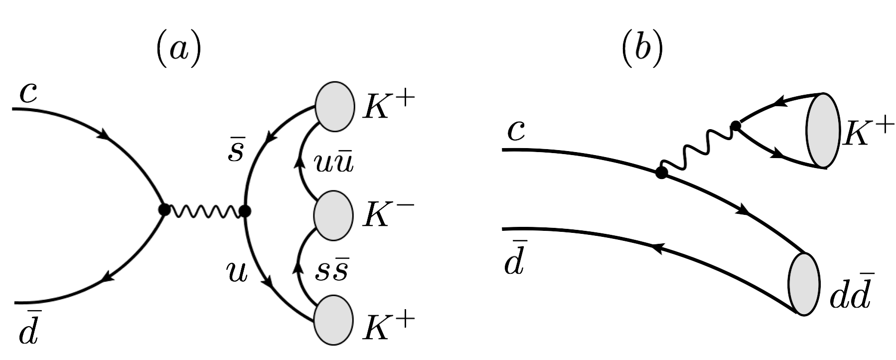
Figure 9: Diagrams representing the two quark-level topologies for the ${{D}^{+}}\!\rightarrow{{K}^{-}}{{K}^{+}}{{K}^{+}}$ decay. In the Triple-M [3], diagram ($a$) is assumed to be the dominant mechanism of the decay, whereas diagram ($b$) is suppressed since the production of a $K^{+}K^{-}$ pair from a $d\bar{d}$ pair requires rescattering.

The basic hypothesis of the Triple-M is the dominance of the annihilation diagram shown in Fig. 9(a). The ${{D}^{+}}\!\rightarrow{{K}^{-}}{{K}^{+}}{{K}^{+}}$ decay can also proceed via the diagram in Fig. 9(b), but in this case a $K^{+}K^{-}$ pair could only be produced from the $d\bar{d}$ pair through rescattering, since charged kaons have no $d$-valence quark. The same holds for the production of the $\phi(1020)$ meson which is essentially an $s\bar{s}$ state [23].

Assuming the annihilation diagram is the dominant mechanism for the ${{D}^{+}}\!\rightarrow{{K}^{-}}{{K}^{+}}{{K}^{+}}$ decay, the Triple-M amplitude is a product of two axial-vector currents,

$$\langle K^{-}K^{+}K^{+}|\mathcal{T}|D^{+}\rangle=-\left[\frac{G_{F}}{\sqrt{2}}\,\sin^{2}\theta_{C}\right]\langle K^{-}K^{+}K^{+}|A_{\mu}|0\rangle\langle 0|A_{\mu}|D^{+}\rangle\ ,$$ (8)

where $G_{F}$ is the Fermi decay constant, $\theta_{C}$ is the Cabibbo angle and $A^{\mu}$ are the axial currents. The weak vertex is $\langle\,0\,|A_{\mu}|\,D^{+}(P)\rangle=-i\,\sqrt{2}\,f_{D}\,P_{\mu}$, where $P=p_{1}+p_{2}+p_{3}\,$ is the $D^{+}$ four-momentum and $f_{D}$ is the $D^{+}$ decay constant.

In the Triple-M, the three-kaon system can be produced in two ways, as illustrated in the diagrams in Fig. 10. Diagram (a) represents the production of the three kaons directly from the weak vertex, whereas in diagram (b) two of the three kaons result from the decay of a bare intermediate resonance. Final state interactions are introduced in diagrams (c) and (d). The full black circles indicate the unitarised scattering amplitudes, $A_{K^{+}K^{-}}^{JI}$, representing the scattering $ab\rightarrow K^{+}K^{-}$ with the coupled channels $ab=K^{+}K^{-},\ \pi\pi,\ \eta\pi$ and $\eta\eta$ in a well-defined spin (J ) and isospin (I ) state. The nonresonant component corresponds to diagram (a). Due to the existence of two identical kaons, diagrams (b), (c) and (d) are symmetrised. As in the isobar analysis, contributions of D-wave are expected to be very small and are not included.

The Triple-M decay amplitude therefore has five components,

$$\mathcal{T}=T_{\rm NR}+\sum_{J,I}T^{JI},\hskip 17.07182ptJ,I=0,1.$$ (9)

The free parameters in the Triple-M amplitude are the couplings and masses of the chiral Lagrangian. There are four couplings, $c_{d},\ c_{m},\ \tilde{c}_{d},\ \tilde{c}_{m}$ in the scalar part, contributing to $T^{00}$ and $T^{01}$ terms; two masses, $m_{So},\ m_{S1}$, for the scalar-isoscalar, $T^{00}$ contribution and one, $m_{a_{0}}$, in the scalar-isovector $T^{01}$ components; one coupling, $G_{V}$, for the vector components, $T^{10}$ and $T^{11}$, and one mass, $m_{\phi}$, in the vector-isoscalar component. In the fit to the data, the combination $G_{\phi}\equiv G_{V}\sin\theta_{\omega-\phi}/F$ is used as free parameter, where $\theta_{\omega-\phi}$ is the $\omega-\phi$ mixing angle. The parameter $F$ is the $SU(3)$ pseudoscalar decay constant, common to all components. For convenience, the formulae of the various components of the Triple-M amplitude are reproduced from Ref. [3] in Appendix B.

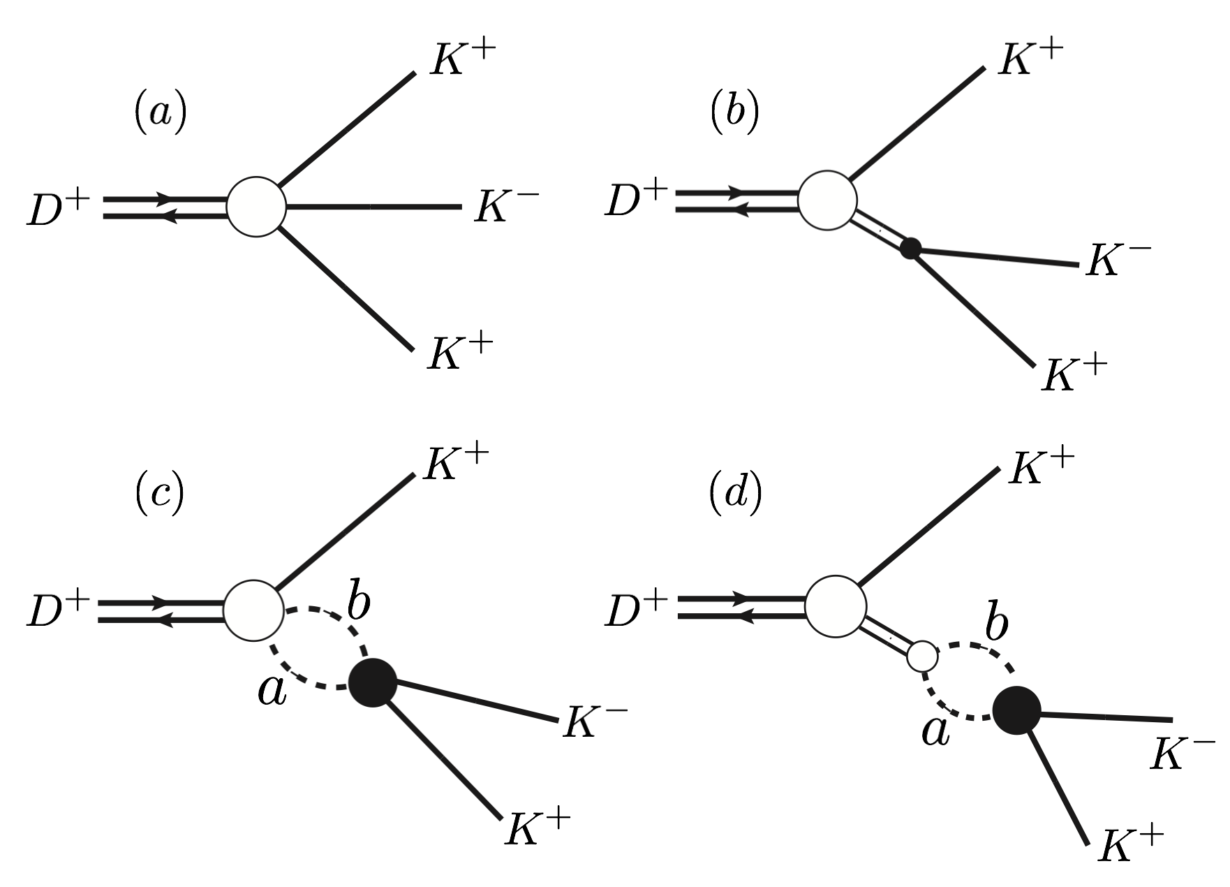
Figure 10: Diagrams contributing to the amplitude $\mathcal{T}$ for the decay $D^{+}\rightarrow K^{-}\,K^{+}\,K^{+}$: (a) the final state kaons are produced directly from the weak vertex; (b) a bare resonance is produced directly from the weak vertex; (c) particles produced at the weak vertex undergo final state interactions; (d) final state interactions endow finite widths to the resonances. The full circle represents the unitary $ab\rightarrow K^{+}K^{-}$ scattering amplitude with angular momentum $J$ and isospin $I$, and $ab=K\overline{K},\ \pi\pi,\ \eta\pi$ and $\eta\eta$.

Equation 9 resembles that of the isobar model, but there are several significant differences. The free parameters in the Triple-M amplitude are real quantities from the chiral Lagrangian. Some of these parameters appear in different spin-isospin components of the model. In the isobar model the free parameters are the complex coefficients $c_{k}$, from which the individual contributions of the resonances are determined. In the Triple-M amplitude, the relative contributions of the various components are fixed by theory. The nonresonant component is usually represented by an empirical constant in fits with the isobar model. In the Triple-M amplitude, it is a function of the Dalitz plot coordinates and is fully determined by chiral symmetry.

7.1 Fit results

The optimum values of the Triple-M parameters are determined by an unbinned maximum-likelihood fit, as described in Sec. 5. The fitted values of the Triple-M parameters are listed in Table 3, with statistical and systematic uncertainties.

The quality of the fit with the Triple-M amplitude is tested with the metric defined in Eq. 4. The value of $\chi^{2}/{\rm ndof}$ is 1.12. The projections of the Dalitz plot onto the $s_{K^{+}K^{-}}$ and the $s_{K^{+}K^{+}}$ axes, as well as the projections onto the highest and lowest invariant masses squared of the two $K^{+}K^{-}$ combinations, $s_{K^{+}K^{-}}^{\rm high}$ and $s_{K^{+}K^{-}}^{\rm low}$, are shown in Fig. 11, with the fit result superimposed. The projections indicate that the model is in good agreement with the data. The distribution of the normalised residuals over the Dalitz plot is shown in the right panel of Fig. 12. The distribution of normalised residuals, shown in the left panel of Fig. 12, is consistent with a normal Gaussian.

Table 3: Results of the $D^{+}\rightarrow K^{-}K^{+}K^{+}$ Dalitz plot fit with the Triple-M amplitude.

parameter	value
$F$	$94.3^{+2.8}_{-1.7}$ $\pm$	1.5$\mathrm{\,Me\kern-1.00006ptV}$
$m_{a_{0}}$	$947.7^{+5.5}_{-5.0}$ $\pm$	6.6$\mathrm{\,Me\kern-1.00006ptV}$
$m_{S_{o}}$	$992.0^{+8.5}_{-7.5}$ $\pm$	8.6$\mathrm{\,Me\kern-1.00006ptV}$
$m_{S_{1}}$	$1330.2^{+5.9}_{-6.5}$ $\pm$	5.1$\mathrm{\,Me\kern-1.00006ptV}$
$m_{\phi}$	$1019.54^{+0.10}_{-0.10}$ $\pm$	0.51$\mathrm{\,Me\kern-1.00006ptV}$
$G_{\phi}$	$0.464^{+0.013}_{-0.009}$ $\pm$	0.007 0
$c_{d}$	$-78.9^{+4.2}_{-2.7}$ $\pm$	1.9$\mathrm{\,Me\kern-1.00006ptV}$
$c_{m}$	$106.0^{+7.7}_{-4.6}$ $\pm$	3.3$\mathrm{\,Me\kern-1.00006ptV}$
$\tilde{c}_{d}$	$-6.15^{+0.55}_{-0.54}$ $\pm$	0.19$\mathrm{\,Me\kern-1.00006ptV}$
$\tilde{c}_{m}$	$-10.8^{+2.0}_{-1.5}$ $\pm$	0.4$\mathrm{\,Me\kern-1.00006ptV}$

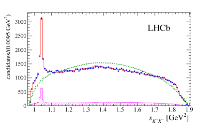
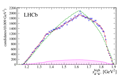
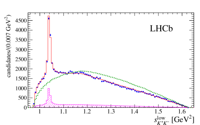
Figure 11: Projections of the Dalitz plot onto (top left) $s_{K^{+}K^{-}}$, (top right) $s_{K^{+}K^{+}}$, (bottom left) $s_{K^{+}K^{-}}^{\rm high}$ and (bottom right) $s_{K^{+}K^{-}}^{\rm low}$ axes, with the fit result with the Triple-M amplitude superimposed, whereas the dashed green line is the phase space distribution weighted by the efficiency. The magenta histogram represents the contribution from the background.

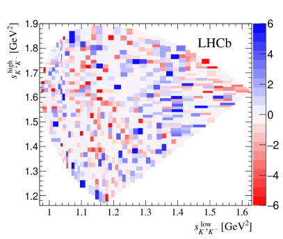
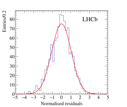
Figure 12: (left) Two-dimensional distribution of the normalised residuals for the Triple-M fit. (right) Distribution of normalised residuals of each bin.

7.2 Interpretation

The resonance masses in the Triple-M are introduced in the denominators, D, of Eqs. B.21–B.24, where the functions M are imaginary and proportional to interaction kernels which contain the bare masses of the effective chiral Lagrangian, $m_{a_{0}}$, $m_{S_{o}}$, $m_{S_{1}}$ and $m_{\phi}$. The Triple-M amplitude is derived assuming that only the imaginary part of the two-body propagators in Eqs. B.25–B.28 is relevant. In this approximation, the bare masses coincide with the masses of the physical states and the association $m_{S_{o}}=m_{f_{0}(980)}$ and $m_{S_{1}}=m_{f_{0}(1370)}$ can be made. As in the case of the isobar model, the masses in the Triple-M correspond to the values of $s_{K^{+}K^{-}}$ for which the real part of the denominator D of Eqs. B.21–B.24 vanishes. At these values of $s_{K^{+}K^{-}}$, only the imaginary parts of the denominators remain, corresponding to the model prediction for the widths. The denominators D would be very similar to those from the isobar model if no coupled channel was considered. The inclusion of coupled channels is, therefore, the main difference between the Triple-M and Breit–Wigner denominators, resulting in widths with different dynamical content.

7.2.1 Resonant structure

The nonresonant contribution in the Triple-M is a three-body amplitude predicted by chiral symmetry. It can be projected into the S- and P-waves rewriting Eq. B.3 as

$$T_{\rm NR} = \frac{C}{4}\left[\,(m_{D}^{2}-m_{K}^{2}+s_{12})+\,(s_{13}-s_{23})+(m_{D}^{2}-m_{K}^{2}+s_{13})+\,(s_{12}-s_{23})\right]$$ (10)

$$= T_{\rm NR}^{S}+T_{\rm NR}^{P}\;,$$

where $C$ is a constant common to all components of the Triple-M amplitude, and defined in Eq. B.2. The decay amplitude can then be written as the sum of scalar and vector components

$$\mathcal{T}=\left[T^{S}+T^{P}+(2\leftrightarrow 3)\right],$$ (11)

with

$$T^{S}=T_{NR}^{S}+T^{00}+T^{01}\;$$ (12)

and

$$T^{P}=T_{NR}^{P}+T^{11}+T^{10}\;.$$ (13)

The relative contribution of each individual component of the Triple-M amplitude is determined by integrating the modulus squared of each term in the right-hand side of Eq. 9 over the phase space of the ${{D}^{+}}\!\rightarrow{{K}^{-}}{{K}^{+}}{{K}^{+}}$ decay,

$${\rm FF}_{\rm NR}=\frac{\int{\rm d}s_{12}\ {\rm d}s_{13}\ |T_{\rm NR}(s_{12},s_{13})|^{2}}{\int{\rm d}s_{12}\ {\rm d}s_{13}\ \left|\mathcal{T}(s_{12},s_{13})\right|^{2}},\hskip 22.76228pt{\rm FF}^{JI}=\frac{\int{\rm d}s_{12}\ {\rm d}s_{13}\ |T^{JI}(s_{12},s_{13})|^{2}}{\int{\rm d}s_{12}\ {\rm d}s_{13}\ \left|\mathcal{T}(s_{12},s_{13})\right|^{2}}.$$ (14)

Similarly, the S-wave contribution can be determined by the integral over the phase space of the modulus squared of the $T^{S}$ component, defined in Eq. 12, and divided by the integral of the modulus squared of the decay amplitude $\mathcal{T}$. The results are summarised in Table 4. There is a large destructive interference between the two scalar below-threshold states, $a_{0}(980)$ and $f_{0}(980)$, yielding an S-wave contribution of $(94\pm 1)$%. The large $a_{0}(980)/f_{0}(980)$ interference may be, in part, due to the fact that in the $K^{+}K^{-}$ mass spectrum these two states have very similar lineshapes, since only the tails are visible. This large interference is also observed in the fit with the isobar model C, yielding similar fit fractions for the S-wave component. A more accurate determination of the relative contribution of the $a_{0}(980)$ and $f_{0}(980)$ resonances could be obtained from a simultaneous analysis of the $D^{+}\rightarrow\pi^{+}\pi^{-}\pi^{+}$ and $D^{+}\rightarrow\eta\pi^{+}\pi^{0}$. The contribution of the $\phi(1020)$ resonance, $(7.1\pm 0.5)\%$, is consistent to that observed in the fit with the isobar model.

Table 4: Relative fractions (%) of the various components of the Triple-M amplitude. The uncertainties correspond to the combined statistical and systematic uncertainties.

${\rm FF_{NR}}$	${\rm FF}^{00}$	${\rm FF}^{01}$	${\rm FF}^{10}$	${\rm FF}^{11}$	${\rm FF_{S-wave}}$
14 $\pm$ 1	29 $\pm$ 1	131 $\pm$ 2	7.1 $\pm$ 0.9	0.26 $\pm$ 0.01	94 $\pm$ 1

7.2.2 Decay and scattering amplitudes

The phases of the S-wave amplitude, $T^{S}$, and the $K^{+}K^{-}\rightarrow K^{+}K^{-}$ scattering amplitudes, $A^{0I}_{K^{+}K^{-}}$, for the two allowed isospin states, are shown in Fig. 13 as a function of the $K^{+}K^{-}$ invariant mass. The bands correspond to the statistical and systematic uncertainties added in quadrature. The kink in the phase of $T^{S}$ at $m(K^{+}K^{-})\sim 1.25$ GeV is due to the opening of the $\eta\eta$ channel. The curves of Fig. 13 illustrate the difference between decay and scattering amplitudes. The latter, which depends on spin and isospin, is a substructure of the former, which depends only on spin. The expressions of the various scattering amplitudes, derived in Ref. [3], are reproduced in Appendix C.

The physics of two-body scattering is encompassed by the phase shifts and inelasticities. These quantities are obtained from the scattering amplitudes, following the procedure described in Ref. [3]. The phase shifts, $\delta^{JI}_{K^{+}K^{-}}$, and inelasticities $\eta^{JI}_{K^{+}K^{-}}$, are displayed in Fig. 14 for $J\!=\!0$ and $I\!=\!0,1$.

The interpretation of the phase shifts for $K^{+}K^{-}$ scattering is not as straightforward as in the case of elastic scattering, since for both isospin states, the $\pi\pi\rightarrow K^{+}K^{-}$ and $\pi\eta\rightarrow K^{+}K^{-}$ channels are already open at the $K^{+}K^{-}$ threshold. An interesting feature of the results displayed is that the phase variation of $\delta^{00}_{K^{+}K^{-}}$ is monotonic and spans over more than $180^{\circ}$, with a fast variation starting at $m(K^{+}K^{-})\sim 1.4$ GeV, close to the value of $m_{S_{1}}$ and typical of a resonance at high $K^{+}K^{-}$ mass. A fast variation of the phases is observed near threshold for both $\delta^{00}_{K^{+}K^{-}}$ and $\delta^{01}_{K^{+}K^{-}}$, indicating the contribution from the resonances below threshold.

The $\eta\eta$ channel contributes to $T^{00}$ but not to $T^{01}$ and its effect is visible in the bottom left plot of Fig. 14 as a kink at $m(K^{+}K^{-})\sim 1.1$$\mathrm{\,Ge\kern-1.00006ptV}$. As elastic scattering corresponds to $\eta^{JI}=1$, one sees that the isoscalar component becomes significantly more inelastic after the mass of the second scalar resonance.

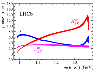
Figure 13: Phase of the $J\!=\!0$ component of the decay amplitude (blue) $T^{S}=T^{00}+T^{01}+T_{\rm NR}^{S}$, compared to the phases of the scattering amplitudes, (red) $A_{K^{+}K^{-}}^{00}$ and (magenta) $A_{K^{+}K^{-}}^{01}$ as a function of the $K^{+}K^{-}$ invariant mass.

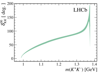
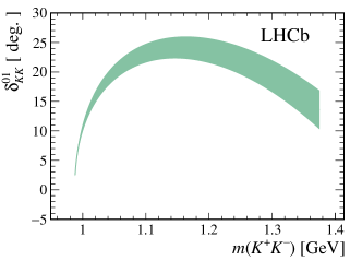
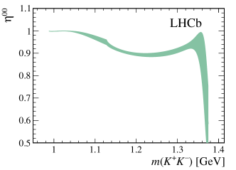
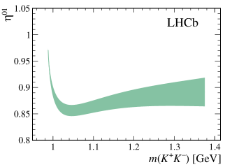
Figure 14: (top) Phase-shifts $\delta^{0I}_{K^{+}K^{-}}$ and (bottom) inelasticities $\eta^{0I}$ as a function of the $K^{+}K^{-}$ invariant mass, for both isospin states.

8 Systematic uncertainties

Sources of systematic uncertainties associated to the background model, to the efficiency correction and to possible biases in the fitting procedure are common to the fits with the isobar model and the Triple-M. They are summarized in Tables 5 and 6, respectively. There is an additional source of systematic uncertainties on the results of the fit with the isobar model due to the uncertainties on the parameters defining the $f_{0}(980)$ lineshape, which are fixed in the fit. This additional uncertainty, quoted separately from the experimental uncertainties, is estimated by repeating the fit varying the parameters $g_{\pi}$, $g_{K}$ and $m_{0}$ of Eq. A.4 by one standard deviation, one at a time, and taking the largest deviation as the systematic uncertainty. The radii of the Blatt–Weisskopf form factors are also fixed in the fit. However, they impacts only the $\phi(1020)K^{+}$ amplitude. Fits with alternative values of these parameters are performed. The tested values of the radii are 4 and 6 GeV^-1, for $F_{D}^{L}$, and 1 and 3 GeV^-1, for $F_{R}^{L}$. Since no significant deviation from the baseline fit is observed, no systematic uncertainty is assigned.

Two types of systematic uncertainties due to the background are investigated. First, the background level is varied according to the uncertainty from the fit to the $K^{-}K^{+}K^{+}$ invariant mass. The data is fitted changing the fraction of the background by $\pm 1\sigma$. No significant change in the fit parameters is found and no systematic uncertainty is assigned. Uncertainties due to the background modelling are also investigated. The background model is built from inspection of the sidebands of the ${{D}^{+}}\!\rightarrow{{K}^{-}}{{K}^{+}}{{K}^{+}}$ signal. It is a combination of a peaking structure and a smooth component. The smooth component corresponds to 80% of the background and is modelled by a sum of a constant term and an $f_{0}(980)K^{+}$ contribution, in equal proportions. A systematic uncertainty due to the modelling of the background is assigned by varying the relative fractions of these two components, fitting the data with these alternative background models and taking the largest variation as systematic uncertainty.

Table 5: Systematic uncertainties (%) on the results of the isobar model fit. For comparison, the statistical uncertainties are listed in the last column.

parameter	binning	sim. stat.	bkg.	total	model	stat.
$|c_{f_{0}(980)}|$	1.0	1.4	3.8	4.2	11	3.0
$\delta_{f_{0}(980)}$	3.1	1.9	1.4	3.9	3.4	8.2
$|c_{f_{0}(1370)}|$	3.5	3.5	7.8	9.2	21	13
$\delta_{f_{0}(1370)}$	9.3	5.2	4.4	12	24	59
$M_{f_{0}(1370)}$	0.1	0.3	0.6	0.7	2.0	1.0
$\Gamma_{f_{0}(1370)}$	3.7	3.0	3.1	5.7	12	12

Table 6: Systematic uncertainties (%) on the results of the Triple-M fit. For comparison, the statistcal uncertainties are listed in the last column.

parameter	binning	sim. stat.	PID	bkg.	fit bias	total	stat.
$F$	0.53	0.07	0.09	1.5	0.11	1.6	1.8
$m_{a_{0}}$	0.54	0.14	-	0.40	0.16	0.70	0.54
$m_{So}$	0.60	0.21	-	0.56	0.21	0.87	0.82
$m_{S1}$	0.16	0.15	-	0.13	0.04	0.26	0.41
$m_{\phi}$	0.002	0.001	-	-	0.002	0.003	0.005
$G_{\phi}$	0.86	0.25	0.02	1.2	0.15	1.5	1.9
$c_{d}$	0.18	0.08	0.09	2.4	0.13	2.4	3.3
$c_{m}$	0.16	0.11	-	2.7	0.10	2.7	4.7
$\tilde{c}_{d}$	0.13	0.15	-	2.6	1.1	3.1	8.8
$\tilde{c}_{m}$	0.19	0.11	0.08	2.8	1.9	3.4	13

Systematic uncertainties are assigned to small biases in the fit using ensembles of 500 simulated samples. Two sets of samples are generated using the Triple-M amplitude and the isobar model, both with the fitted values of the parameters. In the simulations the signal PDFs are weighted by the efficiency function and the background component is included. Each simulated sample is fitted independently, resulting in distributions of fitted values of the parameters and their respective uncertainties. For each parameter, the mean of the distribution of fitted values is compared to the input. The difference is assigned as the systematic uncertainty due to the fit bias. A small bias is observed in the fit with the Triple-M amplitude, whilst no bias is observed in the fit with the isobar model.

The systematic uncertainty associated to the efficiency variation across the Dalitz plot includes the effect of the uncertainties on the PID efficiency and the hardware trigger correction factors, the effect of the finite size of the simulated sample, and the effect of the binning scheme of the efficiency histogram prior to the two-dimensional spline smoothing. The uncertainties on the PID efficiency are due to the finite size of the calibration samples and imply small systematic uncertainties compared to the other sources of systematics, in the fit with the Triple-M amplitude, and negligible uncertainties in the fit with the isobar model. The uncertainty due to the hardware trigger correction factors is found to be negligible. The effect of the finite size of the simulated sample is assessed by generating a set of alternative histograms from the selection efficiency histogram, prior to the hardware trigger correction and the PID efficiency weighting. The content of each bin of the selection efficiency histogram is varied according to a Poisson distribution. For each of these alternative histograms, an efficiency map is produced and used to fit the data. For each parameter, the root mean square of the distribution of fitted values is assigned as a systematic uncertainty. The systematic uncertainty due to the binning scheme of the efficiency map is accessed by varying the number of bins of the final efficiency histogram. The histograms with alternative binnings are fitted by the two-dimensional cubic spline. The data is fitted with these alternative efficiency maps and the largest variation of each parameter is assigned as systematic uncertainty.

9 Summary and conclusions

In this paper, the first Dalitz plot analysis of the doubly Cabibbo-suppressed decay ${{D}^{+}}\!\rightarrow{{K}^{-}}{{K}^{+}}{{K}^{+}}$ is performed. The two goals of the analysis are the determinations of the resonant structure of the decay and the $K^{+}K^{-}$ scattering amplitudes. The resonant structure is studied with two different approaches. In the fit with the isobar model, several variations of the decay amplitude are tested. The Dalitz plot analysis is also performed with the Triple-M [3], which is a model derived from a chiral effective Lagrangian. The Triple-M amplitude has a nonresonant component plus the minimal $SU(3)$ content corresponding to four states, the $\phi(1020)$, the $a_{0}(980)$ and two isoscalar states, identified with the $f_{0}(980)$ and $f_{0}(1370)$ resonances. A good description of the data is achieved with both approaches.

The resonant structure of the ${{D}^{+}}\!\rightarrow{{K}^{-}}{{K}^{+}}{{K}^{+}}$ is largely dominated by the S-wave, with a approximately 7% contribution from the $\phi(1020)K^{+}$ component. The dominance of the S-wave contribution is also observed in other three-body $D^{+}_{(s)}$ decays with a pair of identical particles in the final state, such as the $D^{+}\rightarrow K^{-}\pi^{+}\pi^{+}$ and $D^{+}_{(s)}\rightarrow\pi^{-}\pi^{+}\pi^{+}$ decays[23]. The possibility of determining the individual components of the S-wave, however, is limited by the lack of structures in the Dalitz plot, other than that from the $\phi(1020)$ resonance, and by the fact that the $f_{0}(980)$ and $a_{0}(980)$ mesons poles lie below the $K^{+}K^{-}$ threshold. In all the models tested, large interference between the various S-wave components is observed. In the fit with isobar model, different combinations of scalar resonances and nonresonant amplitudes yield fits of same quality and a very similar S-wave amplitude. In the fit with the Triple-M, a large $a_{0}(980)$ contribution is observed, with a large destructive interference with the $f_{0}(980)$ component that yields an S-wave fraction of about 94%. The separation between the $f_{0}(980)$ and $a_{0}(980)$ contributions could better achieved with a simultaneous analyses of the ${{D}^{+}}\!\rightarrow{{K}^{-}}{{K}^{+}}{{K}^{+}}$, $D^{+}\rightarrow\pi^{-}\pi^{+}\pi^{+}$ and $D^{+}\rightarrow\eta\pi^{+}\pi^{0}$ decays.

Predicitions for the $K^{+}K^{-}\rightarrow K^{+}K^{-}$ scattering amplitudes are obtained from the Dalitz plot fit using the Triple-M amplitude. This is possible because the model incorporates explicitely coupled channels and isospin degrees of freedom. In this respect, the chiral Lagrangian approach represents an advance towards the description of the hadronic part of weak decays of $D$ mesons in a more fundamental basis.

Appendix A Decay amplitudes in the isobar model

Intermediate decay amplitudes within the Isobar model are given by Eq. 6. Each factor appearing in that equation is presented here.

The form factors $F_{D}^{L}$ and $F_{R}^{L}$, for the $D^{+}$ and the resonance decay, respectively, are parameterized by the Blatt–Weisskopf penetration factors [26], and depend on $L$, the orbital angular momentum involved in the transition. Since both the initial state (the $D^{+}$ meson) and the final state (three kaons) have spin 0, $L$ is equal to the spin of the resonance. In the rest frame of a resonance formed by particles 1 and 2 , R₁₂, $q$ is the modulus of the momentum of particle 1 or 2 (the decay momentum), $q_{0}$ is the decay momentum when $s_{12}=m_{R}^{2}$ ($m_{R}$ being the nominal resonance mass), and $d$ is a measure of the effective radius of the decaying meson, fixed in this work to $5.0\mathrm{\,Me\kern-1.00006ptV}^{-1}$ for the $D$ meson and $1.5\mathrm{\,Me\kern-1.00006ptV}^{-1}$ for the resonance. Defining $z=(qd)^{2}$ and $z_{0}=(q_{0}d)^{2}$, the Blatt–Weisskopf barrier factors are usually written with two different formulations, $B_{L}$ and $B_{L}^{\prime}$ [23], given in Table 7. The $B_{L}^{\prime}$ formulation is used in this analysis, consistent with the energy dependent width given below in Eq. A.3, with the momenta in $F_{D}^{L}$ and $F_{R}^{L}$ computed in the rest frame of the respective decaying particle.

Table 7: Blatt–Weisskopf form factors for angular momentum $L=0,1,2$ with two distinct formulations.

L	$B_{L}$	$B_{L}^{\prime}$
0	1	1
1	$\sqrt{\frac{2z}{1+z}}$	$\sqrt{\frac{1+z_{0}}{1+z}}$
2	$\sqrt{\frac{13z^{2}}{1+z}}$	$\sqrt{\frac{(z_{0}-3)^{2}+9z_{0}}{(z-3)^{2}+9z}}$

The function $\mathcal{S}(\theta^{R12}_{13})$ describes the angular distribution of the decay particles, with $\theta^{R_{12}}_{13}=\theta^{R_{12}}_{13}(s_{12},s_{13})$ being the angle between particles 1 and 3 momenta measured in the rest frame R₁₂. The Zemach formalism [27] is used for the angular distribution

$${\cal S}=(-2|p_{1}||p_{3}|)^{L}P_{L}(\cos{\theta}^{R_{12}}_{13}),$$ (A.1)

where $P_{L}$ is the Legendre polynomial of order $L$. For vector and tensor resonances, this term introduces nodes in the Dalitz plot in regions where the helicity angle is either 90^∘ or 270^∘.

The relativistic Breit–Wigner function [29] is used as the dynamical function,

$$M_{R}(s_{12})=\frac{1}{s_{12}-m_{R}^{2}+im_{R}\Gamma(s_{12})},$$ (A.2)

where $m_{R}$ is the mass of the resonance and $\Gamma(s_{12})$ is the mass-dependent width,

$$\Gamma(s_{12})=\Gamma_{R}\left(\frac{q}{q_{0}}\right)^{2L+1}\frac{m_{R}}{\sqrt{s_{12}}}\left(\frac{F_{R}^{L}(z)}{F_{R}^{L}(z_{0})}\right)^{2}$$ (A.3)

with $\Gamma_{R}$ being the nominal resonance width.

In the case of the $f_{0}(980)$ resonance, the relativistic Breit–Wigner is replaced by the Flatté formula[30]

$$M_{R}(s_{12})=\frac{1}{s_{12}-m_{R}^{2}+im_{R}(\rho_{\pi\pi}\ g_{\pi}^{2}+\rho_{KK}\ g_{K}^{2})},$$ (A.4)

where $g_{\pi}$ and $g_{K}$ are dimensionless coupling constants to the $K{\kern 1.99997pt\overline{\kern-1.99997ptK}{}}$ and $\pi\pi$ channels, respectively, and $\rho_{\pi\pi}$ and $\rho_{KK}$ are the corresponding phase-space factors,

$$\begin{split}\rho_{\pi\pi}&=\sqrt{\left(\frac{s_{12}}{4}-m_{\pi}^{2}\right)}+\sqrt{\left(\frac{s_{12}}{4}-m_{\pi^{0}}^{2}\right)},\\ \rho_{KK}&=\sqrt{\left(\frac{s_{12}}{4}-m_{K}^{2}\right)}+\sqrt{\left(\frac{s_{12}}{4}-m_{K^{0}}^{2}\right)}.\end{split}$$ (A.5)

All the above formulation holds equally for the resonances in the system composed by particles 1 and 3, with $s_{12}\rightarrow s_{13}$ and $\theta^{R_{12}}_{13}\rightarrow\theta^{R_{31}}_{12}$ (angular functions convention with cyclic permutation $(12)3\rightarrow(31)2$).

Appendix B The Triple-M Decay amplitude

All formulae presented in this appendix are reproduced from Ref. [3] for convenience. The Triple-M decay amplitude for the $D^{+}\rightarrow K^{-}\,K^{+}\,K^{+}$ decay is given by

$$\mathcal{T} \!=\! T_{\rm NR}+\left[T^{(1,1)}+T^{(1,0)}+T^{(0,1)}+T^{(0,0)}+(2\leftrightarrow 3)\right]\;,$$ (B.1)

where $T_{\rm NR}$ and the $T^{(J,I)}$ are the nonresonant and resonant contributions, respectively. All components are proportional to the kaon mass squared, $m_{K}^{2}$, included in the common factor

$$C=\left\{\left[\frac{G_{F}}{\sqrt{2}}\,\sin^{2}\theta_{C}\right]\;\frac{2F_{D}}{F}\,\frac{m_{K}^{2}}{(m_{D}^{2}-m_{K}^{2})}\right\}\,,$$ (B.2)

where $F_{D}$ is the $D^{+}$ decay constant, $F$ is the $SU(3)$ pseudoscalar decay constant, $G_{F}$ is the Fermi decay constant and $\theta_{C}$ is the Cabibbo angle. The nonresonant contribution is a three-body amplitude, and therefore is not Bose-symmetrised. It is written as a real polynomial,

$$T_{\rm NR}=C\,\left[(s_{12}-m_{K}^{2})+(s_{13}-m_{K}^{2})\right]\;.$$ (B.3)

The amplitudes $T^{(J,I)}$ are

$$T^{(1,1)}=-\,\frac{1}{4}\,\left[\bar{\Gamma}_{KK}^{(1,1)}-\Gamma_{c|KK}^{(1,1)}\right]\,(s_{13}\!-\!s_{23})\,,$$ (B.4)

$$\bar{\Gamma}_{KK}^{(1,1)}=\frac{1}{D_{\rho}(s_{12})}\left[M_{21}^{(1,1)}\,\Gamma_{(0)\,\pi\pi}^{(1,1)}+\left(1\!-\!M_{11}^{(1,1)}\right)\,\Gamma_{(0)\,KK}^{(1,1)}\right]\,,$$ (B.5)

$$T^{(1,0)}=-\,\frac{1}{4}\,\left[\bar{\Gamma}_{KK}^{(1,0)}-\Gamma_{c|KK}^{(1,0)}\right]\,(s_{13}\!-\!s_{23})\,,$$ (B.6)

$$\bar{\Gamma}_{KK}^{(1,0)}=\frac{1}{D_{\phi}(s_{12})}\;\Gamma_{(0)\,KK}^{(1,0)}\,,$$ (B.7)

$$T^{(0,1)}=-\,\frac{1}{2}\,\left[\bar{\Gamma}_{KK}^{(0,1)}-\Gamma_{c|KK}^{(0,1)}\right]\;,$$ (B.8)

$$\bar{\Gamma}_{KK}^{(0,1)}=\frac{1}{D_{a_{0}}(s_{12})}\left[M_{21}^{(0,1)}\,\Gamma_{(0)\,\pi 8}^{(0,1)}+\left(1\!-\!M_{11}^{(0,1)}\right)\,\Gamma_{(0)\,KK}^{(0,1)}\right]\,,$$ (B.9)

$$T^{(0,0)}=-\,\frac{1}{2}\,\left[\bar{\Gamma}_{KK}^{(0,0)}-\Gamma_{c|KK}^{(0,0)}\right]\,,$$ (B.10)

$$\bar{\Gamma}_{KK}^{(0,0)}=\frac{1}{D_{S}(s_{12})}\left\{\left[M_{21}^{(0,0)}\left(1\!-\!M_{33}^{(0,0)}\right)\!+\!M_{23}^{(0,0)}M_{31}^{(0,0)}\right]\,\Gamma_{(0)\,\pi\pi}^{(0,0)}\right.$$

$$\left.+\left[\left(1\!-\!M_{11}^{(0,0)}\right)\left(1\!-\!M_{33}^{(0,0)}\right)\!-\!M_{13}^{(0,0)}M_{31}^{(0,0)}\right]\,\Gamma_{(0)\,KK}^{(0,0)}\right.$$

$$\left.+\,\left[M_{23}^{(0,0)}\left(1\!-\!M_{11}^{(0,0)}\right)\!+\!M_{13}^{(0,0)}M_{21}^{(0,0)}\right]\,\Gamma_{(0)\,88}^{(0,0)}\right\}\;.$$ (B.11)

The various functions $\Gamma_{(0)ab}^{(J,I)}$ correspond to diagrams ($a$) and ($b$) of Fig. 10, and represent the tree-level production of particles $abK^{+}$ from the weak vertex. The functions $\bar{\Gamma}_{KK}^{(J,I)}$ represent the full decay vertex, from which the decay amplitude is obtained after subtracting the contribution of the contact terms $\Gamma_{c|KK}^{(J,I)}$ to avoid double counting. Their explicit form of the $\Gamma_{(0)ab}^{(J,I)}$ functions are

$$\Gamma_{(0)\,\pi\pi}^{(1,1)}=C\left\{\left[\frac{\sqrt{2}\,G_{V}^{2}}{F^{2}}\right]\,\frac{s_{12}^{2}}{s_{12}^{2}-m_{\rho}^{2}}+\left[-\,\frac{1}{\sqrt{2}}\right]_{c}\right\},$$ (B.12)

$$\Gamma_{(0)\,KK}^{(1,1)}=C\left\{\left[\frac{G_{V}^{2}}{F^{2}}\right]\,\frac{s_{12}^{2}}{s_{12}^{2}-m_{\rho}^{2}}+\left[-\,\frac{1}{2}\right]_{c}\right\}.$$ (B.13)

$$\Gamma_{(0)\,KK}^{(1,0)}=C\left\{\left[\frac{3\,G_{V}^{2}}{F^{2}}\,\sin^{2}\!\theta\right]\,\frac{s_{12}^{2}}{D_{\phi}^{\pi\rho}(s_{12}^{2})}+\left[-\,\frac{3}{2}\right]_{c}\right\},$$ (B.14)

$$\Gamma_{(0)\,\pi 8}^{(0,1)}=C\left\{\left[\frac{2\,\sqrt{2}}{\sqrt{3}\,F^{2}}\right]\;\frac{\left[-c_{d}\,P\!\cdot\!p_{3}+c_{m}\,m_{D}^{2}\right]}{s_{12}^{2}-m_{a_{0}}^{2}}\left[c_{d}\,\left(s_{12}^{2}-m_{\pi}^{2}-m_{8}^{2}\right)+2\,c_{m}\,m_{\pi}^{2}\right]\right.$$

$$\left.+\left[-\,\frac{\sqrt{3}}{\sqrt{2}}\,\left[\,m_{D}^{2}/3-P\!\cdot\!p_{3}\right]\right]_{c}\right\},$$ (B.15)

$$\Gamma_{(0)\,KK}^{(0,1)}=C\left\{\left[\frac{2}{F^{2}}\right]\;\frac{\left[-c_{d}\,P\!\cdot\!p_{3}+c_{m}\,m_{D}^{2}\right]}{s_{12}^{2}-m_{a_{0}}^{2}}\left[c_{d}\,\left(s_{12}^{2}-2m_{K}^{2}\right)+2\,c_{m}\,m_{K}^{2}\right]\right.$$

$$\left.+\left[-\,\frac{1}{2}\left[m_{D}^{2}-P\!\cdot\!p_{3}\right]\right]_{c}\right\},$$ (B.16)

$$\Gamma_{(0)\,\pi\pi}^{(0,0)}=C\left\{\left[\frac{8\sqrt{3}}{F^{2}}\right]\;\frac{\left[-\tilde{c}_{d}\,P\!\cdot\!p_{3}+\tilde{c}_{m}\,m_{D}^{2}\right]}{s_{12}^{2}-m_{S1}^{2}}\;\left[\tilde{c}_{d}\,\left(s_{12}^{2}-2m_{\pi}^{2}\right)+2\,\tilde{c}_{m}\,m_{\pi}^{2}\right]\right.$$

$$\left.-\;\left[\frac{2}{\sqrt{3}\,F^{2}}\right]\;\frac{\left[-c_{d}\,P\!\cdot\!p_{3}+c_{m}\,m_{D}^{2}\right]}{s_{12}^{2}-m_{So}^{2}}\;\left[c_{d}\,\left(s_{12}^{2}-2m_{\pi}^{2}\right)+2\,c_{m}\,m_{\pi}^{2}\right]\right.$$

$$\left.+\left[-\,\frac{\sqrt{3}}{2}\,\left[m_{D}^{2}-P\!\cdot\!p_{3}\right]\right]_{c}\right\},$$ (B.17)

$$\Gamma_{(0)\,KK}^{(0,0)}=C\left\{\left[\frac{16}{F^{2}}\right]\;\frac{\left[-\tilde{c}_{d}\,P\!\cdot\!p_{3}+\tilde{c}_{m}\,m_{D}^{2}\right]}{s_{12}^{2}-m_{S1}^{2}}\;\left[\tilde{c}_{d}\,\left(s_{12}^{2}-2m_{K}^{2}\right)+2\,\tilde{c}_{m}\,m_{K}^{2}\right]\right.$$

$$\left.+\;\left[\frac{2}{3\,F^{2}}\right]\;\frac{\left[-c_{d}\,P\!\cdot\!p_{3}+c_{m}\,m_{D}^{2}\right]}{s_{12}^{2}-m_{So}^{2}}\left[c_{d}\,\left(s_{12}^{2}-2m_{K}^{2}\right)+2\,c_{m}\,m_{K}^{2}\right]\right.$$

$$\left.+\left[-\,\frac{3}{2}\,\left[m_{D}^{2}-P\!\cdot\!p_{3}\right]\right]_{c}\right\},$$ (B.18)

$$\Gamma_{(0)\,88}^{(0,0)}=C\left\{\left[\frac{8}{F^{2}}\right]\;\frac{\left[-\tilde{c}_{d}\,P\!\cdot\!p_{3}+\tilde{c}_{m}\,m_{D}^{2}\right]}{s_{12}^{2}-m_{S1}^{2}}\;\left[\tilde{c}_{d}\,\left(s_{12}^{2}-2m_{8}^{2}\right)+2\,\tilde{c}_{m}\,m_{8}^{2}\right]\right.$$

$$\left.+\;\left[\frac{2}{3\,F^{2}}\right]\;\frac{\left[-c_{d}\,P\!\cdot\!p_{3}+c_{m}\,m_{D}^{2}\right]}{s_{12}^{2}-m_{So}^{2}}\left[c_{d}\,\left(s_{12}^{2}-2m_{8}^{2}\right)+c_{m}\,\left(-10m_{\pi}^{2}+16m_{K}^{2}\right)/3\right]\right.$$

$$\left.+\left[-\,\frac{1}{2}\,\left[5\,m_{D}^{2}/3-3\,P\!\cdot\!p_{3}\right]\right]_{c}\right\},$$ (B.19)

with

$$P\!\cdot\!p_{3}=\frac{1}{2}\left[m_{D}^{2}+m_{K}^{2}-s_{12}^{2}\right]\,.$$ (B.20)

In the above equations, $m_{\pi}$ and $m_{D}$ are the $\pi^{+}$ and the $D^{+}$ masses, respectively, and $\theta$ is the $\omega-\phi$ mixing angle. The subscripts $8$ refer to the member of the $SU(3)$ octet with the quantum numbers of the $\eta$. The denominators in Eqs. B.5, B.7, B.9 and B.11 are the model prediction for the resonance line shapes:

$$D_{\rho}=D^{(1,1)}=\left[\left(1\!-\!M_{11}^{(1,1)}\right)\,\left(1\!-\!M_{22}^{(1,1)}\right)-M_{12}^{(1,1)}\,M_{21}^{(1,1)}\right]\;,$$ (B.21)

$$D_{\phi}=D^{(1,0)}=\left\{1\!-\!M^{(1,0)}\right\}\,,$$ (B.22)

$$D_{a_{0}}=D^{(0,1)}=\left[\left(1\!-\!M_{11}^{(0,1)}\right)\,\left(1\!-\!M_{22}^{(0,1)}\right)-M_{12}^{(0,1)}M_{21}^{(0,1)}\right]\,,$$ (B.23)

$$D_{S}=D^{(0,0)}=[1\!-\!M_{11}^{(0,0)}][1\!-\!M_{22}^{(0,0)}][1\!-\!M_{33}^{(0,0)}]-[1\!-\!M_{11}^{(0,0)}]M_{23}^{(0,0)}M_{32}^{(0,0)}$$

$$-[1\!-\!M_{22}^{(0,0)}]M_{13}^{(0,0)}M_{31}^{(0,0)}-[1\!-\!M_{33}^{(0,0)}]M_{12}^{(0,0)}M_{21}^{(0,0)}$$

$$-M_{12}^{(0,0)}M_{23}^{(0,0)}M_{31}^{(0,0)}-M_{21}^{(0,0)}M_{32}^{(0,0)}M_{13}^{(0,0)}\;.$$ (B.24)

The functions $M_{ij}^{(J,I)}$ read

$$M_{11}^{(1,1)}=-{\cal{K}}_{\pi\pi|\pi\pi}^{(1,1)}\,[\bar{\Omega}_{\pi\pi}^{P}/2]\;,\hskip 28.45274ptM_{12}^{(1,1)}=-{\cal{K}}_{\pi\pi|KK}^{(1,1)}\,[\bar{\Omega}_{KK}^{P}/2]\;,$$

$$M_{21}^{(1,1)}=-{\cal{K}}_{\pi\pi|KK}^{(1,1)}\,[\bar{\Omega}_{\pi\pi}^{P}/2]\;,\hskip 28.45274ptM_{22}^{(1,1)}=-{\cal{K}}_{KK|KK}^{(1,1)}\,[\bar{\Omega}_{KK}^{P}/2]\;,$$ (B.25)

$$M^{(1,0)}=-{\cal{K}}_{KK|KK}^{(1,0)}\,[\bar{\Omega}_{KK}^{P}/2]\;,$$ (B.26)

$$M_{11}^{(0,1)}=-{\cal{K}}_{\pi 8|\pi 8}^{(0,1)}\,[\bar{\Omega}_{\pi 8}^{S}]\;,\hskip 28.45274ptM_{12}^{(0,1)}=-{\cal{K}}_{\pi 8|KK}^{(0,1)}\,[\bar{\Omega}_{KK}^{S}/2]\;,$$

$$M_{21}^{(0,1)}=-{\cal{K}}_{\pi 8|KK}^{(0,1)}\,[\bar{\Omega}_{\pi 8}^{S}]\;,\hskip 28.45274ptM_{22}^{(0,1)}=-{\cal{K}}_{KK|KK}^{(0,1)}\,[\bar{\Omega}_{KK}^{S}/2]\;.$$ (B.27)

$$M_{11}^{(0,0)}=-{\cal{K}}_{\pi\pi|\pi\pi}^{(0,0)}\,[\bar{\Omega}_{\pi\pi}^{S}/2]\;,\hskip 28.45274ptM_{12}^{(0,0)}=-{\cal{K}}_{\pi\pi|KK}^{(0,0)}\,[\bar{\Omega}_{KK}^{S}/2]\;,$$

$$M_{13}^{(0,0)}=-{\cal{K}}_{\pi\pi|88}^{(0,0)}\,[\bar{\Omega}_{88}^{S}/2]\;,\hskip 28.45274ptM_{21}^{(0,0)}=-{\cal{K}}_{\pi\pi|KK}^{(0,0)}\,[\bar{\Omega}_{\pi\pi}^{S}/2]\;,$$

$$M_{22}^{(0,0)}=-{\cal{K}}_{KK|KK}^{(0,0)}\,[\bar{\Omega}_{KK}^{S}/2]\;,\hskip 28.45274ptM_{23}^{(0,0)}=-{\cal{K}}_{KK|88}^{(0,0)}\,[\bar{\Omega}_{88}^{S}/2]\;,$$

$$M_{31}^{(0,0)}=-{\cal{K}}_{\pi\pi|88}^{(0,0)}\,[\bar{\Omega}_{\pi\pi}^{S}/2]\;,\hskip 28.45274ptM_{32}^{(0,0)}=-{\cal{K}}_{KK|88}^{(0,0)}\,[\bar{\Omega}_{KK}^{S}/2]\;,$$

$$M_{33}^{(0,0)}=-{\cal{K}}_{88|88}^{(0,0)}\,[\bar{\Omega}_{88}^{S}/2]\;.$$ (B.28)

The imaginary propagators $\bar{\Omega}$ are given by

$$\bar{\Omega}_{ab}^{S}=-\,\frac{i}{8\pi}\;\frac{Q_{ab}}{\sqrt{s}}\;\theta(s\!-\!(M_{a}\!+\!M_{b})^{2})\;,$$ (B.29)

$$\bar{\Omega}_{aa}^{P}=-\,\frac{i}{6\pi}\;\frac{Q_{aa}^{3}}{\sqrt{s}}\;\theta(s\!-\!4\,M_{a}^{2})\;,$$ (B.30)

$$Q_{ab}=\frac{1}{2}\,\sqrt{s-2\,(M_{a}^{2}+M_{b}^{2})+(M_{a}^{2}-M_{b}^{2})^{2}/s}\;.$$ (B.31)

The functions ${\cal{K}}_{ab|cd}^{(J,I)}$ are the scattering kernels,

$${\cal{K}}_{(\pi\pi|\pi\pi)}^{(1,1)}=-2\,\left[\frac{G_{V}^{2}}{F^{4}}\right]\;\frac{s}{s-m_{\rho}^{2}}+\left[\frac{1}{F^{2}}\right]_{c},$$ (B.32)

$${\cal{K}}_{(\pi\pi|KK)}^{(1,1)}=-\sqrt{2}\,\left[\frac{G_{V}^{2}}{F^{4}}\right]\;\frac{s}{s-m_{\rho}^{2}}+\left[\frac{\sqrt{2}}{2\,F^{2}}\right]_{c},$$ (B.33)

$${\cal{K}}_{(KK|KK)}^{(1,1)}=-\left[\frac{G_{V}^{2}}{F^{4}}\right]\;\frac{s}{s-m_{\rho}^{2}}+\left[\frac{1}{2\,F^{2}}\right]_{c},$$ (B.34)

$${\cal{K}}_{(KK|KK)}^{(1,0)}=-3\,\left[\frac{G_{V}^{2}\;\sin^{2}\!\theta}{F^{4}}\right]\;\frac{s}{D_{\phi}^{\pi\rho}}+\left[\frac{3}{2\,F^{2}}\right]_{c},$$ (B.35)

$${\cal{K}}_{(\pi 8|\pi 8)}^{(0,1)}=-\,\frac{1}{s-m_{a_{0}}^{2}}\,\left[\frac{4}{3\,F^{4}}\right]\;\left[c_{d}\,(s\!-\!m_{\pi}^{2}\!-\!m_{8}^{2})+c_{m}\,2m_{\pi}^{2}\right]^{2}+\left[\frac{2m_{\pi}^{2}}{3F^{2}}\right]_{c},$$ (B.36)

$${\cal{K}}_{(\pi 8|KK)}^{(0,1)}=-\,\frac{1}{s-m_{a_{0}}^{2}}\,\left[\frac{2\sqrt{2}}{\sqrt{3}\,F^{4}}\right]\left[c_{d}\,(s\!-\!m_{\pi}^{2}\!-\!m_{8}^{2})+c_{m}\,2m_{\pi}^{2}\right]\,\left[c_{d}\,s-(c_{d}\!-\!c_{m})\,2m_{K}^{2}\right]$$

$$+\left[\frac{(3s-4m_{K}^{2})}{\sqrt{6}\,F^{2}}\right]_{c},$$ (B.37)

$${\cal{K}}_{(KK|KK)}^{(0,1)}=-\frac{1}{s-m_{a_{0}}^{2}}\,\left[\frac{2}{F^{4}}\right]\;\left[c_{d}\,s-(c_{d}\!-\!c_{m})\,2m_{K}^{2}\right]^{2}+\left[\frac{s}{2F^{2}}\right]_{c},$$ (B.38)

$${\cal{K}}_{(\pi\pi|\pi\pi)}^{(0,0)}=-\,\frac{1}{s-m_{S1}^{2}}\,\left[\frac{12}{F^{4}}\right]\;\left[\tilde{c}_{d}\,s-(\tilde{c}_{d}\!-\!\tilde{c}_{m})\,2m_{\pi}^{2}\right]^{2}$$

$$-\,\frac{1}{s-m_{So}^{2}}\,\left[\frac{2}{F^{4}}\right]\;\left[c_{d}\,s-(c_{d}\!-\!c_{m})\,2m_{\pi}^{2}\right]^{2}+\left[\frac{2s-m_{\pi}^{2}}{F^{2}}\right]_{c},$$ (B.39)

$${\cal{K}}_{(\pi\pi|KK)}^{(0,0)}=-\,\frac{1}{s-m_{S1}^{2}}\,\left[\frac{8\sqrt{3}}{F^{4}}\right]\;\left[\tilde{c}_{d}\,s-(\tilde{c}_{d}\!-\!\tilde{c}_{m})\,2m_{\pi}^{2}\right]\,\left[\tilde{c}_{d}\,s-(\tilde{c}_{d}\!-\!\tilde{c}_{m})\,2m_{K}^{2}\right]$$

$$+\frac{1}{s-m_{So}^{2}}\,\left[\frac{2}{\sqrt{3}\,F^{4}}\right]\;\left[c_{d}\,s-(c_{d}\!-\!c_{m})\,2m_{\pi}^{2}\right]\left[c_{d}\,s-(c_{d}\!-\!c_{m})\,2m_{K}^{2}\right]$$

$$+\left[\frac{\sqrt{3}\,s}{2F^{2}}\right]_{c},$$ (B.40)

$${\cal{K}}_{(\pi\pi|88)}^{(0,0)}=-\,\frac{1}{s-m_{S1}^{2}}\,\left[\frac{4\sqrt{3}}{F^{4}}\right]\;\left[\tilde{c}_{d}\,s-(\tilde{c}_{d}\!-\!\tilde{c}_{m})\,2m_{\pi}^{2}\right]\,\left[\tilde{c}_{d}\,s-(\tilde{c}_{d}\!-\!\tilde{c}_{m})\,2m_{8}^{2}\right]$$

$$+\frac{1}{s-m_{So}^{2}}\,\left[\frac{2}{\sqrt{3}\,F^{4}}\right]\;\left[c_{d}\,s-(c_{d}\!-\!c_{m})\,2m_{\pi}^{2}\right]\left[c_{d}\,(s\!-\!2m_{8}^{2})+c_{m}\,(16m_{K}^{2}\!-\!10m_{\pi}^{2})/3\right]$$

$$+\,\left[\frac{\sqrt{3}\,m_{\pi}^{2}}{3F^{2}}\right]_{c},$$ (B.41)

$${\cal{K}}_{(KK|KK)}^{(0,0)}=-\,\frac{1}{s-m_{S1}^{2}}\,\left[\frac{16}{F^{4}}\right]\;\left[\tilde{c}_{d}\,s-(\tilde{c}_{d}\!-\!\tilde{c}_{m})\,2m_{K}^{2}\right]^{2}$$

$$-\frac{1}{s-m_{So}^{2}}\,\left[\frac{2}{3\,F^{4}}\right]\;\left[c_{d}\,s-(c_{d}\!-\!c_{m})\,2m_{K}^{2}\right]^{2}+\left[\frac{3s}{2F^{2}}\right]_{c},$$ (B.42)

$${\cal{K}}_{(KK|88)}^{(0,0)}=-\,\frac{1}{s-m_{S1}^{2}}\,\left[\frac{8}{F^{4}}\right]\;\left[\tilde{c}_{d}\,s-(\tilde{c}_{d}\!-\!\tilde{c}_{m})\,2m_{K}^{2}\right]\,\left[\tilde{c}_{d}\,s-(\tilde{c}_{d}\!-\!\tilde{c}_{m})\,2m_{8}^{2}\right]$$

$$-\,\frac{1}{s-m_{So}^{2}}\,\left[\frac{2}{3\,F^{4}}\right]\;\left[c_{d}\,s-(c_{d}\!-\!c_{m})\,2m_{K}^{2}\right]\left[c_{d}\,(s\!-\!2m_{8}^{2})+c_{m}\,(16m_{K}^{2}\!-\!10m_{\pi}^{2})/3\right]$$

$$+\,\left[\frac{9s-8m_{K}^{2}}{6F^{2}}\right]_{c},$$ (B.43)

$${\cal{K}}_{(88|88)}^{(0,0)}=-\,\frac{1}{s-m_{S1}^{2}}\,\left[\frac{4}{F^{4}}\right]\;\left[\tilde{c}_{d}\,s-(\tilde{c}_{d}\!-\!\tilde{c}_{m})\,2m_{8}^{2}\right]^{2}$$

$$-\,\frac{1}{s-m_{So}^{2}}\,\left[\frac{2}{3\,F^{4}}\right]\;\left[c_{d}\,(s\!-\!2m_{8}^{2})+c_{m}\,(16m_{K}^{2}\!-\!10m_{\pi}^{2})/3\right]^{2}$$

$$+\left[\frac{-7m_{\pi}^{2}+16m_{K}^{2}}{9F^{2}}\right]_{c}.$$ (B.44)

Appendix C Scattering amplitudes

The $K^{+}K^{-}$ scattering amplitudes are written in terms of the denominators $D^{(J,I)}$ as

$$A_{KK|KK}^{(1,1)}=\frac{1}{D_{\rho}(s_{12})}\left[M_{21}^{(1,1)}\,{\cal{K}}_{\pi\pi|KK}^{(1,1)}+\left(1\!-\!M_{11}^{(1,1)}\right)\,{\cal{K}}_{KK|KK}^{(1,1)}\right]\;,$$ (C.1)

$$A_{KK|KK}^{(1,0)}=\frac{1}{D_{\phi}(m_{12}^{2})}\;{\cal{K}}_{KK|KK}^{(1,0)}\;,$$ (C.2)

$$A_{KK|KK}^{(0,1)}=\frac{1}{D_{a_{0}}(s_{12})}\left[M_{21}^{(0,1)}\,{\cal{K}}_{\pi 8|KK}^{(0,1)}+\left(1\!-\!M_{11}^{(0,1)}\right)\,{\cal{K}}_{KK|KK}^{(0,1)}\right],$$ (C.3)

$$A_{KK|KK}^{(0,0)}=\frac{1}{D_{S}(s_{12})}\left\{\left[M_{21}^{(0,0)}\left(1\!-\!M_{33}^{(0,0)}\right)\!+\!M_{23}^{(0,0)}M_{31}^{(0,0)}\right]\,{\cal{K}}_{\pi\pi|KK}^{(0,0)}\right.$$

$$\left.\,+\left[\left(1\!-\!M_{11}^{(0,0)}\right)\left(1\!-\!M_{33}^{(0,0)}\right)\!-\!M_{13}^{(0,0)}M_{31}^{(0,0)}\right]\,{\cal{K}}_{KK|KK}^{(0,0)}\right.$$

$$\left.\,+\left[M_{23}^{(0,0)}\left(1\!-\!M_{11}^{(0,0)}\right)\!+\!M_{13}^{(0,0)}M_{21}^{(0,0)}\right]\,{\cal{K}}_{88|KK}^{(0,0)}\right\}\;.$$ (C.4)

LHCb collaboration

R. Aaij³⁰, C. Abellán Beteta⁴⁸, B. Adeva⁴⁵, M. Adinolfi⁵², C.A. Aidala⁸⁰, Z. Ajaltouni⁷, S. Akar⁶³, P. Albicocco²¹, J. Albrecht¹², F. Alessio⁴⁶, M. Alexander⁵⁷, A. Alfonso Albero⁴⁴, G. Alkhazov³⁶, P. Alvarez Cartelle⁵⁹, A.A. Alves Jr⁴⁵, S. Amato², S. Amerio²⁶, Y. Amhis⁹, L. An⁴, L. Anderlini²⁰, G. Andreassi⁴⁷, M. Andreotti¹⁹, J.E. Andrews⁶⁴, F. Archilli³⁰, P. d’Argent¹⁴, J. Arnau Romeu⁸, A. Artamonov⁴³, M. Artuso⁶⁵, K. Arzymatov⁴⁰, E. Aslanides⁸, M. Atzeni⁴⁸, B. Audurier²⁵, S. Bachmann¹⁴, J.J. Back⁵⁴, S. Baker⁵⁹, V. Balagura^9,b, W. Baldini¹⁹, A. Baranov⁴⁰, R.J. Barlow⁶⁰, G.C. Barrand⁹, S. Barsuk⁹, W. Barter⁶⁰, M. Bartolini²², F. Baryshnikov⁷⁶, V. Batozskaya³⁴, B. Batsukh⁶⁵, A. Battig¹², V. Battista⁴⁷, A. Bay⁴⁷, J. Beddow⁵⁷, F. Bedeschi²⁷, I. Bediaga¹, A. Beiter⁶⁵, L.J. Bel³⁰, S. Belin²⁵, N. Beliy⁶⁸, V. Bellee⁴⁷, N. Belloli^23,i, K. Belous⁴³, I. Belyaev³⁷, E. Ben-Haim¹⁰, G. Bencivenni²¹, S. Benson³⁰, S. Beranek¹¹, A. Berezhnoy³⁸, R. Bernet⁴⁸, D. Berninghoff¹⁴, E. Bertholet¹⁰, A. Bertolin²⁶, C. Betancourt⁴⁸, F. Betti^18,46, M.O. Bettler⁵³, M. van Beuzekom³⁰, Ia. Bezshyiko⁴⁸, S. Bhasin⁵², J. Bhom³², S. Bifani⁵¹, P. Billoir¹⁰, A. Birnkraut¹², A. Bizzeti^20,u, M. Bjørn⁶¹, M.P. Blago⁴⁶, T. Blake⁵⁴, F. Blanc⁴⁷, S. Blusk⁶⁵, D. Bobulska⁵⁷, V. Bocci²⁹, O. Boente Garcia⁴⁵, T. Boettcher⁶², A. Bondar^42,x, N. Bondar³⁶, S. Borghi^60,46, M. Borisyak⁴⁰, M. Borsato⁴⁵, F. Bossu⁹, M. Boubdir¹¹, T.J.V. Bowcock⁵⁸, C. Bozzi^19,46, S. Braun¹⁴, M. Brodski⁴⁶, J. Brodzicka³², A. Brossa Gonzalo⁵⁴, D. Brundu^25,46, E. Buchanan⁵², A. Buonaura⁴⁸, C. Burr⁶⁰, A. Bursche²⁵, J. Buytaert⁴⁶, W. Byczynski⁴⁶, S. Cadeddu²⁵, H. Cai⁷⁰, R. Calabrese^19,g, R. Calladine⁵¹, M. Calvi^23,i, M. Calvo Gomez^44,m, A. Camboni^44,m, P. Campana²¹, D.H. Campora Perez⁴⁶, L. Capriotti¹⁸, A. Carbone^18,e, G. Carboni²⁸, R. Cardinale²², A. Cardini²⁵, P. Carniti^23,i, L. Carson⁵⁶, K. Carvalho Akiba², G. Casse⁵⁸, L. Cassina²³, M. Cattaneo⁴⁶, G. Cavallero²², R. Cenci^27,p, D. Chamont⁹, M.G. Chapman⁵², M. Charles¹⁰, Ph. Charpentier⁴⁶, G. Chatzikonstantinidis⁵¹, M. Chefdeville⁶, V. Chekalina⁴⁰, C. Chen⁴, S. Chen²⁵, S.-G. Chitic⁴⁶, V. Chobanova⁴⁵, M. Chrzaszcz⁴⁶, A. Chubykin³⁶, P. Ciambrone²¹, X. Cid Vidal⁴⁵, G. Ciezarek⁴⁶, F. Cindolo¹⁸, P.E.L. Clarke⁵⁶, M. Clemencic⁴⁶, H.V. Cliff⁵³, J. Closier⁴⁶, V. Coco⁴⁶, J.A.B. Coelho⁹, J. Cogan⁸, E. Cogneras⁷, L. Cojocariu³⁵, P. Collins⁴⁶, T. Colombo⁴⁶, A. Comerma-Montells¹⁴, A. Contu²⁵, G. Coombs⁴⁶, S. Coquereau⁴⁴, G. Corti⁴⁶, M. Corvo^19,g, C.M. Costa Sobral⁵⁴, B. Couturier⁴⁶, G.A. Cowan⁵⁶, D.C. Craik⁶², A. Crocombe⁵⁴, M. Cruz Torres¹, R. Currie⁵⁶, C. D’Ambrosio⁴⁶, F. Da Cunha Marinho², C.L. Da Silva⁸¹, E. Dall’Occo³⁰, J. Dalseno^45,v, A. Danilina³⁷, A. Davis⁴, O. De Aguiar Francisco⁴⁶, K. De Bruyn⁴⁶, S. De Capua⁶⁰, M. De Cian⁴⁷, J.M. De Miranda¹, L. De Paula², M. De Serio^17,d, P. De Simone²¹, C.T. Dean⁵⁷, D. Decamp⁶, L. Del Buono¹⁰, B. Delaney⁵³, H.-P. Dembinski¹³, M. Demmer¹², A. Dendek³³, D. Derkach⁴¹, O. Deschamps⁷, F. Desse⁹, F. Dettori⁵⁸, B. Dey⁷¹, A. Di Canto⁴⁶, P. Di Nezza²¹, S. Didenko⁷⁶, H. Dijkstra⁴⁶, F. Dordei⁴⁶, M. Dorigo^46,y, A. Dosil Suárez⁴⁵, L. Douglas⁵⁷, A. Dovbnya⁴⁹, K. Dreimanis⁵⁸, L. Dufour³⁰, G. Dujany¹⁰, P. Durante⁴⁶, J.M. Durham⁸¹, D. Dutta⁶⁰, R. Dzhelyadin⁴³, M. Dziewiecki¹⁴, A. Dziurda³², A. Dzyuba³⁶, S. Easo⁵⁵, U. Egede⁵⁹, V. Egorychev³⁷, S. Eidelman^42,x, S. Eisenhardt⁵⁶, U. Eitschberger¹², R. Ekelhof¹², L. Eklund⁵⁷, S. Ely⁶⁵, A. Ene³⁵, S. Escher¹¹, S. Esen³⁰, T. Evans⁶³, A. Falabella¹⁸, N. Farley⁵¹, S. Farry⁵⁸, D. Fazzini^23,46,i, L. Federici²⁸, P. Fernandez Declara⁴⁶, A. Fernandez Prieto⁴⁵, F. Ferrari¹⁸, L. Ferreira Lopes⁴⁷, F. Ferreira Rodrigues², M. Ferro-Luzzi⁴⁶, S. Filippov³⁹, R.A. Fini¹⁷, M. Fiorini^19,g, M. Firlej³³, C. Fitzpatrick⁴⁷, T. Fiutowski³³, F. Fleuret^9,b, M. Fontana⁴⁶, F. Fontanelli^22,h, R. Forty⁴⁶, V. Franco Lima⁵⁸, M. Frank⁴⁶, C. Frei⁴⁶, J. Fu^24,q, W. Funk⁴⁶, C. Färber⁴⁶, M. Féo³⁰, E. Gabriel⁵⁶, A. Gallas Torreira⁴⁵, D. Galli^18,e, S. Gallorini²⁶, S. Gambetta⁵⁶, Y. Gan⁴, M. Gandelman², P. Gandini²⁴, Y. Gao⁴, L.M. Garcia Martin⁷⁸, B. Garcia Plana⁴⁵, J. García Pardiñas⁴⁸, J. Garra Tico⁵³, L. Garrido⁴⁴, D. Gascon⁴⁴, C. Gaspar⁴⁶, L. Gavardi¹², G. Gazzoni⁷, D. Gerick¹⁴, E. Gersabeck⁶⁰, M. Gersabeck⁶⁰, T. Gershon⁵⁴, D. Gerstel⁸, Ph. Ghez⁶, V. Gibson⁵³, O.G. Girard⁴⁷, P. Gironella Gironell⁴⁴, L. Giubega³⁵, K. Gizdov⁵⁶, V.V. Gligorov¹⁰, D. Golubkov³⁷, A. Golutvin^59,76, A. Gomes^1,a, I.V. Gorelov³⁸, C. Gotti^23,i, E. Govorkova³⁰, J.P. Grabowski¹⁴, R. Graciani Diaz⁴⁴, L.A. Granado Cardoso⁴⁶, E. Graugés⁴⁴, E. Graverini⁴⁸, G. Graziani²⁰, A. Grecu³⁵, R. Greim³⁰, P. Griffith²⁵, L. Grillo⁶⁰, L. Gruber⁴⁶, B.R. Gruberg Cazon⁶¹, O. Grünberg⁷³, C. Gu⁴, E. Gushchin³⁹, A. Guth¹¹, Yu. Guz^43,46, T. Gys⁴⁶, C. Göbel⁶⁷, T. Hadavizadeh⁶¹, C. Hadjivasiliou⁷, G. Haefeli⁴⁷, C. Haen⁴⁶, S.C. Haines⁵³, B. Hamilton⁶⁴, X. Han¹⁴, T.H. Hancock⁶¹, S. Hansmann-Menzemer¹⁴, N. Harnew⁶¹, S.T. Harnew⁵², T. Harrison⁵⁸, C. Hasse⁴⁶, M. Hatch⁴⁶, J. He⁶⁸, M. Hecker⁵⁹, K. Heinicke¹², A. Heister¹², K. Hennessy⁵⁸, L. Henry⁷⁸, E. van Herwijnen⁴⁶, J. Heuel¹¹, M. Heß⁷³, A. Hicheur⁶⁶, R. Hidalgo Charman⁶⁰, D. Hill⁶¹, M. Hilton⁶⁰, P.H. Hopchev⁴⁷, J. Hu¹⁴, W. Hu⁷¹, W. Huang⁶⁸, Z.C. Huard⁶³, W. Hulsbergen³⁰, T. Humair⁵⁹, M. Hushchyn⁴¹, D. Hutchcroft⁵⁸, D. Hynds³⁰, P. Ibis¹², M. Idzik³³, P. Ilten⁵¹, A. Inyakin⁴³, K. Ivshin³⁶, R. Jacobsson⁴⁶, J. Jalocha⁶¹, E. Jans³⁰, B.K. Jashal⁷⁸, A. Jawahery⁶⁴, F. Jiang⁴, M. John⁶¹, D. Johnson⁴⁶, C.R. Jones⁵³, C. Joram⁴⁶, B. Jost⁴⁶, N. Jurik⁶¹, S. Kandybei⁴⁹, M. Karacson⁴⁶, J.M. Kariuki⁵², S. Karodia⁵⁷, N. Kazeev⁴¹, M. Kecke¹⁴, F. Keizer⁵³, M. Kelsey⁶⁵, M. Kenzie⁵³, T. Ketel³¹, E. Khairullin⁴⁰, B. Khanji⁴⁶, C. Khurewathanakul⁴⁷, K.E. Kim⁶⁵, T. Kirn¹¹, S. Klaver²¹, K. Klimaszewski³⁴, T. Klimkovich¹³, S. Koliiev⁵⁰, M. Kolpin¹⁴, R. Kopecna¹⁴, P. Koppenburg³⁰, I. Kostiuk³⁰, S. Kotriakhova³⁶, M. Kozeiha⁷, L. Kravchuk³⁹, M. Kreps⁵⁴, F. Kress⁵⁹, P. Krokovny^42,x, W. Krupa³³, W. Krzemien³⁴, W. Kucewicz^32,l, M. Kucharczyk³², V. Kudryavtsev^42,x, A.K. Kuonen⁴⁷, T. Kvaratskheliya^37,46, D. Lacarrere⁴⁶, G. Lafferty⁶⁰, A. Lai²⁵, D. Lancierini⁴⁸, G. Lanfranchi²¹, C. Langenbruch¹¹, T. Latham⁵⁴, C. Lazzeroni⁵¹, R. Le Gac⁸, A. Leflat³⁸, J. Lefrançois⁹, R. Lefèvre⁷, F. Lemaitre⁴⁶, O. Leroy⁸, T. Lesiak³², B. Leverington¹⁴, P.-R. Li^68,ab, Y. Li⁵, Z. Li⁶⁵, X. Liang⁶⁵, T. Likhomanenko⁷⁵, R. Lindner⁴⁶, F. Lionetto⁴⁸, V. Lisovskyi⁹, G. Liu⁶⁹, X. Liu⁴, D. Loh⁵⁴, A. Loi²⁵, I. Longstaff⁵⁷, J.H. Lopes², G.H. Lovell⁵³, D. Lucchesi^26,o, M. Lucio Martinez⁴⁵, A. Lupato²⁶, E. Luppi^19,g, O. Lupton⁴⁶, A. Lusiani²⁷, X. Lyu⁶⁸, F. Machefert⁹, F. Maciuc³⁵, V. Macko⁴⁷, P. Mackowiak¹², S. Maddrell-Mander⁵², O. Maev^36,46, P. C. Magalhães¹⁵, K. Maguire⁶⁰, D. Maisuzenko³⁶, M.W. Majewski³³, S. Malde⁶¹, B. Malecki³², A. Malinin⁷⁵, T. Maltsev^42,x, G. Manca^25,f, G. Mancinelli⁸, D. Marangotto^24,q, J. Maratas^7,w, J.F. Marchand⁶, U. Marconi¹⁸, C. Marin Benito⁹, M. Marinangeli⁴⁷, P. Marino⁴⁷, J. Marks¹⁴, P.J. Marshall⁵⁸, G. Martellotti²⁹, M. Martin⁸, M. Martinelli⁴⁶, D. Martinez Santos⁴⁵, F. Martinez Vidal⁷⁸, A. Massafferri¹, M. Materok¹¹, R. Matev⁴⁶, A. Mathad⁵⁴, Z. Mathe⁴⁶, C. Matteuzzi²³, A. Mauri⁴⁸, E. Maurice^9,b, B. Maurin⁴⁷, A. Mazurov⁵¹, M. McCann^59,46, A. McNab⁶⁰, R. McNulty¹⁶, J.V. Mead⁵⁸, B. Meadows⁶³, C. Meaux⁸, N. Meinert⁷³, D. Melnychuk³⁴, M. Merk³⁰, A. Merli^24,q, E. Michielin²⁶, D.A. Milanes⁷², E. Millard⁵⁴, M.-N. Minard⁶, L. Minzoni^19,g, D.S. Mitzel¹⁴, A. Mogini¹⁰, R.D. Moise⁵⁹, T. Mombächer¹², I.A. Monroy⁷², S. Monteil⁷, M. Morandin²⁶, G. Morello²¹, M.J. Morello^27,t, O. Morgunova⁷⁵, J. Moron³³, A.B. Morris⁸, R. Mountain⁶⁵, F. Muheim⁵⁶, M. Mulder³⁰, C.H. Murphy⁶¹, D. Murray⁶⁰, A. Mödden ¹², D. Müller⁴⁶, J. Müller¹², K. Müller⁴⁸, V. Müller¹², P. Naik⁵², T. Nakada⁴⁷, R. Nandakumar⁵⁵, A. Nandi⁶¹, T. Nanut⁴⁷, I. Nasteva², M. Needham⁵⁶, N. Neri^24,q, S. Neubert¹⁴, N. Neufeld⁴⁶, M. Neuner¹⁴, R. Newcombe⁵⁹, T.D. Nguyen⁴⁷, C. Nguyen-Mau^47,n, S. Nieswand¹¹, R. Niet¹², N. Nikitin³⁸, A. Nogay⁷⁵, N.S. Nolte⁴⁶, D.P. O’Hanlon¹⁸, A. Oblakowska-Mucha³³, V. Obraztsov⁴³, S. Ogilvy⁵⁷, R. Oldeman^25,f, C.J.G. Onderwater⁷⁴, A. Ossowska³², J.M. Otalora Goicochea², T. Ovsiannikova³⁷, P. Owen⁴⁸, A. Oyanguren⁷⁸, P.R. Pais⁴⁷, T. Pajero^27,t, A. Palano¹⁷, M. Palutan²¹, G. Panshin⁷⁷, A. Papanestis⁵⁵, M. Pappagallo⁵⁶, L.L. Pappalardo^19,g, W. Parker⁶⁴, C. Parkes^60,46, G. Passaleva^20,46, A. Pastore¹⁷, M. Patel⁵⁹, C. Patrignani^18,e, A. Pearce⁴⁶, A. Pellegrino³⁰, G. Penso²⁹, M. Pepe Altarelli⁴⁶, S. Perazzini⁴⁶, D. Pereima³⁷, P. Perret⁷, L. Pescatore⁴⁷, K. Petridis⁵², A. Petrolini^22,h, A. Petrov⁷⁵, S. Petrucci⁵⁶, M. Petruzzo^24,q, B. Pietrzyk⁶, G. Pietrzyk⁴⁷, M. Pikies³², M. Pili⁶¹, D. Pinci²⁹, J. Pinzino⁴⁶, F. Pisani⁴⁶, A. Piucci¹⁴, V. Placinta³⁵, S. Playfer⁵⁶, J. Plews⁵¹, M. Plo Casasus⁴⁵, F. Polci¹⁰, M. Poli Lener²¹, A. Poluektov⁵⁴, N. Polukhina^76,c, I. Polyakov⁶⁵, E. Polycarpo², G.J. Pomery⁵², S. Ponce⁴⁶, A. Popov⁴³, D. Popov^51,13, S. Poslavskii⁴³, C. Potterat², E. Price⁵², J. Prisciandaro⁴⁵, C. Prouve⁵², V. Pugatch⁵⁰, A. Puig Navarro⁴⁸, H. Pullen⁶¹, G. Punzi^27,p, W. Qian⁶⁸, J. Qin⁶⁸, R. Quagliani¹⁰, B. Quintana⁷, N.V. Raab¹⁶, B. Rachwal³³, J.H. Rademacker⁵², M. Rama²⁷, M. Ramos Pernas⁴⁵, M.S. Rangel², F. Ratnikov^40,41, G. Raven³¹, M. Ravonel Salzgeber⁴⁶, M. Reboud⁶, F. Redi⁴⁷, S. Reichert¹², A.C. dos Reis¹, F. Reiss¹⁰, C. Remon Alepuz⁷⁸, Z. Ren⁴, V. Renaudin⁹, S. Ricciardi⁵⁵, S. Richards⁵², K. Rinnert⁵⁸, P. Robbe⁹, A. Robert¹⁰, M. R. Robilotta³, A.B. Rodrigues⁴⁷, E. Rodrigues⁶³, J.A. Rodriguez Lopez⁷², M. Roehrken⁴⁶, S. Roiser⁴⁶, A. Rollings⁶¹, V. Romanovskiy⁴³, A. Romero Vidal⁴⁵, M. Rotondo²¹, M.S. Rudolph⁶⁵, T. Ruf⁴⁶, J. Ruiz Vidal⁷⁸, J.J. Saborido Silva⁴⁵, N. Sagidova³⁶, B. Saitta^25,f, V. Salustino Guimaraes⁶⁷, C. Sanchez Gras³⁰, C. Sanchez Mayordomo⁷⁸, B. Sanmartin Sedes⁴⁵, R. Santacesaria²⁹, C. Santamarina Rios⁴⁵, M. Santimaria^21,46, E. Santovetti^28,j, G. Sarpis⁶⁰, A. Sarti^21,k, C. Satriano^29,s, A. Satta²⁸, M. Saur⁶⁸, D. Savrina^37,38, S. Schael¹¹, M. Schellenberg¹², M. Schiller⁵⁷, H. Schindler⁴⁶, M. Schmelling¹³, T. Schmelzer¹², B. Schmidt⁴⁶, O. Schneider⁴⁷, A. Schopper⁴⁶, H.F. Schreiner⁶³, M. Schubiger⁴⁷, M.H. Schune⁹, R. Schwemmer⁴⁶, B. Sciascia²¹, A. Sciubba^29,k, A. Semennikov³⁷, E.S. Sepulveda¹⁰, A. Sergi⁵¹, N. Serra⁴⁸, J. Serrano⁸, L. Sestini²⁶, A. Seuthe¹², P. Seyfert⁴⁶, M. Shapkin⁴³, Y. Shcheglov^36,†, T. Shears⁵⁸, L. Shekhtman^42,x, V. Shevchenko⁷⁵, E. Shmanin⁷⁶, B.G. Siddi¹⁹, R. Silva Coutinho⁴⁸, L. Silva de Oliveira², G. Simi^26,o, S. Simone^17,d, I. Skiba¹⁹, N. Skidmore¹⁴, T. Skwarnicki⁶⁵, M.W. Slater⁵¹, J.G. Smeaton⁵³, E. Smith¹¹, I.T. Smith⁵⁶, M. Smith⁵⁹, M. Soares¹⁸, l. Soares Lavra¹, M.D. Sokoloff⁶³, F.J.P. Soler⁵⁷, B. Souza De Paula², B. Spaan¹², E. Spadaro Norella^24,q, P. Spradlin⁵⁷, F. Stagni⁴⁶, M. Stahl¹⁴, S. Stahl⁴⁶, P. Stefko⁴⁷, S. Stefkova⁵⁹, O. Steinkamp⁴⁸, S. Stemmle¹⁴, O. Stenyakin⁴³, M. Stepanova³⁶, H. Stevens¹², A. Stocchi⁹, S. Stone⁶⁵, B. Storaci⁴⁸, S. Stracka²⁷, M.E. Stramaglia⁴⁷, M. Straticiuc³⁵, U. Straumann⁴⁸, S. Strokov⁷⁷, J. Sun⁴, L. Sun⁷⁰, K. Swientek³³, A. Szabelski³⁴, T. Szumlak³³, M. Szymanski⁶⁸, S. T’Jampens⁶, Z. Tang⁴, A. Tayduganov⁸, T. Tekampe¹², G. Tellarini¹⁹, F. Teubert⁴⁶, E. Thomas⁴⁶, J. van Tilburg³⁰, M.J. Tilley⁵⁹, V. Tisserand⁷, M. Tobin³³, S. Tolk⁴⁶, L. Tomassetti^19,g, D. Tonelli²⁷, D.Y. Tou¹⁰, R. Tourinho Jadallah Aoude¹, E. Tournefier⁶, M. Traill⁵⁷, M.T. Tran⁴⁷, A. Trisovic⁵³, A. Tsaregorodtsev⁸, G. Tuci^27,p, A. Tully⁵³, N. Tuning^30,46, A. Ukleja³⁴, A. Usachov⁹, A. Ustyuzhanin⁴⁰, U. Uwer¹⁴, A. Vagner⁷⁷, V. Vagnoni¹⁸, A. Valassi⁴⁶, S. Valat⁴⁶, G. Valenti¹⁸, R. Vazquez Gomez⁴⁶, P. Vazquez Regueiro⁴⁵, S. Vecchi¹⁹, M. van Veghel³⁰, J.J. Velthuis⁵², M. Veltri^20,r, G. Veneziano⁶¹, A. Venkateswaran⁶⁵, M. Vernet⁷, M. Veronesi³⁰, M. Vesterinen⁶¹, J.V. Viana Barbosa⁴⁶, D.  Vieira⁶⁸, M. Vieites Diaz⁴⁵, H. Viemann⁷³, X. Vilasis-Cardona^44,m, A. Vitkovskiy³⁰, M. Vitti⁵³, V. Volkov³⁸, A. Vollhardt⁴⁸, D. Vom Bruch¹⁰, B. Voneki⁴⁶, A. Vorobyev³⁶, V. Vorobyev^42,x, N. Voropaev³⁶, J.A. de Vries³⁰, C. Vázquez Sierra³⁰, R. Waldi⁷³, J. Walsh²⁷, J. Wang⁵, M. Wang⁴, Y. Wang⁷¹, Z. Wang⁴⁸, D.R. Ward⁵³, H.M. Wark⁵⁸, N.K. Watson⁵¹, D. Websdale⁵⁹, A. Weiden⁴⁸, C. Weisser⁶², M. Whitehead¹¹, J. Wicht⁵⁴, G. Wilkinson⁶¹, M. Wilkinson⁶⁵, I. Williams⁵³, M.R.J. Williams⁶⁰, M. Williams⁶², T. Williams⁵¹, F.F. Wilson⁵⁵, M. Winn⁹, W. Wislicki³⁴, M. Witek³², G. Wormser⁹, S.A. Wotton⁵³, K. Wyllie⁴⁶, D. Xiao⁷¹, Y. Xie⁷¹, A. Xu⁴, M. Xu⁷¹, Q. Xu⁶⁸, Z. Xu⁴, Z. Xu⁶, Z. Yang⁴, Z. Yang⁶⁴, Y. Yao⁶⁵, L.E. Yeomans⁵⁸, H. Yin⁷¹, J. Yu^71,aa, X. Yuan⁶⁵, O. Yushchenko⁴³, K.A. Zarebski⁵¹, M. Zavertyaev^13,c, D. Zhang⁷¹, L. Zhang⁴, W.C. Zhang^4,z, Y. Zhang⁹, A. Zhelezov¹⁴, Y. Zheng⁶⁸, X. Zhu⁴, V. Zhukov^11,38, J.B. Zonneveld⁵⁶, S. Zucchelli¹⁸.

¹Centro Brasileiro de Pesquisas Físicas (CBPF), Rio de Janeiro, Brazil
²Universidade Federal do Rio de Janeiro (UFRJ), Rio de Janeiro, Brazil
³Universidade de São Paulo, São Paulo, Brazil
⁴Center for High Energy Physics, Tsinghua University, Beijing, China
⁵Institute Of High Energy Physics (ihep), Beijing, China
⁶Univ. Grenoble Alpes, Univ. Savoie Mont Blanc, CNRS, IN2P3-LAPP, Annecy, France
⁷Université Clermont Auvergne, CNRS/IN2P3, LPC, Clermont-Ferrand, France
⁸Aix Marseille Univ, CNRS/IN2P3, CPPM, Marseille, France
⁹LAL, Univ. Paris-Sud, CNRS/IN2P3, Université Paris-Saclay, Orsay, France
¹⁰LPNHE, Sorbonne Université, Paris Diderot Sorbonne Paris Cité, CNRS/IN2P3, Paris, France
¹¹I. Physikalisches Institut, RWTH Aachen University, Aachen, Germany
¹²Fakultät Physik, Technische Universität Dortmund, Dortmund, Germany
¹³Max-Planck-Institut für Kernphysik (MPIK), Heidelberg, Germany
¹⁴Physikalisches Institut, Ruprecht-Karls-Universität Heidelberg, Heidelberg, Germany
¹⁵ TUM ¿ Technische Universität München TUM ¿ Technische Universität München, München, Germany
¹⁶School of Physics, University College Dublin, Dublin, Ireland
¹⁷INFN Sezione di Bari, Bari, Italy
¹⁸INFN Sezione di Bologna, Bologna, Italy
¹⁹INFN Sezione di Ferrara, Ferrara, Italy
²⁰INFN Sezione di Firenze, Firenze, Italy
²¹INFN Laboratori Nazionali di Frascati, Frascati, Italy
²²INFN Sezione di Genova, Genova, Italy
²³INFN Sezione di Milano-Bicocca, Milano, Italy
²⁴INFN Sezione di Milano, Milano, Italy
²⁵INFN Sezione di Cagliari, Monserrato, Italy
²⁶INFN Sezione di Padova, Padova, Italy
²⁷INFN Sezione di Pisa, Pisa, Italy
²⁸INFN Sezione di Roma Tor Vergata, Roma, Italy
²⁹INFN Sezione di Roma La Sapienza, Roma, Italy
³⁰Nikhef National Institute for Subatomic Physics, Amsterdam, Netherlands
³¹Nikhef National Institute for Subatomic Physics and VU University Amsterdam, Amsterdam, Netherlands
³²Henryk Niewodniczanski Institute of Nuclear Physics Polish Academy of Sciences, Kraków, Poland
³³AGH - University of Science and Technology, Faculty of Physics and Applied Computer Science, Kraków, Poland
³⁴National Center for Nuclear Research (NCBJ), Warsaw, Poland
³⁵Horia Hulubei National Institute of Physics and Nuclear Engineering, Bucharest-Magurele, Romania
³⁶Petersburg Nuclear Physics Institute (PNPI), Gatchina, Russia
³⁷Institute of Theoretical and Experimental Physics (ITEP), Moscow, Russia
³⁸Institute of Nuclear Physics, Moscow State University (SINP MSU), Moscow, Russia
³⁹Institute for Nuclear Research of the Russian Academy of Sciences (INR RAS), Moscow, Russia
⁴⁰Yandex School of Data Analysis, Moscow, Russia
⁴¹National Research University Higher School of Economics, Moscow, Russia
⁴²Budker Institute of Nuclear Physics (SB RAS), Novosibirsk, Russia
⁴³Institute for High Energy Physics (IHEP), Protvino, Russia
⁴⁴ICCUB, Universitat de Barcelona, Barcelona, Spain
⁴⁵Instituto Galego de Física de Altas Enerxías (IGFAE), Universidade de Santiago de Compostela, Santiago de Compostela, Spain
⁴⁶European Organization for Nuclear Research (CERN), Geneva, Switzerland
⁴⁷Institute of Physics, Ecole Polytechnique Fédérale de Lausanne (EPFL), Lausanne, Switzerland
⁴⁸Physik-Institut, Universität Zürich, Zürich, Switzerland
⁴⁹NSC Kharkiv Institute of Physics and Technology (NSC KIPT), Kharkiv, Ukraine
⁵⁰Institute for Nuclear Research of the National Academy of Sciences (KINR), Kyiv, Ukraine
⁵¹University of Birmingham, Birmingham, United Kingdom
⁵²H.H. Wills Physics Laboratory, University of Bristol, Bristol, United Kingdom
⁵³Cavendish Laboratory, University of Cambridge, Cambridge, United Kingdom
⁵⁴Department of Physics, University of Warwick, Coventry, United Kingdom
⁵⁵STFC Rutherford Appleton Laboratory, Didcot, United Kingdom
⁵⁶School of Physics and Astronomy, University of Edinburgh, Edinburgh, United Kingdom
⁵⁷School of Physics and Astronomy, University of Glasgow, Glasgow, United Kingdom
⁵⁸Oliver Lodge Laboratory, University of Liverpool, Liverpool, United Kingdom
⁵⁹Imperial College London, London, United Kingdom
⁶⁰School of Physics and Astronomy, University of Manchester, Manchester, United Kingdom
⁶¹Department of Physics, University of Oxford, Oxford, United Kingdom
⁶²Massachusetts Institute of Technology, Cambridge, MA, United States
⁶³University of Cincinnati, Cincinnati, OH, United States
⁶⁴University of Maryland, College Park, MD, United States
⁶⁵Syracuse University, Syracuse, NY, United States
⁶⁶Laboratory of Mathematical and Subatomic Physics , Constantine, Algeria, associated to ^2
67Pontifícia Universidade Católica do Rio de Janeiro (PUC-Rio), Rio de Janeiro, Brazil, associated to ^2
68University of Chinese Academy of Sciences, Beijing, China, associated to ^4
69South China Normal University, Guangzhou, China, associated to ^4
70School of Physics and Technology, Wuhan University, Wuhan, China, associated to ^4
71Institute of Particle Physics, Central China Normal University, Wuhan, Hubei, China, associated to ^4
72Departamento de Fisica , Universidad Nacional de Colombia, Bogota, Colombia, associated to ^10
73Institut für Physik, Universität Rostock, Rostock, Germany, associated to ^14
74Van Swinderen Institute, University of Groningen, Groningen, Netherlands, associated to ^30
75National Research Centre Kurchatov Institute, Moscow, Russia, associated to ^37
76National University of Science and Technology “MISIS”, Moscow, Russia, associated to ^37
77National Research Tomsk Polytechnic University, Tomsk, Russia, associated to ^37
78Instituto de Fisica Corpuscular, Centro Mixto Universidad de Valencia - CSIC, Valencia, Spain, associated to ^44
79H.H. Wills Physics Laboratory, University of Bristol, Bristol, United Kingdom, Bristol, United Kingdom
⁸⁰University of Michigan, Ann Arbor, United States, associated to ^65
81Los Alamos National Laboratory (LANL), Los Alamos, United States, associated to <sup>65

a</sup>Universidade Federal do Triângulo Mineiro (UFTM), Uberaba-MG, Brazil
^bLaboratoire Leprince-Ringuet, Palaiseau, France
^cP.N. Lebedev Physical Institute, Russian Academy of Science (LPI RAS), Moscow, Russia
^dUniversità di Bari, Bari, Italy
^eUniversità di Bologna, Bologna, Italy
^fUniversità di Cagliari, Cagliari, Italy
^gUniversità di Ferrara, Ferrara, Italy
^hUniversità di Genova, Genova, Italy
ⁱUniversità di Milano Bicocca, Milano, Italy
^jUniversità di Roma Tor Vergata, Roma, Italy
^kUniversità di Roma La Sapienza, Roma, Italy
^lAGH - University of Science and Technology, Faculty of Computer Science, Electronics and Telecommunications, Kraków, Poland
^mLIFAELS, La Salle, Universitat Ramon Llull, Barcelona, Spain
ⁿHanoi University of Science, Hanoi, Vietnam
^oUniversità di Padova, Padova, Italy
^pUniversità di Pisa, Pisa, Italy
^qUniversità degli Studi di Milano, Milano, Italy
^rUniversità di Urbino, Urbino, Italy
^sUniversità della Basilicata, Potenza, Italy
^tScuola Normale Superiore, Pisa, Italy
^uUniversità di Modena e Reggio Emilia, Modena, Italy
^vH.H. Wills Physics Laboratory, University of Bristol, Bristol, United Kingdom
^wMSU - Iligan Institute of Technology (MSU-IIT), Iligan, Philippines
^xNovosibirsk State University, Novosibirsk, Russia
^ySezione INFN di Trieste, Trieste, Italy
^zSchool of Physics and Information Technology, Shaanxi Normal University (SNNU), Xi’an, China
^aaPhysics and Micro Electronic College, Hunan University, Changsha City, China
^abLanzhou University, Lanzhou, China
^†Deceased

References

- [1] LHCb collaboration, R. Aaij et al., Measurement of the branching fractions of the decays , and , arXiv:1810.03138, Submitted to JHEP
- [2] D. Asner, Charm Dalitz plot analysis formalism and results, arXiv:hep-ex/0410014
- [3] R. T. Aoude, P. C. Magalhães, A. C. dos Reis, and M. R. Robilotta, Multimeson model for the decay amplitude, Phys. Rev. D98 (2018) 056021, arXiv:1805.11764
- [4] G. Grayer et al., High statistics study of the reaction : apparatus, method of analysis, and general features of results at 17 GeV/c, Nucl. Phys. B75 (1974) 189
- [5] E135 collaboration, K. Takamatsu et al., scattering amplitudes and phase shifts obtained by the charge exchange process, Nucl. Phys. A675 (2000) 312C
- [6] D. Aston et al., A study of scattering in the reaction at 11 GeV/c, Nucl. Phys. B296 (1988) 493
- [7] A. J. Pawlicki et al., High-statistics study of the reactions at 6 GeV/, Phys. Rev. D15 (1977) 3196
- [8] D. Cohen et al., Amplitude analysis of the system produced in the reactions and at 6 GeV/, Phys. Rev. D22 (1980) 2595
- [9] OBELIX collaboration, M. Bargiotti et al., Coupled channel analysis of , and from annihilation at rest in hydrogen target at three densities, Eur. Phys. J. C26 (2003) 371
- [10] LHCb collaboration, A. A. Alves Jr. et al., The LHCb detector at the LHC, JINST 3 (2008) S08005
- [11] LHCb collaboration, R. Aaij et al., LHCb detector performance, Int. J. Mod. Phys. A30 (2015) 1530022, arXiv:1412.6352
- [12] M. Adinolfi et al., Performance of the LHCb RICH detector at the LHC, Eur. Phys. J. C73 (2013) 2431, arXiv:1211.6759
- [13] T. Sjöstrand, S. Mrenna, and P. Skands, PYTHIA 6.4 physics and manual, JHEP 05 (2006) 026, arXiv:hep-ph/0603175
- [14] T. Sjöstrand, S. Mrenna, and P. Skands, A brief introduction to PYTHIA 8.1, Comput. Phys. Commun. 178 (2008) 852, arXiv:0710.3820
- [15] I. Belyaev et al., Handling of the generation of primary events in Gauss, the LHCb simulation framework, J. Phys. Conf. Ser. 331 (2011) 032047
- [16] D. J. Lange, The EvtGen particle decay simulation package, Nucl. Instrum. Meth. A462 (2001) 152
- [17] P. Golonka and Z. Was, PHOTOS Monte Carlo: A precision tool for QED corrections in and decays, Eur. Phys. J. C45 (2006) 97, arXiv:hep-ph/0506026
- [18] Geant4 collaboration, J. Allison et al., Geant4 developments and applications, IEEE Trans. Nucl. Sci. 53 (2006) 270
- [19] Geant4 collaboration, S. Agostinelli et al., Geant4: A simulation toolkit, Nucl. Instrum. Meth. A506 (2003) 250
- [20] M. Clemencic et al., The LHCb simulation application, Gauss: Design, evolution and experience, J. Phys. Conf. Ser. 331 (2011) 032023
- [21] L. Breiman, J. H. Friedman, R. A. Olshen, and C. J. Stone, Classification and regression trees, Wadsworth international group, Belmont, California, USA, 1984
- [22] Y. Freund and R. E. Schapire, A decision-theoretic generalization of on-line learning and an application to boosting, J. Comput. Syst. Sci. 55 (1997) 119
- [23] Particle Data Group, M. Tanabashi et al., Review of particle physics, Phys. Rev. D98 (2018) 030001
- [24] L. Anderlini et al., The PIDCalib package, LHCb-PUB-2016-021
- [25] A. James and M. Roos, A System for Function Minimization and Analysis of the Parameter Errors and Correlations, Comput. Phys. Commun. 10 (1975) 343
- [26] J. Blatt and J. Weisskopf, Theoretical nuclear physics, John Wiley and Sons, 1952
- [27] C. Zemach, Three-Pion decays of unstable particles, Phys. Rev. B133 (1964) 1201
- [28] BES collaboration, M. Ablikim et al., Resonances in and , Phys. Lett. B607 (2005) 243, arXiv:hep-ex/0411001
- [29] G. Breit and E. Wigner, Capture of Slow Neutrons, Phys. Rev. 49 (1936) 519
- [30] S. M. Flatté, Coupled-channel analysis of the and systems near threshold, Phys. Lett. 63 (1976) B224