Street Scene: A new dataset and evaluation protocol for video anomaly detection

Abstract

Progress in video anomaly detection research is currently slowed by small datasets that lack a wide variety of activities as well as flawed evaluation criteria. This paper aims to help move this research effort forward by introducing a large and varied new dataset called Street Scene, as well as two new evaluation criteria that provide a better estimate of how an algorithm will perform in practice. In addition to the new dataset and evaluation criteria, we present two variations of a novel baseline video anomaly detection algorithm and show they are much more accurate on Street Scene than two well known algorithms from the literature.

1 Introduction

Surveillance cameras are ubiquitous, and having humans monitor them constantly is not practical. In most cases, almost all of the video from a surveillance camera is unimportant and only unusual video segments are of interest. This is the main motivation for developing video anomaly detection algorithms - to automatically find parts of a video that are unusual and flag those for human inspection.

The problem of video anomaly detection can be formulated as follows. Given one or more training videos from a single scene containing only normal (non-anomalous) events, detect anomalous events in testing video from the same scene. Providing training video of normal activity is necessary to define what is normal for a particular scene. By anomalous event, we mean a spatially and temporally localized segment of video that is significantly different from anything occurring in the training video. What exactly is meant by “significantly different” is difficult to specify and really depends on the target application. This difference could be caused by several factors, most commonly unusual appearance or motion of objects in the video.

It is important to point out that while many papers formulate the video anomaly detection problem consistently with our description above ([2, 15, 5, 7, 34, 22, 40, 11, 28]), there are other papers that use different formulations ([36, 12, 2, 20, 10, 1, 13]). For example, some papers do not assume that the normal videos all come from the same scene. Sultani et al. [36] and Liu et al. [20] both use normal data coming from many different scenes to build a single model. Allowing multiple scenes to define normal data restricts the types of anomalies that are possible to detect. For instance, using multiple scenes to define normal data excludes anomalies such as a person walking in a restricted area. The only way to learn that a particular spatial region of a scene is a restricted area is to see normal video of that particular scene and observe the absence of people walking in that area. Video from other cameras/scenes gives no information about what activities may be anomalous in some areas, but not others, in a different scene. A single model has no way of representing, for example, that a grassy area is only a restricted area in a certain location of one scene but in a different location of another scene (unless separate models are created for each scene, in which case this is equivalent to the single scene formulation). This is true of many activities that are only anomalous in certain areas of a particular scene (such as jaywalking, cars or bikes going the wrong direction for a particular lane, etc). Thus, the single scene formulation leads to a qualitatively different problem than a multiple scene formulation. Because the single scene formulation corresponds to the most common surveillance use case, we are focused on it.

Another alternative formulation only defines anomalies temporally but not spatially [36, 2, 1]. Our perspective is that for scenes with a lot of activity, it is important to roughly localize anomalies both temporally and spatially, in order to have confidence that the algorithm is detecting anomalous frames for the right reasons, and also because localizing anomalies is helpful to humans inspecting the output of an anomaly detection algorithm.

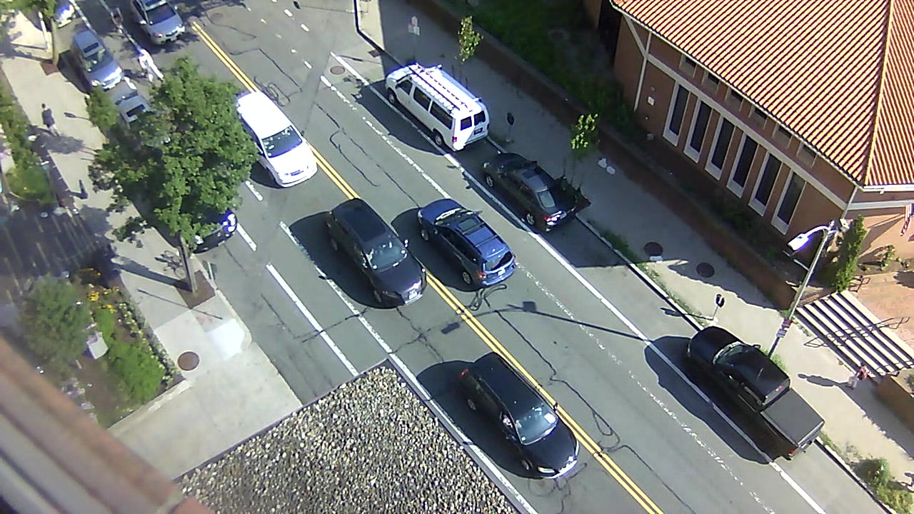
Figure 1: A normal frame from the Street Scene dataset.

After working on this problem, we think there are deficiencies in existing datasets for the single scene formulation of video anomaly detection. These deficiencies include the simplicity of the scenes for many datasets, the small number of anomalous events, the lack of variety in anomalous events, the very low resolution of some datasets, existence of staged anomalies in some cases, inconsistency in annotation, and the lack of spatial ground truth (in addition to temporal) in some cases. Furthermore, the evaluation criteria that have become standard practice for video anomaly detection have problems. Namely, the criteria do not properly evaluate spatial localization and do not properly count false positives. In short, they do not give a realistic picture of how an algorithm will perform in practice.

The goal of this paper is to shift the focus of video anomaly detection research to more realistic datasets and more useful evaluation criteria. We introduce a new dataset for video anomaly detection, called Street Scene, that has more labeled anomalous events and a greater variety of anomalies than previous datasets for single scene anomaly detection. Street Scene contains video of a two-way urban street including bike lanes and pedestrian sidewalks (see Figure 1). The video is high resolution and captures a scene with a large variety of activity. We also suggest two new evaluation criteria which we believe give a more accurate picture of how video anomaly detection algorithms will perform in practice than the existing criteria. Finally, we present two variations of a novel algorithm which outperform two state-of-the-art algorithms on Street Scene and set a more realistic baseline for future work to compare against.

2 Existing Datasets and Evaluation Criteria

There are a handful of publicly available datasets used to evaluate video anomaly detection algorithms. We discuss each of these below and summarize them in Table 1.

Dataset	Total	Training	Testing	Anomalous	Anomaly	Ground	Resolution
	Frames	Frames	Frames	Events	Types	Truth
UCSD Ped1	14,000	6800	7200	54	5	Spatial, Temporal	238 x 158
UCSD Ped2	4560	2550	2010	23	5	Spatial, Temporal	360 x 240
Subway entrance∗	86,535	18,000	68,535	66	5	Temporal	512 x 384
Subway exit∗	38,940	4,500	34,440	19	3	Temporal	512 x 384
CUHK Avenue	30,652	15,328	15,324	47	5	Spatial, Temporal	640 x 360
UMN∗∗	3,855	N/A	N/A	11	1	Temporal	320 x 240
Street Scene	203,257	56,847	146,410	205	17	Spatial, Temporal	1280 x 720

Table 1: Characteristics of video anomaly detection datasets for the single scene formulation. ^∗using 15fps ^∗∗aggregates from 3 cameras.

UCSD Pedestrian: The most widely used video anomaly detection dataset is the UCSD pedestrian anomaly dataset [18] which consists of two separate datasets containing video from two different static cameras (labeled Ped1 and Ped2), each looking at a pedestrian walkway. The test videos contain 5 different types of anomalies: “bike”, “skater”, “cart”, “walk across”, and “other”.

Despite being widely used, this dataset has various deficiencies. One is that it is modest in size, in terms of number of frames, total anomalies, and number of different types of anomalies. Another is that all of the anomalies can be detected by only analyzing a single frame at a time.

Subway: The Subway dataset [2] contains two long videos of a subway entrance and exit that mainly capture people entering and leaving through turnstiles. It is also actually two separate datasets. Anomalous activities include people jumping or squeezing around the turnstiles, walking the wrong direction, and a person cleaning the walls. Because only two long videos are provided, there are various ambiguities with this dataset such as what frame rate to extract frames, which frames to use as train/test and exactly which frames are labeled as anomalous. Also, there is no spatial ground truth provided.

CUHK Avenue: Another widely used dataset is called CUHK Avenue [22]. This dataset consists of short video clips taken from a single outdoor surveillance camera looking at the side of a building with a pedestrian walkway in front of it. The main activity consists of people walking and going into or out of the building. Anomalies are mostly staged and consist of actions such as a person throwing papers or a backpack into the air, or a child skipping across the walkway. Like UCSD, this dataset also has a small number and variety of anomalies.

UMN: The UMN dataset contains 11 short clips of 3 scenes of people meandering around an outdoor field, an outdoor courtyard, or an indoor foyer. In each of the clips the anomaly consists of all of the people suddenly running away, hinting at a frantic evacuation scenario. The scene is staged and there is one anomalous event per clip. There is no clear specification of a split between training and testing frames and anomalies are only labeled temporally.

Other Datasets: There are two other datasets that should be mentioned although they do not fall under the single scene formulation of video anomaly detection. One is the ShanghaiTech dataset introduced in a paper by Liu et al. [20]. It consists of 13 different scenes each with multiple training and testing sequences. The dataset is intended to be used to learn a single model and thus does not follow the single scene formulation. While it is conceivable to treat it as 13 separate datasets, this is problematic since many of the videos for a particular scene have significant changes in viewpoint and some have very little training video. Furthermore, treating it as separate datasets would yield an average of 10 anomalous events per scene which is very small.

Another dataset from Sultani et al. [36] (the UCF-Crime dataset) contains a large set of internet videos taken from hundreds of different cameras. This dataset is intended for a very different formulation of video anomaly detection more akin to activity detection. In their formulation, both anomalous and normal video is given for training. The dataset consists of videos from many scenes labeled with predefined anomalous activities as well as video with only ”normal” activities. For testing, only temporal labels are available, meaning spatial evaluation cannot be done. While this dataset is interesting, it is for a very different version of the problem and is not applicable to the single scene version that we are concerned with here.

General video surveillance/recognition datasets such as [19, 41, 26, 27] have not been used to evaluate video anomaly detection since they are not specifically curated for this purpose and do not contain sufficient ground truth annotations.

2.1 Evaluation Criteria

Almost every recent paper for video anomaly detection [24, 25, 38, 16, 33, 30, 6, 23, 39, 37, 40, 10, 7, 34, 22, 31, 20, 3, 4, 11, 12, 21, 29, 28, 35, 32, 14, 13] has used one or both of the evaluation criteria specified in Li et al. [18] which also introduced the UCSD pedestrian dataset. The first criterion, referred to as the frame-level criterion, counts a frame with any detected anomalous pixels as a positive frame and all other frames as negative. The frame-level ground truth annotations are then used to determine which detected frames are true positives and which are false positives, thus yielding frame-level true positive and false positive rates. This criterion uses no spatial localization and counts a frame as a correct detection (true positive) even if the detected anomalous pixels do not overlap with any ground truth anomalous pixels. Even the authors who proposed this criterion stated that they did not think it was the best one to use [18]. We have observed that some methods that claim state-of-the-art performance on frame-level criterion perform poor spatial localization in practice.

The other criterion is the pixel-level criterion and tries to take into account the spatial locations of anomalies. Unfortunately, it does so in a problematic way. The pixel-level criterion still counts true and false positive frames as opposed to true and false positive anomalous regions. A frame with ground truth anomalies is counted as a true positive detection if at least 40% of the ground truth anomalous pixels are detected. Other pixels detected as anomalous that do not overlap with ground truth are ignored. Any frame with no ground truth anomalies is counted as a false positive frame if at least one pixel is detected as anomalous. Given these rules, a simple post-processing of the anomaly score maps makes the pixel-level criterion equivalent to the frame-level criterion. The post-processing is: for any frame with at least one detected anomalous pixel, label every pixel in that frame as anomalous. This would guarantee a correct detection if the frame has a ground truth anomaly (since all of the ground truth anomalous pixels are covered) and would not further increase the false positive rate if it does not (since one or more detected pixels on a frame with no anomalies counts as a single false positive). This makes it clear that the pixel-level criterion does not reward tightness of localization or penalize looseness of it nor does it properly count false positives since false positive regions are not even counted for frames containing ground truth anomalies, and a frame with no ground truth anomaly can only have a single false positive even if an algorithm falsely detects many different false positive regions in that frame.

Better evaluation criteria are clearly needed.

3 Description of Street Scene

Anomaly Class	Instances	Anomaly Class	Instances	Anomaly Class	Instances
1. Jaywalking	61	7. Biker on sidewalk	7	13. Skateboarder in bike lane	2
2. Biker outside lane	42	8. Pedestrian reverses direction	6	14. Person sitting on bench	2
3. Loitering	36	9. Car u-turn	5	15. Metermaid ticketing car	1
4. Dog on sidewalk	11	10. Car illegally parked	5	16. Car turning from parking space	1
5. Car outside lane	10	11. Person opening trunk	4	17. Motorcycle drives onto sidewalk	1
6. Worker in bushes	8	12. Person exits car on street	3

Table 2: Meta-data of anomaly classes and number of instances of each in the Street Scene dataset.

To address the deficiencies of existing datasets, we introduce the Street Scene dataset. Street Scene consists of 46 training video sequences and 35 testing video sequences taken from a static USB camera looking down on a scene of a two-lane street with bike lanes and pedestrian sidewalks. See Figure 1 for a typical frame from the dataset. Videos were collected from the camera at various times during two consecutive summers. All of the videos were taken during the daytime. The dataset is challenging because of the variety of activity taking place such as cars driving, turning, stopping and parking; pedestrians walking, jogging and pushing strollers; and bikers riding in bike lanes. In addition the videos contain changing shadows, and moving background such as a flag and trees blowing in the wind. There are a total of 203,257 color video frames (56,847 for training and 146,410 for testing) each of size 1280 x 720 pixels. The frames were extracted from the original videos at 15 frames per second.

We wanted the dataset to contain only “natural” anomalies, i.e. not staged by “actors”. To this end, the training sequences were chosen to meet the following conditions:

(1) If people are present, they are walking, jogging or pushing a stroller in one direction on a sidewalk; or they are getting into or out of their car including walking alongside their car; or they are stopped in front of a parking meter.

(2) If a car is present, it is legally parked; or it is driving in the appropriate direction in a car lane; or stopped in a car lane due to traffic; or making a legal turn across traffic; or leaving/entering a parking spot on the side of the street.

(3) If bikers are present, they are riding in the correct direction in a bike lane; or turning from an intersecting road into a bike lane or from a bike lane onto an intersecting road.

These conditions for normal activity imply that the following activities, for example, are anomalous and thus do not appear in the training videos: Pedestrians jaywalking across the road, pedestrians loitering on the sidewalk, pedestrians walking one direction and then turning around and walking the opposite direction, bikers on the sidewalk, bikers outside a bike lane (except when turning into a bike lane from the intersecting street) cars making u-turns, cars parked illegally, cars outside a car lane (except when turning or parked, parking or leaving a parking spot).

The 35 testing sequences have a total of 205 anomalous events consisting of 17 different anomaly types. A complete list of anomaly types and the number of each in the test set is given in Table 2, for descriptive purposes only.

The Street Scene dataset can be downloaded from http://www.merl.com/demos/video-anomaly-detection. Ground truth annotations are provided for each testing video in the form of bounding boxes around each anomalous event in each frame. Each bounding box is also labeled with a track number, meaning each anomalous event is labeled as a track of bounding boxes. A single frame can have more than one anomaly labeled.

4 New Evaluation Criteria

As discussed in Section 2.1, the main criteria used by previous work to evaluate video anomaly detection accuracy have significant problems. Sabokrou et al. [32] also recognized the problems with the standard criteria and proposed the Dual Pixel Level criteria. While this is an improvement, it still cannot correctly count true positives and false positives in frames with (a) multiple anomalies, (b) both true positive as well as false positive detections and (c) multiple false positive detections. A good evaluation criterion should measure the fraction of anomalies an algorithm can detect and the number of false positive regions an algorithm can be expected to mistakenly find per frame.

Our new evaluation criteria are informed by the following considerations. Similar to object detection criteria, using the intersection over union (IOU) between a ground truth anomalous region and a detected anomalous region for determining whether an anomaly is detected is a good way to insure rough spatial localization. For video anomaly detection, the IOU threshold should be low to allow some imprecision in localization because of issues like imprecise labeling (bounding boxes) and the fact that some algorithms detect anomalies that are close to each other as one large anomalous region which should not be penalized. Similarly, shadows may cause larger anomalous regions than what are labeled. We do not think such larger than expected anomalous-region detections should be penalized. We use an IOU threshold of 0.1 in our experiments.

Also, because a single frame can have multiple ground-truth anomalous regions, correct detections should be counted at the level of anomalous regions, not frames.

False positives should be counted for each falsely detected anomalous region, i.e. by each detected anomalous region that does not significantly overlap with a ground truth anomalous region. This allows more than one false positive per frame and also false positives in frames with ground truth annotations, unlike the previous criteria.

In practice, for an anomaly that occurs over many frames, it is important to detect the anomalous region in at least some of the frames, but it is usually not important to detect the region in every frame in the track. This is especially true considering the ambiguities for when to begin and end an anomalous track mentioned earlier, and in cases where anomalous activity is severely occluded for a few frames. Because the Street Scene dataset provides track numbers for each anomalous region which uniquely identify the event to which an anomalous region belongs, it is easy to compute such a criterion. The new criteria resulting from these considerations are similar to evaluation criteria used in object detection and object tracking [9, 8] but similar criteria have not been used for video anomaly detection in the past.

4.1 Track-Based Detection Criterion

The track-based detection criterion measures the track-based detection rate (TBDR) versus the number of false positive regions per frame.

A ground truth track is considered detected if at least a fraction $\alpha$ of the ground truth regions in the track are detected.

A ground truth region in a frame is considered detected if the intersection over union (IOU) between the ground truth region and a detected region is greater than or equal to $\beta$.

$$\vspace{-6pt}\mbox{TBDR}=\frac{\mbox{num. of anomalous tracks detected}}{\mbox{total num. of anomalous tracks}}.$$ (1)

A detected region in a frame is a false positive if the IOU between it and every ground truth region in that frame is less than $\beta$.

$$\vspace{-6pt}\mbox{FPR}=\frac{\mbox{total false positive regions}}{\mbox{total frames}}$$ (2)

where FPR is the false-positive rate per frame.

Note that a single detected region can cover two or more different ground truth regions so that each ground truth region is detected (although this is rare).

In our experiments below, we use $\alpha=0.1$ and $\beta=0.1$.

4.2 Region-Based Detection Criterion

The region-based detection criterion measures the region-based detection rate (RBDR) over all frames in the test set versus the number of false positive regions per frame.

As with the track-based detection criterion, a ground truth region in a frame is considered detected if the intersection over union (IOU) between the ground truth region and a detected region is greater than or equal to $\beta$.

$$\vspace{-6pt}\mbox{RBDR}=\frac{\mbox{num. of anomalous regions detected}}{\mbox{total num. of anomalous regions}}.$$ (3)

The RBDR is computed over all ground truth anomalous regions in all frames of the test set.

The number of false positives per frame is calculated in the same way as with the track-based detection criterion.

As with any detection criterion, there is a trade-off between detection rate (true positive rate) and false positive rate which can be captured in a ROC curve computed by changing the threshold on the anomaly score that determines which regions are detected as anomalous.

When a single number is desired, we suggest summarizing the performance with the average detection rate for false positive rates from 0 to 1, i.e. the area under the ROC curve for false positive rates less than or equal to 1.

5 Baseline Algorithms

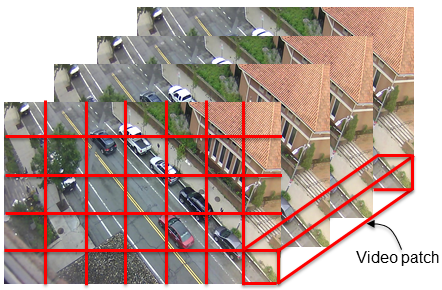
Figure 2: Illustration of a grid of regions partitioning a video frame and a video patch encompassing 4 frames. This figure show non-overlapping regions, but in our experiments we use overlapping regions.

We describe two variations of a novel algorithm for video anomaly detection which we evaluate along with two previously published algorithms on the Street Scene dataset in Section 6. The new algorithm is based on dividing the video into spatio-temporal regions which we call video patches, storing a set of exemplars to represent the variety of video patches occuring in each region, and then using the distance from a testing video patch to the nearest neighbor exemplar as the anomaly score. As with previous work such as [14, 22], our baseline algorithm uses video patches (also called spatio-temporal cubes) as the basic building block, but differs in the features and type of model we use.

First, each video is divided into a grid of spatio-temporal regions of size $H\times W\times T$ pixels with spatial step size $s$ and temporal step size 1 frame. In the experiments in Section 6 we choose $H$=40 pixels, $W$=40 pixels, T=4 or 7 frames, and $s$ = 20 pixels. See Figure 2 for an illustration.

The baseline algorithm has two phases: a training or model-building phase and a testing or anomaly detection phase. In the model-building phase, the training (normal) videos are used to find a set of video patches (represented by feature vectors described later) for each spatial region that represent the variety of activity in that spatial region. We call these representative video patches, exemplars. In the anomaly detection phase, the testing video is split into the same regions used in training and for each testing video patch, the nearest exemplar from its spatial region is found. The distance to the nearest exemplar is the anomaly score.

The only differences between the two variations are the feature vector used to represent each video patch and the distance function used to compare two feature vectors.

The foreground (FG) mask variation uses blurred FG masks for each frame in a video patch. The FG masks are computed using a background (BG) model that is updated as the video is processed. The BG model used in the experiments is a very simple mean color value per pixel although a more sophisticated model could be easily substituted.

The FG mask is then blurred using a Gaussian kernel to make the $L_{2}$ distance between FG masks more robust. The FG mask feature vector is formed by concatenating all of the blurred FG masks from all frames in a video patch and then vectorizing (see Figure 3).

The flow-based variation uses optical flow fields computed between consecutive frames in place of FG masks. The flow fields within the region of each video patch frame are concatenated and then vectorized to yield a feature vector twice the length of the feature vector from the FG mask baseline (due to the dx and dy components of the flow field). In our experiments we use the optical flow algorithm of Kroeger et al. [17] to compute flow fields.

In the model building phase, a distinct set of exemplars is selected to represent normal activity in each spatial region. Our exemplar selection method is straightforward. For a particular spatial region, the exemplar set is initialized to the empty set. We slide a spatial-temporal window (with step size equal to one frame) along the temporal dimension of each training video to give a series of video patches which we represent by either a FG-mask based feature vector or a flow-based feature vector depending on the algorithm variation as described above. For each video patch, we compare it to the current set of exemplars. If the distance to the nearest exemplar is less than a threshold then we discard that video patch. Otherwise we add it to the set of exemplars.

The distance function used to compare two exemplars depends on the feature vector. For blurred FG mask feature vectors, we use $L_{2}$ distance. For flow-field feature vectors we use normalized $L_{1}$ distance:

$$dist({\bf u},{\bf v})=\sum_{i}\frac{|u_{i}-v_{i}|}{|u_{i}|+|v_{i}|+\epsilon}$$ (4)

where $u$ and $v$ are two flow-based feature vectors and $\epsilon$ is a small positive constant used to avoid division by zero.

Given a model of normal video which consists of a different set of exemplars for each spatial region of the video, the anomaly detection is simply a series of nearest neighbor lookups. For each spatial region in a sequence of $T$ frames of a testing video, compute the feature vector representing the video patch and then find the nearest neighbor in that region’s exemplar set. The distance to the closest exemplar is the anomaly score for that video patch.

This yields an anomaly score per overlapping video patch. These are used to create a per-pixel anomaly score matrix for each frame. The anomaly score for a video patch is stored in the middle frame for that set of $T$ frames. The first $T/2-1$ frames and the last $T/2+1$ frames of the testing video are not assigned any anomaly scores from video patches and thus get all 0’s. A pixel covered by two or more video patches is assigned the average score from all video patches that include the pixel.

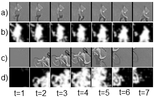
Figure 3: Example blurred FG masks, concatenated and vectorized into a feature vector. a and c show two video patches consisting of 7 frames cropped around a spatial region. b and d show the corresponding blurred FG masks.

When computing ROC curves according to either of the track-based or region-based criteria, for a given threshold, all pixels with anomaly scores above the threshold are labeled anomalous. Then anomalous regions are found by computing the connected components of anomalous pixels. These anomalous regions are compared to the ground truth regions according to one of the above criteria.

6 Experiments

In addition to the two variations of our baseline video anomaly detection method, we also tested two previously published methods. The first is the dictionary method of Lu et al. [22] which fits a sparse combination of dictionary basis feature vectors to a feature vector representing each spatio-temporal window of the test video. A dictionary of basis feature vectors is learned from the normal training videos for each spatial region independently. This method reported good results on UCSD, Subway and CUHK Avenue datasets. Code was provided by the authors.

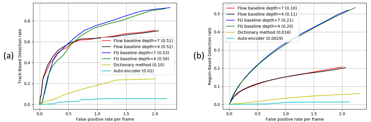
Figure 4: Track-based (a) and region-based (b) ROC curves for different methods on Street Scene

Figure 5: Frame-level (a) and pixel-level (b) ROC curves for different methods on Street Scene

The second method is from Hasan et al. [10] which uses a deep network auto-encoder to learn a model of normal frames. The anomaly score for each pixel is the reconstruction error incurred by passing a clip containing the pixel through the auto-encoder. This assumes that anomalous regions of a frame will not be well reconstucted. This method is also competitive with other state-of-the-art results on standard datasets and evaluation criteria. We used our own implementation of this method.

We have been unable to find code available for other algorithms, but hope that researchers will report the results of their algorithms on Street Scene in the near future.

Figures 4 (a) and (b) show ROC curves for our baseline methods as well as the dictionary and auto-encoder methods on Street Scene using the newly proposed track-based and region-based criteria. The numbers in parentheses for each method in the figure legends are the areas under the curve for false positive rates from 0 to 1. Clearly, the dictionary and auto-encoder methods perform poorly on Street Scene. Our baseline methods do much better although there is still much room for improvement.

While the dictionary method works well on other, smaller datasets, the sparse dictionary model does not seem to be expressive enough to reconstruct many normal testing video patches on the larger and more varied Street Scene.

The auto-encoder method tries to model whole frames at once as opposed to creating smaller models for different spatial regions. While this seems to work on previous datasets, it does not seem to work with the huge variety of normal variations present in Street Scene.

Our baseline algorithms perform reasonably well on Street Scene. They store a large set of exemplars (typically between 1000 and 3000 exemplars) in regions where there is a lot of activity such as the street, sidewalk and bike lane regions. On other regions such as the building walls or roof tops, only a single exemplar is stored.

For the two baseline variations using the track-based criteria, the flow-based method does best for low false-positive rates (arguably the most important part of the ROC curve). The flow field provides more useful information than FG masks for most of the anomalies (the main exception being loitering anomalies which are discussed below). The FG-based method does better using the region-based criterion. The number of frames used in a video patch (4 or 7) does not have a large effect on either variation.

The baseline algorithms do best at detecting anomalous activities such as jaywalking, illegal u-turn, and bikers or cars outside their lanes because these anomalies have distinctive motions compared to the typical motions in the regions where they occur.

The loitering anomalies (and other largely static anomalies such as illegally parked cars) are the most difficult for the baseline methods because they do not contain any motion except at the beginning in which a walking person transitions to loitering. For the flow-based method, the loitering anomalies are completely invisible. For the FG-based method, the beginning of the loitering anomaly is visible since the BG model takes a few frames to absorb the motionless person. This is the main reason why the flow-based method is worse than the FG-based method for higher detection rates. The FG-based method can detect some of the loitering anomalies while the flow-based method cannot.

A similar effect explains the region-based results in which the FG-based method does better than the flow-based method. The loitering and other “static” anomalies make up a disproportionate fraction of the total anomalous regions because many of them occur over many frames. The FG-based method detects some of these regions while the flow-based method misses essentially all of them. So even though the flow-based method detects a greater fraction of all anomalous tracks (at low false positive rates) it detects a smaller fraction of all anomalous regions.

Some visualizations of the detection results for the flow-based method (using T=4) are shown in Figures 6 and 7. In the figures, red tinted pixels are anomaly detections and blue boxes show the ground truth annotations. Figure 6 shows the correct detection of a motorcycle that rides onto a sidewalk. Figure 7 shows a detected jaywalker as well as a false positive region.

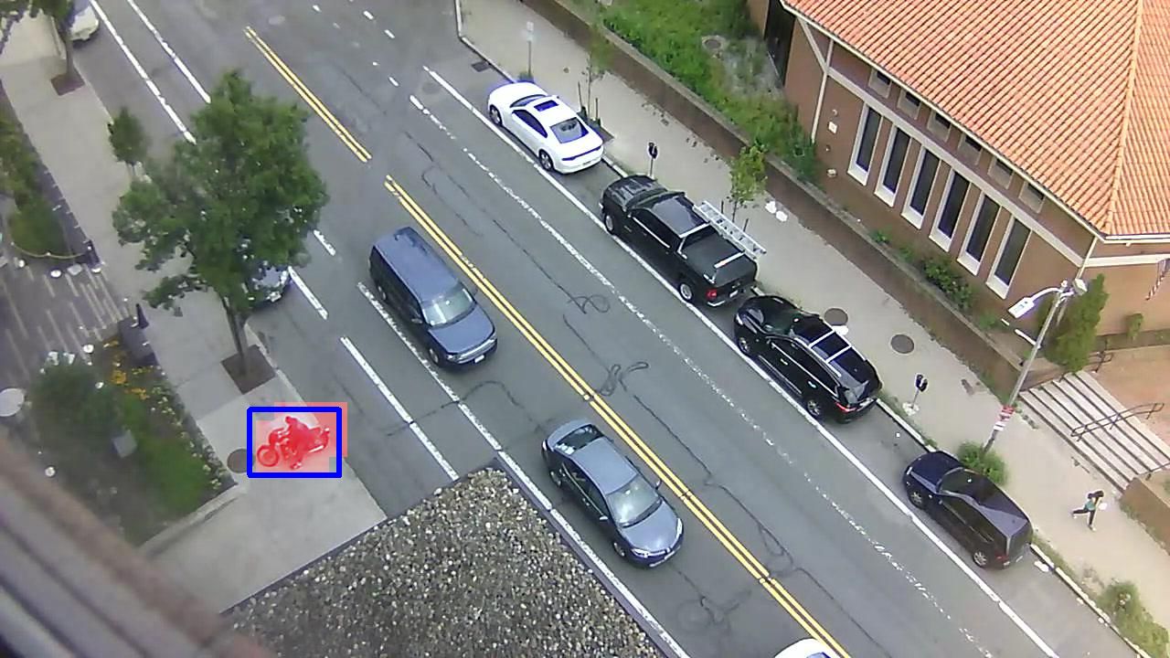
Figure 6: Detection result for flow baseline showing correctly detected motorcycle driving onto the sidewalk.

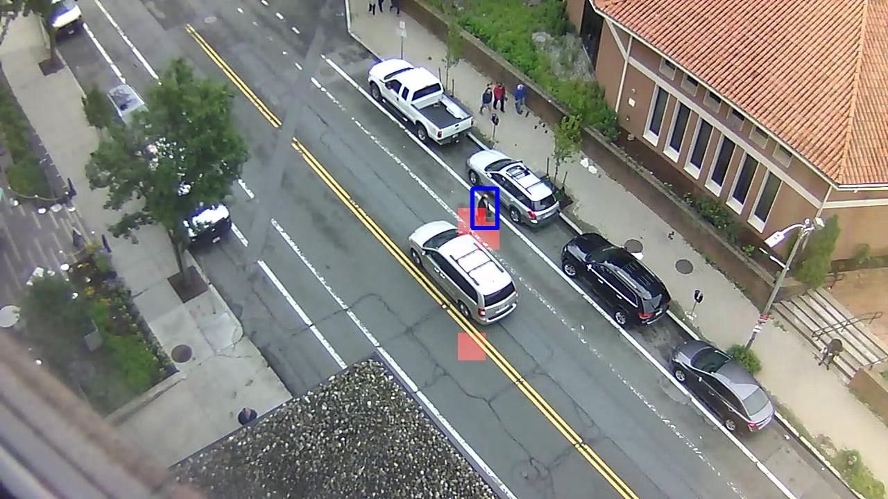
Figure 7: Detection result for flow baseline that is counted as missed detection but no false positive by pixel-level criterion and is counted as one correct detection and one false positive by the track-based and region-based criteria.

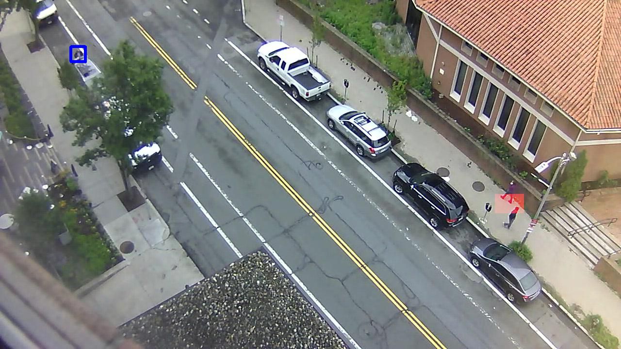
Figure 8: Detection result for flow baseline showing missed detection and false positive region that is counted as correct detection with no false positives by frame-level criterion.

We also show results for the two baseline algorithms as well as the dictionary and auto-encoder methods using the traditional frame-level and pixel-level criteria in Figures 5 (a) and (b). We show the results for the purpose of illustrating the deficiencies of these criteria, but not for comparison with future work. We do not think these criteria should be used for Street Scene going forward. The frame-level results (which do not take spatial localization into account) suggest that the auto-encoder method does about as well as the foreground baseline and the dictionary method is almost as good as the flow baseline. However, when we look at what regions of each frame the auto-encoder and dictionary methods actually detect as anomalous, the accuracy is quite poor. This can be seen in the track-based, region-based and pixel-level ROC curves as well as by visual inspection. Figure 8 shows the output of the flow baseline for a frame that contains a “person opening trunk” anomaly in the top, left. The frame-level criterion counts this frame as a correct detection even though the detected pixels are nowhere near the ground truth anomaly but are in fact a false positive. The pixel-level ROC curves in Figure 5 (b) are more reasonable and in better agreement with the track-based and region-based ROC curves, but as mentioned earlier this criteria has the serious flaw that a very simple post-processing of anomaly scores would boost these curves so they are exactly the same as the frame-level ROC curves. Figure 7 shows an example of a jaywalk anomaly that has fewer than 40% of its pixels detected and is therefore a missed detection according to the pixel-level criterion. This criteria also ignores a false-positive region below the car. The region and track-based criterion would count this as a correct detection and one false positive. We argue that this is a better fit to human intuition about how this frame should be counted.

7 Conclusions

We have presented a new large-scale dataset and new evaluation criteria for video anomaly detection that we hope will help to spur new innovations in this field. The Street Scene dataset is a more complex scene and has almost as many anomalous events as all currently available datasets combined. The new evaluation criteria fix the problems with the criteria typically used in this field, and will give a more realistic idea of how well an algorithm performs in practice.

In addition, we have presented two variations of a new video anomaly detection algorithm as a baseline for future work to compare against; they are straightforward and outperform two previously published algorithms which do well on previous datasets but not on Street Scene. The new nearest-neighbor based algorithms may form an interesting foundation to build on.

Acknowledgement: Thanks to Raju Vatsavai and Zexi Chen of NC State for help with reimplementing [10].

8 Supplemental Material

8.1 More Detection Result Visualizations

We show more examples of our detection results using our flow-based algorithm with $T=4$ frames in Figures 9 through 17. In each of the frames shown, the red tinted pixels are detected as anomalous by our algorithm. The blue rectangles show the ground truth annotations in each frame.

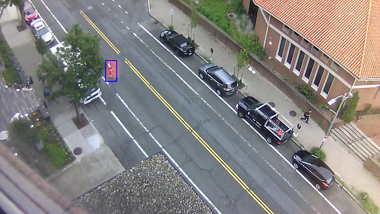
Figure 9: Detection result for flow-based method showing correctly detected biker outside of the bike lane.

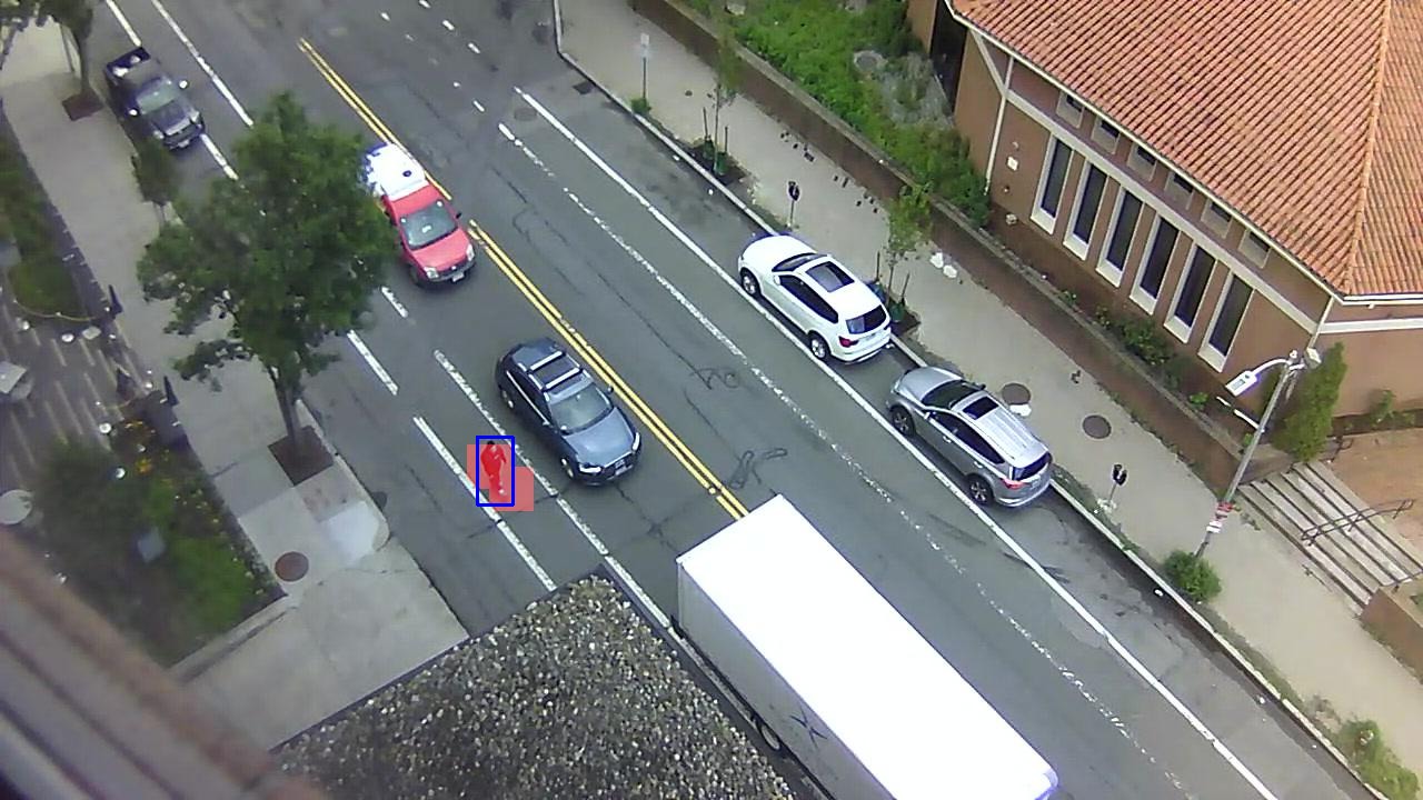
Figure 10: Detection result for flow-based method showing correctly detected skateboarder in a bike lane.

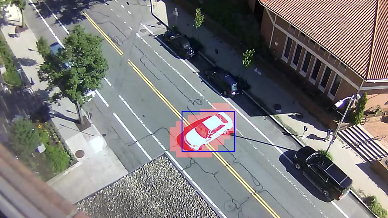
Figure 11: Detection result for flow-based method showing correctly detected car u-turn.

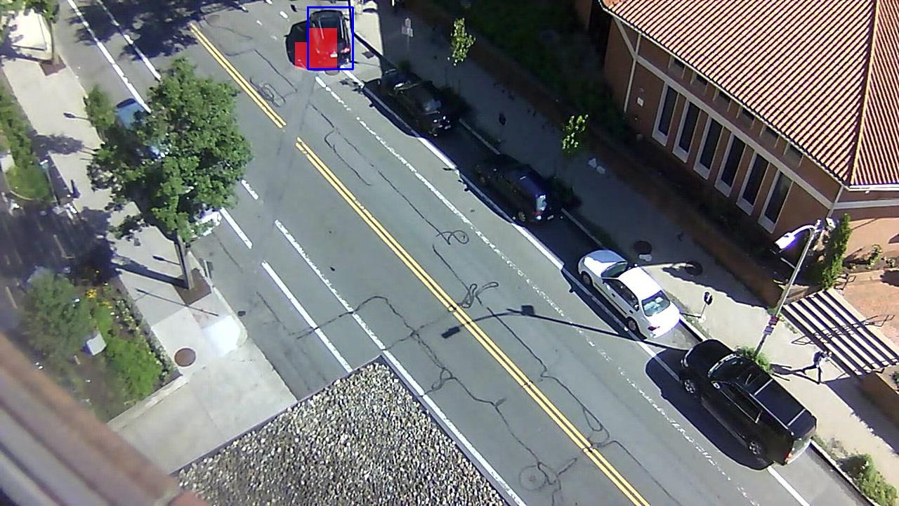
Figure 12: Detection result for flow-based method showing correctly detected illegal parking.

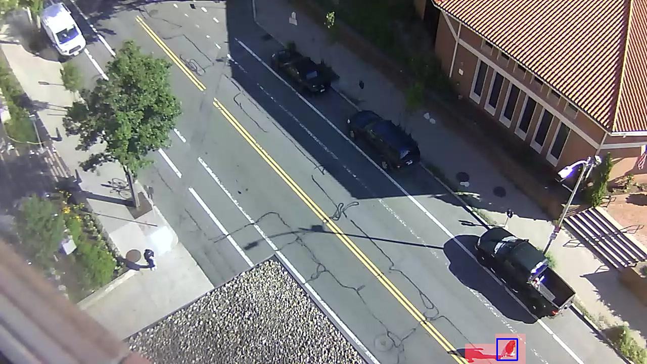
Figure 13: Detection result for flow-based method showing correctly detected jaywalker.

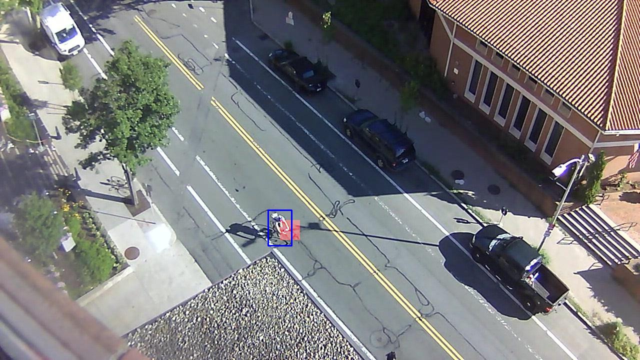
Figure 14: Detection result for flow-based method showing correctly detected biker outside of the bike lane.

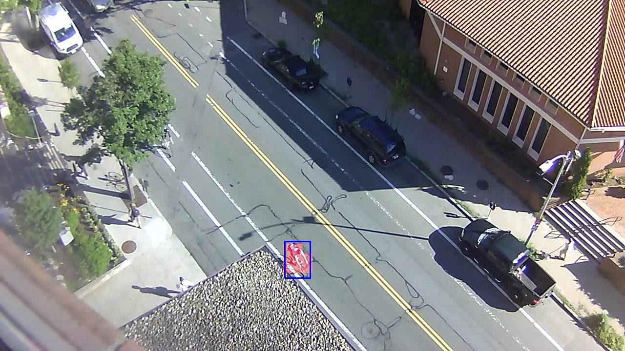
Figure 15: Detection result for flow-based method showing correctly detected biker outside of the bike lane.

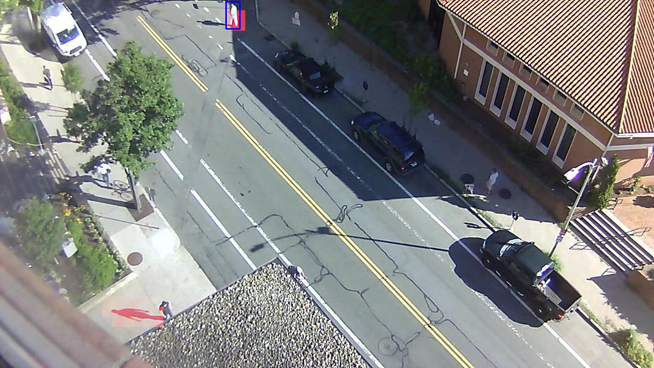
Figure 16: Detection result for flow-based method showing correctly detected jaywalker as well as a false positive.

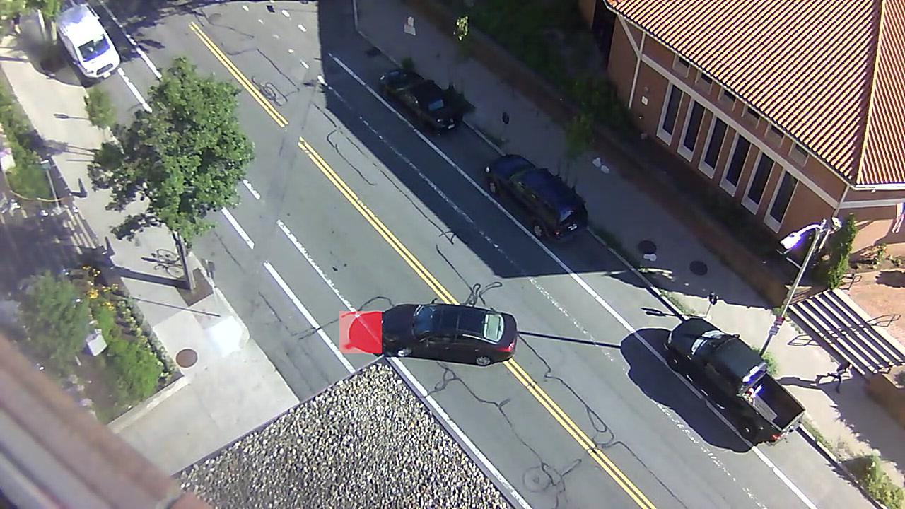
Figure 17: Detection result for flow-based method showing a false positive caused by a shadow of a car.

8.2 Results of baseline algorithms on UCSD Ped1 and Ped2

The baseline video anomaly detection method described in the paper is not the focus of this paper and is not claimed to be superior to the current state of the art on existing datasets. The purpose is to provide reasonable baseline results on Street Scene for future work to compare against since the available implementations of previous algorithms do not perform well on Street Scene. However, readers may be interested in how our exemplar-based algorithm performs on existing datasets. Table 3 shows results for our foreground baseline algorithm on UCSD Ped1 and Ped2 datasets using the traditional frame-level and pixel-level criteria. We also show results from other recent papers for comparison. Our results are comparable to many recent results especially using the pixel-level criterion.

Method	Ped1 Frame-level		Ped1 Pixel-level		Ped2 Frame-level		Ped2 Pixel-level
	AUC	EER	AUC	EER	AUC	EER	AUC	EER
Dictionary method [22]	91.8%	15%	63.8%	43%	-	-	-	-
Autoencoder [10]	81.0%	27.9%	-	-	90.0%	21.7%	-	-
AMDN [40]	92.1%	16%	67.2%	40.1%	90.8%	17%	-	-
MDT [18]	81.8%	25%	44.1%	58.0%	85.0%	25%	44.0%	-
Video parsing [3]	91.0%	18%	83.6%	23%	92.0%	14%	-	-
ST Video parsing [4]	93.9%	12.9%	84.2%	20.5%	94.6%	10.6%	81.1%	11.2
Plug and play CNN [28]	95.7%	8%	64.5%	-%	88.4%	18%	-	-
Our FG Baseline	77.3%	25.9%	69.3%	39.4%	88.3%	18.9%	83.9%	23.5%

Table 3: Traditional frame-level and pixel-level results on UCSD Ped1 and Ped2.

9 Detailed List of Anomalies in Street Scene

Tables 4 and 5 list every annotated anomaly in the Street Scene dataset for all 35 testing videos. This list will be included with the dataset when it is publicly released (along with the ground truth bounding boxes for all frames). The lists give a good sense of what is contained in the data set. It is purely for informative purposes. The anomaly types are not used in the evaluation criteria.

Test	Anomaly	Anomaly Type	Test	Anomaly	Anomaly Type	Test	Anomaly	Anomaly Type
video	Index		video	Index		video	Index
Test001	1	Jaywalk	Test009	1	Biker outside lane	Test015	4	Biker outside lane
	2	Worker in bushes		2	Biker outside lane		5	Jaywalk
Test002	1	Person opening trunk		3	Biker on sidewalk		6	Biker outside lane
	2	Loitering	Test010	1	Car u-turn		7	Biker outside lane
	3	Loitering		2	Car Illegally parked		8	Biker outside lane
	4	Loitering		3	Jaywalk		9	Biker outside lane
	5	Jaywalk		4	Biker outside lane	Test016	1	Jaywalk
	6	Jaywalk		5	Jaywalk		2	Biker outside lane
	7	Jaywalk		6	Jaywalk		3	Biker outside lane
Test003	1	Jaywalk	Test011	1	Loitering	Test017	1	Dog
	2	Jaywalk		2	Car u-turn		2	Loitering
	3	Jaywalk		3	Biker outside lane		3	Loitering
Test004	1	Car u-turn		4	Biker outside lane		4	Jaywalk
	2	Jaywalk		5	Biker outside lane		5	Jaywalk
	3	Car outside lane		6	Jaywalk		6	Jaywalk
	4	Jaywalk		7	Car illegally parked		7	Pedestrian reverses direction
	5	Jaywalk		8	Jaywalk		8	Loitering
Test005	1	Loitering		9	Biker outside lane		9	Jaywalk
	2	Dog		10	Jaywalk		10	Loitering
	3	Loitering	Test012	1	Loitering		11	Dog
	4	Loitering		2	Loitering		12	Loitering
	5	Jaywalk		3	Car u-turn		13	Biker outside lane
	6	Loitering		4	Biker outside lane	Test018	1	Biker outside lane
	7	Loitering		5	Loitering		2	Biker outside lane
	8	Jaywalk		6	Dog		3	Biker outside lane
	9	Jaywalk	Test013	1	Dog		4	Pedestrian reverses direction
	10	Loitering		2	Loitering		5	Loitering
	11	Loitering		3	Biker on sidewalk		6	Biker outside lane
	12	Loitering		4	Dog		7	Biker outside lane
	13	Loitering		5	Loitering		8	Loitering
	14	Jaywalk		6	Dog		9	Metermaid ticketing car
Test006	1	Person sitting on bench		7	Loitering		10	Pedestrian reverses direction
	2	Person opening trunk		8	Loitering		11	Loitering
	3	Jaywalk		9	Dog		12	Biker on sidewalk
Test007	1	Jaywalk		10	Loitering	Test019	1	Person exits car on street
	2	Skateboarder in bike lane		11	Person opening trunk	Test020	1	Jaywalk
	3	Skateboarder in bike lane	Test014	1	Jaywalk		2	Jaywalk
	4	Biker on sidewalk	Test015	1	Car turning from parking space		3	Jaywalk
Test008	1	Jaywalk		2	Biker outside lane	Test021	1	Jaywalk
	2	Jaywalk		3	Biker outside lane		2	Biker outside lane

Table 4: List of anomalies labeled in each testing video

Test	Anomaly	Anomaly Type	Test	Anomaly	Anomaly Type	Test	Anomaly	Anomaly Type
video	Index		video	Index		video	Index
Test021	3	Dog	Test025	4	Biker outside lane	Test029	11	Car outside lane
	4	Biker outside lane		5	Biker outside lane	Test030	1	Car outside lane
	5	Biker outside lane		6	Biker outside lane		2	Pedestrian reverses direction
	6	Jaywalk		7	Biker on sidewalk		3	Car outside lane
	7	Loitering		8	Jaywalk	Test031	1	Person sitting on bench
Test022	1	Loitering	Test026	1	Biker outside lane		2	Biker outside lane
	2	Dog		2	Biker outside lane		3	Pedestrian reverses direction
	3	Loitering		3	Car outside lane		4	Jaywalk
	4	Loitering		4	Car outside lane		5	Motorcycle drives onto sidewalk
Test023	1	Dog		5	Loitering	Test032	1	Worker in bushes
	2	Biker outside lane		6	Biker on sidewalk		2	Worker in bushes
	3	Car u-turn	Test027	1	Jaywalk		3	Pedestrian reverses direction
	4	Biker on sidewalk		2	Jaywalk		4	Jaywalk
	5	Jaywalk		3	Jaywalk	Test033	1	Worker in bushes
	6	Biker outside lane		4	Jaywalk		2	Jaywalk
	7	Biker outside lane	Test028	1	Jaywalk		3	Jaywalk
	8	Biker outside lane		2	Biker outside lane	Test034	1	Worker in bushes
	9	Biker outside lane		3	Car outside lane		2	Jaywalk
	10	Biker outside lane	Test029	1	Illegal parking		3	Jaywalk
Test024	1	Jaywalk		2	Jaywalk		4	Worker in bushes
	2	Jaywalk		3	Jaywalk		5	Worker in bushes
	3	Jaywalk		4	Car illegally parked		6	Worker in bushes
	4	Jaywalk		5	Car outside lane	Test035	1	Jaywalk
	5	Jaywalk		6	Car outside lane		2	Jaywalk
	5	Biker outside lane		7	Car outside lane		3	Loitering
	6	Biker outside lane		8	Person exits car on street		4	Jaywalk
Test025	1	Biker on sidewalk		9	Person exits car on street		5	Loitering
	2	Jaywalk		10	Person opening trunk		6	Pedestrian reverses direction
	3	Jaywalk

Table 5: Continued list of anomalies labeled in each testing video

References

- [1] Unusual crowd activity dataset. http://mha.cs.umn.edu/Movies/Crowd-Activity-All.avi, 2008.
- [2] A. Adam, E. Rivlin, I. Shimshoni, and D. Reinitz. Robust real-time unusual event detection using multiple fixed-location monitors. IEEE Transactions on Pattern Analysis and Machine Intelligence (PAMI), 2008.
- [3] B. Antic and B. Ommer. Video parsing for abnormality detection. In IEEE International Conference on Computer Vision (ICCV), pages 2415–2422. IEEE, Nov. 2011.
- [4] B. Antic and B. Ommer. Spatio-temporal Video Parsing for Abnormality Detection. arXiv preprint arXiv:1502.06235, 2015.
- [5] Y. Benezeth, P.-M. Jodoin, V. Saligrama, and C. Rosenberger. Abnormal events detection based on spatio-temporal co-occurences. In IEEE Conference on Computer Vision and Pattern Recognition (CVPR), 2009.
- [6] K.-W. Cheng, Y.-T. Chen, and W.-H. Fang. Video anomaly detection and localization using hierarchical feature representation and gaussian process regression. In IEEE Conference on Computer Vision and Pattern Recognition (CVPR), pages 2909–2917, 2015.
- [7] Y. Cong, J. Yuan, and J. Liu. Abnormal event detection in crowded scenes using sparse representation. Pattern Recognition, 46(7):1851–1864, July 2013.
- [8] T. Ellis. Performance metrics and methods for tracking in surveillance. Third IEEE International Workshop on Performance Evaluation of Tracking and Surveillance, 01 2002.
- [9] M. Everingham, L. Van Gool, C. K. I. Williams, J. Winn, and A. Zisserman. The PASCAL Visual Object Classes Challenge 2012 (VOC2012) Results. http://www.pascal-network.org/challenges/VOC/voc2012/workshop/index.html.
- [10] M. Hasan, J. Choi, J. Neumann, A. Roy-Chowdhury, and L. Davis. Learning temporal regularity in video sequences. In IEEE Conference on Computer Vision and Pattern Recognition (CVPR), 2016.
- [11] R. Hinami, T. Mei, and S. Satoh. Joint detection and recounting of abnormal events by learning deep generic knowledge. In IEEE International Conference on Computer Vision (ICCV), 2017.
- [12] R. Ionescu, S. Smeureanu, B. Alexe, and M. Popescu. Unmasking the abnormal events in video. In IEEE International Conference on Computer Vision (ICCV), 2017.
- [13] R. T. Ionescu, F. S. Kahn, M.-I. Georgescu, and L. Shao. Object-centric auto-encoders and dummy anomalies for abnormal event detection in video. In IEEE Conference on Computer Vision and Pattern Recognition (CVPR), 2019.
- [14] R. T. Ionescu, S. Smeureanu, M. Popescu, and B. Alexe. Detecting abnormal events in video using narrowed normality clusters. In IEEE Winter Conference on Applications of Computer Vision (WACV), 2018.
- [15] J. Kim and K. Grauman. Observe locally, infer globally: a space-time mrf for detecting abnormal activities with incremental updates. In IEEE Conference on Computer Vision and Pattern Recognition (CVPR), 2009.
- [16] L. Kratz and K. Nishino. Anomaly detection in extremely crowded scenes using spatio-temporal motion pattern models. In IEEE Conference on Computer Vision and Pattern Recognition (CVPR), pages 1446–1453. IEEE, 2009.
- [17] T. Kroeger, R. Timofte, D. Dai, and L. V. Gool. Fast optical flow using dense inverse search. In European Conference on Computer Vision (ECCV), 2016.
- [18] W. Li, V. Mahadevan, and N. Vasconcelos. Anomaly detection and localization in crowded scenes. IEEE Transactions on Pattern Analysis and Machine Intelligence (PAMI), 2014.
- [19] K. Liu, L. Wu, H. Ma, W. Huang, and X. Dong. Generalized zero-shot learning for action recognition with web-scale video data. World Wide Web Internet and Web Information Systems, (7), 2017.
- [20] W. Liu, W. Luo, D. Lian, and S. Gao. Future frame prediction for anomaly detection - a new baseline. In IEEE Conference on Computer Vision and Pattern Recognition (CVPR), 2018.
- [21] Y. Liu, C. Li, and B. Poczos. Classifier two-sample test for video anomaly detections. In British Machine Vision Conference (BMVC), 2018.
- [22] C. Lu, J. Shi, and J. Jia. Abnormal event detection at 150 fps in matlab. In IEEE International Conference on Computer Vision (ICCV), 2013.
- [23] K. Ma, M. Doescher, and C. Bodden. Anomaly Detection In Crowded Scenes Using Dense Trajectories.
- [24] V. Mahadevan, W. Li, V. Bhalodia, and N. Vasconcelos. Anomaly detection in crowded scenes. In IEEE Confernce on Computer Vision and Pattern Recognition (CVPR), pages 1975–1981, June 2010.
- [25] R. Mehran, A. Oyama, and M. Shah. Abnormal crowd behavior detection using social force model. In IEEE Confernce on Computer Vision and Pattern Recognition (CVPR), pages 935–942. IEEE, 2009.
- [26] A.-T. Nghiem, F. Bremond, M. Thonnat, and V. Valentin. Etiseo, performance evaluation for video surveillance systems. In 2007 IEEE Conference on Advanced Video and Signal Based Surveillance, pages 476–481. IEEE, 2007.
- [27] S. Oh, A. Hoogs, A. Perera, N. Cuntoor, C.-C. Chen, J. T. Lee, S. Mukherjee, J. Aggarwal, H. Lee, L. Davis, et al. A large-scale benchmark dataset for event recognition in surveillance video. In IEEE Conference on Computer Vision and Pattern Recognition (CVPR), 2011.
- [28] M. Ravanbakhsh, M. Nabi, H. Mousavi, E. Sangineto, and N. Sebe. Plug-and-play cnn for crowd motion analysis: An application in abnormal event detection. In IEEE Winter Conference on Applications of Computer Vision (WACV), 2018.
- [29] M. Ravanbakhsh, M. Nabi, E. Sangineto, L. Marcenaro, C. Regazzoni, and N. Sebe. Abnormal event detection in videos using generative adversarial nets. In International Conference on Image Processing (ICIP), 2017.
- [30] M. Sabokrou, M. Fathy, M. Hoseini, and R. Klette. Real-time anomaly detection and localization in crowded scenes. In Proceedings of the IEEE Conference on Computer Vision and Pattern Recognition Workshops, pages 56–62, 2015.
- [31] M. Sabokrou, M. Fayyaz, M. Fathy, and R. Klette. Deep-Cascade: Cascading 3d Deep Neural Networks for Fast Anomaly Detection and Localization in Crowded Scenes. IEEE Transactions on Image Processing, 26(4):1992–2004, Apr. 2017.
- [32] M. Sabokrou, M. Fayyaz, M. Fathy, and R. Klette. Deep-cascade: Cascading 3d deep neural networks for fast anomaly detection and localization in crowded scenes. IEEE Transactions on Image Processing, 4, 2017.
- [33] M. Sabokrou, M. Fayyaz, M. Fathy, and others. Fully Convolutional Neural Network for Fast Anomaly Detection in Crowded Scenes. arXiv preprint arXiv:1609.00866, 2016.
- [34] V. Saligrama and Z. Chen. Video anomaly detection based on local statistical aggregates. In IEEE Conference on Computer Vision and Pattern Recognition (CVPR), 2012.
- [35] S. Smeureanu, R. Ionescu, M. Popescu, and B. Alexe. Deep appearance features for abnormal behavior detection in video. In International Conference on Image Analysis and Processing (ICIAP), 2017.
- [36] W. Sultani, C. Chen, and M. Shah. Real-world anomaly detection in surveillance videos. In IEEE Conference on Computer Vision and Pattern Recognition (CVPR), 2018.
- [37] H. Vu, D. Phung, T. D. Nguyen, A. Trevors, and S. Venkatesh. Energy-based Models for Video Anomaly Detection. arXiv preprint arXiv:1708.05211, 2017.
- [38] Weixin Li, V. Mahadevan, and N. Vasconcelos. Anomaly Detection and Localization in Crowded Scenes. IEEE Transactions on Pattern Analysis and Machine Intelligence (PAMI), 36(1):18–32, Jan. 2014.
- [39] S. Wu, B. E. Moore, and M. Shah. Chaotic invariants of lagrangian particle trajectories for anomaly detection in crowded scenes. In IEEE Confernce on Computer Vision and Pattern Recognition (CVPR), pages 2054–2060. IEEE, 2010.
- [40] D. Xu, E. Ricci, Y. Yan, J. Song, and N. Sebe. Learning deep representations of appearance and motion for anomalous event detection. In British Machine Vision Conference (BMVC), 2015.
- [41] Y. Yooyoung, J. Fiscus, A. Godil, D. Joy, A. Delgado, and J. Golden. Actev18: Human activity detection evaluation for extended videos. In 2019 IEEE Winter Applications of Computer Vision Workshops (WACVW), 2019.