Distributionally Robust Inference for Extreme Value-at-Risk

Abstract

Under general multivariate regular variation conditions, the extreme Value-at-Risk of a portfolio can be expressed as an integral of a known kernel with respect to a generally unknown spectral measure supported on the unit simplex. The estimation of the spectral measure is challenging in practice and virtually impossible in high dimensions. This motivates the problem studied in this work, which is to find universal lower and upper bounds of the extreme Value-at-Risk under practically estimable constraints. That is, we study the infimum and supremum of the extreme Value-at-Risk functional, over the infinite dimensional space of all possible spectral measures that meet a finite set of constraints. We focus on extremal coefficient constraints, which are popular and easy to interpret in practice. Our contributions are twofold. First, we show that optimization problems over an infinite dimensional space of spectral measures are in fact dual problems to linear semi-infinite programs (LSIPs) – linear optimization problems in Euclidean space with an uncountable set of linear constraints. This allows us to prove that the optimal solutions are in fact attained by discrete spectral measures supported on finitely many atoms. Second, in the case of balanced portfolia, we establish further structural results for the lower bounds as well as closed form solutions for both the lower- and upper-bounds of extreme Value-at-Risk in the special case of a single extremal coefficient constraint. The solutions unveil important connections to the Tawn-Molchanov max-stable models. The results are illustrated with two applications: a real data example and closed-form formulae in a market plus sectors framework.

Keywords: value-at-risk, extreme value-at-risk, distributionally robust, regular variation, Tawn-Molchanov, linear semi-infinite programming, extremal coefficients.

1 Introduction

Value-at-Risk (VaR) is one of the predominant risk measures used in determining minimum capital requirements placed upon financial institutions in order to cover potential losses in the market. In essence, VaR is the largest loss having a ‘reasonable chance’ of occurring through the placement of a risky bet. Formally, if a random variable $X$ represents a loss (negative return) on an asset after a fixed holding period, and $q\in(0,1)$ is a probability representing ‘reasonable chance’, we have the following definition

Definition 1.1.

The Value-at-Risk of a random variable $X$ at the level $q\in(0,1),$ denoted $\mathrm{VaR}_{q}(X)$ is defined as

$$\mathrm{VaR}_{q}(X):=\inf\{x\in\mathbb{R}\,:\,\mathbb{P}(X\leq x)\geq q\}.$$

That is, $\mathrm{VaR}_{q}(X)$ is the (generalized) $100\times q$-th percentile of the loss distribution.

In practice, financial institutions deal with a multi-dimensional portfolio of statistically dependent losses $\boldsymbol{X}=(X_{1},X_{2},\ldots,X_{d})^{\top}\in\mathbb{R}^{d}$. In this case capital requirements should be determined by the value-at-risk for the sum of losses $\mathrm{VaR}_{q}(S)$, where $S:=X_{1}+X_{2}+\cdots+X_{d}$. In these scenarios it is essential to account for tail dependence in the components of $\boldsymbol{X}$, see e.g., Embrechts et al [12]. Furthermore, regulatory guidelines such as Basel III [2] typically prescribe $q\geq.99$. Hence, the scenario of extreme losses where $q$ is close to the value $1$ is of great interest. Specifically, one is interested in extreme VaR. Namely, fix a reference asset $X_{1}$. Mild multivariate regular variation conditions on the distribution of $\boldsymbol{X}$, imply the existence of the limit:

$${\cal X}\equiv{\cal X}_{(S,X_{1})}:=\lim_{q\nearrow 1}{{\rm VaR}_{q}(S)\over{\rm VaR}_{q}(X_{1})}.$$ (1.1)

Following the seminal works of [3] and [12], we shall refer to the limit ratio ${\cal X}_{(S,X_{1})}$ as to extreme VaR. It is desirable to be able to bound the extreme VaR coefficient ${\cal X}$ since it provides the first order approximation of value-at-risk:

$${\rm VaR}_{q}(S)\approx{\cal X}_{(S,X_{1})}\times{\rm VaR}_{q}(X_{1}),\ \ \mbox{ for }q\approx 1.$$

The general goal of this paper is to determine lower- and upper-bounds for extreme VaR under natural constraints on the portfolio. This should be contrasted with the statistical problems of estimation of VaR or extreme VaR. Here, we would like to understand and characterize the best- and worst-case scenaria for extreme VaR among all possible models for the joint (asymptotic) dependence of the losses subject to certain classes of constraints. In this sense, the type of problem we study is a constrained and extremal version of the so-called Fréchet optimization problems investigated in [28] and recently in [25, 29].

Our motivation stems from potential insolvency in insurance and financial sectors due to catastrophic loss. In this setting, data on extreme portfolia losses are scarce or non-existent. Thus, conventional statistical estimation methods are either difficult to justify or in fact inappropriate for the estimation of extreme VaR. At the same time, adopting a specific parsimonious model amounts to imposing (explicitly or implicitly) constraints on the asymptotic dependence of the assets. This can lead to significantly under- or over-estimating the portfolio risk. Such types of challenges motivate us to adopt an alternative perspective of distributionally robust inference. That is, we provide upper- and lower-bounds valid under all possible extremal dependence scenarios. Our framework allows the practitioners to incorporate either quantitative constraints on easy-to-estimate extremal dependence coefficients or qualitative/structural information such as (partial) extremal independence of the portfolio.

Value-at-Risk has been studied extensively in the literature. Important theoretical aspects such as the in-coherence of VaR [1] and its elicitability [35], for example, are well-understood. At the same time, advanced statistical methodology for the estimation of VaR has been developed accounting for both complex temporal dependence and heavy-tailed marginal distribution of the losses (see e.g., the monograph [22]). Advanced methods for the statistically robust estimation of VaR [10] exist. The notion of robust statistical inference should be distinguished from our use of the term distributionally robust inference. In the former, robustness refers to resilience to outliers in the data within a specified model, in the latter, distributionally robust context, the goal is to guard against mis-specifications of the model. While this perspective has been very popular and actively studied in the optimization community (see e.g., [4] and the references therein), only a handful of studies adopt this philosophy in the context of risk measures (see e.g. [20, 13, 5, 8]). To the best of our knowledge, our work is the first to address the general context of extreme VaR for a multi-dimensional portfolio under extremal coefficient constraints. To be able to describe our contribution, in the following Section 1.1, we review some important concepts and notation. A summary of our results is given in Section 1.2.

1.1 Notation and preliminaries

$\bullet$ Regular variation. Recall that a random vector $\boldsymbol{X}=(X_{i})_{i=1}^{d}$ is said to be multivariate regularly varying (RV), if there exists a non-zero Borel measure $\mu$ on $\mathbb{R}^{d}\setminus\{\mathbf{0}\}$ and a sequence $a_{n}\nearrow\infty$, such that

$$n\mathbb{P}(a_{n}^{-1}\boldsymbol{X}\in A){\longrightarrow}\mu(A),\ \ \mbox{ as }n\to\infty,$$ (1.2)

for all $\mu$-continuity sets $A$ bounded away from the origin.

The measure $\mu$ in (1.2) necessarily satisfies the scaling property:

$$\mu(cA)=c^{-1/\xi}\mu(A),\ \ \forall c>0,$$ (1.3)

for some fixed positive constant $\xi$. We shall write $\mathbf{X}\in RV_{1/\xi}(\{a_{n}\},\mu)$ and refer to $\xi$ as the index of regular variation of the portfolio $\mathbf{X}$. It also follows that the normalization sequence $\{a_{n}\}$ is regularly varying with index $\xi$, i.e., for all $t>0$, we have $a_{[tn]}/a_{n}\to t^{\xi},\ n\to\infty$. The index $\xi$ does not depend on the choice of the normalization sequence $\{a_{n}\}$, and the measure $\mu$ is also essentially unique up to a positive multiplicative constant. For more details, see the Appendix A below and the monograph [27].

The scaling relation (1.3) entails that $\mu$ can be conveniently factorized in polar coordinates:

$$\mu(d\mathbf{x})=r^{-(1+1/\xi)}dr\sigma(d\mathbf{u}),$$

where $r:=\|\mathbf{x}\|$ and $\mathbf{u}:=\mathbf{x}/\|\mathbf{x}\|$ are the radial and angular components of $\mathbf{x}\in\mathbb{R}^{d}\setminus\{\bf 0\}$, relative to any (fixed) norm $\|\cdot\|$ in $\mathbb{R}^{d}$. Here, $\sigma$ is a finite positive measure on the unit sphere $\mathbb{S}:=\{\mathbf{x}\,:\,\|\mathbf{x}\|=1\}$, referred to as a spectral measure of the vector $\mathbf{X}$. It is unique up to rescaling by a positive multiplicative factor.

For simplicity, we shall focus here on the case of non-negative losses, i.e., when $\mathbf{X}$ takes values in the orthant $[0,\infty)^{d}$, use the $\ell_{1}$-norm

$$\|\mathbf{x}\|:=\sum_{i=1}^{d}|x_{i}|,$$

and adopt the following.

Assumption 1.2.

Suppose that $\boldsymbol{X}\in RV_{1/\xi}(\{a_{n}\},\mu)$, where the measure $\mu$ is not entirely supported on the hyper-planes $\{\mathbf{x}=(x_{i})_{i=1}^{d}\,:\,x_{j}=0\},\ j=1,\ldots,d$.

This assumption implies that each of the components $X_{i},\ i=1,\dots,d$ is heavy-tailed with the same tail index $\xi>0$. Indeed, by choosing $A:=sA_{i}=\{\mathbf{x}\in\mathbb{R}_{+}^{d}\,:\,x_{i}>s\},\ s>0$, in (1.2), and using the scaling property (1.3), we obtain that for all $s>0$,

$$n\mathbb{P}(X_{i}>a_{n}s)\longrightarrow\vartheta_{\mathbf{X}}(i)s^{-1/\xi},\ \ \mbox{ as }n\to\infty,$$ (1.4)

where $\vartheta_{\mathbf{X}}(i):=\mu(A_{i})>0$ is the asymptotic scale coefficient of $X_{i}$. Relation (1.4) implies in particular that the moment $\mathbb{E}|X_{i}|^{p}$ is infinite if $p>1/\xi$ and finite if $0<p<1/\xi$. The finite-mean case where $0<\xi<1$ is of primary interest in practice. Therefore, we shall assume throughout that

$$0<\xi\leq 1.$$

In the infinite-mean case $\xi>1$ an intriguing anti-diversification phenomenon arises (cf Appendix A.4 below.)

Remark 1.3.

Assumption 1.2 is not very restrictive. Indeed, it implies that all assets have asymptotically equivalent tails. Had this not been the case, only the assets with the heaviest tails would dominate and determine the asymptotic tail behavior of the cumulative loss $S=X_{1}+\dots+X_{d}$. Thus, when studying extreme VaR, without loss of generality one can focus on the sub-set of losses with heaviest tails.

We also standardize the assets to have equal, unit scales such that (1.4) holds with

$$\vartheta_{\mathbf{X}}(i)=1,\ i=1,\ldots,d.$$ (1.5)

This standardization does not restrict generality since one can consider the weighted portfolio

$$S(\mathbf{w}):=w_{1}X_{1}+\dots+w_{d}X_{d},$$

with suitable positive weight vector $\mathbf{w}=(w_{i})_{i=1}^{d}$.

Finally, to separate the roles of the tail behavior and asymptotic dependence, it is convenient to consider the vector

$$\mathbf{Z}:=(X_{1}^{1/\xi},\,X_{2}^{1/\xi},\,\cdots,\,X_{d}^{1/\xi})^{\top}.$$ (1.6)

It can be readily shown that $\mathbf{Z}\in RV_{1}(\{b_{n}\},\nu)$, where $b_{n}:=a_{n}^{1/\xi}$ and $\nu(A):=\mu(A^{\xi})$.

$\bullet$ Extreme VaR formula. Now, under the established notation and conditions, Relation (A.10) and Proposition A.6 below imply that (1.1) holds. That is, extreme VaR is well-defined, and it has, moreover, the following closed-form expression:

$${\cal X}_{(S(\mathbf{w}),X_{1})}=\rho_{\mathbf{w}}^{\xi}\quad\mbox{ with }\quad\rho_{\mathbf{w}}\equiv\rho_{\mathbf{w}}(H,\xi):=\int_{\mathbb{S}_{+}}{\Big{(}}w_{1}u_{1}^{\xi}+\cdots+w_{d}u_{d}^{\xi}{\Big{)}}^{1/\xi}H(d\mathbf{u}),$$ (1.7)

where $\mathbb{S}_{+}=\{\mathbf{x}\geq\mathbf{0}\,:\,\|\mathbf{x}\|=1\}$ is the unit simplex in $\mathbb{R}^{d}$.

Here $H$ is the (unique) spectral measure of the vector $\mathbf{Z}$ satisfying the marginal moment constraints

$$1=\int_{\mathbb{S}_{+}}u_{j}H(d\boldsymbol{u}),\ j=1,\ldots,d.$$ (1.8)

Note that since $\sum_{j=1}^{d}u_{j}=\|\mathbf{u}\|=1,\ \mathbf{u}\in\mathbb{S}_{+}$ we have $H(\mathbb{S}_{+})=d.$

Well-known Hoeffding-Fréchet type universal bounds on the value of $\rho_{\mathbf{w}}\equiv\rho_{\mathbf{w}}(H,\xi)$ are given by

$$\sum_{i=1}^{d}w^{1/\xi}_{i}\leq\rho_{\mathbf{w}}(H,\xi)\leq{\Big{(}}\sum_{i=1}^{d}w_{i}{\Big{)}}^{1/\xi}\quad(0<\xi\leq 1)$$ (1.9)

(see e.g. Corollary 4.2 in Embrechts et al [12]). These inequalities follow readily from (1.7).

The lower bound $\rho_{\mathbf{w}}=\sum_{i=1}^{d}w_{i}^{1/\xi}$ in (1.9) corresponds to (asymptotic) independence and the upper bound $\rho_{\mathbf{w}}={\Big{(}}\sum_{i=1}^{d}w_{i}{\Big{)}}^{1/\xi}$ to complete tail dependence, where all components of the vector $\boldsymbol{X}$ are asymptotically identical. This agrees with our intuition about diversification, where holding independent assets leads to the lowest value of extreme VaR, while complete dependence corresponds to the worst case of risk. Surprisingly, this intuition is reversed in the infinite-mean regime $\xi>1$ (see Appendix A.4 below.)

$\bullet$ Extremal coefficients. The Hoeffding–Fréchet type bounds in (1.9) are rather wide. In practice, however, the range of possible values $\rho_{\mathbf{w}}$ can be significantly reduced under suitable constraints on the extremal dependence of the portfolio. In this work, we focus on so-called extremal coefficient constraints, which capture (in a rough sense) the strength of tail dependence amongst a given subset of assets in the portfolio $\boldsymbol{X}$.

Specifically, for any non-empty set of assets $J\subset\{1,\dots,d\}$ by taking $A:=sA_{J}=\{\mathbf{x}\in\mathbb{R}_{+}^{d}\,:\,x_{j}>s,\ \mbox{ for some }j\in J\},\ s>0$, in Relation (1.2), we obtain

$$n\mathbb{P}(\max_{j\in J}X_{j}>a_{n}s)\longrightarrow\vartheta_{\mathbf{X}}(J)s^{-1/\xi},\ \ \mbox{ as }n\to\infty,$$

where $\vartheta_{\mathbf{X}}(J):=\mu(A_{J})>0$ is now the asymptotic scale coefficient of the maximum loss $\max_{j\in J}X_{j}$ over $J$. The coefficients $\vartheta_{\mathbf{X}}(J)$ will be referred to as extremal coefficients of the portfolio $\mathbf{X}$. By Lemma A.7 below

$$\vartheta_{\mathbf{X}}(J)=\int_{\mathbb{S}_{+}}\max_{j\in J}u_{j}H(d\mathbf{u}),$$ (1.10)

where $H$ is the same spectral measure appearing in (1.7). This, in view of (1.8), readily implies

$$\max_{j\in J}\int_{\mathbb{S}_{+}}H(d\mathbf{u})=1\leq\vartheta_{\mathbf{X}}(J)\leq|J|=\sum_{j\in J}\int_{\mathbb{S}_{+}}u_{j}H(d\mathbf{u}),$$ (1.11)

where $|J|$ is the size of the set $J$. The upper bound is attained when the $X_{j}$’s are asymptotically independent, while the lower bound corresponds to the case of perfect asymptotic dependence, e.g., $X_{j_{1}}=\cdots=X_{j_{\ell}}$, for $J=\{j_{1},\cdots,j_{\ell}\}$.

The extremal coefficients naturally encode a great variety (although not all) extremal dependence relationships among the assets. For example, the classic upper tail dependence coefficient is expressed as follows

$$\lambda_{\mathbf{X}}(\{i,j\}):=\lim_{q\uparrow 1}\mathbb{P}(F_{X_{i}}(X_{i})>q|F_{X_{j}}(X_{j})>q)=2-\vartheta_{\mathbf{X}}(\{i,j\}),$$

for all $1\leq i\not=j\leq d$, where $F_{X}(x)=\mathbb{P}(X\leq x)$ denotes the cumulative distribution function of a random variable $X$. In this case, the bounds (1.11) amount to $0\leq\lambda_{\mathbf{X}}(\{i,j\})\leq 1$, where $\lambda_{\mathbf{X}}(\{i,j\})=0$ corresponds to asymptotic independence and $\lambda_{\mathbf{X}}(\{i,j\})=1$ to perfect asymptotic dependence.

As another example, the $d$-variate extremal coefficient

$$\vartheta_{d}\equiv{\vartheta}(\{1,\dots,d\})=\lim_{u\to\infty}{\mathbb{P}(\max_{i=1,\dots,d}X_{i}>u)\over\mathbb{P}(X_{1}>u)}$$ (1.12)

takes values in the range $[1,d]$. It quantifies the degree to which all assets in the portfolio experience an extreme loss simultaneously. For example, $\vartheta_{d}$ equals $1$ under perfect asymptotic dependence (e.g., $X_{1}=\cdots=X_{d}$) and it equals $d$ if the assets are asymptotically independent with equal scales.

1.2 Summary of our contributions

In view of (1.7) determining the best- and worst-case extreme VaR scenaria amounts to solving a pair of infinite-dimensional optimization problems over a space of admissible spectral measures ${\cal H}$. Namely, we consider a large family ${\cal H}$ of spectral measures and posit the optimization problems

$$\mathcal{L}_{\rho}({\cal H}):=\inf_{H\in{\cal H}}\rho_{\mathbf{w}}(H,\xi)\quad\mbox{ and }\quad\mathcal{U}_{\rho}({\cal H}):=\sup_{H\in{\cal H}}\rho_{\mathbf{w}}(H,\xi),$$ (1.13)

where $\rho_{\mathbf{w}}(H,\xi)=\int_{\mathbb{S}_{+}}(w_{1}u_{1}^{\xi}+\cdots+w_{d}u_{d}^{\xi})^{1/\xi}H(d\mathbf{u}).$

Then, in view of (1.7), we obtain the following universal lower and upper bounds for extreme VaR:

$$\mathcal{L}_{\rho}^{\xi}({\cal H})\leq{\cal X}_{(S,X_{1})}\leq\mathcal{U}_{\rho}^{\xi}({\cal H}).$$ (1.14)

If the class ${\cal H}$ includes all admissible (normalized) spectral measures, these bounds can be rather wide (see Relation 1.9), which may limit their practical value in establishing capital requirements. As indicated, we consider classes of all possible spectral measures ${\cal H}$ that satisfy extremal coefficient constraints such that

$$\vartheta_{\mathbf{X}}(J)\equiv\int_{\mathbb{S}_{+}}\max_{j\in J}u_{j}H(d\mathbf{u})=c_{J},\ \ J\in{\cal J},$$

for a given family of non-empty subset of assets ${\cal J}\subset 2^{\{1,\cdots,d\}}\setminus\emptyset$. The standardization (1.5) corresponds to the singleton sets $J=\{i\}$ and $c_{\{i\}}=1$, which for our applications, will be always included as constraints.

The constants $c_{J}$ can be either estimated or assigned by a domain expert. They can be used to encode structural information such as asymptotic independence (cf Section 4.2, below). Figure 1 illustrates that the knowledge of the single $d$-variate extremal coefficient constraint in (1.12) can dramatically reduce the range of all possible extreme VaR ${\cal X}$, even in dimensions as high as $d=100$.

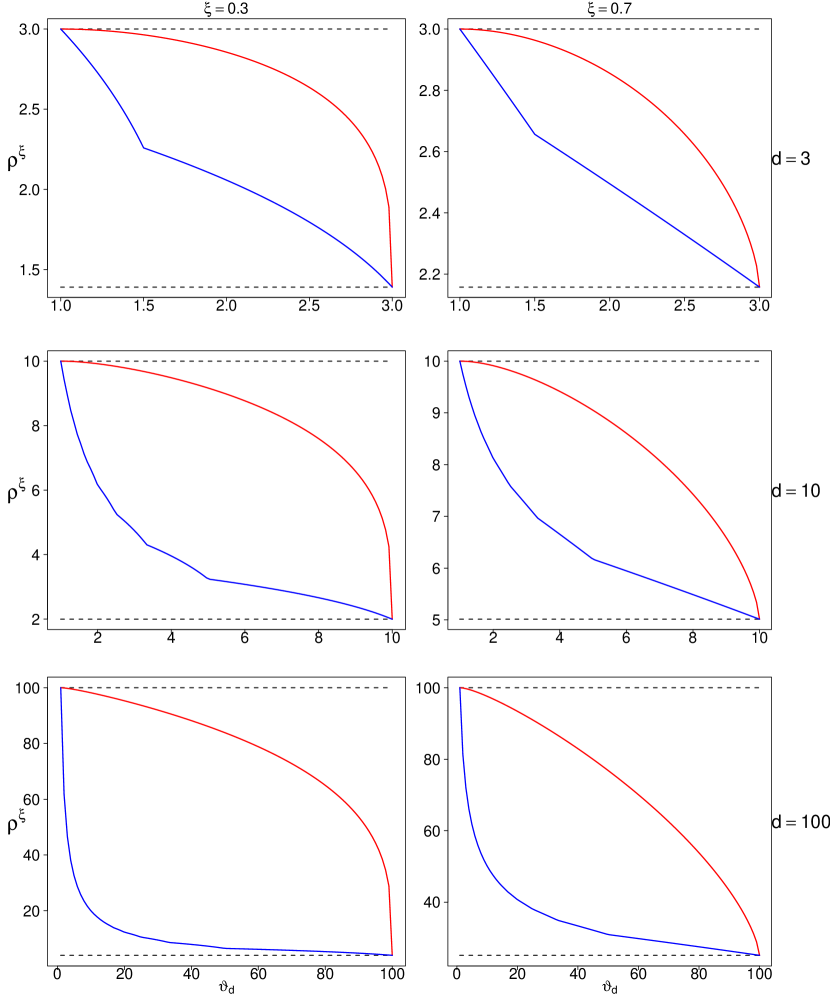
Figure 1: Upper and lower bounds on extreme VaR $\rho^{\xi}$ when given a single fixed $d$-variate extremal coefficient $\vartheta_{d}$ constraint.

Contributions. Observe that both the objective function in (1.7) and the constraints in (1.10) are linear in the parameter $H$. The challenge is, however, that $H$ takes values in an infinite-dimensional space of measures. Our findings can be summarized by three main themes:

$\bullet$ Optimal measures have finite support. We establish structural results showing that the infimum and supremum of $\rho_{\mathbf{w}}$ are attained by discrete measures that are supported on a finite set of atoms. In each case, the number of atoms is not more than the number of constraints (Theorem 3.2). Thus, in principle, the linear infinite-dimensional problems reduce to non-linear finite-dimensional optimization problems. These results stem from a fundamental connection with the theory of linear semi-infinite optimization outlined in Section 2.2 below.

$\bullet$ A Tawn-Molchanov minimizer and a convex maximizer. Surprisingly, the infimum of $\rho_{\mathbf{w}}$ and in turn the lower bound on ${\cal X}$ is attained by measures with the same support as the celebrated Tawn-Molchanov models in Strokorb and Schlather [34]. This allows us to further reduce the optimization to a linear program, which can be solved exactly using conventional linear solvers in moderate dimension. We also establish that the maximization problem reduces to an ordinary convex optimization problem which can be solved in polynomial time within arbitrary precision. Efficient solvers for these optimization problems have yet to be implemented, nevertheless our theoretical results suggest that they can be efficiently solved.

$\bullet$ Closed form solutions. Finally, in the case of a single $d$-variate constraint, we establish closed form expressions for both the lower- and upper-bounds, which are valid in arbitrary dimensions. These formulae were used in Figure 1 and further leveraged in Section 4.2 to illustrate how conditional independence can lead to very substantial reduction of the range of extreme VaR.

The rest of the paper is structured as follows. Section 2 reviews key results from the theory of linear semi-infinite programming (LSIP) and demonstrates that our optimization problem can be viewed as a dual of a LSIP. This connection is further explored in Section 3, where the main results on the general characterization of the spectral measures attaining the minimum and maximum extreme VaR are presented. Section 3.2 proceeds with more detailed results on in the cases of the Tawn-Molchanov minimizer and our closed form solutions. Section 4 briefly illustrates the established theory. In Section 4.1, using a data set of industry portfolia, we show how utilizing all bi-variate extremal coefficient constraints can lead to tight bounds on extreme VaR, which are in close agreement with semi-parametric estimates obtained using Extreme Value Theory. In Section 4.2, we provide a practical application of the closed-form formulae for the bounds on extreme VaR in a context of a market and sectors model. This demonstrates, how expert knowledge on the structure of the market can be encoded via extremal coefficient constraints in cases where data may be scarce. The proofs and auxiliary facts from optimization are collected in the Appendix.

2 A Connection to Linear Semi-Infinite Programming

In this section, we will show that our optimization problems are in fact duals to linear semi-infinite programming (LSIP) problems. This will lead to profound structural results and certain closed-form solutions for upper and lower bounds on extreme VaR.

2.1 Problem formulation

Recall that we want to solve the pair of optimization problems:

$$(\mathcal{L}_{\rho})\quad\quad\quad \inf_{H}\rho_{\mathbf{w}}(H,\xi)$$ (2.1)

$$(\mathcal{U}_{\rho})\quad\quad\quad \sup_{H}\rho_{\mathbf{w}}(H,\xi)$$ (2.2)

subject to: $$\int_{\mathbb{S}_{+}}\max_{j\in J}\{u_{j}\}H(d\boldsymbol{u})=c_{J},\text{ for all }J\in\mathcal{J},$$ (2.3)

where ${\cal J}\subset 2^{\{1,\cdots,d\}}$, is a collection of non-empty subsets of indices $\{1,\cdots,d\}$; the functional $\rho_{\mathbf{w}}$ is in (1.7); and the supremum and infimum are taken over all finite measures $H$ on $\mathbb{S}_{+}$ that satisfy the extremal coefficient constraints in (2.3).

Remark 2.1.

A set of non-negative constants $\boldsymbol{c}=(c_{J})_{J\subset\{1,\ldots,d\}}\in\mathbb{R}_{+}^{2^{d}-1}$ can be the extremal coefficients of a random vector $\mathbf{X}$, if and only if they satisfy the consistency relationships

$$\boldsymbol{c}\in\varTheta:=\left\{\boldsymbol{\vartheta}\in\mathbb{R}_{+}^{2^{d}-1}:\sum_{L\,:\,J\subseteq L}(-1)^{|L\setminus J|+1}\vartheta(L)\geq 0,\ \text{for all }J\subsetneq\{1,\ldots,d\}\right\}.$$

See Corollary 5 in [32] and [34] for more details.

Extremal coefficients are only summary, moment-type functionals, and they alone do not fully characterize the spectral measure $H$, except in special cases [34]. In general, however, it is not known to what extent the full or partial knowledge of the extremal coefficients confine the set of possible values of $\rho_{\mathbf{w}}$ and hence extreme VaR. This is one of the motivations for our work.

Assumption 2.2.

We assume that the marginal constraints (1.8) are always included in (2.3) by requiring that the singletons $\{1\},\ldots,\{d\}$ belong to $\mathcal{J}$ and $c_{\{j\}}=1$ for $j=1,\ldots,d.$ To avoid further situations that result in trivial optimization problems, we also assume $\mathcal{J}$ is sufficiently rich such that

$$1=\sum_{j=1}^{d}u_{j}<\sum_{J\in\mathcal{J}}\max_{j\in J}\{u_{j}\},\ \text{for all }\boldsymbol{u}\in\mathbb{S}_{+}.$$

In particular, this holds if $\mathcal{J}$ includes all pairs or the set $\{1,\ldots,d\}\in\mathcal{J}$.

2.2 Linear semi-infinite programming

The purpose of this section is to review definitions and notations from the field of linear semi-infinite programming (LSIP) that we will use throughout this paper (see also Appendix B.1). Our main contributions in the following Section 3 such as the existence of solutions to $(\mathcal{L}_{\rho})$ and $(\mathcal{U}_{\rho})$ with finite support (reducibility) and and exact formulae for the optimum will leverage powerful results from this established theory. Those interested in a more comprehensive treatment is referred to the monograph of Goberna and Lopez [16] as well as the review by Shapiro [33]. See also [15] for a survey of recent advancements in LSIP.

Formulation. Linear semi-infinite programs are formulated as follows:

$$(P)\quad\quad\quad\quad\inf_{\boldsymbol{x}\in\mathbb{R}^{p}} \boldsymbol{c}^{\top}\boldsymbol{x}$$

subject to: $$b(t)-\boldsymbol{a}(t)^{\top}\boldsymbol{x}\leq 0,\ t\in T,$$

where $T$ is a (possibly infinite) index set. For a given mathematical program, say $(\tilde{P})$, we use the notation $\text{val}(\tilde{P}),$ to denote its optimal value while $\text{sol}(\tilde{P})$ denotes the solution set, i.e. the set of feasible points that yield optimal values. Generally, $\text{val}(\tilde{P})$ may be infinite and $\text{sol}(\tilde{P})$ my be empty. If $\text{sol}(\tilde{P})=\varnothing$, then by convention $\text{val}(\tilde{P})=\infty$ and we say $(\tilde{P})$ is unsolvable.

The following assumption establishing the continuity of $(P)$ (in the language of LSIPs) has far reaching consequences in terms of the structure of solutions to $(P)$.

Assumption 2.3.

In $(P)$, we suppose $T$ is a compact subset of $\mathbb{R}^{d}$ and $\boldsymbol{a}:T\mapsto\mathbb{R}^{p}$, $b:T\mapsto\mathbb{R}$ are continuous and hence bounded on $T$.

Thus, we define the Lagrangian of problem $(P)$ as the function

$L:\mathbb{R}^{p}\times\Omega\mapsto\mathbb{R}$

$$L(\boldsymbol{x},\omega)=\boldsymbol{c}^{\top}\boldsymbol{x}+\int_{T}\left(b(t)-\boldsymbol{a}(t)^{\top}\boldsymbol{x}\right)\omega(dt),$$ (2.4)

where $\Omega$ is the space of finite (non-negative) Borel measures on $T$.

Remark 2.4.

Assumption 2.3 allows us to express the Lagrangian function as (2.4). This follows from the fact that the topological dual space of continuous functions on the compact set $T\subset\mathbb{R}^{p}$ is indeed the space of Borel measures on $T$. For more details see e.g. Ch. 2 of [16].

Remark 2.5.

While Assumption 2.3 appears as a rather strong condition in the literature of LSIP, we will show in Section 3 that Assumption 2.3 is naturally satisfied for our main motivating problems $(\mathcal{U}_{\rho})$ and $(\mathcal{L}_{\rho})$.

Duality. We define the dual function $g:\Omega\mapsto\mathbb{R}$ as

$$g(\omega)=\inf_{\boldsymbol{x}\in\mathbb{R}^{p}}L(\boldsymbol{x},\omega).$$

The dual function yields a lower bound on the optimal value of $(P)$. Indeed, by $(P)$, for any feasible $\tilde{\boldsymbol{x}}\in\mathbb{R}^{p}$, it follows that

$$\int_{T}\left(b(t)-\boldsymbol{a}(t)^{\top}\tilde{\boldsymbol{x}}\right)\omega(dt)\leq 0,$$

which implies

$$g(\omega)=\inf_{\boldsymbol{x}\in\mathbb{R}^{p}}L(\boldsymbol{x},\omega)\leq\boldsymbol{c}^{\top}\tilde{\boldsymbol{x}}+\int_{T}\left(b(t)-\boldsymbol{a}(t)^{\top}\tilde{\boldsymbol{x}}\right)\omega(dt)\leq\boldsymbol{c}^{\top}\tilde{\boldsymbol{x}}.$$ (2.5)

The fact that the feasible $\tilde{\boldsymbol{x}}$ was arbitrary implies $g(\omega)\leq\mathrm{val}(P).$ This inequality is trivial unless $\int_{T}\boldsymbol{a}(t)\omega(dt)=\boldsymbol{c}$. Indeed, otherwise if $\int_{T}\boldsymbol{a}(t)\omega(dt)\not=\boldsymbol{c}$, then for some $\boldsymbol{x_{0}},$ we have $\mathbf{c}^{\top}\boldsymbol{x_{0}}-\int_{T}\boldsymbol{a}(t)^{\top}\boldsymbol{x_{0}}\omega(dt)<0$, and hence by Assumption 2.3, it follows that $g(\omega)=\inf_{\boldsymbol{x}\in\mathbb{R}^{p}}L(\boldsymbol{x},\omega)=-\infty$.

Therefore, only measures $\omega\in\Omega$ for which $\int_{T}\boldsymbol{a}(t)\omega(dt)=\boldsymbol{c}$ holds are of interest and they are referred to as dual feasible. Thus we arrive at the following dual problem:

$$(D)\quad\quad\quad\quad\sup_{\omega\in\Omega} \int_{T}b(t)\omega(dt)$$

subject to: $$\int_{T}\boldsymbol{a}(t)\omega(dt)=\boldsymbol{c}.$$

In view of (2.5), we have that

$$\sup_{\omega\in\Omega}\inf_{\boldsymbol{x}\in\mathbb{R}^{d}}L(\boldsymbol{x},\omega)={\rm val}(D)\leq{\rm val}(P).$$ (2.6)

A common task with many optimization problems is to determine the existence (or non-existence) of a duality gap, $|\mathrm{val}(P)-\mathrm{val}(D)|$. If $\mathrm{val}(P)=\mathrm{val}(D)$, then it suffices to solve either $(P)$ or $(D)$ to obtain the optimal value, so long as both problems are solvable. The condition $\mathrm{val}(P)=\mathrm{val}(D)$ with $\mathrm{sol}(D)\not=\varnothing$ is known as strong duality. If $(P)$ is solvable, i.e. $\mathrm{val}(P)<\infty$, then under assumption 2.3, a sufficient condition for strong duality of $(P,D)$ is Slater’s Condition, i.e. there exists $\tilde{\boldsymbol{x}}\in\mathbb{R}^{p}$ such that

$$b(t)-\boldsymbol{a}(t)^{\top}\tilde{\boldsymbol{x}}<0,\ \text{for all }t\in T.$$ (2.7)

See Theorem 2.3 in [33] for further details on Slater’s condition and strong duality for LSIPs.

The above discussion reveals a fundamental connection between the two optimization problems in (2.1) and (2.2) and the theory of LSIP.

Corollary 2.6.

The problem of finding the upper bound $(\mathcal{U}_{\rho})$ in (2.2) under extremal coefficient constraints (2.3) is the dual to an LSIP problem $(P)$, where

$$T=\mathbb{S}_{+},\quad\mathbf{a}_{J}(t)=\max_{j\in J}\,t_{j},\ J\in{\cal J},\quad b(t)=\left(\sum_{i=1}^{d}w_{i}t_{i}^{\xi}\right)^{1/\xi}\quad\mbox{ and }\quad\mathbf{c}=(c_{J})_{J\in{\cal J}}.$$

Similarly, the problem of finding the lower bound $(\mathcal{L}_{\rho})$ in (2.1) is the dual of an LSIP involving maximization, where formally ‘$\sup$’ is reduced to ‘$\inf$’ by changing the sign of the objective function.

This connection allows us to employ powerful results from the LSIP theory discussed next.

Reducibility. The following discussion lays the groundwork for establishing the finite support of optimal solutions to $(\mathcal{L}_{\rho})$ and $(\mathcal{U}_{\rho})$. Consider a finite index set $T_{m}\subset T$ with $|T_{m}|\leq m.$ Solving problem $(P)$ when the constraints are restricted to the finite set $T_{m}$ reduces to a standard linear program

$$(P_{m})\quad\quad\quad\quad\inf_{\boldsymbol{x}\in\mathbb{R}^{p}} \boldsymbol{c}^{\top}\boldsymbol{x}$$

subject to: $$b(t_{i})-\boldsymbol{a}(t_{i})^{\top}\boldsymbol{x}\leq 0,\ t_{i}=T_{m},\ i=1,\ldots,m,$$

which yields the corresponding dual

$$(D_{m})\quad\quad\quad\quad\sup_{\boldsymbol{\omega}\in\mathbb{R}_{+}^{m}} \sum_{i=1}^{m}b(t_{i})\omega_{i}$$

subject to: $$\sum_{i=1}^{m}\boldsymbol{a}(t_{i})\omega_{i}=\boldsymbol{c},\ t_{i}=T_{m},\ i=1,\ldots,m.$$

Problem $(P_{m})$ is called a discretization of $(P)$. The feasible set for $(P)$ is contained in the feasible set for $(P_{m})$. Hence, $\mathrm{val}(P_{m})\leq\mathrm{val}(P).$ If for every $\varepsilon>0$, there exists $(P_{m(\varepsilon)})$ such that $\mathrm{val}(P)-\mathrm{val}(P_{m(\varepsilon)})\leq\varepsilon$ than we say $(P)$ is discretizable. Whereas, if there exists $(P_{m})$ such that $\mathrm{val}(P_{m})=\mathrm{val}(P)$ then $(P)$ is said to be reducible. In this case, on the language of measures, the optimum is attained by a discrete measure $\omega(dt)=\sum_{i=1}^{m}\nu_{i}\delta_{\{t_{i}\}}(dt)$ with a finite support $\{t_{1},\ldots,t_{m}\}\subset T$.

Remark 2.7.

Even if an LSIP is theoretically reducible, it may be challenging to find the actual support set of an $\omega\in{\rm sol}(D)$. This is because finding the support amounts to solving a non-linear optimization problem.

The following proposition establishes conditions for the reducibility of the LSIP $(P)$.

Proposition 2.8 (Theorem 3.2 in [33]).

Suppose that for problem $(P)$, Assumption 2.3 holds and $\mathrm{val}(P)<\infty$. If for any $\{t_{1},t_{2},\ldots t_{p+1}\}\subset T$, there exists $\boldsymbol{x}\in\mathbb{R}^{p}$ such that

$$\boldsymbol{a}(t_{k})^{\top}\boldsymbol{x}>b(t_{k}),\ k=1,\ldots,p+1.$$ (2.8)

Then there exists $\{t_{1},\ldots,t_{m}\}=T_{m}\subset T$ with $m\leq p$ such that for corresponding discretizations $(P_{m})$ and $(D_{m})$

$$\mathrm{val}(P)=\mathrm{val}(P_{m})=\mathrm{val}(D_{m})=\mathrm{val}(D).$$

Note that if Slater’s condition holds for $(P)$, then (2.8) is satisfied. Which yields the following corollary

Corollary 2.9.

If Assumption 2.3 holds for $(P)$, $\mathrm{val}(P)<\infty$ and Slater’s condition holds, then there exists a (strong) dual pair $(P,D)$ and $\omega\in\mathrm{sol}(D)\subset\Omega$ such that $\omega$ is finitely supported on at most $p$ atoms $\{t_{1},t_{2},\ldots,t_{p}\}\subset T$.

3 Main results

3.1 Optimal measures with finite support

In this section, we establish general structural results for problems $(\mathcal{L}_{\rho})$ and $(\mathcal{U}_{\rho})$ by exploiting their duality to linear semi-infinite programs (LSIPs) discussed above. We show that the optimum are attained by measures with finite support and we prove that $(\mathcal{U}_{\rho})$ is equivalent to a finite dimensional convex optimization problem, which can be solved in polynomial time.

Theorem 3.1.

If Assumption 2.2 holds, then there exist (primal) linear semi-infinite programs $(\mathcal{L}_{\rho}^{\prime})$ and $(\mathcal{U}_{\rho}^{\prime})$, whose dual problems are $(\mathcal{L}_{\rho})$ and $(\mathcal{U}_{\rho})$, respectively. Furthermore, for $(\mathcal{L}_{\rho}^{\prime})$ and $(\mathcal{U}_{\rho}^{\prime})$, we have:

(i) Assumption 2.3 is satisfied.

(ii) The Slater condition holds.

(iii) The optimal values are finite.

(iv) Strong duality holds for the pairs $(\mathcal{L}_{\rho},\mathcal{L}_{\rho}^{\prime})$ and $(\mathcal{U}_{\rho},\mathcal{U}_{\rho}^{\prime})$.

(v) The problems are reducible.

(vi) There exists solutions to $(\mathcal{L}_{\rho})$ and $(\mathcal{U}_{\rho})$ that are supported on at most $|\mathcal{J}|$ atoms.

Proof.

We consider only problems $(\mathcal{U}_{\rho})$ and $(\mathcal{U}_{\rho}^{\prime})$. The arguments for $(\mathcal{L}_{\rho})$ and $(\mathcal{L}_{\rho}^{\prime})$ are similar.

Let $p=|\mathcal{J}|$ and $\boldsymbol{c}=(c_{J})_{J\in\mathcal{J}}\in\mathbb{R}_{+}^{p}.$ Define the continuous functions $b:\mathbb{S}_{+}\mapsto\mathbb{R}_{+}$, $\boldsymbol{a}:\mathbb{S}_{+}\mapsto\mathbb{R}_{+}^{p}$

$$b(\boldsymbol{u})=\left(w_{1}u_{1}^{\xi}+\cdots+w_{d}u_{d}^{\xi}\right)^{1/\xi}\quad\mbox{ and }\quad\boldsymbol{a}(\boldsymbol{u})=\left(\max_{j\in J}\{u_{j}\}\right)_{J\in\mathcal{J}}.$$

Consider the linear semi-infinite program

$$(\mathcal{U}_{\rho}^{\prime})\quad\quad\quad\quad\inf_{\boldsymbol{x}\in\mathbb{R}^{p}} \boldsymbol{c}^{\top}\boldsymbol{x}$$ (3.1)

subject to: $$b(\boldsymbol{u})-\boldsymbol{a}(\boldsymbol{u})^{\top}\boldsymbol{x}\leq 0,\ \boldsymbol{u}\in\mathbb{S}_{+}.$$

Letting $\mathcal{H}$ denote the space of finite Borel measures on $\mathbb{S}_{+}$, by the Lagrangian duality theory discussed in Section 2.2, it follows that the dual of $(\mathcal{U}_{\rho}^{\prime})$ is

$$\quad\quad\quad\quad\sup_{H\in\mathcal{H}} \int_{\mathbb{S}_{+}}\left(w_{1}u_{1}^{\xi}+\cdots+w_{d}u_{d}^{\xi}\right)^{1/\xi}H(d\boldsymbol{u})$$

subject to: $$\left\{\int_{\mathbb{S}_{+}}\max_{j\in J}\{u_{j}\}H(d\boldsymbol{u})=c_{J}\right\}_{J\in\mathcal{J}},$$

which is in fact problem $(\mathcal{U}_{\rho})$ in (2.2). This establishes the desired duality of $(\mathcal{U}_{\rho})$ to the above LSIP $(\mathcal{U}_{\rho}^{\prime})$.

Now, observe that $(\mathcal{U}_{\rho}^{\prime})$ satisfies Assumption 2.3, since $\mathbb{S}_{+}\subset\mathbb{R}^{d}$ is compact and the functions $b$ and $\boldsymbol{a}$ are continuous on $\mathbb{S}_{+}$. This proves (i).

We next show (ii). Observe that for all $\boldsymbol{u}\in\mathbb{S}_{+},$ we have

$$b(\boldsymbol{u}) = \left(w_{1}u_{1}^{\xi}+\cdots+w_{d}u_{d}^{\xi}\right)^{1/\xi}\leq{\Big{(}}\max_{j=1,\dots,d}w_{j}^{1/\xi}{\Big{)}}\sum_{j=1}^{d}u_{j}$$ (3.2)

$$=: C_{\mathbf{w}}\sum_{j=1}^{d}u_{j}<C_{\mathbf{w}}\boldsymbol{a}(\boldsymbol{u})^{\top}\boldsymbol{1},$$

where inequality in (3.2) follows from Assumption 2.2. Hence $\tilde{\boldsymbol{x}}\equiv C_{\mathbf{w}}\mathbf{1}\in\mathbb{R}^{p}$ is primal feasible for the LSIP program $(\mathcal{U}_{\rho}^{\prime})$ and the Slater condition (2.7) holds.

In view of (1.9), (2.6), and (3.2), we obtain

$$-\infty<{\Big{(}}\sum_{i=1}^{d}w_{i}{\Big{)}}^{1/\xi}\leq\mathrm{val}(\mathcal{U}_{\rho})\leq\mathrm{val}(\mathcal{U}_{\rho}^{\prime})\leq C_{\mathbf{w}}\sum_{J\in\mathcal{J}}c_{J}<\infty,$$

which proves (iii).

Finally, by Proposition 2.8 (c.f. Corollary 2.9), (i), (ii), and (iii) are sufficient for (iv), (v), and (vi). ∎

The fact that Theorem 3.1(vi) implies that the optimal values of $(\mathcal{L}_{\rho})$ and $(\mathcal{U}_{\rho})$ can be achieved by measures concentrated on at most $|{\cal J}|$ atoms leads to the following characterization of ${\rm val}(\mathcal{L}_{\rho})$ and ${\rm val}(\mathcal{U}_{\rho})$.

Theorem 3.2.

Recall the extremal coefficient constraints $\boldsymbol{c}=(c_{J})_{J\in\mathcal{J}}\in\mathbb{R}^{|\mathcal{J}|}_{+}$ in (2.3) for problems $(\mathcal{L}_{\rho})$ and $(\mathcal{U}_{\rho})$. Define the set of non-negative $d\times|{\cal J}|$ matrices

$$\mathcal{A}_{\boldsymbol{c}}:=\left\{A\in\mathbb{R}_{+}^{d\times|\mathcal{J}|}\,:\,\sum_{K\in\mathcal{J}}\max_{j\in J}\{a_{jK}\}=c_{J},J\in\mathcal{J}\right\}.$$ (3.3)

Then, by letting $f(A):=\sum_{K\in{\cal J}}\left(w_{1}a_{1K}^{\xi}+\cdots+w_{d}a_{dK}^{\xi}\right)^{1/\xi}$, we have

$${\rm val}(\mathcal{L}_{\rho})=\inf_{A\in\mathcal{A}_{\boldsymbol{c}}}f(A)\quad\mbox{ and }\quad{\rm val}(\mathcal{U}_{\rho})=\sup_{A\in\mathcal{A}_{\boldsymbol{c}}}f(A).$$

Proof.

Theorem 3.1(vi) implies that there exists a discretization $(\mathcal{L}_{\rho}^{m})$ with $m\leq|\mathcal{J}|$ such that $\mathrm{val}(\mathcal{L}_{\rho}^{m})=\mathrm{val}(\mathcal{L}_{\rho})<\infty.$ The last statement means that there exist $\boldsymbol{u}_{k}\in\mathbb{S}_{+},h_{k},\ k=1,\ldots,m$ such that

$$\mathrm{val}(\mathcal{L}_{\rho})= \inf_{{\boldsymbol{u}_{k}\in\mathbb{S}_{+}\atop h_{k}\geq 0}}\sum_{k=1}^{m}\left(w_{1}u_{1k}^{\xi}+\cdots+w_{d}u_{dk}^{\xi}\right)^{1/\xi}h_{k}$$ (3.4)

$$\mathrm{subject\ to}:\ \left\{\sum_{k=1}^{m}\max_{j\in J}\{u_{jk}\}h_{k}=c_{J}\right\}_{J\in\mathcal{J}}.$$

making the change of variables $a_{jk}=u_{jk}h_{k}$ gives

$$\mathrm{val}(\mathcal{L}_{\rho})= \inf_{a_{jk}\geq 0}\sum_{k=1}^{m}\left(w_{1}a_{1k}^{\xi}+\cdots+w_{d}a_{dk}^{\xi}\right)^{1/\xi}$$

$$\mathrm{subject\ to}:\ \left\{\sum_{k=1}^{m}\max_{j\in J}\{a_{jk}\}=c_{J}\right\}_{J\in\mathcal{J}}.$$

Thus we have proved the result for $(\mathcal{L}_{\rho}).$ The proof for $(\mathcal{U}_{\rho})$ follows by replacing $\sup_{A\in\mathcal{A}_{\boldsymbol{c}}}f(A)$ with $\inf_{A\in\mathcal{A}_{\boldsymbol{c}}}-f(A)$. ∎

The consequence of Theorem 3.2 is that the linear semi-infinite optimization problems $(\mathcal{L}_{\rho})$ and $(\mathcal{U}_{\rho})$ may be reduced to finite yet non-linear optimization problems. Fundamentally, there is tradeoff between linearity in the semi-infinite case, versus non-linearity in the finite case, amounting to having to search for the finite support of the optimal measures in $\mathrm{sol}(\mathcal{L}_{\rho})$ and $\mathrm{sol}(\mathcal{U}_{\rho})$. This is because both the objective function and the constraints now depend on the unknown set of support points $T_{m}:=\{{\bf u}_{1},\cdots,{\bf u}_{m}\}$, in Relation (3.4) in a non-linear fashion. Note however that the size of the unknown support $T_{m}$ is no greater than the number of constraints, which is one of the appealing consequences of Theorem 3.1 (vi).

In the case of $(\mathcal{U}_{\rho})$, $\xi<1$ implies that $-f(A)$ is a convex function. This, together with the fact that $\mathcal{A}_{\boldsymbol{c}}$ is a convex set means that $\inf_{A\in\mathcal{A}_{\boldsymbol{c}}}-f(A)$ is a convex optimization problem. Hence $\inf_{A\in\mathcal{A}_{\boldsymbol{c}}}-f(A)$ can be solved to within arbitrary precision in polynomial time[6]. In-practice, an exact and efficient solver for $\inf_{A\in\mathcal{A}_{\boldsymbol{c}}}-f(A)$ still needs to be developed and is outside the scope of this work.

In the case of $(\mathcal{L}_{\rho})$, $\xi<1$ implies $\inf_{A\in\mathcal{A}_{\boldsymbol{c}}}f(A)$ is non-convex and generally more challenging. However, if one makes a further assumption of balanced portfolio, i.e. the weights in $f$ are equal $w_{1}=w_{2}=\cdots=w_{d}=1$, then further solutions are readily available as discussed in the following section.

3.2 Solutions for balanced portfolia

In this section, we provide further structural results and closed form solutions in the important special case of balanced portfolia, where $\mathbf{w}={\bf 1}$:

$$w_{1}=w_{2}=\cdots=w_{d}=1.$$ (3.5)

Remark 3.3.

Under assumption (3.5), the universal dependence bounds for extreme VaR ${\cal X}_{(S,X_{1})}=\rho_{\bf 1}^{\xi}$ given by (1.9) simplify to

$$d^{\xi}\leq{\cal X}_{(S,X_{1})}\leq d.$$

We show first that the minimization problem $(\mathcal{L}_{\rho})$ reduces to a standard linear program. Interestingly, ${\rm val}(\mathcal{L}_{\rho})$ is attained by spectral measures corresponding to the celebrated Tawn-Molchanov max-stable models [34]. This leads to efficient and exact solutions in practice for moderate number of constraints and dimensions.

The second contribution are exact formulae for both the lower and upper bounds on $\rho:=\rho_{\bf 1}$ in the case when we impose only one constraint on the $d$-variate extremal coefficient

$$\vartheta=\vartheta_{\mathbf{X}}(\{1,\ldots,d\}),$$

in addition to the standard marginal extremal coefficient constraints. These results are possible thanks to the symmetry in the objective function when all portfolio weights are equal. Their proofs are given in Appendix B.

Theorem 3.4 (Tawn-Molchanov Minimizer).

Under assumption (3.5), we have

$$\mathrm{val}(\mathcal{L}_{\rho}) = \inf_{\boldsymbol{\beta}\in\mathbb{R}_{+}^{2^{d}-1}}\sum_{J\subset\{1,\ldots,d\},\ J\not=\varnothing}|J|^{1/\xi}\beta_{J}$$

$$\mathrm{subject\ to}:\left\{\sum_{K\subset\{1,\ldots,d\},\ K\not=\varnothing}\mathbb{I}\left\{(K\cap J)\not=\varnothing\right\}\beta_{K}=c_{J}\right\}_{J\in\mathcal{J}}.$$

This result shows that obtaining the lower bound for extreme VaR in the case of a balanced portfolio amounts to solving a high-dimensional but standard linear program.

Remark 3.5.

From the proof of Theorem 3.4, it follows that the lower bounds for extreme VaR in balanced portfolia are attained by spectral measures supported on the set of vectors

$$\left\{|J|^{-1}(\boldsymbol{1}_{J}(j))_{j=1}^{d}:J\subset\{1,\ldots,d\}\right\}\subset\mathbb{S}_{+}.$$

Such types of spectral measures correspond to the Tawn-Molchanov max-stable model [34]. This is an interesting finding since, as shown in the last reference, the Tawn-Molchanov max-stable models are maximal elements with respect to the lower orthant stochastic order, for the set of all max-stable distributions sharing a fixed set of extremal coefficients. Theorem 3.4, however, is not a consequence of the lower orthant order dominance and its proof is based on optimization results.

Remark 3.6 (terminology).

According to a personal communication with Dr. Kirstin Strokorb, the Tawn-Molchanov or more completely Schlather-Tawn-Molchanov max-stable model originates in the works of [32] and [23]. In the work [24] it is shown to arise from a Choquet integral and is therefore more descriptively referred to as a Choquet max-stable model.

Closed form solutions. Next, we focus on the case of a single constraint, involving the extremal coefficient associated with the entire set $D=\{1,\ldots,d\}.$ That is, the extremal coefficient constraints (2.3) in $(\mathcal{L}_{\rho})$ and $(\mathcal{U}_{\rho})$ are given by

$$\mathcal{J}=\mathcal{J}_{d}:=\{\{1\},\{2\},\ldots,\{d\},D\}\quad\mbox{ and }\quad\boldsymbol{c}=\boldsymbol{c}_{\vartheta}:=(1,1,\ldots,1,\vartheta)\in\mathbb{R}_{+}^{d+1},$$ (3.7)

where $\vartheta=\vartheta_{\mathbf{X}}(D)\in[1,d]$. The following results show that in this special case, exploiting the symmetry in the constraints yields closed form solutions for both ${\rm val}(\mathcal{L}_{\rho})$ and ${\rm val}(\mathcal{U}_{\rho})$.

Theorem 3.7 (lower bounds).

Let $B_{k}=[d(k+1)^{-1},dk^{-1})$, $k=1,\ldots,d-1.$ Under assumption (3.7), for all $\vartheta\in[1,d]$, we have that ${\rm val}(\mathcal{L}_{\rho})$ is given by the piecewise linear function:

$${\rm val}(\mathcal{L}_{\rho})=L(\vartheta):=\sum_{k=1}^{d-1}\boldsymbol{1}_{B_{k}}(\vartheta)\left\{\frac{k{}^{1/\xi-1}-(k+1)^{1/\xi-1}}{k^{-1}-(k+1)^{-1}}\left(\vartheta-\frac{d}{k+1}\right)+d(k+1)^{1/\xi-1}\right\}.$$ (3.8)

Theorem 3.8 (upper bounds).

Under assumption (3.7), for all $\vartheta\in[1,d]$, we have

$${\rm val}(\mathcal{U}_{\rho})=U(\vartheta):=\left\{\vartheta^{\xi}+(d-1)^{1-\xi}(d-\vartheta)^{\xi}\right\}^{1/\xi}\equiv\sup_{\boldsymbol{u}\in\mathbb{S}_{+}}\left\{d\left(\sum_{j=1}^{d}u_{j}^{\xi}\right)^{1/\xi}:\max_{j\in D}\{u_{j}\}=\frac{\vartheta}{d}\right\}.$$ (3.9)

The bounds in (3.8) and (3.9) can be computed for arbitrary dimension and all tail index values $\xi\in(0,1]$. The results shown in Figure 1 show that the information about extreme VaR provided by a single d-variate extremal coefficient increases with the tail index $\xi$ and decreases with dimension $d$. More concretely, computing the maximum width of the bounds $\sup_{\vartheta\in[1,d]}|\mathrm{val}(\mathcal{U}_{\rho})^{\xi}-\mathrm{val}(\mathcal{L}_{\rho})^{\xi}|$ using the closed form solutions and comparing to the width of the universal dependance bounds $|d-d^{\xi}|$ allow us to show that even in the high-dimensional setting of $d=100$, with realistic tail exponent $\xi=0.7$, the knowledge of a single $d$-variate extremal coefficient always reduces the range of uncertainty of extreme VaR by at least $29\%$. This is a remarkable fact given that no other assumptions on the asymptotic dependence are imposed.

4 Applications

The goal of this section is to briefly illustrate the theoretical structural results as well as closed-form formulae established above. We start with a quantitative example of a $10$-dimensional industry portfolio, where the bi-variate constraints are estimated from data. Then, in Section 4.2, we demonstrate how extremal coefficient constraints can be used to encode qualitative structural information and arrive at practical closed-form formulae.

4.1 An illustration: Scale-balanced industry portfolia

In this section, we briefly sketch an application of the above general results using a $d=10$-dimensional portfolio of daily returns for $10$ industries available in [14]. The portfolio is obtained by assigning each of the stocks in NYSE, AMEX, and NASDAQ to one of the ten industries and then their average is computed. Then, a vector time-series of daily returns in percent are computed. We shall focus on the vector time-series $\mathbf{X}_{t}=(X_{t}(j))_{j=1}^{d}$ of losses (negative returns) and study their extreme value-at-risk. We first argue that it is reasonable to model the (multivariate) marginal distribution as regularly varying. To this end, we briefly recall the standard peaks-over-threshold methodology used to estimate the tail index and scale of the losses.

Let the random variable $X$ represent the loss of an asset. The Pickands-Balkema-de Haan Theorem (see e.g. Theorem 3.4.13 and page 166 in [11]) implies that under general conditions, there exist normalizing constants $\sigma(u)>0$, such that

$$\mathbb{P}\left(\frac{X-u}{\sigma(u)}>x\,{\Big{|}}\,X>u\right)\to(1+\xi x)_{+}^{-1/\xi},$$

as $u\to x^{*}$, where $x^{*}:=\sup\{x\,:\,\mathbb{P}(X>x)>0\}\in(-\infty,+\infty]$ is the upper end-point of the distribution of $X$. Here $\xi\in\mathbb{R}$ is a shape parameter referred to as the tail index and $(x)_{+}:=\max(0,x)$. This result suggests that the conditional distribution of the distribution of the excess $X-u$ over a large threshold $u$ can be approximated with the so-called Generalized Pareto (GP) distribution, i.e.,

$$\mathbb{P}(X-u>x|X>u)\approx\left(1+\xi\frac{x}{\sigma(u)}\right)_{+}^{-1/\xi}.$$

The case $\xi>0$ corresponds to heavy, power-law tails; $\xi=0$ (interpreted by continuity) is the Exponential distribution and $\xi<0$ is a distribution with bounded right tail. In practice, one picks a large threshold $u$, focuses on the part of the sample exceeding $u$, and estimates the tail index $\xi$ and scale parameter $\sigma=\sigma(u)$ via maximum likelihood applied to the excesses. (In the presence of significant temporal dependence, extremes tend to cluster, i.e., losses occur in batches. In this case, an important methodological step is to de-cluster the exceedances, i.e., to pick one observation from each cluster or otherwise reduce the dependence (see, e.g., [7]). In our case, declustering had virtually no effect on the estimates.

Table 1 shows the tail index and scale estimates along with their standard errors for each of the $10$ industries. They were obtained by fitting a GP model via the method of maximum likelihood to the excesses over the $0.98$th empirical quantile, for each of the $10$ daily loss time series. The first important observation is that all losses are heavy tailed, where the tail index estimates are not significantly different. Indeed, the p-value of a chi-square test for equality of means applied to the $10$ tail index estimates (assuming normal approximation) is $0.81$. On the other hand, the scales are significantly different with p-value $1.7\times 10^{-12}$. While these marginal estimators are dependent and the chi-square test is likely to be conservative. Therefore, with some confidence we can assume that the daily losses have a common tail index $\xi$ and are multivariate regularly varying. Furthermore, the GP tail asymptotics entail

$$\mathbb{P}(X_{t}(j)>x)\sim p_{0}\left(\frac{\sigma_{j}}{\xi}\right)^{1/\xi}x^{-1/\xi},\ \ \mbox{ as }x\to\infty,$$ (4.1)

where $p_{0}:=1-0.98=0.02$.

Table 1: Tail index and scale estimates based on a MLE of a GPD model to peaks over the $0.98$-th marginal quantiles of industry losses.

	$\widehat{\xi}$	${\rm s.e.}({\widehat{\xi}})$	$\widehat{\sigma}$	${\rm s.e.}(\widehat{\sigma})$
NoDur	0.21	0.06	0.77	0.05
Durbl	0.18	0.06	1.32	0.10
Manuf	0.22	0.06	1.06	0.08
Enrgy	0.19	0.05	1.05	0.07
HiTec	0.13	0.05	1.29	0.09
Telcm	0.22	0.05	0.84	0.06
Shops	0.20	0.06	0.92	0.07
Hlth	0.25	0.06	0.92	0.07
Utils	0.14	0.05	1.21	0.08
Other	0.14	0.06	1.25	0.09

In order to apply our closed-form solutions from Section 3.2, we consider the balanced portfolio

$$S_{t}:=\sum_{j=1}^{d}w_{j}X_{t}(j),\ \ \mbox{ with }w_{j}\propto\frac{1}{\widehat{\sigma}_{j}},$$

where $\sum_{j=1}^{d}w_{j}=1$. Thus, the scales of all assets are balanced so that $\mathbb{P}(w_{j}X_{t}(j)>x)\sim\mathbb{P}(w_{1}X_{t}(1)>x)$ as $x\to\infty$. Figure 2 (left) shows the time series of daily losses for the scale-balanced portfolio. The right panel therein shows the empirical value-at-risk as a function of $\alpha:=1-q$ for the balanced as well as for the equally weighted portfolio $\widetilde{S}_{t}:=d^{-1}\sum_{j=1}^{d}X_{t}(j)$.

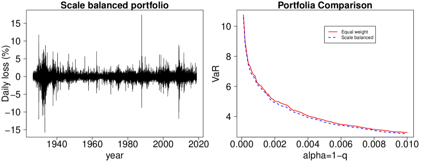
Figure 2: Left panel: Time series of daily losses for the scale-balanced portfolio. Right panel: empirical value-at-risk as a function of $\alpha=1-q$ for the scale-balanced and equally weighted portfolia.

Observe that the VaR of the balanced portfolio is always lower (by about 1% to 4.5%) for a wide range of risk levels $q$. This difference is significant and indicates that the balanced portfolio is preferable in practice. The reduction of risk may be explained by the fact that the extremal dependence in the assets is relatively balanced. Had there been a group of industries which were significantly more dependent than the rest, the scale-balanced portfolio might not have outperformed the equally weighted one. In such a case, one should balance the marginal risk (through the scales) as well as consider diversification due to extremal dependence. Such portfolio optimization problems can be considered with the same tools that we employed here but they go beyond the scope of the present study.

Now, for the scale-balanced portfolio, the marginal constraints are met and one has

$${\rm VaR}_{q}(S_{t})\sim\chi\times{\rm VaR}_{q}(w_{1}X_{t}(1)),\ \ \mbox{ as }q\to 1,$$ (4.2)

where $\chi=\rho^{\xi}$ with $\rho=\rho_{\bf 1}$ as in (1.7). Theorems 3.7 and 3.8 yield closed-form expressions for the upper and lower bounds on $\rho$ as a function of the single $d$-variate extremal index $\vartheta$. On the other hand, Theorem 3.4 shows that the lower bound on $\rho$ can be obtained by solving a linear program. We used empirical estimates of the $d$-variate and all bi-variate extremal coefficients of the scale-balanced portfolio based on the $0.98$th empirical quantiles (see Table 4 below and Section A.2 for more details). These estimates are in fact valid extremal coefficients in the sense of Remark 2.1 (see Remark A.3, below). The resulting bounds are given in Table 2. Observe that the additional information in the bi-variate extremal coefficients substantially narrows the gap between the bounds based on a single constraint. At the same time, relative to the wide Fréchet bounds, the improvement in the bounds due to single d-variate extremal coefficient is remarkable.

Table 2: Bounds on the extreme VaR coefficient $\chi=\rho_{\bf 1}^{\xi},\ \xi:=0.1981$ for the scale-balanced portfolio with $d=10$.

Constraints	Lower bound	Upper bound
Single d-variate	4.1219	9.7818
All bi-variate	6.6852	–
Fréchet bounds (no constraints)	1.5782	10

Finally, to obtain the estimate of ${\rm VaR}_{q}(S_{t})$ in (4.2), one needs to calculate the baseline ${\rm VaR}_{q}(w_{1}X_{t}(1))$. We did so using empirical quantiles and also from the Generalized Pareto tail approximation in (4.1), which entails

$${\rm VaR}_{q}(w_{1}X_{t}(1))\approx\frac{w_{1}\widehat{\xi}}{\widehat{\sigma}_{1}}\left(\frac{1-q}{p_{0}}\right)^{-\widehat{\xi}},$$

where $\widehat{\sigma}_{1}=0.77$ and $\widehat{\xi}=0.198$ is obtained through ML by assuming that the excess losses of all $10$ time series have a common tail index but different scales.

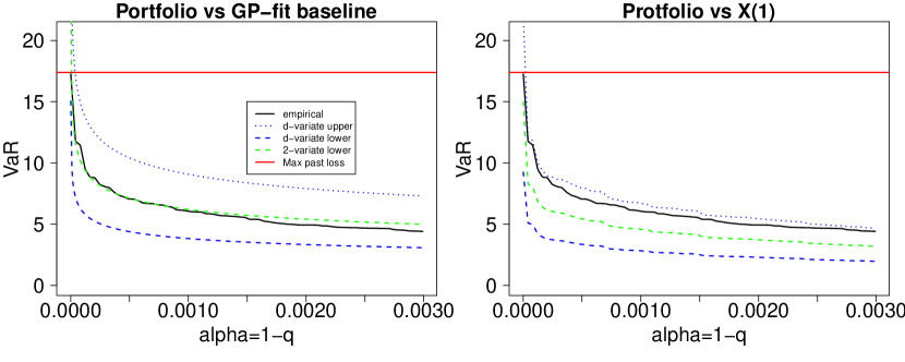
Figure 3: Upper and lower bounds on VaR as a function of $\alpha=1-q$ based on single $d$-variate and all bi-variate extremal coefficient constraints. The solid line indicates the empirical VaR. Left panel: bounds are relative to the Generalized Pareto model-fit baseline. Right panel: bounds are relative to the empirical VaR of the non-durable goods industry.

Figure 3 shows the upper and two types of lower bounds on ${\rm VaR}_{q}(S_{t})$ as a function of $\alpha=1-q$. The empirical portfolio VaR is also given (solid line). The bounds in the left panel are relative to the baseline value-at-risk computed from the Generalized Pareto model approximation, while in the right panel ${\rm VaR}_{q}(w_{1}X_{t}(1))$ is replaced by the corresponding empirical quantile. Relative to the GP-fit baseline, the empirical portfolio VaR is within the upper and the larger lower bound (green dashed line) for extreme loss levels $\alpha<0.001$. It falls slightly below the lower bound based on bi-variate extremal coefficient constraints for less-extreme loss levels, which can be attributed to both variability in the constraints estimates and uncertainty in the GP model. Nevertheless, the agreement is remarkable, especially for extreme loss levels where the asymptotic approximation kicks-in. In the right panel the bounds are relative to the empirical value-at-risk baseline. In this case, the portfolio VaR is always enclosed between the bi-variate lower bound and the d-variate upper bound and in fact the gap between them is more narrow relative to that in the left panel. This illustrates that the asymptotic approximation is quite accurate for a wide range of extreme quantiles and that the extremal coefficient constraints capture well the extremal dependence between the assets in the portfolio. One advantage of the GP-fit baseline however is that one can extrapolate the bounds on the portfolio VaR beyond the historically available quantile levels.

Table 3: Bounds on the return levels for the scale-balanced portfolio. VaR_q with $1-q=1/(252\times m)$ is exceeded on the average once in every $m$ years.

Return levels (years)	10	100	1000
d-variate upper	10.90	17.20	27.14
d-variate lower	4.59	7.25	11.44
bi-variate lower	7.45	11.75	18.55

Indeed, Table 3 provides bounds on the $10$, $100$ and $1000$-year return levels, where a year is assumed to have $252$ trading days. These results indicate for example that one should expect to encounter daily losses exceeding $4.59\%$ once in $10$ years on the average, even for the relatively diversified scale-balanced portfolio, but daily losses of $17.2\%$ or more are unusual 1-in-a-100 year type events. Even though these results hinge on the assumption of stationarity in the extremal dependence structure, they provide novel distributionally robust bounds of extreme portfolio or insurance risk and can be used to validate most if not all other model-based estimators of extreme value-at-risk.

Table 4: Empirical estimates for the bivariate extremal coefficients $\widehat{\vartheta}(\{i,j\})$ for the scale-balanced 10-industry potfolio based on exceedances over the $0.98$th quantiles. See (A.8). The single $d$-variate extremal coefficient estimate based on the same quantile is $\widehat{\vartheta}(\{1,\dots,d\})=3.15$.

	NoDur	Durbl	Manuf	Enrgy	HiTec	Telcm	Shops	Hlth	Utils	Other
NoDur	1.00	1.46	1.37	1.50	1.48	1.54	1.38	1.44	1.48	1.40
Durbl	1.46	1.00	1.30	1.50	1.46	1.58	1.44	1.57	1.46	1.35
Manuf	1.36	1.29	1.00	1.43	1.40	1.53	1.36	1.49	1.40	1.26
Enrgy	1.49	1.50	1.43	1.00	1.60	1.61	1.52	1.60	1.54	1.47
HiTec	1.48	1.45	1.40	1.60	1.00	1.55	1.43	1.55	1.47	1.45
Telcm	1.53	1.58	1.54	1.61	1.55	1.00	1.55	1.60	1.61	1.52
Shops	1.37	1.44	1.36	1.52	1.43	1.55	1.00	1.48	1.47	1.38
Hlth	1.43	1.56	1.49	1.60	1.55	1.60	1.48	1.00	1.60	1.54
Utils	1.47	1.46	1.40	1.55	1.47	1.61	1.47	1.60	1.00	1.44
Other	1.39	1.35	1.26	1.47	1.45	1.52	1.38	1.54	1.44	1.00

4.2 Market and sectors framework

While the quantitative methods in previous section based on the knowledge of all bi-variate constraints yield tight bounds, their use in practice is limited to small and moderate dimensions due to practical challenges in solving the optimization problems. In this section, our goals is two-fold. First, we illustrate how one may encode structural/expert knowledge through extremal coefficient constraints. Secondly, we show that the closed-form expressions in Theorems 3.7 and 3.8 can lead to practical and tight bounds on extreme VaR in high-dimensions, where numerical optimization is either challenging or impossible.

We do so over a simple but instructive ‘market plus sectors’ framework. Namely, suppose that the vector of portfolio losses $\mathbf{X}=(X_{1},\cdots,X_{d})$ is regularly varying with index $\xi\in(0,1)$ and standardized marginal scales in the sense of (1.5).

Let $\beta\in(0,1)$, and suppose that

$$\mathbf{X}=\beta^{\xi}\mathbf{X}_{\rm mkt}+(1-\beta)^{\xi}\mathbf{X}_{\rm sec},$$ (4.3)

where $\mathbf{X}_{\rm mkt}$ and $\mathbf{X}_{\rm sec}$ are independent and also regularly varying with index $\xi$ and asymptotically standardized margins (as in (1.5)). The components $\mathbf{X}_{\rm mkt}$ and $\mathbf{X}_{\rm sec}$ represent the overall market and individual sector-specific risks, respectively.

We shall assume that the market risk affects all stocks and therefore model it as asymptotically completely dependent, i.e.,

$${\vartheta}_{\mathbf{X}_{\rm mkt}}(\{1,\dots,d\})=1.$$

We shall also assume that $\mathbf{X}_{\rm sec}=(\mathbf{X}(1),\dots,\mathbf{X}(k))$ is partitioned into independent sub-vectors $\mathbf{X}(i)=(X_{j}(i))_{j=1}^{d_{i}}$, each corresponding to a sector. That is, $d=d_{1}+\cdots+d_{k}$ and

$$\{1,\dots,d\}=J_{1}\cup\cdots\cup J_{d},$$

where $J_{i},\ i=1,\dots,k$ are pairwise disjoint sets of indices.

Relation (4.3) leads to a simple but natural 2-tier asymptotic dependence structure. The parameter $\beta$ controls the proportion of risk due to overall market-wide events, while the individual sectors may experience independent, and largely arbitrary internal risk exposures accounted for by the sector-specific component. We demonstrate next how the closed form formulae in Theorems 3.7 and 3.8 lead to tight lower- and upper-bounds on extreme VaR for the portfolio $\mathbf{X}$.

Using the independence of the market and the sectors, it can be shown that:

$$H_{\mathbf{X}}=\beta\times H_{\mathbf{X}_{\rm mkt}}+(1-\beta)\times\sum_{i=1}^{k}H_{\mathbf{X}(i)},$$ (4.4)

where $H$ with the corresponding sub-script is the properly normalized spectral measure of the corresponding vector $\mathbf{Z}:=\mathbf{X}^{1/\xi}$, where we naturally embed $H_{\mathbf{X}(i)}$ into the higher-dimensional space $\mathbb{S}_{+}\subset\mathbb{R}^{d}$.

In view of (1.7), Relation (4.4) entails

$$\rho_{\mathbf{X}}=\beta\times\rho_{\rm mkt}+(1-\beta)\times\sum_{i=1}^{k}\rho_{{\rm sec},i},$$

where $\rho_{\mathbf{X}}=\rho_{\bf 1}(H_{\mathbf{X}},\xi)$, $\rho_{\rm mkt}=\rho_{\bf 1}(H_{\mathbf{X}_{\rm mkt}},\xi)$, and $\rho_{{\rm sec},i}=\rho_{\bf 1}(H_{\mathbf{X}(i)},\xi)$ are the corresponding $\rho$-functionals of the overall portfolio, its market, and sector components, respectively.

Similarly, in view of (1.10), Relation (4.4) implies that for every $J\subset\{1,\dots,d\}$, we have

$$\vartheta_{\mathbf{X}}(J)=\beta\times\vartheta_{\mathbf{X}_{\rm mkt}}(J)+(1-\beta)\times\sum_{i=1}^{k}\vartheta_{\mathbf{X}(i)}(J).$$ (4.5)

Notice that $\vartheta_{\mathbf{X}_{\rm mkt}}(J)=1$, for all non-empty sets $J$, since the market factor is completely dependent.

These decomposition results allow us to obtain closed-form lower- and upper-bounds on $\rho_{\mathbf{X}}$ in terms of $\beta$ and $\vartheta_{\mathbf{X}}(J_{i}),\ i=1,\dots,d$. Indeed, we have:

$$\vartheta_{\mathbf{X}(i)}(J_{i})=(\vartheta_{\mathbf{X}}(J_{i})-\beta)/(1-\beta),\ i=1,\dots,k.$$ (4.6)

Now, using the closed-form expressions for $\rho_{\mathbf{X}(i)}$ for each of the sectors $i=1,\dots,k$ based on the single $d_{i}$-variate constraint $\vartheta_{\mathbf{X}(i)}(J_{i})$, for $i=1,\dots,k$, we obtain

$${\cal B}(\mathbf{X})=\beta\times d^{1/\xi}+(1-\beta)\times\sum_{i=1}^{k}{\cal B}\Big{(}d_{i},\xi,(\vartheta_{\mathbf{X}}(J_{i})-\beta)/(1-\beta)\Big{)},$$ (4.7)

where ${\cal B}\in\{{\cal L},{\cal U}\}$ and ${\cal B}(d,\xi,\vartheta)$ denotes either the lower- or upper-bound formulae from (3.8) or (3.9).

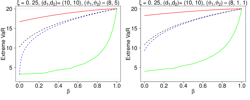
Figure 4: Upper and lower bounds on extreme VaR for a composite market plus sectors portfolio. The dashed lines indicate the closed-form expressions based on (4.7). The solid lines indicate the conservative bounds based on a single $d$-variate extremal coefficient constraint without any structural assumptions.

Figure 4 illustrates the significant reduction in the range of possible extreme VaR values based on the above setup for a range of $\beta$-values. We have the simple partition into $k=2$ sectors and $(d_{1},d_{2})=(10,10)$. Considered are two cases where the within-sector $d_{i}$-variate extremal coefficients in (4.6) are $(\vartheta_{\mathbf{X}(1)}(J_{1}),\vartheta_{\mathbf{X}(2)}(J_{2}))=(8,5)$ (left panel) and $(\vartheta_{\mathbf{X}(1)}(J_{1}),\vartheta_{\mathbf{X}(2)}(J_{2}))=(8,1.1)$ (right panel). In both cases $\xi=0.25$. The dotted horizontal lines indicate the Hoeffding-Fréchet bounds on extreme VaR. The solid green and red lines correspond to the exact lower/upper bounds obtained by imposing a single $d$-variate constraint with

$$\vartheta_{\mathbf{X}}(\{1,\dots,d\})=\beta+(1-\beta)\times\sum_{i=1}^{k}\vartheta_{\mathbf{X}(i)}(J_{i}).$$

Finally, the dashed blue/black lines correspond to the lower/upper bounds for $\rho$ obtained by using the decomposition into a single market factor effect plus independent sector-specific risks. Observe the significant reduction in the range of possible values for extreme VaR. This is naturally attributed to the assumption of independence among the sectors. The presence of a single asymptotically completely dependent market factor, however, can make this range approach the ultimate upper bound for $\beta\to 1$. Alternatively, if the proportion of the market risk is low ($\beta\to 0$), the lower bound approaches the ultimate single d-variate constraint lower bound (solid green curve) in the left panel. In the right panel, however, one observes a non-trivial gap between the two lower bounds at $\beta=0$. This can be attributed to the fact that the constraint $\vartheta_{\mathbf{X}(2)}(J_{2})=1.1$ is rather close to complete dependence for the second sector, while the overall portfolio constraint on $\vartheta_{\mathbf{X}}(\{1,\dots,d\})$ is far from complete dependence. Thus, the additional sector-specific information leads to far less optimistic lower bound on extreme VaR than in the market-structure-agnostic case.

The proportion of market-wide risk $\beta$ here was assumed to be known, for illustration purposes. Using (4.5), however, $\beta$ can be readily estimated in practice from an extremal coefficient $\vartheta_{\mathbf{X}}(J)$ involving a set $J$ of two or more sectors. For example, given $\vartheta_{\mathbf{X}}(\{1,\dots,d\})=c_{0}(\mathbf{X})$ and $\vartheta_{\mathbf{X}}(J_{i})=c_{i}(\mathbf{X}),\ i=1,\dots,k$, we obtain

$$c_{0}(\mathbf{X})=\beta+(1-\beta)\times\sum_{i=1}^{k}\vartheta_{\mathbf{X}(i)}(J_{i})\quad\mbox{ and }\ c_{i}(\mathbf{X})=\beta+(1-\beta)\times\vartheta_{\mathbf{X}(i)}(J_{i}),\ i=1,\dots,k.$$

By elimination, these linear equations yield

$$\beta=\frac{\Big{(}\sum_{i=1}^{k}(c_{i}(\mathbf{X})\Big{)}-c_{0}(\mathbf{X})}{k-1},\ \ \mbox{ as well as }\ \ \vartheta_{\mathbf{X}(i)}(J_{i})=\frac{c_{i}(\mathbf{X})-\beta}{1-\beta}.$$

5 Summary and discussion

Under the general assumption of multivariate regular variation, the extreme Value-at-Risk of a $d$-dimensional portfolio, relative to a baseline asset, can be expressed as an integral functional with respect to a finite measure on the unit simplex. This, unknown (spectral) measure, is an infinite-dimensional parameter that encodes the complete extremal (joint) dependence structure of the assets in the portfolio. In practice, the conventional estimation of the spectral measure is challenging or impossible. This motivated us to adopt distributionally robust perspective. Namely, study the optimization problems of finding the infimum and supremum of the extreme VaR functional over large classes of possible spectral measures. Using popular and interpretable extremal coefficient constraints, we expressed the above optimization problems as duals to linear semi-infinite programs, which in turn were shown to have no duality gap. Thus, a number of results on the structure of spectral measures corresponding to the best- and worst-case extreme VaR were obtained. In the special case of scale balanced portfolia, we have also shown that the lower bound on extreme VaR corresponds to a spectral measure of the so-called Tawn-Molchanov multivariate max-stable model, which can be solved with conventional linear programs. We have also established surprising closed-form expressions for the lower- and upper-bound on extreme VaR under single $d$-variate extremal coefficient constraints, valid in all dimensions $d$. These results were further illustrated and extended in the case of the market-and-sectors framework. The theoretical results were shown to provide practical bounds in a limited real data example, and compared with conventional extreme value theory method.

Our contributions are mostly theoretical. However, the established results, formulae and methods are motivated by important challenges in quantifying model uncertainty when studying the risk of extremes in high-dimensional portfolia. To provide a complete practical methodology for risk assessment a number of implortant problems remain to be addressed. Namely,

• Develop practical or approximate solvers for the optimization problems in dimensions $d>10$.

• Study the optimal set of constraints ${\cal J}$ in terms of greatest reduction of the range of possible extreme VaR.

• Quantify the uncertainty in the resulting lower- and upper-bounds on extreme VaR stemming from the statistical error in the estimation of the tail index $\xi$ and extremal coefficient constraints.

Finally, one very important open problem that stands out in our opinion is to establish closed form formulae in the case of single $d$-variate constraints (as in Theorems 3.7 and 3.8) for a general un-balanced portfolio. Such formulae, by the method of partitioning, can lead to significant improvements on the range of extreme VaR similar to the ones obtained in Section 4.2.

Appendix A Multivariate regular variation and extremes

For convenience of the reader, here we review some facts and technical results on multivariate regular variation and extremes. For more details, see the comprehensive monographs [26, 9, 27] and the recent general approach to regular variation in metric spaces [19]. Some applications and extensions can be found in [21] and [31].

Definition A.1.

A random vector $\mathbf{X}=(X_{i})_{i=1}^{d}$ in $\mathbb{R}^{d}$ is said to be multivariate regularly varying (MRV), if there exist a sequence $a_{n}\geq 0,\ a_{n}\uparrow\infty$ and a Borel measure $\mu$ on $\mathbb{R}^{d}\setminus\{\mathbf{0}\}$, such that:

(i) $\mu(A)<\infty$, for all Borel sets $A$, bounded away from the origin, i.e., such that $A\subset\mathbb{R}^{d}\setminus B(\mathbf{0},\epsilon),$ for some $\epsilon>0$, where $B(\mathbf{0},\epsilon)$ denotes a ball centered at $\mathbf{0}$ with radius $\epsilon$.

(ii) For all Borel sets $A$, bounded away from $\mathbf{0}$ and such that $\mu(\partial A)=0$, we have

$$n\mathbb{P}(a_{n}^{-1}\mathbf{X}\in A)\longrightarrow\mu(A),\ \ \mbox{ as }n\to\infty.$$ (A.1)

In this case, we write $\mathbf{X}\in RV(\{a_{n}\},\mu)$.

It can be shown that if $\mathbf{X}\in RV(\{a_{n}\},\mu)$, the sequence $a_{n}$ is necessarily regularly varying, i.e. there exist a positive constant $\xi>0$, such that $a_{[tn]}/a_{n}\to t^{\xi},$ as $n\to\infty$, for all $t>0$. Furthermore, the limit measure $\mu$ has the scaling property $\mu(cA)=c^{-1/\xi}\mu(A)$, for all $c>0$. Different choices for the normalization sequence $\{a_{n}\}$ are possible, however, the exponent $\xi$ is uniquely defined, given a random vector $\mathbf{X}$. To indicate that, we sometimes write $\mathbf{X}\in RV_{1/\xi}(\{a_{n}\},\mu)$.

An alternative, equivalent approach to multivariate regular variation is through polar coordinates. Namely, let $\|\cdot\|$ be an arbitrary norm in $\mathbb{R}^{d}$ (In fact, one can consider any positive and $1$-homogeneous continuous function on $\mathbb{R}^{d}\setminus\{\mathbf{0}\}$ as the radial component see, e.g., [31].) Then, $\mathbf{X}\in RV(\{a_{n}\},\mu)$, if and only if, for any (all) $s>0$,

$$n\mathbb{P}(a_{n}^{-1}\|\mathbf{X}\|>s,\ \mathbf{X}/\|\mathbf{X}\|\in\cdot)\stackrel{{\scriptstyle w}}{{\longrightarrow}}cs^{-1/\xi}\sigma(\cdot),\ \ \mbox{ as }n\to\infty,$$ (A.2)

for some probability measure $\sigma$ defined on the unit sphere ${\mathbb{S}}_{\|\cdot\|}:=\{\mathbf{x}\,:\,\|\mathbf{x}\|=1\}$. It can be easily seen from (A.1) and (A.2), by setting $s=1$, that

$$c=\mu(\{\|\mathbf{x}\|>1\})\ \ \mbox{ and, in fact, }\ \ \sigma(B)=\frac{\mu(\{\|\mathbf{x}\|>1,\mathbf{x}/\|\mathbf{x}\|\in B\})}{\mu(\{\|\mathbf{x}\|>1\})}.$$

for a Borel set $B\subset{\mathbb{S}}_{\|\cdot\|}.$ Relation (A.2) can be interpreted in terms of polar coordinates as follows. Letting $\mathbf{X}\rightsquigarrow(R,\mathbf{U})$ with $R:=\|\mathbf{X}\|$ and $\mathbf{U}:=\mathbf{X}/\|\mathbf{X}\|$, we have that

$$n\mathbb{P}(a_{n}^{-1}R>s)\to cs^{-1/\xi}\ \ \mbox{ and }\ \ \mathbb{P}(\mathbf{U}\in\cdot|R>a_{n})\stackrel{{\scriptstyle w}}{{\longrightarrow}}\sigma(\cdot),$$

as $n\to\infty$. This means, that the vector $\mathbf{X}\rightsquigarrow(R,\mathbf{U})$ is MRV if and only if its radial component is regularly varying and the conditional distribution of its angular component, given that the radius is extreme, converges weakly to the probability measure $\sigma$ (see, e.g., [19] and Prop 3.9 in [31]). The probability measure $\sigma$ is referred to as the spectral measure of $\mathbf{X}$. Observe that, depending on the choice of the normalizing sequence $\{a_{n}\}$, the measure $\mu$ in (A.1) and correspondingly, the constant $c$ in (A.2), may change. The spectral measure $\sigma$ and the exponent $1/\xi$, however, are uniquely defined, given a RV vector $\mathbf{X}$.

The measure $\mu$ has the polar coordinate representation $\mu(d\mathbf{x})=c\nu_{1/\xi}(dr)\sigma(d\mathbf{u})$, where is $\nu_{1/\xi}$ is a measure on $(0,\infty)$, such that $\nu_{1/\xi}(c,\infty)=c^{-1/\xi},\ c>0$. More precisely, we have the disintegration formula:

$$\mu(A)=c\int_{\mathbb{S}_{\|\cdot\|}}\int_{0}^{\infty}1_{A}(r\mathbf{u})(1/\xi)r^{-1-1/\xi}dr\sigma(d\mathbf{u}).$$ (A.3)

A.1 Multivariate extremes

In the context of extreme value theory, the spectral measure $\sigma$ can be used to express the cumulative distribution function of the asymptotic distribution of independent component-wise maxima. Specifically, let $\mathbf{X}=(X_{i})_{i=1}^{d},\ \mathbf{X}(k),\ k=1,\ldots,n$ be iid RV$(\{a_{n}\},\mu)$. For simplicity, assume that the $X_{i}$’s are non-negative. Then, the measure $\mu$ concentrates on $[0,\infty)^{d}\setminus\{\mathbf{0}\}$. Consider the component-wise maxima $M_{i}(n):=\max_{k=1,\ldots,n}X_{i}(k),\ i=1,\ldots,d$. Then, it can be shown that for all $\mathbf{x}=(x_{i})_{i=1}^{d}\in[0,\infty)^{d}\setminus\{\mathbf{0}\}$,

$$\mathbb{P}{\Big{(}}a_{n}^{-1}M_{i}(n)\leq x_{i},\ i=1,\ldots,d{\Big{)}}\longrightarrow G_{\mu}(\mathbf{x}):=\exp{\Big{\{}}-\mu([\mathbf{0},\mathbf{x}]^{c}){\Big{\}}},\ \ \mbox{ as }n\to\infty.$$ (A.4)

That is, $a_{n}^{-1}\mathbf{M}_{n}:=a_{n}^{-1}(M_{i}(n))_{i=1}^{d}$ converges in distribution to a vector $\mathbf{Y}$ with the cumulative distribution function $G_{\mu}$ given above. Indeed, by the independence of the $\mathbf{X}(k)$’s, we have

$$\mathbb{P}{\Big{(}}a_{n}^{-1}\mathbf{M}(n)\leq\mathbf{x}{\Big{)}}=\mathbb{P}{\Big{(}}a_{n}^{-1}\mathbf{X}\leq\mathbf{x}{\Big{)}}^{n}={\Big{(}}1-\frac{n\mathbb{P}(a_{n}^{-1}\mathbf{X}\in A)}{n}{\Big{)}}^{n},$$ (A.5)

where $A=[\mathbf{0},\mathbf{x}]^{c}$, $\mathbf{M}(n)=(M_{i}(n))_{i=1}^{d}$ and the above inequalities are considered component-wise. By using the scaling property of $\mu$, it can be shown that $A$ is a continuity set, and hence (A.1) implies that $n\mathbb{P}(a_{n}^{-1}\mathbf{X}\in A)\to\mu(A)$, as $n\to\infty$. Hence, the right-hand side of (A.5) converges to $\exp\{-\mu(A)\}$, which is in fact the right-hand side of (A.4).

Consider now the disintegration formula (A.3) with $A=[\mathbf{0},\mathbf{x}]^{c}$. Notice that $r\mathbf{u}\in A$ if $ru_{i}>x_{i}$, for some $i=1,\ldots,d$, or equivalently $r>\min_{i=1,\ldots,d}x_{i}/u_{i}$. Therefore, by (A.3), we have

$$\mu(A)=c\int_{\mathbb{S}_{\|\cdot\|}}\int_{\min_{i=1,\ldots,d}x_{i}/u_{i}}(1/\xi)r^{-1-1/\xi}dr\sigma(d\mathbf{u})=c\int_{\mathbb{S}_{\|\cdot\|}}{\Big{(}}\max_{i=1,\ldots,d}{u_{i}\over x_{i}}{\Big{)}}^{1/\xi}\sigma(d\mathbf{u}).$$

That is, we obtain the following well-known expression of the distribution function $G_{\mu}$:

$$\mathbb{P}(\mathbf{Y}\leq\mathbf{x})\equiv G_{\mu}(\mathbf{x})=\exp{\Big{\{}}-c\int_{\mathbb{S}_{\|\cdot\|}}{\Big{(}}\max_{i=1,\ldots,d}{u_{i}\over x_{i}}{\Big{)}}^{1/\xi}\sigma(d\mathbf{u}){\Big{\}}},$$ (A.6)

$\mathbf{x}\in\mathbb{R}_{+}^{d}\setminus\{\mathbf{0}\}$ (see, e.g., Ch. 5 in [26]).

A.2 Extremal coefficients

Let $J\subset\{1,\ldots,d\}$ be a non-empty subset of coordinates of the random vector $\mathbf{Y}$ in (A.6). Recall that the extremal coefficient ${\vartheta}(J)$ is defined as follows

$$\mathbb{P}{\Big{(}}\max_{j\in J}Y_{j}\leq 1{\Big{)}}=:\exp\{-{\vartheta}(J)\}.$$

In view of (A.6), we have

$${\vartheta}(J)=c\int_{\mathbb{S}_{\|\cdot\|}}{\Big{(}}\max_{j\in J}u_{i}^{1/\xi}{\Big{)}}\sigma(d\mathbf{u}).$$ (A.7)

Moreover, by (A.4) one can show that

$$n\mathbb{P}{\Big{(}}\max_{j\in J}X_{j}>a_{n}x{\Big{)}}\longrightarrow{\vartheta}(J),\ \mbox{ as }n\to\infty.$$

Therefore, modulo a common scaling factor, all these extremal coefficients can be readily estimated via the asymptotic scale coefficients of the heavy-tailed distributions $\max_{j\in J}X_{j}$. Specifically, we have

$$\lim_{x\to\infty}\frac{\mathbb{P}(\max_{j\in J}X_{j}>x)}{\mathbb{P}(X_{1}>x)}={{\vartheta}(J)\over{\vartheta}(\{1\})},\ \ J\subset\{1,\ldots,d\}.$$

By suitable rescaling of the reference asset $X_{1}$ (or equivalently, the normalization sequence $\{a_{n}\}$), without loss of generality, we may assume that $\vartheta(\{1\})=1.$ Given independent copies $\mathbf{X}_{i},\ i=1,\ldots,n$ of $\mathbf{X}$, define the self-normalized estimators

$$\widehat{\vartheta}_{x}(J):={\sum_{i=1}^{n}\mathbb{I}(\max_{j\in J}X_{j}(i)>x)\over\sum_{i=1}^{n}\mathbb{I}(X_{1}(i)>x)}.$$ (A.8)

Remark A.2.

It can be shown that the estimators in (A.8) are weakly consistent for any choice of a regularly varying sequence $x=x_{n}\to\infty$ such that $n\mathbb{P}(X_{1}(i)>x_{n})\to\infty$, as $n\to\infty$, i.e., we have $\hat{\vartheta}_{x_{n}}(J)\to\vartheta(J)$ in probability. This is true for example for the sequence $x_{n}:=n^{1/(1/\xi+\delta)},$ for any $\delta>0$. The consistency of $\hat{\vartheta}_{x_{n}}(J)$ follows by applying Theorem 5.3.(ii) in [27] to both the numerator and denominator in (A.8), viewed as empirical measures of the type $b_{n}^{-1}\sum_{i=1}^{n}{\mathbb{I}}_{\{Y(i)/x_{n}\}}(\cdot)$, where $Y(i)$ stands for either $X_{1}(i)$ or $\max_{j\in J}X_{j}(i)$. The sequence $b_{n}\nearrow\infty$ herein is chosen such that $(n/b_{n})\mathbb{P}(X_{1}(i)>x_{n}s)\to s^{-1/\xi},$ as $n\to\infty$, for all $s>0$. The fact that such a sequence $b_{n}$ can be found follows from the regular variation property of $x_{n}$ and the distribution of $X_{1}(i)$.

Remark A.3.

Recall Remark 2.1. The empirically estimated extremal coefficients in (A.8) do satisfy the consistency relationships of a set of valid extremal coefficients. Indeed, it follows from Lemma A.5 (below), with $x_{j}:=\mathbb{I}(X_{j}(i)>x)$ that

$$\sum_{L\,:\,J\subseteq L\subseteq\{1,\dots,d\}}(-1)^{|L\setminus J|+1}\max_{j\in L}\mathbb{I}\Big{(}X_{j}(i)>x\Big{)}\equiv\sum_{L\,:\,J\subseteq L\subseteq\{1,\dots,d\}}(-1)^{|L\setminus J|+1}\mathbb{I}\Big{(}\max_{j\in L}X_{j}(i)>x\Big{)}\geq 0,$$

for all $i$. Thus, the desired consistency relationships in Remark 2.1, follow by summing over $i$ since the denominator in (A.8) is common and positive.

Remark A.4.

In practice, however, when the extremal coefficients are either imposed or estimated in some other way, different from (A.8), one needs to ensure they provide consistent constraints. This can be done by “projecting” them onto the convex set of valid vectors of extremal coefficients ${\bf c}_{\cal J}=(c_{J})_{J\in{\cal J}}$. Specifically, by Möbius inversion, we know that ${\bf c}_{\cal J}=A\boldsymbol{\beta}$, where $\boldsymbol{\beta}\in\mathbb{R}_{+}^{2^{d}-1}$ and a certain design matrix $A$ of dimension $|{\cal J}|\times(2^{d}-1)$. In practice, if the vector of estimated coefficients is $\widehat{\bf c}_{\cal J}$, we solve the quadratic optimization program

$${\rm minimize}\ \Big{\{}\|\widehat{\bf c}_{\cal J}-A{\boldsymbol{\beta}}\|^{2}+\lambda\|\boldsymbol{\beta}\|^{2}\Big{\}},$$

subject to $\boldsymbol{\beta}\geq{\bf 0}$, for some small regularization parameter $\lambda>0$. We take the solution $A\boldsymbol{\beta}$ as the constraints in our extreme VaR optimization algorithms. In our experience, the so-calibrated extremal coefficient constraints are quite close to the ones estimated in practice. This calibration and other important statistical issues merit further independent investigation.

The following elementary lemma follows by induction, although it may be possible to obtain with general Möbius inversion techniques. This result is used to show that the empirical extremal coefficients in (A.8) satisfy the consistency relationships of a valid set of extremal coefficients (cf Remark 2.1).

Lemma A.5.

Let $d\geq 2$ be an integer. For all $x_{i}\geq 0,\ i=1,\dots,d$, and $J\subset\{1,\dots,d\},\ J\not=\{1,\dots,d\}$, we have

$$S(J):=\sum_{L\,:\,J\subseteq L\subseteq\{1,\dots,d\}}(-1)^{|L\setminus J|+1}x_{j}\geq 0,$$

where by convention $\max_{j\in\emptyset}x_{j}:=0$.

Proof.

We establish the claim by induction. If $J=\{1,\dots,d\}\setminus\{j_{0}\}$, then trivially $S(J)=0$, if $\max_{j\in J}x_{j}\geq x_{j_{0}}$ and $S(J)=x_{j_{0}}-\max_{j\in J}x_{j}>0$, otherwise. This proves that $S(J)\geq 0$, for all $J$ such that $|J|=d-1$.

Suppose, now that $|J|\leq d-2$ and $S(\widetilde{J})\geq 0$, for all $|\widetilde{J}|\geq|J|+1$. Let $\{j_{1},\dots,j_{m}\}:=\{1,\dots,d\}\setminus J$ and observe that

$$S(J)=-\max_{j\in J}x_{j}+\sum_{i=1}^{m}\max_{j\in J\cup\{j_{i}\}}x_{j}+\sum_{i=1}^{m}S(J\cup\{j_{i}\}).$$

The latter however is non-negative. Indeed, by the induction assumption, we have $S(J\cup\{j_{i}\})\geq 0$, while $\max_{j\in J\cup\{j_{i}\}}\geq\max_{j\in J}x_{j}$, for each $i=1,\dots,m$, which since the $x_{j}$’s are non-negative implies that $S(J)\geq 0$. Appealing to the induction principle, we conclude the proof. ∎

A.3 On Extreme VaR for homogeneous risk functionals

Let $\mathbf{X}\in RV_{1/\xi}(\{a_{n}\},\mu)$ be a vector of losses. It is convenient to write $\mathbf{X}=(Z_{i}^{\xi})_{i=1}^{d}$, where $\mathbf{Z}=(Z_{i})_{i=1}^{d}\in RV_{1}(\{b_{n}\},\nu)$, with $b_{n}:=a_{n}^{1/\xi}$ and $\nu(A)=\mu(A^{\xi})$.

Consider a set of positive portfolio weights $w_{i}>0,\ i=1,\ldots,d$ for the $d$ assets. Then, the cumulative portfolio loss $S=\sum_{i=1}^{d}w_{i}X_{i}$ can be expressed as

$$S=h_{\mathbf{w}}(\mathbf{Z}),\ \ \mbox{ where }\ h(\mathbf{z})=\sum_{i=1}^{d}w_{i}z_{i}^{\xi}\equiv\sum_{i=1}^{d}w_{i}z_{i}^{\xi},$$

is a positive, $\xi$-homogeneous function of $\mathbf{Z}$.

The asymptotic scale of the loss $S$ relative to a reference asset is the key ingredient in computing extreme Value-at-Risk. Indeed, if

$$\rho:=\lim_{x\to\infty}\frac{\mathbb{P}(S>x)}{\mathbb{P}(X_{1}>x)},$$ (A.9)

then by Lemma 2.3 in [12], we have that

$$\lim_{q\nearrow 1}\frac{VaR_{q}(S)}{VaR_{q}(X_{1})}=\rho^{\xi}.$$ (A.10)

The following result is extends the formulae in [3] (see also Theorem 4.1 of [12]), which address only the case of equal portfolio weights and tail-equivalent losses.

Proposition A.6.

Let $\mathbf{Z}=(Z_{i})_{i=1}^{d}:=(X_{i}^{1/\xi})_{i=1}^{d}\in RV_{1}(\{b_{n}\},\nu)$ be a non-negative regularly varying random vector with exponent equal to $1$. Fix a norm $\|\cdot\|$ in $\mathbb{R}^{d}$ and let $\sigma_{\mathbf{Z}}$ be the spectral measure of $\mathbf{Z}$ induced on the positive unit sphere $\mathbb{S}_{\|\cdot\|}^{+}:=\{\mathbf{x}\geq\mathbf{0}\,:\,\|\mathbf{x}\|=1\}$. That is,

$$\nu(d\mathbf{x})=cr^{-2}dr\sigma_{\mathbf{Z}}(d\mathbf{u}),$$ (A.11)

where $c=\nu\{\|\mathbf{x}\|>1\}$ and $(r,u):=(\|\mathbf{x}\|,\mathbf{x}/\|\mathbf{x}\|)$ are the polar coordinates in $[0,\infty)^{d}\setminus\{\mathbf{0}\}$.

For $\rho_{\mathbf{w}}=\rho(S,X_{1})$ in (A.9), we have

$$\rho_{\mathbf{w}}(S,X_{1})=\frac{1}{\sigma_{1}}\int_{S_{\|\cdot\|}^{+}}{\Big{(}}\sum_{i=1}^{d}w_{i}u_{i}^{\xi}{\Big{)}}^{1/\xi}\sigma_{\mathbf{Z}}(d\mathbf{u}),$$ (A.12)

where $\sigma_{1}:=\int_{S_{\|\cdot\|}^{+}}u_{1}\sigma_{\mathbf{Z}}(d\mathbf{u})$.

The proof is a direct consequence of the next lemma, which establishes the asymptotic scale of $h(\mathbf{Z})$ for a general $\xi$-homogeneous risk functional $h$.

Lemma A.7.

Let $\mathbf{Z}$ be as in Proposition A.6 and $h:[0,\infty)^{d}\to[0,\infty)$ be an arbitrary non-negative $\xi-$homogeneous function, i.e. $h(c\mathbf{x})=c^{\xi}h(\mathbf{x}),\ \forall c>0$. Then, for all $s>0$, we have

$$n\mathbb{P}(b_{n}^{-1/\xi}h(\mathbf{Z})>s)\longrightarrow c\times\rho(h)s^{-1/\xi},\ \ \mbox{ as }n\to\infty,$$

where

$$\rho(h)=\int_{\mathbb{S}_{\|\cdot\|}^{+}}h(\mathbf{u})^{1/\xi}\sigma_{\mathbf{Z}}(d\mathbf{u}).$$ (A.13)

This result shows that $h(\mathbf{Z})$ is regularly varying (provided $\rho(h)>0$) and in fact it identifies its asymptotic scale coefficient in terms of the spectral measure $H$.

Proof of Lemma A.7.

By Theorem 6 and Remark 7 of [18], we have that

$$n\mathbb{P}(h(b_{n}^{-1}\mathbf{Z})>s)\longrightarrow\nu\circ h^{-1}(s,\infty),\ \ \mbox{ as }n\to\infty.$$ (A.14)

Note that the above convergence is valid for all $s>0$ since the by the scaling property of $\nu$ and the homogeneity of $h$, all sets $h^{-1}(s,\infty)=s^{1/\xi}h^{-1}(1,\infty)$ are in fact continuity sets of $\nu$. It remains to express the right-hand side of (A.14) in terms of the spectral measure $\sigma_{\mathbf{Z}}$. In view of (A.11) and by using the $\xi$-homogeneity of $h$, we obtain

$$\nu\circ h^{-1}(s,\infty) = c\int_{\mathbb{S}_{\|\cdot\|}^{+}}\int_{0}^{\infty}1_{h^{-1}(s,\infty)}(r\mathbf{u})r^{-2}dr\sigma_{\mathbf{Z}}(d\mathbf{u})$$

$$= c\int_{\mathbb{S}_{\|\cdot\|}^{+}}\int_{0}^{\infty}1_{(s,\infty)}(r^{\xi}h(\mathbf{u}))r^{-2}dr\sigma_{\mathbf{Z}}(d\mathbf{u})$$

$$= c\int_{\mathbb{S}_{\|\cdot\|}^{+}}\int_{0}^{\infty}1_{((s/h(\mathbf{u}))^{1/\xi},\infty)}(r)r^{-2}dr\sigma_{\mathbf{Z}}(d\mathbf{u})$$

$$= c\int_{\mathbb{S}_{\|\cdot\|}^{+}}(s/h(\mathbf{u}))^{-1/\xi}\sigma_{\mathbf{Z}}(d\mathbf{u}).$$

The last expression equals $c\rho(h)s^{-1/\xi}$, where $\rho(h)$ is given in (A.13). ∎

Remark A.8.

By using Lemma 2.3 of [12] and our Lemma A.7, one can establish the asymptotic value-at-risk for more complicated instruments, which are non-linear homogeneous functions of the underlying assets. For example, one can consider $h(\mathbf{u}):=\min_{i=1,\ldots,d}u_{i}^{\xi}$. Thus, $h(\mathbf{Z})=\min_{i=1,\ldots,d}X_{i}$ represents the minimum loss of a portfolio and bounds on its extreme VaR may be of interest. Note that in this case

$$\lim_{x\to\infty}\frac{\mathbb{P}(\min_{i=1,\ldots,d}X_{i}>x)}{\mathbb{P}(X_{1}>x)}=\frac{1}{\sigma_{1}}\int_{S_{\|\cdot\|}^{+}}{\Big{(}}\min_{i=1,\ldots,d}u_{i}{\Big{)}}\sigma_{\mathbf{Z}}(d\mathbf{u})$$

does not depend on $\xi$.

A.4 On the role of the tail index in risk diversification

Here, we briefly comment on an intriguing phase transition in the Fréchet-type bounds for the coefficient $\rho_{\mathbf{w}}$ in (1.9) occurring in the case when $\xi>1$. Recall that extreme VaR equals $\rho_{\mathbf{w}}^{\xi}$, where $1/\xi$ is the tail exponent of the portfolio $\mathbf{X}$.

The case $0<\xi<1$ corresponds to a finite-mean model for the losses. In the case $\xi>1$, we have an infinite mean model, which may be viewed as ‘catastrophic’ since one has to have infinite capital in order to guard against such losses in the long-run. The bounds on $\rho_{\mathbf{w}}$ can be interpreted as follows:

• In the light-tailed case $0<\xi<1$ the means of the losses are finite and then the lower bound $\rho_{\mathbf{w}}=\sum_{i=1}^{d}w_{i}$ is achieved by the asymptotically independent portfolio. This agrees with the general intuition that accumulating independent assets leads to diversification and lower risk. On the other hand, the worst case scenario, naturally, corresponds to perfect (asymptotic) dependence where all assets are asymptotically identical or no diversification at all.

• In the boundary case $\xi=1$, the two bounds coincide, regardless of the asymptotic portfolio dependence.

• In the extreme heavy-tailed setting $\xi>1$ the means of the losses are infinite and it turns out that the bounds in (1.9) are reversed. Indeed, by the triangle inequality, for the $L^{\xi}-$norm, we obtain:

  $$\rho_{\mathbf{w}} =\int_{\mathbb{S}_{+}}\Big{(}w_{1}u_{1}^{\xi}+\cdots+w_{d}u_{d}^{\xi}\Big{)}^{1/\xi}H(d\mathbf{u})\leq\sum_{i=1}^{d}w_{i}^{1/\xi}\int_{\mathbb{S}_{+}}u_{i}H(d\mathbf{u})=\sum_{i=1}^{d}w_{i}^{1/\xi},$$

  where in the last relation we used the moment constraints in (1.8). Thus, the expression for the lower bound in the case $0<\xi<1$ in (1.9) now, in the case $\xi>1$, becomes the upper bound.

  On the other hand, by the Jensen’s inequality, for the concave function $x\mapsto x^{1/\xi}$, we have

  $$\left(w_{1}u_{1}^{\xi}+\cdots+w_{d}u_{d}^{\xi}\right)^{1/\xi}\geq\Big{(}\sum_{i=1}^{d}w_{i}\Big{)}^{1/\xi}\sum_{i=1}^{d}\widetilde{w}_{i}u_{i},$$

  where $\widetilde{w}_{i}:=w_{i}/(\sum_{j=1}^{d}w_{j})$, so that $\sum_{i=1}^{d}\widetilde{w}_{i}=1$. By integrating the last bound with respect to $H(d\mathbf{u})$, and using the moment constraints (1.8), we obtain

  $$\rho_{\mathbf{w}}\equiv\int_{\mathbb{S}_{+}}\left(w_{1}u_{1}^{\xi}+\cdots+w_{d}u_{d}^{\xi}\right)^{1/\xi}H(d\mathbf{u})\geq\Big{(}\sum_{i=1}^{d}w_{i}\Big{)}^{1/\xi}.$$

  This shows that the expression for the upper bound in (1.9) (for the case $0<\xi<1$) now (in the case $\xi>1$) yields the lower bound.

  In summary, for the case $\xi>1$, we obtain the following universal bounds on $\rho_{\mathbf{w}}$ (see also (1.9))

  $$\Big{(}\sum_{i=1}^{d}w_{i}\Big{)}^{1/\xi}\leq\rho_{\mathbf{w}}\leq\sum_{i=1}^{d}w_{i}^{1/\xi}.$$

  The bounds are sharp. The upper bound corresponds to asymptotic independence, and the lower to complete (asymptotic) dependence. This contradicts with our intuition about diversification. It shows that in the infinite-mean scenario, of potentially catastrophic losses, it is best to just hold a single asset rather than to ‘diversify’ among independent ones. The following argument provides some explanation of this counter-intuitive phenomenon.

  Let $X_{i},\ i=1,2,\ldots,$ be non-negative independent and identically distributed random variables modeling losses. Suppose that $\mathbb{P}(X_{i}>x)\sim cx^{-1/\xi},\ x\to\infty,\ c>0$, with $\xi>1$ so that we are in the extreme heavy tailed regime of infinite expected loss $\mathbb{E}(X_{i})=\infty$. Suppose that unit investment is distributed evenly among $n$ such potentially catastrophic assets resulting in a portfolio loss

  $$S_{n}:=\frac{1}{n}\sum_{i=1}^{n}X_{i}.$$

  Then, by the heavy-tailed version of the central limit theorem, we have

  $$\frac{1}{n^{\xi}}\sum_{i=1}^{n}X_{i}=\frac{S_{n}}{n^{\xi-1}}\stackrel{{\scriptstyle d}}{{\longrightarrow}}Z,\ \ \mbox{ as }n\to\infty,$$

  where $Z$ is a non-trivial totally skewed, $(1/\xi)$-stable random variable [30]. In this case, since $(\xi-1)>0$, the total loss $S_{n}\stackrel{{\scriptstyle d}}{{\approx}}n^{\xi-1}Z$ stochastically grows to infinity as the number of independent assets in the portfolio increases. This counter-intuitive phenomenon where distributing an investment among multiple independent assets is in fact detrimental is due the extreme heavy-tailed nature of the model. Although such catastrophic models may not be practically relevant, the above argument shows that during regimes of very extreme losses our intuition about diversification may fail.

Appendix B Proofs

B.1 Karush–Kuhn–Tucker Conditions

The following proposition establishes sufficient conditions for optimal solutions to an LSIP $(P)$. This version of the classic Karush–Kuhn–Tucker (KKT) optimality conditions for the case of LSIPs will be used in the proofs for Theorems 3.4, 3.7 and 3.8.

Proposition B.1 (KKT conditions).

Suppose Assumption 2.3 is satisfied and $\mathrm{val}(P)<\infty$. Fix $\boldsymbol{x}\in\mathbb{R}^{p}$. If there exists dual variables $(y_{1},y_{2},\ldots,y_{p})^{\top}\in\mathbb{R}_{+}^{p}$ and $\{t_{1},\ldots,t_{p}\}\subset T$ such that

$$\sum_{k=1}^{p}y_{k}\boldsymbol{a}(t_{k})=\boldsymbol{c},$$ (B.1)

$$\boldsymbol{a}(t_{k})^{\top}\boldsymbol{x}=b(t_{k}),\ k=1,\ldots,p,$$ (B.2)

and

$$\boldsymbol{a}(t)^{\top}\boldsymbol{x}\geq b(t),\ \text{for all }t\in T.$$ (B.3)

Then $\boldsymbol{x}\in\mathrm{sol}(P)$.

Proof.

For every $\boldsymbol{x}\in\mathbb{R}^{p}$, define the set of active indices $T(\boldsymbol{x}):=\{t\in T:\boldsymbol{a}(t)^{\top}\boldsymbol{x}=b(t)\}.$ By Theorem 7.1.(ii) of [16] (see also Section 11.2 therein), a primal feasible vector $\tilde{\boldsymbol{x}}\in\mathbb{R}^{p}$ is optimal for $(P)$ whenever

$$\boldsymbol{c}\in\mathrm{cone}\left\{\boldsymbol{a}(t):t\in T(\tilde{\boldsymbol{x}})\right\},$$ (B.4)

where $\mathrm{cone}\{C\}$ denotes the smallest convex cone containing $C\subset\mathbb{R}^{p}$. This is true in our setting. Indeed, Relation (B.2) implies that $\{t_{1},\dots,t_{p}\}\subset T(\boldsymbol{x})$, which in view of (B.1) entails (B.4). ∎

B.2 Proof for the Tawn-Molchanov minimizer

In this section, let $D=\{1,\ldots,d\}$. Denote $2^{D}$ as the power set of $D$ and $K^{c}=D\backslash K.$ We shall need two auxiliary lemmas.

Lemma B.2.

Let $0\leq u_{(1)}\leq u_{(2)}\leq\cdots\leq u_{(d)}\leq 1$ be the order statistics for arbitrary $\boldsymbol{u}\in\mathbb{S}_{+}^{d-1}$Fix $\xi>0$ and define $u_{(0)}=0$. The following equality holds

$$\sum_{J\in 2^{D}\backslash\varnothing}\max_{j\in J}\{u_{j}\}\sum_{L\subset J}(-1)^{|L|+1}|J^{c}\cup L|^{1/\xi}=\sum_{j=1}^{d}(d+1-j)^{1/\xi}\left(u_{(j)}-u_{(j-1)}\right).$$ (B.5)

Proof.

We will prove (B.5) under the assumption that there are no ties, i.e., $u_{(1)}<u_{(2)}\cdots<u_{(d)}$. Since both the left- and right-hand sides of (B.5) are continuous functions of the $u_{i}$’s, the general result will follow by continuity for all $\mathbf{u}\in\mathbb{S}_{+}^{d-1}$.

We have

$$\sum_{J\in 2^{D}\backslash\varnothing}\max_{j\in J}\{u_{j}\}\sum_{L\subset J}(-1)^{|L|+1}|J^{c}\cup L|^{1/\xi}$$

$$\quad\quad\quad=\sum_{i=1}^{d}u_{(i)}\left\{\sum_{J\in 2^{D}\backslash\varnothing}\mathbb{I}\left(\max_{j\in J}\{u_{j}\}=u_{(i)}\right)\sum_{k=0}^{|J|}{|J|\choose k}(-1)^{k+1}(d-|J|+k)^{1/\xi}\right\}$$

$$\quad\quad\quad=\sum_{i=1}^{d}u_{(i)}\left\{\sum_{\ell=1}^{i}\sum_{{J\in 2^{D}\backslash\varnothing\atop|J|=\ell}}\mathbb{I}\left(\max_{j\in J}\{u_{j}\}=u_{(i)}\right)\sum_{k=0}^{\ell}{\ell\choose k}(-1)^{k+1}(d-|J|+k)^{1/\xi}\right\}$$

$$\quad\quad\quad=\sum_{i=1}^{d}u_{(i)}\left\{\sum_{\ell=1}^{i}{i-1\choose\ell-1}\sum_{k=0}^{\ell}{\ell\choose k}(-1)^{k+1}(d-(\ell-k))^{1/\xi}\right\}.$$ (B.6)

The second relation above follows from the fact that due to lack of ties, only sets $J$ containing at most $i$ indices will contribute to the inner sum therein. The last relation follows by a simple counting argument since ${i-1\choose\ell-1}$ is the number of sets $J$ with $|J|=\ell\leq i$, for which $\max_{j\in J}u_{j}=u_{(i)}.$ Indeed, due to lack of ties, the latter equality holds only if the set $J$ contains the (unique!) index of $u_{(i)}$ and $(\ell-1)$ other indices among those of $u_{(1)},\ldots,u_{(i-1)}$.

Now fix $i\in D$ and consider

$$\sum_{\ell=1}^{i}{i-1\choose\ell-1}\sum_{k=0}^{\ell}{\ell\choose k}(-1)^{k+1}(d-(\ell-k))^{1/\xi}\\ =d^{1/\xi}\sum_{k=1}^{i}{i-1\choose k-1}(-1)^{k+1}+\sum_{q=1}^{i}(d-q)^{1/\xi}\sum_{k=0}^{i-q}{i-1\choose q+k-1}{q+k\choose k}(-1)^{k+1}.$$ (B.7)

By using the fact that ${q+k\choose k}={q+k-1\choose k}+{q+k-1\choose k-1}$, where by convention ${q+k-1\choose k-1}=0$ if $k=0$, we obtain

$${i-1\choose q+k-1}{q+k\choose k}={i-1\choose q-1}{i-q\choose k}+{i-1\choose q}{i-q-1\choose k-1}.$$

Now, by using the Newton’s binomial expansion of $(1+(-1))^{i-q}$ and $(1+(-1))^{i-q-1}$, for the inner sum in the right-hand side of (B.7), we obtain that

$$\sum_{k=0}^{i-q}{i-1\choose q+k-1}{q+k\choose k}(-1)^{k+1} = {i-1\choose q-1}\sum_{k=0}^{i-q}{i-q\choose k}(-1)^{k+1}+{i-1\choose q}\sum_{k=1}^{i-q}{i-q\choose k-1}(-1)^{k+1}$$

$$= (-1)\mathbb{I}(i-q=0)+\mathbb{I}(i-q=1)=(-1)^{i-q+1}\mathbb{I}(0\leq i-q\leq 1).$$

By substituting in (B.7), we finally obtain

$$\sum_{\ell=1}^{i}{i-1\choose\ell-1}\sum_{k=0}^{\ell}{\ell\choose k}(-1)^{k+1}(d-(\ell-k))^{1/\xi} = d^{1/\xi}\mathbb{I}\left(i=1\right)+\sum_{q=1}^{i}(d-q)^{1/\xi}(-1)^{i-q+1}\mathbb{I}\left(i-q\leq 1\right)$$ (B.8)

$$= (d+1-i)^{1/\xi}-(d-i)^{1/\xi}.$$

Substituting (B.8) into (B.6) gives (B.5), which completes the proof. ∎

The next lemma establishes analytical solutions to the dual of problem (${\cal L}_{\rho}$) in (3.4) in the case where the set of constraints includes the entire set of extremal coefficients $\boldsymbol{\vartheta}=(\vartheta_{J})_{J\in 2^{D}\backslash\varnothing}\in\mathbb{R}_{+}^{2^{d}-1}$:

$$({\cal L}_{\rho}^{\prime}(\boldsymbol{\vartheta}))\quad\quad\quad\quad\inf_{\boldsymbol{x}\in\mathbb{R}^{p}} -\boldsymbol{\vartheta}^{\top}\boldsymbol{x}$$

subject to: $$-\left(\left(u_{1}^{\xi}+\cdots+u_{d}^{\xi}\right)^{1/\xi}-\sum_{J\in 2^{D}\backslash\varnothing}\max_{j\in J}\{u_{j}\}x_{J}\right)\leq 0,\ \boldsymbol{u}\in\mathbb{S}_{+}^{d-1}.$$

Observe that the dual to the minimization problem (${\cal L}_{\rho}$) is a maximization problem. For convenience, we encode it equivalently as a minimization of the negative objective.

Lemma B.3.

The vector $\tilde{\boldsymbol{x}}=(\tilde{x}_{J})_{J\in 2^{D}\backslash\varnothing}$ with elements

$$\tilde{x}_{J}:=\sum_{L\subset J}(-1)^{|L|+1}|J^{c}\cup L|^{1/\xi}$$ (B.9)

is optimal for Problem $({\cal L}_{\rho}^{\prime}(\boldsymbol{\vartheta}))$ with

$$\mathrm{val}({\cal L}_{\rho}^{\prime}(\boldsymbol{\vartheta}))=\sum_{K\in 2^{D}\backslash\varnothing}|K|^{1/\xi}\beta_{K},$$

where $(\beta_{K})_{K\in 2^{D}\backslash\varnothing}\in\mathbb{R}_{+}^{p}$ is the unique solution to

$$\sum_{K\in 2^{D}\backslash\varnothing}\mathbb{I}\left\{\left(J\cap K\right)\not=\varnothing\right\}\beta_{K}=\vartheta_{J},\ J\in 2^{D}\backslash\varnothing.$$ (B.10)

Proof.

Fix $p=2^{d}-1.$ We prove $\tilde{\boldsymbol{x}}\in\mathrm{sol}({\cal L}_{\rho}^{\prime}(\boldsymbol{\vartheta}))$ by verifying the KKT optimality conditions of Proposition B.1. That is, we need to show there exists $(y_{K})_{K\in 2^{D}\backslash\varnothing}\in\mathbb{R}_{+}^{p}$ and $\{\boldsymbol{u}_{K}=(u_{jK})_{j=1}^{d},\ K\in 2^{D}\backslash\varnothing\}\subset\mathbb{S}_{+}^{d-1}$ such that the following conditions hold:

• Dual feasibility:

  $$\sum_{K\in 2^{D}}\max_{j\in J}\{u_{jK}\}y_{K}=\vartheta_{J},\ J\in 2^{D}\backslash\varnothing,$$ (B.11)

• Complementary slackness:

  $$\sum_{J\in 2^{D}\backslash\varnothing}\max_{j\in J}\{u_{jK}\}\tilde{x}_{J}=\left(u_{1K}^{\xi}+u_{2K}^{\xi}+\cdots+u_{dK}^{\xi}\right)^{1/\xi},\ K\in 2^{D}\backslash\varnothing,$$ (B.12)

• Primal feasibility:

  $$\left(u_{1}^{\xi}+u_{2}^{\xi}+\cdots+u_{d}^{\xi}\right)^{1/\xi}\geq\sum_{J\in 2^{D}\backslash\varnothing}\max_{j\in J}\{u_{j}\}\tilde{x}_{J},\ \text{for all }\boldsymbol{u}\in\mathbb{S}_{+}^{d-1}.$$ (B.13)

Theorem 4 of [32] asserts that for a consistent set of extremal coefficients Relation (B.10) holds for some non-negative $\beta_{K},\ \varnothing\not=K\subset D$. Define $y_{K}:=|K|\beta_{K}$ and $\boldsymbol{u}_{K}:=|K|^{-1}(\boldsymbol{1}_{K}(i))_{i=1}^{d}\in\mathbb{S}_{+}^{d-1}.$ We will show that the KKT conditions (B.11)-(B.13) hold. This will complete the proof.

• Dual feasibility (B.11): We have

  $$\sum_{K\in 2^{D}\backslash\varnothing}\max_{j\in J}\{u_{jK}\}y_{K} =\sum_{K\in 2^{D}\backslash\varnothing}\max_{j\in J}\{|K|^{-1}\boldsymbol{1}_{K}(j)\}|K|\beta_{K}$$

  $$=\sum_{K\in 2^{D}\backslash\varnothing}\mathbb{I}\left\{\left(J\cap K\right)\not=\varnothing\right\}\beta_{K}=\vartheta_{J},$$

  where the last equality follows from (B.10).

• Complementary slackness (B.12): With $\tilde{x}_{J}$ as in (B.9), we have

  $$\sum_{J\in 2^{D}\backslash\varnothing}\max_{j\in J}\{u_{jK}\}\tilde{x}_{J} =\sum_{J\in 2^{D}\backslash\varnothing}\mathbb{I}\left\{\left(J\cap K\right)\not=\varnothing\right\}|K|^{-1}\sum_{L\subset J}(-1)^{|L|+1}|J^{c}\cup L|^{1/\xi}$$

  $$=|K|^{-1}\sum_{J\in 2^{D}\backslash\varnothing}\mathbb{I}\left\{\left(J\cap K\right)\not=\varnothing\right\}\sum_{L\subset J}(-1)^{|L|+1}|J^{c}\cup L|^{1/\xi}$$

  $$=|K|^{-1}|K|^{1/\xi}=\left(u_{1K}^{\xi}+u_{2K}^{\xi}+\cdots+u_{dK}^{\xi}\right)^{1/\xi},\ K\in 2^{D}\backslash\varnothing.$$

  The third equality above follows from the Möbius inversion formula (see Theorem 4 of [32]) and the last one from the definition of the $u_{jK}$’s.

• Primal feasibility (B.13): For $(u_{1},\ldots,u_{d})^{\top}\in\mathbb{S}_{+}^{d-1},$ define $f_{k}(j)=\mathbb{I}\{k\leq j\}\left(u_{(k)}-u_{(k-1)}\right)$ where

  $$0=u_{(0)}\leq u_{(1)}\leq\cdots\leq u_{(d)},$$

  are the order statistics of $(0,u_{1},\ldots,u_{d})$. Observe that $u_{(j)}=\sum_{k=1}^{d}f_{k}(j)$. Hence,

  $$\left(u_{1}^{\xi}+\cdots+u_{d}^{\xi}\right)^{1/\xi} =\left\{\sum_{j=1}^{d}\Big{(}f_{1}(j)+\cdots+f_{d}(j)\Big{)}^{\xi}\right\}^{1/\xi}$$

  $$\geq\left\{\sum_{j=1}^{d}f_{1}^{\xi}(j)\right\}^{1/\xi}+\cdots+\left\{\sum_{j=1}^{d}f_{d}^{\xi}(j)\right\}^{1/\xi}$$

  $$=\sum_{j=1}^{d}(d+1-j)^{1/\xi}\left(u_{(j)}-u_{(j-1)}\right),$$ (B.14)

  where the last relation follows from the definition of the $f_{k}(j)$’s and the bound follows from the reverse Minkowski inequality valid in the case $0<\xi\leq 1$ (see, e.g., inequality No. 198 of [17]).

  Now, Lemma B.2 implies that the the right-hand side of (B.14) equals

  $$\sum_{J\in 2^{D}\backslash\varnothing}\max_{j\in J}\{u_{j}\}\sum_{L\subset J}(-1)^{|L|+1}|J^{c}\cup L|^{1/\xi}=\sum_{J\in 2^{D}\backslash\varnothing}\max_{j\in J}\{u_{j}\}\tilde{x}_{J}.$$

  which in view of (B.14), implies (B.13).

Hence, $\tilde{\boldsymbol{x}}\in\mathrm{sol}({\cal L}_{\rho}^{\prime}(\boldsymbol{\vartheta}))$ and

$$\mathrm{val}({\cal L}_{\rho}^{\prime}(\boldsymbol{\vartheta})) =\boldsymbol{\vartheta}^{\top}\tilde{\boldsymbol{x}}=\sum_{J\in 2^{D}\backslash\varnothing}\tilde{x}_{J}\sum_{K\in 2^{D}\backslash\varnothing}\mathbb{I}\left\{\left(J\cap K\right)\not=\varnothing\right\}\beta_{K}$$

$$=\sum_{J\in 2^{D}\backslash\varnothing}\sum_{K\in 2^{D}\backslash\varnothing}\mathbb{I}\left\{\left(J\cap K\right)\not=\varnothing\right\}\beta_{K}\sum_{L\subset J}(-1)^{|L|+1}|J^{c}\cup L|^{1/\xi}$$

$$=\sum_{K\in 2^{D}\backslash\varnothing}|K|^{1/\xi}\beta_{K}.$$

This completes the proof of Lemma B.3. ∎

Proof of Theorem 3.4.

Let $\mathcal{H}_{\boldsymbol{c}}$ denote the space of finite Borel measures on $\mathbb{S}_{+}^{d-1}$ satisfying

$$\left\{\int_{\mathbb{S}_{+}^{d-1}}\max_{j\in J}\{u_{j}\}H(d\boldsymbol{u})=c_{J}\right\}_{J\in\mathcal{J}}.$$

Likewise, denote $\mathcal{H}_{\boldsymbol{\vartheta}}$ as the space of finite Borel measures on $\mathbb{S}_{+}^{d-1}$ satisfying

$$\left\{\int_{\mathbb{S}_{+}^{d-1}}\max_{j\in J}\{u_{j}\}H(d\boldsymbol{u})=\vartheta_{J}\right\}_{J\in 2^{D}\backslash\varnothing}.$$

Hence, we may write Problem $({\cal L}_{\rho})$ as

$$\mathrm{val}({\cal L}_{\rho}) =\inf_{H\in\mathcal{H}_{\boldsymbol{c}}}\int_{\mathbb{S}_{+}^{d-1}}\left(u_{1}^{\xi}+\cdots+u_{d}^{\xi}\right)^{1/\xi}H(d\boldsymbol{u})$$

$$=\inf_{\boldsymbol{\vartheta}\in\varTheta_{\boldsymbol{c}}}\left\{\inf_{H\in\mathcal{H}_{\boldsymbol{\vartheta}}}\int_{\mathbb{S}_{+}^{d-1}}\left(u_{1}^{\xi}+\cdots+u_{d}^{\xi}\right)^{1/\xi}H(d\boldsymbol{u})\right\},$$ (B.15)

where $\varTheta_{\boldsymbol{c}}=\{\boldsymbol{\vartheta}\in\varTheta:\vartheta_{J}=c_{J},\text{ for all }J\in\mathcal{J}\}.$ (Recall $\varTheta$ is the space of consistent extremal coefficients). Now Lemma B.3 together with strong duality for $({\cal L}_{\rho}^{\prime}(\boldsymbol{\vartheta}))$ imply

$$\mathrm{val}({\cal L}_{\rho}^{\prime}(\boldsymbol{\vartheta})) =\inf_{H\in\mathcal{H}_{\boldsymbol{\vartheta}}}\int_{\mathbb{S}_{+}^{d-1}}\left(u_{1}^{\xi}+\cdots+u_{d}^{\xi}\right)^{1/\xi}H(d\boldsymbol{u})$$

$$=\sum_{K\in 2^{D}\backslash\varnothing}|K|^{1/\xi}\beta_{K},$$ (B.16)

where $(\beta_{K})_{K\in 2^{D}\backslash\varnothing}\in\mathbb{R}_{+}^{p}$, with $p:=2^{d}-1$, is the unique solution to

$$\sum_{K\in 2^{D}\backslash\varnothing}\mathbb{I}\left\{\left(J\cap K\right)\not=\varnothing\right\}\beta_{K}=\vartheta_{J},\ J\in 2^{D}\backslash\varnothing.$$

(Uniqueness follows by Möbius inversion, see e.g. Theorem 4 of [32].) Substituting (B.16) into (B.15) gives

$$\mathrm{val}({\cal L}_{\rho}) = \inf_{\boldsymbol{\beta}\in\mathbb{R}_{+}^{p}}\sum_{J\in 2^{D}\backslash\varnothing}|J|^{1/\xi}\beta_{J},$$

$$\mathrm{subject\ to}:\left\{\sum_{K\in 2^{D}\backslash\varnothing}\mathbb{I}\left\{(K\cap J)\not=\varnothing\right\}\beta_{K}=c_{J}\right\}_{J\in\mathcal{J}},$$

which completes the proof of Theorem 3.4. ∎

B.3 Proofs for the closed form solutions in Section 3.2

Proof of Theorem 3.7.

Let $k\in\{1,\dots,d-1\}$ be such that

$$\frac{d}{k+1}\leq\vartheta<\frac{d}{k}.$$ (B.17)

That is, $B_{k}=[d(k+1)^{-1},dk^{-1})$ is the (unique) set in (3.8), such that $\vartheta\in B_{k}$. One can then write

$$\vartheta=\lambda\frac{d}{k}+(1-\lambda)\frac{d}{k+1},\ \ \mbox{ where }\lambda=\frac{\vartheta d^{-1}-(k+1)^{-1}}{k^{-1}-(k+1)^{-1}}\in[0,1).$$ (B.18)

In view of Theorem 3.4, the lower bound ${\rm val}(\mathcal{L}_{\rho})$ is the value of a standard linear program (3.4). This linear program is the dual to the following primal linear program:

$$\mathop{\sup}_{\mathbf{x}=(x_{J},\ J\in{\cal J})\in\mathbb{R}^{p}}\mathbf{c}^{\top}\mathbf{x}$$

$$\mbox{ subject to:\ }|K|^{1/\xi}\geq\sum_{J\in{\cal J}}\mathbb{I}\{J\cap K\not=\varnothing\}x_{J},\ \ \mbox{ for all $K\in 2^{D}\setminus\emptyset$, }$$

where $D:=\{1,\dots,d\}$,

$$\mathbf{c}=(1,\cdots,1,\vartheta)^{\top}\in\mathbb{R}^{d+1}\ \ \mbox{ and }\ \ {\cal J}=\{\{1\},\dots,\{d\},\{1,\dots,d\}\}.$$

We will exhibit a primal feasible vector $\mathbf{x}=(x_{J},\ J\in{\cal J})$ and a dual feasible vector $\boldsymbol{\beta}=(\beta_{K},\ K\in 2^{D}\setminus\emptyset\}$, for which

$$\mathbf{c}^{\top}\mathbf{x}=\sum_{\emptyset\not=K\subset\{1,\dots,d\}}|K|^{1/\xi}\beta_{K}=L(\vartheta)$$

with $L(\vartheta)$ as in in (3.8). This, will complete the proof by the strong duality between the standard linear programs.

Primal vector. For each $J\in\mathcal{J}$, let

$$x_{J}=\begin{cases}(k+1)^{1/\xi}-k^{1/\xi}&,\ \ |J|=1\\ (k+1)k^{1/\xi}-k(k+1)^{1/\xi}&,\ \ |J|=d,\end{cases}$$ (B.19)

where $k$ is as in (B.17).

Dual vector. Now, define the components of the dual vector as:

$$\beta_{K}=\begin{cases}\frac{\lambda d}{k}{d\choose k}^{-1}&|K|=k\\ \frac{(1-\lambda)d}{(k+1)}{d\choose k+1}^{-1}&|K|=k+1\\ 0&|K|\not\in\{k,k+1\},\end{cases}$$

where $\lambda$ is defined in (B.18).

Dual feasibility. We will first verify that $\boldsymbol{\beta}$ is dual feasible. We need to verify, that for all $J\in{\cal J}$,

$$\sum_{K\subset D,\ K\not=\varnothing}\mathbb{I}\{K\cap J\not=\varnothing\}\beta_{K}=c_{J}=\begin{cases}1&|J|=1\\ \vartheta&|J|=d.\end{cases}$$ (B.20)

Indeed, when $|J|=d$ (i.e., $J=\{1,\dots,d\}$) we have

$$\sum_{K\subset D,\ K\not=\varnothing}\mathbb{I}\{K\cap J\not=\varnothing\}\beta_{K} =\frac{\lambda d}{k}\sum_{{K\subset D\atop|K|=k}}{d\choose k}^{-1}+\frac{(1-\lambda)d}{(k+1)}\sum_{{K\subset D\atop|K|=k+1}}{d\choose k+1}^{-1}$$

$$=\lambda\frac{d}{k}+(1-\lambda)\frac{d}{k+1}=\vartheta,$$

in view of (B.18). Let now $|J|=1,$ that is, $J=\{j\}$, for some arbitrary fixed $j\in D$. Then,

$$\sum_{K\subset D,K\not=\varnothing}\mathbb{I}\{K\cap\{j\}\not=\varnothing\}\beta_{K} =\frac{\lambda d}{k}\sum_{K\subset D\,:\,j\in K\atop|K|=k}{d\choose k}^{-1}+\frac{(1-\lambda)d}{k+1}\sum_{K\subset D\,:\,j\in K\atop|K|=k+1}{d\choose k+1}^{-1}$$

$$=\lambda\frac{d}{k}{d\choose k}^{-1}{d-1\choose k-1}+(1-\lambda)\frac{d}{k+1}{d\choose k+1}^{-1}{d-1\choose k}$$

$$=\lambda+(1-\lambda)=1.$$

This completes the proof of (B.20), i.e., the dual feasibility of $\boldsymbol{\beta}$.

Primal feasibility. For all $\emptyset\not=K\subset\{1,\dots,d\}$, we need to show

$$|K|^{1/\xi}\geq\sum_{J\in\mathcal{J}}\mathbb{I}\{K\cap J\not=\varnothing\}x_{J}$$

Since $\xi\in(0,1)$, the function $t\mapsto t^{1/\xi}$ is convex on $t\in(0,\infty)$ and hence for any $s$ and $t_{1}\leq t_{2}\in\mathbb{R}_{+}$ such that $s\not\in(t_{1},t_{2})$ it follows that

$$s^{1/\xi}\geq\frac{t_{2}^{1/\xi}-t_{1}^{1/\xi}}{t_{2}-t_{1}}(s-t_{1})+t_{1}^{1/\xi}.$$

We shall apply this inequality with $t_{1}:=k,\ t_{2}:=k+1$ and $s:=|K|\not\in(k,k+1)$. (Note that $|K|$ is an integer, and hence we always have $|K|\not\in(k,k+1)$.) We have:

$$|K|^{1/\xi} \geq\frac{(k+1)^{1/\xi}-k^{1/\xi}}{k+1-k}(|K|-k)+k^{1/\xi}$$

$$=|K|\left[(k+1)^{1/\xi}-k^{1/\xi}\right]+k^{1/\xi}-k\left[(k+1)^{1/\xi}-k^{1/\xi}\right]$$

$$=|K|\left[(k+1)^{1/\xi}-k^{1/\xi}\right]+\frac{k^{1/\xi-1}-(k+1)^{1/\xi-1}}{k^{-1}-(k+1)^{-1}}$$

$$=\sum_{J\in\mathcal{J}}\mathbb{I}\{K\cap J\not=\varnothing\}x_{J},$$

where the last equality follows from (B.19), since there are precisely $|K|$ singleton sets $J\in{\cal J}$ with $K\cap J\not=\emptyset$. This establishes the primal feasibility of $\mathbf{x}=(x_{J},J\in\mathcal{J})$.

Optimality. Finally, we will verify that the objective functions of the primal and dual linear programs coincide. In view of (B.18), with straightforward manipulations, we obtain

$$\mathbf{c}^{\top}\mathbf{x} =\sum_{J\in{\cal J}\atop|J|=1}\left[(k+1)^{1/\xi}-k^{1/\xi}\right]+\vartheta\left[(k+1)k^{1/\xi}-k(k+1)^{1/\xi}\right]$$

$$=d(k+1)^{1/\xi}-dk^{1/\xi}+\lambda d\left[(k+1)k^{1/\xi-1}-(k+1)^{1/\xi}\right]$$

$$\quad\quad+(1-\lambda)d\left[k^{1/\xi}-dk(k+1)^{1/\xi-1}\right]$$

$$=d(k+1)^{1/\xi-1}+\lambda d\left[k^{1/\xi-1}-(k+1)^{1/\xi-1}\right]$$

$$=d\left\{\lambda k^{1/\xi-1}+(1-\lambda)(k+1)^{1/\xi-1}\right\}=L(\vartheta).$$ (B.21)

Next, we consider the value of the dual objective. We have,

$$\sum_{K\subset D}|K|^{1/\xi}\beta_{K} =\sum_{K\subset D}|K|^{1/\xi}\beta_{K}$$

$$=d\lambda\sum_{{K\subset D\atop|K|=k}}k^{1/\xi-1}{d\choose k}^{-1}+d(1-\lambda)\sum_{{K\subset D\atop|J|=k+1}}(k+1)^{1/\xi-1}{d\choose k+1}^{-1}$$

$$=d\left\{\lambda k^{1/\xi-1}+(1-\lambda)(k+1)^{1/\xi-1}\right\}=L(\vartheta).$$ (B.22)

Relations (B.3) and (B.3) show that the values of the primal and dual objectives are both equal to $L(\vartheta)$ in (3.8). This completes the proof of Theorem 3.7. ∎

Proof of Theorem 3.8.

We need the following elementary result.

Lemma B.4.

Let $0<\xi<1$, $c>0$ and $u_{c}(\vartheta):=(\vartheta^{\xi}+c\cdot(d-\vartheta)^{\xi})^{1/\xi}$. Then, for all $\vartheta\in[0,d]$, we have:

(i) $u_{c}(\vartheta)-\vartheta u_{c}^{\prime}(\vartheta)\geq 0$

(ii) $u_{c}^{\prime\prime}(\vartheta)\leq 0$

(iii) For all $z,z^{\prime}\in[0,d]$, we have $u_{c}(z^{\prime})\leq u_{c}^{\prime}(z)(z^{\prime}-z)+u_{c}(z).$

Proof.

Parts (i) and (ii) can be verified with straightforward differentiation. Part (ii) implies that the function $u_{c}$ is concave, which entails part (iii). ∎

Recall the primal-dual correspondence established in Theorem 3.1 between the problems $({\cal U}_{\rho})$ and $({\cal U}^{\prime}_{\rho})$. That is, problem $({\cal U}_{\rho})$ is the dual of the LSIP problem $({\cal U}_{\rho}^{\prime})$ in (3.1).

We call problem $({\cal U}_{\rho}^{\prime})$ ‘primal’ and $({\cal U}_{\rho})$ ‘dual’. We will construct a primal feasible vector $\mathbf{x}\in\mathbb{R}^{p}$ and a dual feasible measure $H$, such that

$$v:=\mathbf{c}^{\top}\mathbf{x}=\int_{\mathbb{S}_{+}}(u_{1}^{\xi}+\cdots+u_{d}^{\xi})^{1/\xi}H(du),$$ (B.23)

then $v={\rm val}({\cal U}_{\rho}^{\prime})={\rm val}({\cal U}_{\rho})$ will be the (common) optimal value of the two problems.

Let $p=d+1$ and $D=\{1,\dots,d\}$ and define the measure $H(d\mathbf{u})=\sum_{k=1}^{d}\delta_{\mathbf{u}_{k}}(d\mathbf{u})$, where $\mathbf{u}_{k}=(u_{jk})_{j=1}^{d}$ are such that

$$u_{kk}=\frac{\vartheta}{d}\ \ \mbox{ and }\ \ u_{jk}=\frac{d-\vartheta}{d(d-1)},\ j\in D\setminus\{k\}.$$

Notice that $\mathbf{u}_{k}\in\mathbb{S}_{+}$ and also the measure $H$ is dual feasible. Indeed,

$$\int_{\mathbb{S}_{+}}u_{j}H(d\mathbf{u})=\sum_{k=1}^{d}u_{jk}=1,$$

which shows that the marginal extremal index constraints are met. On the other hand, since

$$\frac{\vartheta}{d}\geq\frac{d-\vartheta}{d(d-1)},\ \ \mbox{ for all }1\leq\vartheta\leq d,$$

for each $k$, we have $\max_{j\in D}u_{jk}=\vartheta/d$. This implies that

$$\int_{\mathbb{S}_{+}}\max_{j\in D}u_{j}H(d\mathbf{u})=\sum_{k=1}^{d}\frac{\vartheta}{d}=\vartheta,$$

and hence the $d$-variate extremal index constraint is satisfied. We have thus shown that the measure $H$ is dual feasible, i.e., meets the constraints of $({\cal U}_{\rho})$.

Let now $z\in[1,d]$ and consider the function

$$U(z):=\max_{\mathbf{u}\in\mathbb{S}_{+},\ d\max_{j\in D}u_{j}=z}(u_{1}^{\xi}+\cdots+u_{d}^{\xi})^{1/\xi}.$$

A straightforward calculation using Lagrange multipliers yields that

$$U(z)=\frac{1}{d}\left(z^{\xi}+(d-1)^{1-\xi}(d-z)^{\xi}\right)^{1/\xi},\ \ z\in[1,d].$$

Observe that for all $\mathbf{u}_{k}$ in the support of $H$, we have

$$(u_{1k}^{\xi}+\cdots+u_{dk}^{\xi})^{1/\xi}=U(\vartheta).$$

Therefore, the value of the dual problem at $H$ is:

$$\int_{\mathbb{S}_{+}}(u_{1}^{\xi}+\cdots+u_{d}^{\xi})^{1/\xi}H(d\mathbf{u})=\sum_{k=1}^{d}U(\vartheta)=dU(\vartheta)=(\vartheta^{\xi}+(d-1)^{1-\xi}(d-\vartheta)^{\xi})^{1/\xi}.$$ (B.24)

Let us now deal with the primal problem. Consider the vector $\mathbf{x}=(x_{i})_{i=1}^{p}$, where

$$x_{1}=\cdots=x_{d}=U(\vartheta)-\vartheta U^{\prime}(\vartheta),\ \ \mbox{ and }\ \ x_{d+1}=dU^{\prime}(\vartheta).$$

We will show that $\mathbf{x}$ is primal feasible. That is, with $\mathbf{a}(\mathbf{u})=(u_{1},\cdots,u_{d},\max_{j\in D}u_{j})^{\top}$ and $b(\mathbf{u})=(u_{1}^{\xi}+\cdots+u_{d}^{\xi})^{1/\xi}$, we have

$$b(\mathbf{u})\leq\mathbf{a}(\mathbf{u})^{\top}\mathbf{x},\ \ \mbox{ for all }\mathbf{u}\in\mathbb{S}_{+}.$$

Observe that by the definition of the function $U$, we have

$$b(\mathbf{u})\leq U(d\max_{j\in D}u_{j}),\ \ \mbox{ for all }\mathbf{u}=(u_{j})_{j=1}^{d}\in\mathbb{S}_{+}.$$ (B.25)

Now, by applying Lemma B.4.(iii), to $u_{c}(z)=U(z)$ with $c:=(d-1)^{1-\xi}$, $z:=\vartheta$ and $z^{\prime}:=d\max_{j=1,\dots,d}u_{j}$, we obtain that

$$U(d\max_{j=1,\dots,d}u_{j}) \leq U^{\prime}(\vartheta)\left[d\max_{j\in D}u_{j}-\vartheta\right]+U(\vartheta)$$

$$=\sum_{j=1}^{d}u_{j}(U(\vartheta)-\vartheta U^{\prime}(\vartheta))+\max_{j\in D}u_{j}dU^{\prime}(\vartheta)$$

$$=\sum_{j=1}^{d}u_{j}x_{j}+\max_{j\in D}u_{j}x_{d+1}\equiv\mathbf{a}(\mathbf{u})^{\top}\mathbf{x}.$$ (B.26)

Since the last inequality is true for all $\mathbf{u}\in\mathbb{S}_{+}$, Relations (B.25) and (B.3), imply the primal feasibility of the point $\mathbf{x}$.

Finally, we compute the value of the primal objective at $\mathbf{x}$:

$$\mathbf{c}^{\top}\mathbf{x} =\sum_{j=1}^{d}1\times x_{j}+\vartheta\times x_{d+1}$$

$$=d\times(U(\vartheta)-\vartheta U^{\prime}(\vartheta))+\vartheta\times dU^{\prime}(\vartheta)=dU(\vartheta),$$

which in view of (B.24) coincides with the evaluation of the dual problem objective at the measure $H$. This completes the proof of Theorem 3.8 ∎

References

• [1] Philippe Artzner, Freddy Delbaen, Jean-Marc Eber, and David Heath. Coherent measures of risk. Math. Finance, 9(3):203–228, 1999.
• [2] Bank for International Settlements. Basel III: A global regulatory framework for more resilient banks and banking systems, 2011. http://www.bis.org/publ/bcbs189.pdf.
• [3] P. Barbe, A. Fougeres, and C. Genest. On the tail behavior of sums of dependent risks. Astin Bull, 36:361–373, 2006.
• [4] Dimitris Bertsimas, David B. Brown, and Constantine Caramanis. Theory and applications of robust optimization. SIAM Rev., 53(3):464–501, 2011.
• [5] Jose Blanchet, Lin Chen, and Xun Yu Zhou. Distributionally robust mean-variance portfolio selection with Wasserstein distances, 2018. https://arxiv.org/abs/1802.04885.
• [6] S. Boyd and L. Vandenberghe. Convex Optimization. Cambridge University Press, 2004.
• [7] V. Chavez-Demoulin and A. C. Davison. Modelling time series extremes. REVSTAT, 10(1):109–133, 2012.
• [8] Bikramjit Das, Anulekha Dhara, and Karthik Natarjan. On the heavy-tail behavior of the distributionally robust newsvendor, 2018. https://arxiv.org/abs/1806.05379.
• [9] Laurens de Haan and Ana Ferreira. Extreme value theory. Springer Series in Operations Research and Financial Engineering. Springer, New York, 2006. An introduction.
• [10] Debbie J. Dupuis, Nicolas Papageorgiou, and Bruno Rémillard. Robust Conditional Variance and Value-at-Risk Estimation. Journal of Financial Econometrics, 13(4):896–921, 08 2014.
• [11] P. Embrechts, C. Klüppelberg, and T. Mikosch. Modelling Extreme Events. Springer-Verlag, New York, 1997.
• [12] P. Embrechts, D. D. Lambrigger, and M. V. Wuthrich. Multivariate extremes and the aggregation of dependent risks: examples and counter-examples. Extremes, 12:107–127, 2009.
• [13] Sebastian Engelke and Jevgenijs Ivanovs. Robust bounds in multivariate extremes. Ann. Appl. Probab., 27(6):3706–3734, 2017.
• [14] K. French. Data library of standardized industry portfolios. Available online, 2018.
• [15] M. A. Goberna and M. A. López. Recent contributions to linear semi-infinite optimization: an update. Ann. Oper. Res., 271(1):237–278, 2018.
• [16] M.A. Goberna and M.A. Lopez. Linear Semi-infinite Optimization. Wiley series in mathematical methods in practice. Wiley, 1998.
• [17] G.H. Hardy, J.E. Littlewood, and G. Pólya. Inequalities. Cambridge University Press, 1934.
• [18] H. Hult and F. Lindskog. Extremal behavior of regularly varying stochastic processes. Stochastic Processes and their Applications, 115(2):249–274, 2005.
• [19] Henrik Hult and Filip Lindskog. Regular variation for measures on metric spaces. Publ. Inst. Math. (Beograd) (N.S.), 80(94):121–140, 2006.
• [20] Henry Lam and Clementine Mottet. Tail analysis without parametric models: a worst-case perspective. Oper. Res., 65(6):1696–1711, 2017.
• [21] Filip Lindskog, Sidney I. Resnick, and Joyjit Roy. Regularly varying measures on metric spaces: hidden regular variation and hidden jumps. Probab. Surv., 11:270–314, 2014.
• [22] A.J. McNeil, R. Frey, and P. Embrechts. Quantitative Risk Management: Concepts, Techniques, and Tools. Princeton University Press, 2005.
• [23] I. Molchanov. Convex geometry of max-stable distributions. Extremes, 11:235–259, 2008.
• [24] Ilya Molchanov and Kirstin Strokorb. Max-stable random sup-measures with comonotonic tail dependence. Stochastic Process. Appl., 126(9):2835–2859, 2016.
• [25] Giovanni Puccetti, Ludger Rüschendorf, and Dennis Manko. VaR bounds for joint portfolios with dependence constraints. Depend. Model., 4(1):368–381, 2016.
• [26] S. I. Resnick. Extreme Values, Regular Variation and Point Processes. Springer-Verlag, New York, 1987.
• [27] Sidney I. Resnick. Heavy-tail phenomena. Springer Series in Operations Research and Financial Engineering. Springer, New York, 2007. Probabilistic and statistical modeling.
• [28] Ludger Rüschendorf. Developments on Fréchet-bounds. In Distributions with fixed marginals and related topics (Seattle, WA, 1993), volume 28 of IMS Lecture Notes Monogr. Ser., pages 273–296. Inst. Math. Statist., Hayward, CA, 1996.
• [29] Ludger Rüschendorf. Improved Hoeffding-Fréchet bounds and applications to VaR estimates. In Copulas and dependence models with applications, pages 181–202. Springer, Cham, 2017.
• [30] G. Samorodnitsky and M. S. Taqqu. Stable Non-Gaussian Processes: Stochastic Models with Infinite Variance. Chapman and Hall, New York, London, 1994.
• [31] H.-P. Scheffler and S. Stoev. Implicit Extremes and Implicit Max-Stable Laws. ArXiv e-prints, November 2014. http://arxiv.org/abs/1411.4688.
• [32] M. Schlather and J. A. Tawn. Inequalities for the extremal coefficients of multivariate extreme value distributions. Extremes, 5(1):87–102, 2002.
• [33] A. Shapiro. Semi-infinite programming, duality, discretization and optimality conditions. Optimization, 58(2):133–161, 2009.
• [34] Kirstin Strokorb and Martin Schlather. An exceptional max-stable process fully parameterized by its extremal coefficients. Bernoulli, 21(1):276–302, 02 2015.
• [35] Johanna F. Ziegel. Coherence and elicitability. Math. Finance, 26(4):901–918, 2016.