Boson and Dirac stars in $D\geq 4$ dimensions

Abstract

We present a comparative study of spherically symmetric, localized, particle-like solutions for spin $s=0,1/2$ and $1$ gravitating fields in a $D$-dimensional, asymptotically flat spacetime. These fields are massive, possessing a harmonic time dependence and no self-interaction. Special attention is paid to the mathematical similarities and physical differences between the bosonic and fermonic cases. We find that the generic pattern of solutions is similar for any value of the spin $s$, depending only on the dimensionality of spacetime, the cases $D=4,5$ being special.

1 Introduction and motivation

The first explicit realization of the idea of stable, localized bundles of energy as a model for particles can be traced back to the work of Kaup [1] and Ruffini and Bonazzalo [2], fifty years ago. They found asymptotically flat, spherically symmetric equilibrium solutions of the Einstein-scalar field system in four spacetime dimensions. These boson stars are macroscopic quantum states and are only prevented from collapsing gravitationally by the Heisenberg uncertainty principle [3], [4]. However, as shown in the recent work [5], similar configurations exist also for a model with a gravitating massive spin-one field, representing Proca stars. Analogous solutions (although less known) were found also in Einstein-Dirac theory [6], the fermions being treated as classical fields.

A comparative study of all these cases can be found in the recent work [7], where it has been noticed that, as classical field theory solutions, the existence of such self-gravitating energy lumps does not distinguish between the fermionic/bosonic nature of the fields, possessing a variety of similar features. For example, in all cases there is a harmonic time dependence in the fields (with a frequency $w$), together with a confining mechanism, as provided by a mass $\mu\neq 0$ of the elementary quanta of the field. Moreover, when ignoring the Pauli’s exclusion principle, the (field frequency-ADM mass)-diagram of the solutions looks similar for both bosonic and fermionic stars. Also, the existence of these (nontopological) solitons can be related to the fact that they possess a Noether charge $Q$. associated with a global U(1) global symmetry.

As with other models, it is of interest to see how the dimensionality $D$ of spacetime affects the properties of this type of solutions. For example, one would like to know which of their properties are peculiar to four-dimensions, and which hold more generally. However, relatively little is known about the properties of this type of configurations in $D>4$. While $D=5$ spin-zero boson stars are discussed in [8], the case of spin $s=1/2,1$ fields was not considered at all.

The purpose of this work is to consider a comparative study of scalar, Proca and Dirac particle-like solutions in $D\geq 4$ dimensions, looking for spherically symmetric solutions which approach at infinity a Minkowski spacetime background. Our results show that, despite the existence of some common features, the cases $D=4,5$ are rather special. Perhaps the most striking feature is that the $D>4$ solutions configurations do not connect continuously to Minkowski spacetime vacuum, with the existence of a mass (and Noether charge) gap. Also, when ignoring the Pauli’s exclusion principle, the Dirac stars share the pattern of the bosonic configurations.

The paper is structured as follows: in Section 2 we present the general framework for both geometry and matter fields. Special attention is paid to the construction of a suitable spin $s=1/2$ field Ansatz compatible with a spherically symmetric spacetime metric, a task which, to our knowledge, has not been yet addressed in the literature. In Section 3 the field equations are solved numerically, and it is shown how the dimensionality of spacetime affects the properties of the solutions. We conclude with Section 4 where the results are compiled.

2 The framework

2.1 The general action and line element

We consider Einstein’s gravity in $D$-spacetime dimensions minimally coupled with a spin-$s$ field (with $s=0,\frac{1}{2},1$), generically denoted as $\mathcal{U}$, the corresponding action being

$$\mathcal{S}=\int d^{D}x\sqrt{-g}\left[\frac{1}{16\pi G}R+\mathcal{L}_{(s)}\right]\ .$$ (1)

Extremizing the action (1) leads to a system of coupled Einstein-matter equations of motion

$$R_{\alpha\beta}-\frac{1}{2}Rg_{\alpha\beta}=8\pi G~{}T_{\alpha\beta}^{(s)},~{}~{}{\rm with}~{}~{}T_{\alpha\beta}^{(s)}=\frac{2}{\sqrt{-g}}\frac{\delta\mathcal{L}_{(s)}}{\delta g^{\alpha\beta}},$$ (2)

while the variation of (1) $w.r.t.$ $\mathcal{U}$ leads to the matter fields equations.

We are interested in horizonless, nonsingular solutions describing particle-like, localised configurations with finite energy. Restricting for simplicity to spherically symmetric configurations, the corresponding spacetime metric is most conveniently studied in Schwarzschild-like coordinates, with

$$ds^{2}=\frac{dr^{2}}{N(r)}+r^{2}d\Omega_{D-2}^{2}-N(r)\sigma^{2}(r)dt^{2}\ ,~{}~{}~{}{\rm with}~{}~{}N(r)\equiv 1-\frac{2m(r)}{r^{D-3}}\ ,$$ (3)

where $d\Omega_{D-2}^{2}$ denotes the line element on a $(D-2)-$dimensional sphere, while $r$ and $t$ are the radial and time coordinates, respectively. This Ansatz introduces two functions $m(r)$ and $\sigma(r)$, with $m(r)$ being related to the local mass-energy density up to some $D$-dependent factor. Also, its asymptotic value, $m_{0}$, fixes the total ADM mass of the spacetime,

$$M=\frac{(D-2)V_{D-2}}{8\pi G}m_{0},$$ (4)

(with $V_{D-2}$ the area of the $(D-2)$-sphere). An advantage of the above metric form is that it leads to simple first order equations for the functions $m,\sigma$,

$$m^{\prime}=-\frac{8\pi G}{D-2}r^{D-2}T_{t}^{t},~{}~{}\sigma^{\prime}=\frac{8\pi G}{D-2}\frac{r\sigma}{N}(T_{r}^{r}-T_{t}^{t}).$$ (5)

The ground state of the model is $\mathcal{U}=0$, together with a flat spacetime metric ($i.e.$ $m=0$, $\sigma=1$).

2.2 The matter content

In all three cases, the Lagrangian $\mathcal{L}_{(s)}$ possesses a $global$ $U(1)$ invariance, under the transformation $\mathcal{U}\rightarrow e^{ia}\mathcal{U}$, with $a$ being constant. This implies the existence of a conserved 4-current, $j^{\alpha}_{(s);\alpha}=0$. Integrating the timelike component of this current on a spacelike slice yields a conserved quantity – the Noether charge:

$$Q_{(s)}=V_{D-2}\int_{0}^{\infty}dr~{}r^{D-2}\sigma~{}j^{t}_{(s)}\ .$$ (6)

Upon quantization, $Q$ becomes an integer–the particle number. Also, one remarks that the ADM mass $M$ and the Noether charge $Q$ provide the only global charges of the system.

2.2.1 $s=0$: a massive complex scalar field

We start with the simplest case of a a complex scalar field $\Phi$ with a Lagrangian density

$$\mathcal{L}_{(0)}=-g^{\alpha\beta}\bar{\Phi}_{,\,\alpha}\Phi_{,\,\beta}-\mu^{2}\bar{\Phi}\Phi,$$ (7)

the energy-momentum tensor, the current and the Klein-Gordon equation being

$$T_{\alpha\beta}^{(0)}=\bar{\Phi}_{,\alpha}\Phi_{,\beta}+\bar{\Phi}_{,\beta}\Phi_{,\alpha}-g_{\alpha\beta}\left[\frac{1}{2}g^{\gamma\delta}(\bar{\Phi}_{,\gamma}\Phi_{,\delta}+\bar{\Phi}_{,\delta}\Phi_{,\gamma})+\mu^{2}\bar{\Phi}\Phi\right],$$ (8)

$$j^{\alpha}_{(0)}=-i(\bar{\Phi}\partial^{\alpha}\Phi-\Phi\partial^{\alpha}\bar{\Phi}),~{}~{}~{}\nabla^{2}\Phi-\mu^{2}\Phi=0.~{}{~{}}$$ (9)

A scalar field Ansatz which is compatible with a spherically symmetric geometry is written in terms of a single real function $\phi(r)$, and reads:

$$\Phi=\phi(r)e^{-iwt}\ .$$ (10)

The scalar field amplitude solves the equation

$$\phi^{\prime\prime}+\left(\frac{D-2}{r}+\frac{N^{\prime}}{N}+\frac{\sigma^{\prime}}{\sigma}\right)\phi^{\prime}+(\frac{w^{2}}{N\sigma^{2}}-\mu^{2})\frac{\phi}{N}=0,$$ (11)

while the Einstein equations imply

$$m^{\prime}=\frac{8\pi G}{D-2}r^{D-2}\left(N\phi^{\prime 2}+\mu^{2}\phi^{2}+\frac{w^{2}\phi^{2}}{N\sigma^{2}}\right),~{}~{}\sigma^{\prime}=\frac{16\pi G}{D-2}r\sigma\left(\phi^{\prime 2}+\frac{w^{2}\phi^{2}}{N^{2}\sigma^{2}}\right).$$ (12)

Finally, following [9, 10], one can prove the virial identity

$$\int_{0}^{\infty}dr~{}r^{D-2}\sigma\left((D-3)\phi^{\prime 2}+(D-1)\mu^{2}\phi^{2}\right)=w^{2}\int_{0}^{\infty}dr~{}\left(2(D-2)N-D+3\right)\frac{r^{D-2}\phi^{2}}{N^{2}\sigma},$$ (13)

which shows $e.g.$ that a nontrivial scalar field can only be supported if $w\neq 0$.

2.2.2 $s=1$: a massive complex vector field

For any value of $D$, the complex Proca field is described by a potential 1-form $\mathcal{A}$ with the associated field strength $\mathcal{F}=d\mathcal{A}$ (where we denote the corresponding complex conjugates by an overbar, $\bar{\mathcal{A}}$ and $\bar{\mathcal{F}}$). The corresponding Lagrangian density, field equations, current and energy-momentum tensor are

$$\mathcal{L}_{(1)}=-\frac{1}{4}\mathcal{F}_{\alpha\beta}\bar{\mathcal{F}}^{\alpha\beta}-\frac{1}{2}\mu^{2}\mathcal{A}_{\alpha}\bar{\mathcal{A}}^{\alpha},~{}\nabla_{\alpha}\mathcal{F}^{\alpha\beta}-\mu^{2}\mathcal{A}^{\beta}=0,~{}j^{\alpha}_{(1)}=\frac{i}{2}\left[\bar{\mathcal{F}}^{\alpha\beta}\mathcal{A}_{\beta}-\mathcal{F}^{\alpha\beta}\bar{\mathcal{A}}_{\beta}\right],$$ (14)

$$T_{\alpha\beta}^{(1)}=\frac{1}{2}(\mathcal{F}_{\alpha\sigma}\bar{\mathcal{F}}_{\beta\gamma}+\bar{\mathcal{F}}_{\alpha\sigma}\mathcal{F}_{\beta\gamma})g^{\sigma\gamma}-\frac{1}{4}g_{\alpha\beta}\mathcal{F}_{\sigma\tau}\bar{\mathcal{F}}^{\sigma\tau}+\frac{1}{2}\mu^{2}\left[\mathcal{A}_{\alpha}\bar{\mathcal{A}}_{\beta}+\bar{\mathcal{A}}_{\alpha}\mathcal{A}_{\beta}-g_{\alpha\beta}\mathcal{A}_{\sigma}\bar{\mathcal{A}}^{\sigma}\right].~{}~{}~{}{~{}~{}~{}}$$ (15)

Note that the field equations imply the Lorentz condition (which for a Proca field is not a gauge choice, but a dynamical requirement), $\nabla_{\alpha}\mathcal{A}^{\alpha}=0.$

The 1-form Ansatz compatible with a static, spherically symmetric geometry contains two real potentials, $F(r)$ and $G(r)$:

$$\mathcal{A}=\big{(}F(r)dt+iG(r)dr\big{)}e^{-iwt},$$ (16)

which solve the equations

$$F^{\prime}=(w^{2}-\mu^{2}N\sigma^{2})\frac{G}{w},~{}~{}G^{\prime}+\left(\frac{(D-2)}{r}+\frac{N^{\prime}}{N}+\frac{\sigma^{\prime}}{\sigma}+\frac{wF}{N^{2}\sigma^{2}}\right)G=0,$$ (17)

the corresponding equations for the metric functions being

$$m^{\prime}=\frac{4\pi G}{D-2}r^{D-2}\left[\frac{(F^{\prime}-wG)^{2}}{2\sigma^{2}}+\mu^{2}\left(G^{2}N+\frac{F^{2}}{N\sigma^{2}}\right)\right],~{}~{}~{}\sigma^{\prime}=\frac{8\pi G}{D-2}\sigma r\mu^{2}\left(G^{2}+\frac{F^{2}}{N^{2}\sigma^{2}}\right).$$ (18)

In this case the solutions satisfy the following virial identity

$$\mu^{2}\int_{0}^{\infty}dr~{}r^{D-2}\sigma\left((D-3)G^{2}-\frac{F^{2}(2(D-2)N-D+3)}{N^{2}\sigma^{2}}\right)=(D-3)\int_{0}^{\infty}dr~{}r^{D-2}\frac{(wG-F^{\prime})^{2}}{\sigma}.$$ (19)

2.2.3 $s=1/2$: massive Dirac fields

The case of a fermionic matter content is more subtle, since a model with a single (backreacting) spinor is not compatible with a spherically symmetric spacetime. Thus, as in the $D=4$ case [6], one should consider several spinors with equal mass $\mu$ and the same frequency $w$, each one possessing a specific angular dependence. Although an individual energy-momentum tensor is not spherically symmetric, the sum of all contributions leads to a result which is compatible with the line-element (3). In $D$-dimensions, such configuration can be constructed with (at least) $n_{f}=2^{\left\lfloor\frac{D-2}{2}\right\rfloor}$ spinors $\Psi^{[A]}$ ($A=1...n_{f}$), each one with a Lagrangian density

$$\mathcal{L}_{(1/2)}^{[A]}=-i\left[\frac{1}{2}\left(\{\hat{\not{D}}\overline{\Psi}^{[A]}\}\Psi^{[A]}-\overline{\Psi}^{[A]}\hat{\not{D}}\Psi^{[A]}\right)+\mu\overline{\Psi}^{[A]}\Psi^{[A]}\right],$$ (20)

the total energy-momentum tensor and the individual current being

$$T_{\alpha\beta}^{(1/2)}=\sum_{A=1}^{n_{f}}T_{\alpha\beta}^{[A]},~{}{\rm with}~{}T_{\alpha\beta}^{[A]}=-\frac{i}{2}\left[\overline{\Psi}^{[A]}\gamma_{(\alpha}\hat{D}_{\beta)}\Psi^{[A]}-\left\{\hat{D}_{(\alpha}\overline{\Psi}^{[A]}\right\}\,\gamma_{\beta)}\Psi^{[A]}\right],~{}j^{\alpha[A]}_{(1/2)}=\bar{\Psi}^{[A]}\gamma^{\alpha}\Psi^{[A]}.~{}{~{}~{}}$$ (21)

Also, each spinor solves the Dirac equation

$$\hat{\not{D}}\Psi^{[A]}-\mu\Psi^{[A]}=0~{}.$$ (22)

The Dirac equation in a $D>4$ spherically symmetric background has been extensively studied in the literature, see $e.g.$ Refs. [11]. Thus here we shall only review the basic steps, together with the special choice of the Ansatz which leads to a total energy-momentum tensor $T_{\alpha\beta}^{(1/2)}$ which is compatible with the static and spherically symmetric line-element (3). To achieve this aim, we impose the spinors to satisfy a set of conditions, which can be summarized as follows.

i) The separable Ansatz. The first step is to assume some simple but generic Ansatz for each field $\Psi^{[A]}$. Since each individual spinor satisfies equation (22), we want to make use of the separability of the angular and the radial dependence of each field. Hence we assume that:

• the radial dependence is the same for all individual spinors;

• the temporal dependence is of the form of a phase (similar to the previously considered $s=0,1$ fields), and also common to all individual spinors;

• the only difference between spinors is in the angular part.

Such an Ansatz takes the form

$$\Psi^{[A]}=\mathrm{e}^{-\mathrm{i}wt}\phi_{\kappa}(r)\otimes\Theta_{(\kappa;A)}\,,$$ (23)

where $\phi_{\kappa}(r)$ only depends on the radial coordinate, and $\Theta_{(\kappa;A)}$ on the angular coordinates.

ii) Solutions of the angular part. In the second step, we solve the angular part of the decomposition (23). Since each individual spinor satisfies the equation (22), we make use of the separability of the angular and the radial dependence of each field [12]. Also, it is convenient to choose a parametrization of the $(D-2)$-sphere with

$$\mathrm{d}\Omega_{D-2}^{2}=\mathrm{d}\theta_{1}^{2}+\sin^{2}{\theta_{1}}\,\mathrm{d}\phi_{1}^{2}+\cos^{2}{\theta_{1}}\,\mathrm{d}\Omega_{D-4}^{2}\,.$$ (24)

For $D>5$, a similar decomposition of $\mathrm{d}\Omega_{D-4}^{2}$ can be done by introducing further $\phi_{j}$ and $\theta_{j}$ coordinates on the $(D-4)$-sphere. Such a tower can be constructed until all the angles of the sphere are parametrized (with $d\Omega_{0}^{2}=0$, $d\Omega_{1}^{2}=d\phi_{\left\lceil\frac{D-2}{2}\right\rceil}^{2}$, $\lceil x\rceil$ denoting the ceiling function). The decomposition makes the $\left\lceil\frac{D-2}{2}\right\rceil$ commuting azimuthal Killing directions $\phi_{j}$ explicit, and we have $\partial_{\phi_{j}}\Theta_{(\kappa;A)}=\mathrm{i}m_{j}\Theta_{(\kappa;A)}$ ($m_{j}$ being a half-integer).

One can show that the angular part of the spinor $\Theta_{(\kappa;A)}$ is an eigenfunction of a Dirac angular operator ${\mathcal{K}}_{D-2}$, with $\kappa$ the corresponding angular eigenvalue [11, 13]. Working with the vielbein $\bm{\omega}^{t}=\sqrt{N}\sigma\mathbf{d}t,$ $\bm{\omega}^{r}=\frac{1}{\sqrt{N}}\mathbf{d}r,$ $\bm{\omega}^{j}=r\,\bm{\omega}^{j}_{D-2}$ (where $j=1,...,D-2$ and $\bm{\omega}^{j}_{D-2}$ is a vielbein for the $(D-2)$-sphere), a tower of angular operators in the lower dimensional spheres is found, with $[\mathcal{K}_{D-2},\mathcal{K}_{D-4}]=0$, $[\partial_{\phi_{1}},\mathcal{K}_{D-2}]=0$, etc.

As a result, with this parametrization, the angular dependence of the spinors can be explicitly solved, and the general solution is given by a combination of hypergeometric functions. However, for our purpose, it is enough to consider the case where the angular eigenvalue is minimal (which means that each individual spinor carries the minimally allowed angular momentum value). The analysis of the solutions shows that this happens when

$$\kappa=\pm\frac{(D-2)}{2}~{}~{}{\rm and}~{}~{}~{}m_{1}=\pm\frac{1}{2}.$$ (25)

Apart from the global sign of $\kappa$, which determines the “$spirality$” of the configuration, in practice, the solution on the $(D-2)$-sphere possesses $\left\lfloor\frac{D-2}{2}\right\rfloor$ free sign combinations ($\lfloor x\rfloor$ denoting the floor function).

iii) Combination of the angular part. Hence, the third step is to select a proper combination of all these different angular parts of the spinors, making use of all these free signs. One can easily prove that, if one chooses $n_{f}=2^{\left\lfloor\frac{D-2}{2}\right\rfloor}$ spinors, the angular parts can be combined in such a way that almost all the non-diagonal components of the total energy-momentum tensor are zero [13]. As a result, the total combination of fields carries zero angular momentum. The only non-diagonal component of the total energy-momentum tensor that cannot be set to zero just by making use of the angular dependence of the spinors is the $(t,r)$-component.

iv) Vanishing radial current. One remarks that $T_{r}^{t}\neq 0$ is related to the existence of a non-vanishing radial current for the generic Ansatz (23). Nonetheless, in order to set it to zero it is enough to impose one condition on the radial part of the spinors Ansatz. For simplicity, it is convenient to fix the representation of the radial $\gamma$ matrices at this stage,

$$\gamma^{t}=\left[\begin{array}[]{cc}0&1\\ 1&0\end{array}\right]\;,\;\gamma^{r}=\left[\begin{array}[]{cc}0&-1\\ 1&0\end{array}\right]\;,\;\phi_{\kappa}=\left[\begin{array}[]{c}\phi_{1}\\ \phi_{2}\end{array}\right]\,,$$ (32)

with $\phi_{1}$, $\phi_{2}$ two complex functions depending only on $r$. Then the vanishing of the radial current, $j^{r[A]}_{(1/2)}=0$, for the Ansatz (23) implies that $|\phi_{1}|^{2}=|\phi_{2}|^{2}$. One can choose

$$\phi_{1}=\hat{\phi}\;,\;\phi_{2}=\mathrm{e}^{\mathrm{i}\nu}\hat{\phi}\,,$$ (33)

with $\hat{\phi}$ a complex function and $\nu$ a real valued function . This is enough to assure that the $(t,r)$-component of the $total$ energy-momentum tensor vanishes.

With all these requirements, the total energy-momentum tensor is diagonal and compatible with the static and spherically symmetric line element (3).

To simplify the numerical treatment of the problem it is convenient to define

$$\hat{\phi}\mathrm{e}^{\frac{i\nu}{2}}=g-if~{},$$ (34)

the equations for the new matter functions being

$$f^{\prime}+\left(\frac{N^{\prime}}{N}+\frac{2\sigma^{\prime}}{\sigma}+\frac{2(D-2)}{r}+\frac{2(D-2)}{r\sqrt{N}}\right)\frac{1}{4}f+(\frac{\mu}{\sqrt{N}}-\frac{w}{N\sigma})g=0,$$ (35)

$$g^{\prime}+\left(\frac{N^{\prime}}{N}+\frac{2\sigma^{\prime}}{\sigma}+\frac{2(D-2)}{r}-\frac{2(D-2)}{r\sqrt{N}}\right)\frac{1}{4}g+(\frac{\mu}{\sqrt{N}}+\frac{w}{N\sigma})f=0~{}.$$ (36)

Also, the corresponding equations for the metric functions are

$$m^{\prime}=\frac{64\pi Gr^{D-2}}{D-2}\frac{w(f^{2}+g^{2})}{\sqrt{\sigma}N},~{}~{}\frac{\sigma^{\prime}}{\sigma}=\frac{64\pi G}{D-2}\frac{r}{N}\left(-\frac{(D-2)fg}{r}+\frac{2w(f^{2}+g^{2})}{\sigma\sqrt{N}}+\mu(f^{2}+g^{2})\right).$$ (37)

Note that in the above equations (35)-(37) we have fixed the “spirality” to $+1$, the only case discussed in this work. Nonetheless, all the qualitative properties of the Dirac stars that we present in the next Section are not affected by this choice (for instance, other properties of the Dirac field on static and spherically symmetric configurations, such as the quasinormal modes, are not qualitatively affected by the change of spirality [15]).

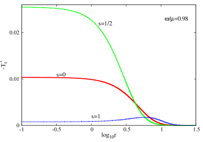
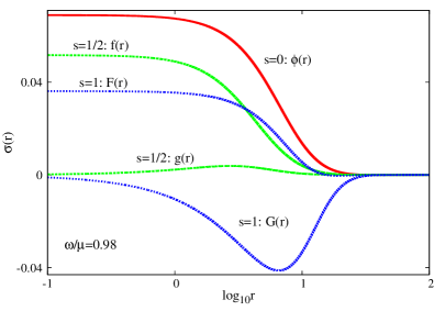
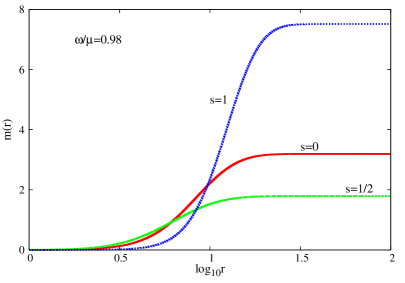
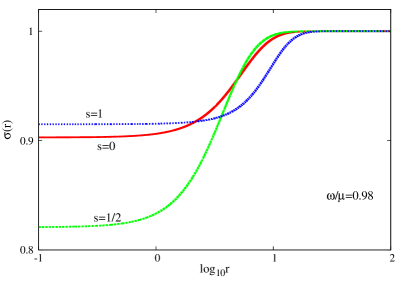
Figure 1: Top left panel: the energy density is shown for a (typical) solution of each spin-$s$ model in $D=5$ dimensions, all with the same frequency to particle mass ratio, $w/\mu=0.98$. Top right panel: the matter functions profiles for the same solutions. Bottom panels: the metric functions are shown for the same solutions.

Finally, the virial identity satisfied by the solutions reads

$$\int_{0}^{\infty}dr~{}r^{D-2}\sigma\left((D-2)^{2}\frac{fg}{r}+\frac{(2(D-1)+(D+1)(N-1))}{2\sqrt{N}}(gf^{\prime}-fg^{\prime})\right)=$$ (38)

$$\int_{0}^{\infty}dr~{}r^{D-2}\sigma\left(\frac{w(f^{2}+g^{2})}{2N\sqrt{N}}(2(D-1)+(3D-5)(N-1))+(D-1)\mu(f^{2}-g^{2})\right).$$

3 The results

We are interested in particle-like solutions of the eqs. (11), (12), (17), (18) and (35), (37), with a topologically trivial, smooth geometry and a regular matter distribution. Thus, as $r\to 0$, one imposes $N(r)\to 1$ (with $m(r)\sim O(r^{D-1})$), while $\sigma(r)\to\sigma_{0}>0$. The requirement of finite mass and asymptotic flatness imposes $m(r)\to m_{0}$ ($i.e.$ $N(r)\to 1$) and $\sigma(r)\to 1$ as $r\to\infty$. Also, all matter functions vanish ar infinity, while their behaviour near the origin is more complicated, with $f(r)$ and $G(r)$ vanishing there, while $\phi(r)$, $g(r)$ and $F(r)$ satisfy Neumann boundary conditions. For any $s$, an approximate form of the solutions can be systematically constructed in both regions, near the origin and for large values of $r$. For example, the near-origin expansion contains two free parameters, one of them being $\sigma(0)$, and the other one being $\phi(0)$, $g(0)$ or $F(0)$, while the matter fields decay exponentially in the far field.

The solutions that smoothly interpolate between these asymptotics are constructed numerically. The results reported in this work are found in units with $\mu=1$, $4\pi G=1$ (thus we use a scaled radial coordinate $r\to r/\mu$ (together with $m\to m/\mu^{D-3}$, $w\to w\mu$ and, for $s=1/2$, $f\to f\sqrt{\mu}$, $g\to g\sqrt{\mu}$) while the factor of $4\pi G$ is absorbed in the expression of the matter functions). The equations are solved by using a standard Runge-Kutta ODE solver and implementing a shooting method in terms of the near-origin essential parameters, integrating towards $r\to\infty$.

For a given spin-$s$ model, the only input parameters are the number $D$ of spacetime dimensions and the value $w$ of the frequency. Then a (presumably infinite) set of solutions is found for some range of $w$, as indexed by the number of nodes of the matter functions. Note that, however, only fundamental solutions are reported in this work.

We have constructed in a systematic way scalar, Proca and Dirac stars in $D=4,5$ and $6$ dimensions; partial (less accurate) results were also found for $D=7$, $8$. The profile of typical $D=5$ configurations with the same ratio $w/\mu$ are shown in Fig. 1, together with the corresponding energy-density distribution. This plot appears to be generic, a (qualitatively) similar picture being found for other values of $w$ (or even for $D\neq 5$).

Figure 2: The generic $M(w)$-diagram (with $M$ the ADM mass and $w$ the field frequency) is shown for the $s=0,1/2,1$ families of solutions in $D\geq 4$ dimensions.

Remarkably, the $s=0,1/2,1$ solutions exhibit a certain degree of universality, the pattern depending on the number of the spacetime dimensions. Their basic (qualitative) features are displayed in Fig. 2 in a frequency-mass diagram, which is the main result of this work, while quantitative results are shown in Fig. 3.

The study of these plots indicates the existence of a number of basic properties which hold for both bosonic and fermionic solutions and can be summarized as follows.

• For any $D$, a (continuous) family of $s=0,1/2,1$ solutions exists for a limited range of frequencies only, $w_{min}<w<\mu$, the minimal value of the ratio $w/\mu$ decreasing with the spacetime dimension. After reaching the minimal frequency, the $M(w)$-curve backbends into a second branch; moreover, further branches and backbendings are found. We conjecture that, for any $D$, the $M(w)$-curve becomes a spiral, which approaches at its center a critical solution, a result rigorously established so far only for the $D=4,~{}s=0$ case [16], [17].

• The behaviour of the solutions as $w\to\mu$ depends on the number of spacetime dimensions. For $D=4$, the matter field(s) becomes very diluted and the solutions trivialize in that limit, with $M\to 0$, the maximal mass value being attained at some intermediate frequency.

  The picture for $D=5$ is different and a mass gap is found between the $\mathcal{U}=0$ vacuum Minkowski ground state and the set of solutions with $\mathcal{U}\neq 0$. Moreover, the limiting configurations with a frequency $w$ arbitrarily close to $\mu$ exhibit a different pattern as compared to the four dimensional case. That is, although the matter fields spread and tend to zero, while the geometry becomes arbitrarily close to that of flat spacetime, the mass remains finite and nonzero (being also the maximal allowed value).

  The existence of a mass gap is a property found also for $D\geq 6$ solutions. Also, again the solutions do not trivialize as $w\to\mu$. However, in this case their mass appears to diverge in that limit.

• A similar picture is found when considering instead a $Q(w)$ diagram. In particular, one finds that $M>\mu Q$ for all $D>4$ solutions, with (at the level of numerical accuracy) $M\to\mu Q$ as $w\to\mu$. The picture for $D=4$ is more complicated, with $M<\mu Q$ for some range of frequencies ranging between $\mu$ and some critical value [3], [4].

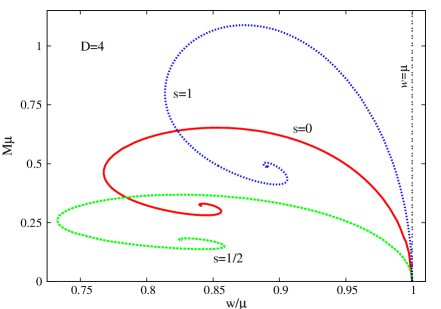
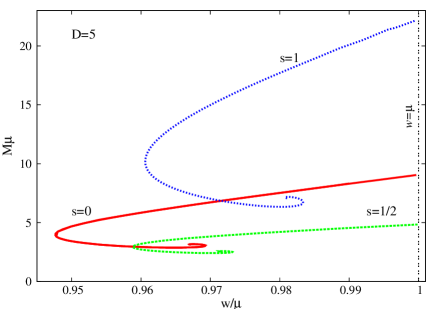
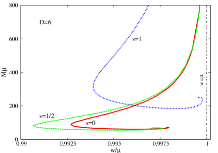
Figure 3: The ADM mass $M$ $vs.$ field frequency $w$ is shown for scalar ($s=0$), Proca ($s=1$ and Dirac $(s=1/2)$ stars in $D=4,5,6$ dimensions.

Figure 4: The ADM mass is shown vs. field mass $\mu$ for Dirac stars in $D=4,~{}5$ and $6$ dimensions. The single particle condition, $Q=1$ for a fermionic field, is imposed here. Note that the $D=6$ curve continues to large values, presumably diverging. The inset focuses on the $D=5$ case.

3.1 Fermions: the single particle condition

In the discussion above, no distinction has been made between the bosonic and fermionic solutions. However, although we have treated the Dirac equation classically, the fermionic nature of a spin $s=1/2$ field would manifest at the level of the occupation number. Thus, for each field $\Psi^{[A]}$, at most a single particle should exist, in accordance to Pauli’s exclusion principle.

The single particle condition, $Q=1$ is imposed by using the following scaling symmetry of the Einstein-Dirac system :

$$r\to\lambda\bar{r},~{}w\to\frac{\bar{w}}{\lambda},~{}\mu\to\frac{\bar{\mu}}{\lambda},~{}m\to\lambda^{D-3}\bar{m},~{}f\to\frac{\bar{f}}{\sqrt{\lambda}},~{}g\to\frac{\bar{g}}{\sqrt{\lambda}},~{}{\rm while}~{}M\to\lambda^{D-3}\bar{M},~{}Q\to\lambda^{D-2}\bar{Q},$$

(with $\lambda>0$ arbitrary and $\sigma$ invariant). One can easily verify that this transformation does not affect the equations of motion; however, it $changes$ the model, since it leads to a different field mass $\mu$. Then, for an initial solution with a given $Q$, the condition $\bar{Q}=1$ is imposed by taking $\lambda=Q^{\frac{1}{D-2}}$, which accordingly changes the corresponding values for the ADM mass and the field’s frequency and mass.

The resulting $M(\mu)$-diagram is shown in Fig. 4 for Einstein-Dirac solutions in $D=4,~{}5$ and 6 dimensions (note that there we drop the overline for both $M$ and $\mu$). Again, one notices a different behaviour in each spacetime dimension. In four dimensions, the ($n_{f}=2$ particle) Einstein-Dirac solutions exist for a family of models with both $\mu$ and $M$ ranging from zero to a maximal value of order one [7]. The situation is different in $D=5$, in which case the minimal value of $\mu$ and $M$ is nonzero (and $n_{f}=2$ again). This feature is preserved by $D=6$ solutions (with $n_{f}=4$ particles); however, no upper bounds for $\mu$ and $M$ appear to exist in that case.

In the inset of Fig. 4, we zoom a part of the $D=5$ curve, revealing a structure of peaks. This behaviour is generic for any dimension $D$, and it is related with the inspiral behaviour commented in the previous section. As a result, one can see that for fixed values the dimension $D$ and the scaled field mass $\mu$ ($i.e.$ for fixed models), it is possible to have situations with a single solution (only one value of $M$), a discrete set of solutions (with different values of $M$), or no solution.

4 Further remarks

The main purpose of this work was to provide a preliminary investigation of a special type of solitonic solutions of gravitating matter systems in a number $D\geq 4$ of spacetime dimensions. The (massive) matter fields correspond to bosons (spin 0, 1) or Dirac fermions (spin $1/2$), respectively, and possess an harmonic time dependence. The simplest solutions of this type are the well-known $D=4$, $s=0$ boson stars [1], [2].

Our results show that, for any $D$, the existence of these particle-like solutions, does not distinguish between the fermionic/bosonic nature of the field, with the existence of a general pattern fixed by the number of spacetime dimensions. Moreover, while the cases $D=4$ and $D=5$ are special, the $D>5$ solutions appear to share the same (qualitative) picture. Perhaps the most curious feature revealed by this study is the existence, for $D>4$, of a mass gap, the set of spin-$s$ configurations being not continuously connected to Minkowski spacetime vacuum.

Among the numerous avenues that one may pursue following the study here we mention a few. First, it would be interesting to clarify the stability of $D>4$ solutions, an issue which has been extensively studied for $D=4$ (see $e.g.$ [3], [4] for $s=0$, [5], [18] for $s=1$, and [6] for the $s=1/2$ case). Since, as noticed above, the higher dimensional configurations have $M>\mu Q$, they possess an excess energy and thus we expect them to be unstable against fission (the case $s=1/2$ being more subtle, due to the single particle condition). A better understanding of the limiting behaviour of the solutions as $w\to\mu$ and towards the center of the $M(w)$-spiral is another important open question. In the scalar field case (with $D=4$), an explanation of this behaviour is provided in [16], [17] (see also the explanation in Ref. [8] for the beaviour of the $D=5$ bosons stars ($s=0$) as $w\to\mu$ ).

Furthermore, one may inquire if, similar to other field theory models [23], these spin-$s$ solitons possess generalizations with a horizon at their center. In four dimensions, no such (spherically symmetric) solutions exist, as shown in [19] for spin 0, in [20] for spin 1 and in [21], [22] for a Dirac field. We expect a similar result to hold also in the higher dimensional case.

Finally, it would be interesting to investigate the solutions in this work within the framework of the large-$D$ limit of General Relativity [24].

References

- [1] D. J. Kaup, Phys. Rev. 172 (1968) 1331.
- [2] R. Ruffini and S. Bonazzola, Phys. Rev. 187 (1969) 1767.
- [3] F. E. Schunck and E. W. Mielke, Class. Quant. Grav. 20 (2003) R301 [arXiv:0801.0307 [astro-ph]].
- [4] S. L. Liebling and C. Palenzuela, Living Rev. Rel. 15 (2012) 6 [arXiv:1202.5809 [gr-qc]].
- [5] R. Brito, V. Cardoso, C. A. R. Herdeiro and E. Radu, Phys. Lett. B 752 (2016) 291 [arXiv:1508.05395 [gr-qc]].
- [6] F. Finster, J. Smoller and S. T. Yau, Phys. Rev. D 59 (1999) 104020 [gr-qc/9801079].
- [7] C. A. R. Herdeiro, A. M. Pombo and E. Radu, Phys. Lett. B 773 (2017) 654 [arXiv:1708.05674 [gr-qc]].
- [8] B. Hartmann, B. Kleihaus, J. Kunz and M. List, Phys. Rev. D 82 (2010) 084022 [arXiv:1008.3137 [gr-qc]].
- [9] M. Heusler and N. Straumann, Class. Quant. Grav. 9 (1992) 2177.
- [10] M. Heusler, Helv. Phys. Acta 69 (1996) 501 [gr-qc/9610019].
-
[11]
S. H. Dong,
Phys. Scripta 67 (2003) 377;
S. H. Dong, J. Phys. A 36 (2003) 4977;
I. I. Cotaescu, Int. J. Mod. Phys. A 19 (2004) 2217 [gr-qc/0306127];
S. K. Chakrabarti, Eur. Phys. J. C 61, 477 (2009) [arXiv:0809.1004 [gr-qc]].
S. H. Dong, “Wave equations in higher dimensions,” Springer, Dordrecht (2011); C. A. Sporea, Mod. Phys. Lett. A 30, 1550145 (2015) [arXiv:1505.00470 [gr-qc]];
J. L. Blázquez-Salcedo and C. Knoll, Phys. Rev. D 97, 044020 (2018) [arXiv:1709.07864 [gr-qc]];
P. A. Gonzalez, Y. Vasquez and R. N. Villalobos, Phys. Rev. D 98, 064030 (2018) [arXiv:1807.11827 [gr-qc]]. -
[12]
V. Frolov, P. Krtous and D. Kubiznak,
Living Rev. Rel. 20, 6 (2017)
[arXiv:1705.05482 [gr-qc]];
B. Carter and R. G. Mclenaghan, Phys. Rev. D 19, 1093 (1979). - [13] J. L. Blázquez-Salcedo and C. Knoll, “Spherically symmetric stress-energy tensor of spinors in static, spherically symmetric spacetimes,” to appear.
-
[14]
T. T. Wu and C. N. Yang,
Nucl. Phys. B 107, 365 (1976);
J. G. Pereira and P. Leal Ferreira, Rev. Bras. Fis. 11, 937 (1981);
R. Camporesi and A. Higuchi, J. Geom. Phys. 20, 1 (1996) [gr-qc/9505009]. -
[15]
J. L. Blázquez-Salcedo and C. Knoll,
Phys. Rev. D 99, 024026 (2019)
[arXiv:1808.00503 [gr-qc]];
J. L. Blázquez-Salcedo and C. Knoll, arXiv:1811.02014 [gr-qc]. - [16] R. Friedberg, T. D. Lee and A. Sirlin, Phys. Rev. D 13 (1976) 2739.
- [17] R. Friedberg, T. D. Lee and Y. Pang, Phys. Rev. D 35, 3640 (1987).
- [18] N. Sanchis-Gual, C. Herdeiro, E. Radu, J. C. Degollado and J. A. Font, Phys. Rev. D 95 (2017) no.10, 104028 [arXiv:1702.04532 [gr-qc]].
- [19] I. Pena and D. Sudarsky, Class. Quant. Grav. 14 (1997) 3131.
- [20] C. Herdeiro, E. Radu and H. Runarsson, Class. Quant. Grav. 33 (2016) no.15, 154001 [arXiv:1603.02687 [gr-qc]].
- [21] F. Finster, J. Smoller and S. T. Yau, J. Math. Phys. 41 (2000) 2173 [gr-qc/9805050].
- [22] F. Finster, J. Smoller and S. T. Yau, Commun. Math. Phys. 205 (1999) 249 [gr-qc/9810048].
-
[23]
M. S. Volkov and D. V. Gal’tsov,
Phys. Rept. 319 (1999) 1
[hep-th/9810070];
C. A. R. Herdeiro and E. Radu, Int. J. Mod. Phys. D 24 (2015) no.09, 1542014 [arXiv:1504.08209 [gr-qc]];
M. S. Volkov, “Hairy black holes in the XX-th and XXI-st centuries,” arXiv:1601.08230 [gr-qc]. - [24] R. Emparan, R. Suzuki and K. Tanabe, JHEP 1306 (2013) 009 [arXiv:1302.6382 [hep-th]].