Energy Efficient Beamforming Design for MISO Non-Orthogonal Multiple Access Systems

Abstract

When considering the future generation wireless networks, non-orthogonal multiple access (NOMA) represents a viable multiple access technique for improving the spectral efficiency. The basic performance of NOMA is often enhanced using downlink beamforming and power allocation techniques. Although downlink beamforming has been previously studied with different performance criteria, such as sum-rate and max-min rate, it has not been studied in the multiuser, multiple-input single-output (MISO) case, particularly with the energy efficiency criteria. In this paper, we investigate the design of an energy efficient beamforming technique for downlink transmission in the context of a multiuser MISO-NOMA system. In particular, this beamforming design is formulated as a global energy efficiency (GEE) maximization problem with minimum user rate requirements and transmit power constraints. By using the sequential convex approximation (SCA) technique and the Dinkelbach’s algorithm to handle the non-convex nature of the GEE-Max problem, we propose two novel algorithms for solving the downlink beamforming problem for the MISO-NOMA system. Our evaluation of the proposed algorithms shows that they offer similar optimal designs and are effective in offering substantial energy efficiencies compared to the designs based on conventional methods.

I Introduction

Non-orthogonal multiple access (NOMA) is considered to be a viable and a promising multiple access technique to improve the spectral efficiency (SE) in future wireless networks [1, 2]. More specifically, it is hailed as an avenue to offer an array of benefits including high spectral efficiency, better quality-of-service (QoS), lower latency and massive connectivity [3, 4, 5]. In contrast to the conventional orthogonal multiple access (OMA) technique, NOMA simultaneously sends signals to multiple users using the power-domain multiplexing, while sharing the same time-frequency resources [6]. When performing the power-domain multiplexing [7], multiple signals intended for different users are multiplexed based on superposition coding [5] with different power levels prior to the transmission. At the receiving end, the successive interference cancellation (SIC) technique is employed to decode the incoming signals [8]. Furthermore, the massive connectivity offered by NOMA is perfect for handling the requirements of applications stemming from the area of Internet-of-Things (IoT), where the transmission of very large number of small messages is rather prevalent [9]. In particular, NOMA can also be incorporated into a number of future key distributive technologies, such as massive multi-input multi-output (MIMO) systems and millimeter-wave (mmWave) technologies [10] [11]. The key drive in such applications is to further increase the throughput, particularly in the fifth generation (5G) and beyond wireless networks  [12, 13, 14].

With the progressive adoption of 5G and beyond wireless networks, one of the main goals is to achieve a higher spectral efficiency compared to the ones available in contemporary wireless communications systems. Higher spectral efficiency will enable applications that demand different high data rates and will provide massive connectivity for IoT [15]. With limited available wireless resources, including radio spectrum and transmit power, meeting higher data requirements will only be possible through novel techniques and efficient resource utilizations [16]. Furthermore, the transmit power required to meet the corresponding throughput requirements with the conventional approaches will be significantly high. This increased power consumption will subsequently induce further issues such as extra CO₂ emission and associated climate changes [17]. Recently, energy efficient techniques are considered as one of the key avenues for addressing these issues in the development of future wireless systems [16]. The energy efficient designs based on global energy efficiency (GEE) performance metric have become one of the key requirements in the development of future wireless systems. These designs take the energy efficiency (EE) performance metric into account rather than the achievable rate or transmission power metrics. The GEE performance metric is defined as the ratio between the achievable sum-rate and total power consumption [18, 17]. Furthermore, the GEE design can be viewed as a multi-objective design problem, which aims to simultaneously optimize two conflicting performance metrics, namely, the sum rate and the required power to achieve this sum rate [18]. Furthermore, this performance metric efficiently utilizes the available transmit power while striking a good balance between the achievable sum rate and power consumption. Finally, unlike the conventional sum rate maximization and power minimization designs, the GEE design incorporates the power losses at the base station as part of the design process [17]. The EE performance metric plays a crucial role in the overall performance of a NOMA system due to the fact that it exploits power-domain multiplexing to simultaneously transmit signals to multiple users [4]. Achieving the massive connectivity offered by NOMA requires a huge amount of transmit power which would only be possible by considering energy efficient designs [5]. Therefore, the EE performance metric attracts a great deal of attention from the community, which thrives to develop various novel yet practical techniques including NOMA for future wireless networks.

In the context of NOMA, the core component, the power domain multiplexing, directly dictates the power allocation at the transmitter-level, and thus indirectly controls the overall energy consumption. Hence, the power domain multiplexing, when combined with downlink beamforming, will decide the overall energy performance of a NOMA system. Therefore, considering all the parameters that affect the resulting EE is very crucial for improving the EE of the entire system, particularly at the design level. A number of approaches have been proposed in the literature for this purpose. In [19], a beamforming design to maximize the spectral efficiency is proposed for multiple-input single-output (MISO)-NOMA systems using a variant of the minorization-maximization algorithm [20]. In [21], a power minimization problem is considered in conjunction with the QoS aspect, and an approach based on the second order cone (SOC) programming is proposed. An energy efficient-based power allocation scheme is developed in [22] for a single-input single-output (SISO) NOMA system by utilizing the Karush-Kuhn-Tucker (KKT) conditions [23]. These approaches are complemented by [24], where both the EE and the computational complexity arising out of the SIC operations are addressed. They have proposed a clustering method for maximizing the EE for SISO-NOMA systems, with the approach of assigning the same channel for multiple users. In [25], a max-min fairness based energy efficient design is studied in the context of downlink transmission for SISO-NOMA systems. On the other hand, the authors in [26] consider the EE maximization problem for MIMO-NOMA systems, with multiple users are grouped in a cluster. Whereas, multiple resource allocations strategies and clustering algorithms have been introduced in [27] [28]. Furthermore, the authors in [29] investigated an energy efficiency design for a downlink NOMA single-cell network assuming imperfect channel state information.

To-date, to the best of our knowledge, no study has been conducted on downlink beamforming design for multiuser MISO-NOMA systems, particularly with the focus of maximizing the EE. In this paper, we address this issue, by proposing an energy-efficient downlink beamforming design. We formulate the overall problem as a global energy efficiency maximization (GEE-Max) problem that incorporates the minimum rate requirements and transmit power constraints as part of the formulation. However, as will be seen, due to the non-convex nature of the constraints and because of the overall fractional objective function, the overall GEE-Max formulation is a non-convex optimization problem. With the appropriate and necessary initial evaluations, and through suitable approximations, we overcome the non-convexity issues for solving the GEE-Max problem. We make the following key contributions:

1. Meta-approach for detecting the feasibility of solving GEE-Max: Although the overarching problem can be formulated as a GEE-Max problem, the formulation does not guarantee the solvability of the GEE-Max problem. In fact, it might turn out to be an infeasible problem. We propose an approach to detect this infeasibility at the early stages of problem formulation, and propose an alternative approach;

2. Algorithms for solving the GEE-Max problem: As discussed above, the non-convexity of the GEE-Max problem stems from two aspects: the non-convex nature of the constraints and the fractional nature of the overall objective function. We present two novel iterative algorithms for handling these issues. The first algorithm uses the sequential convex approximation (SCA) technique to approximate the non-convex constraints while the second algorithm utilizes the Dinkelbach’s technique for handling the non-convex nature of the fractional objective function; and

3. Optimality validation: We validate the optimality of the proposed SCA-based GEE-Max algorithm by comparing the optimal solution of an equivalent power minimization problem. In particular, both the algorithm and power minimization problem should lead to identical solutions. However, the power minimization problem is a convex problem, and therefore, the solution is optimal in terms of required transmit power to achieve the corresponding minimum rate at each user. This confirms the optimality of the results obtained through the SCA-based algorithm.

The remainder of the paper is organized as follows. In Section II we present a system model and formulate the problem with necessary feasibility conditions. This is then followed by Section III, where we propose two iterative algorithms, a key part of our contributions. Detailed evaluations and simulation results are presented in Section IV, demonstrating the effectiveness of the proposed algorithms through comparing their performance with different beamforming techniques available in the literature. We then finally conclude the paper in Section V.

In the rest of the paper, we adopt the following notations: We use the lower-case boldface letters for vectors and upper-case boldface letters for matrices; $(\cdot)^{H}$ denotes complex conjugate transpose; $\Re(\cdot)$ and $\Im(\cdot)$ stand for real and imaginary parts of a complex number, respectively; $\mathbb{C}^{N}$ and $\mathbb{R}^{N}$ denote the $N$-dimensional complex and real spaces, respectively; and E($\cdot$), $||\cdot||_{2}$ and $|\cdot|$ represent the expectation, the Euclidean norm of a vector, and absolute value of a complex number, respectively. Tr$(\cdot)$ stands for the trace of a matrix.

II System Model and Problem Formulation

II-A System Model

We consider a downlink transmission of a MISO-NOMA system with $K$ users as shown in Figure 1, where a single base station simultaneously transmits information to all users. We assume that the base station here is equipped with $N$ antennas (i.e., $N>1$) while there is a single antenna at the user’s end. The signal transmitted from the base station can be expressed as:

$$\mathbf{x}=\sum_{k=1}^{K}\mathbf{w}_{k}s_{k},$$ (1)

where $s_{k}$ and $\mathbf{w}_{k}\in\mathbb{C}^{N\times 1}$ denote the signal intended for the $k^{th}$ user and the corresponding beamforming vector, respectively. Note that a digital beamforming is adopted in this work. The power of the transmitted symbol is assumed to be one, i.e., E($|s_{k}|^{2})=1$.

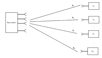
Figure 1: A multiuser, MISO-NOMA system with a multi-antenna base station, and $K$-single antenna users.

The received signal at the $i^{th}$ user can be expressed as:

$$y_{i}=\mathbf{h}_{i}^{H}\mathbf{w}_{i}s_{i}+\sum_{j=1,j\neq i}^{K}\mathbf{h}_{i}^{H}\mathbf{w}_{j}s_{j}+n_{i},$$ (2)

where $\mathbf{h}_{i}\in\mathbb{C}^{N\times 1}$ represents the channel coefficients between the base station and the $i^{th}$ user, and $n_{i}$ represents the zero-mean circularly symmetric complex additive white Gaussian noise with variance $\sigma^{2}$. Furthermore, we define $\mathbf{h}_{i}$ such that $\mathbf{h}_{i}~{}=~{}\sqrt{d_{i}^{-\kappa}}\mathbf{g}_{i}$, where $\kappa,d_{i}$ and $\mathbf{g}_{i}$ denote the path loss exponent, the distance between the $i^{th}$ user and the base station, and small scale fading, respectively. In addition, it is assumed that the base station has the perfect channel state information (CSI) of each user. In NOMA, user ordering plays a crucial role in implementing the SIC at the users’ ends, and in fact, determines the overall performance of the system [6]. However, determining optimal user ordering is an NP-hard problem, which can only be solved through exhaustive search, branch and bound methods or heuristic approaches [4, 30]. In this paper, for the reasons of simplicity, the users are ordered based on their respective channel strengths. Thus, the first user will have the strongest channel strength, while the channel strength of the $K^{th}$ user will be the weakest. As such, the channels can equivalently be ordered as follows:

$${||\mathbf{h}_{K}||_{2}^{2}}\leq{||\mathbf{h}_{K-1}||_{2}^{2}}\leq\cdots\leq{||\mathbf{h}_{1}||_{2}^{2}}.$$ (3)

By employing SIC, the $i^{th}$ user ($U_{i}$) should be able to successively decode and subtract the signals intended for the weaker users $U_{K},\cdots,U_{i-1}$ from the received signal [31]. The received signal after eliminating the last $K-i$ user signals can expressed as:

$$\overset{\sim}{y_{i}}=\mathbf{h}_{i}^{H}\mathbf{w}_{i}s_{i}+\sum_{j=1}^{i-1}\mathbf{h}_{i}^{H}\mathbf{w}_{j}s_{j}+n_{i},$$ (4)

where the first term in (4) represents the intended signal for the $i^{th}$ user, while the second term denotes the interference caused by the first $i-1$ signals intended for users $\{U_{1},\cdots,U_{i-1}\}$. Note that $U_{i}$ perfectly decodes the messages intended to the weaker users without any errors. The achievable signal to interference and noise ratio (SINR) for the $k^{th}$ user to decode the signal that is intended to the $i^{th}$ user is:

$$SINR_{k}^{i}=\frac{|\mathbf{h}_{k}^{H}\mathbf{w}_{i}|^{2}}{\sum_{j=1}^{i-1}|\mathbf{h}_{k}^{H}\mathbf{w}_{j}|^{2}+\sigma_{k}^{2}},i\in\mathcal{K},\forall k\leq i.$$ (5)

It is inherently clear that (5) holds true only after performing SIC on the preceding $k-i$ signals. Furthermore, $\mathcal{K}\overset{\bigtriangleup}{=}\{1,2,\cdots,K\}.$ To successfully decode the $i^{th}$ signal at the $k$ strong users (i.e., $k<i$), the achievable SINR of decoding the $i^{th}$ signal at the $k^{th}$ user, $\gamma_{k}^{i}$, should be greater than a predefined threshold $\gamma_{th}$. This condition can be mathematically defined as in [19] [32]. Thus,

$${\gamma}_{i}=\min({\gamma^{i}_{1},\gamma^{i}_{2},\cdots,\gamma^{i}_{k},\cdots,\gamma^{i}_{i}})\geq\gamma_{th},$$ (6)

therefore, the achievable rate $R_{i}$ for the user $U_{i}$ can be defined as follows:

$$R_{i}=B_{w}\log_{2}(1+{\gamma}_{i}),\forall i\in\mathcal{K},$$ (7)

where $B_{w}$ is the available bandwidth. For notational simplicity, we assume that $B_{w}=1$ in the rest of this paper. Furthermore, the user with the weakest channel strength may not be able to achieve a reasonable rate, owing to the fact that significant amount of transmit power must have already been allocated. To circumvent this problem, the following condition should also be satisfied to maintain a rate fairness between users with different channel strengths [33]:

$$|\mathbf{h}_{i}^{H}\mathbf{w}_{K}|^{2}\geq|\mathbf{h}_{i}^{H}\mathbf{w}_{K-1}|^{2}\geq\cdots\geq|\mathbf{h}_{i}^{H}\mathbf{w}_{1}|^{2},$$ (8)

where $i\in\mathcal{K}$. The constraint expressed in (8) will be referred to as the SIC constraint in the rest of this paper.

II-B Problem Formulation

For the MISO-NOMA system defined above, we consider an energy efficient maximization problem. In particular, this energy efficient optimization problem is formulated to maximize the GEE of the system satisfying the available total power at the base station, and the minimum rate requirement of each user. The total power consumption at the base station accounts for both the transmit power allocated for data transmission and the power losses. As for the required transmit power $P_{tr}$, it should satisfy the available power budget, $P_{ava}$, at the base station, which can be mathematically formulated as the following constraint:

$$P_{tr}=\sum_{i=1}^{K}{||\mathbf{w}_{i}||_{2}^{2}}\leq P_{ava}.$$ (9)

As for the power losses at the base station, denoted by $P_{loss}$, they should account both the dynamic and static power losses $p_{dyn}$ and $p_{sta}$, respectively. The former primarily depends on the number of transmit antennas $N$, whereas the latter is intended to account for the power required to maintain the system, such as through cooling and conditioning. The total power losses can be defined as in [18]:

$$P_{loss}=p_{sta}+Np_{dyn}.$$ (10)

Hence, the total power consumption at the base station is:

$$P_{total}=\frac{1}{\epsilon_{0}}P_{tr}+P_{loss},$$ (11)

where $0<\epsilon_{0}\leq 1$ is the efficiency of the power amplifier.

The GEE of the system is defined as the ratio between the total achievable sum rate and the total power consumption,

$$GEE=\frac{\sum_{i=1}^{K}R_{i}}{P_{total}}.$$ (12)

With these definitions in place, the beamforming design to maximize the GEE in a MISO-NOMA system with $K$ users can be formulated into the following optimization framework:

$${{OP}_{1}\text{:}~{}} \underset{\{\mathbf{w}_{i}\}_{i=1}^{K}}{\text{maximize }} \!\!\!\!\!\!\frac{\sum_{i=1}^{K}\log{(1+\gamma_{i})}}{\frac{1}{\epsilon_{0}}\sum_{i=1}^{K}||\mathbf{w}_{i}||^{2}_{2}+P_{loss}}$$ (13a)

subject to $$\!\!\!\!\!\!R_{i}\geq R^{\text{min}}_{i},\,\forall i\in\mathcal{K},$$ (13b)

$$\!\!\!\!\!\!\sum_{i=1}^{K}||\mathbf{w}_{i}||^{2}_{2}\leq P_{ava},$$ (13c)

$$\!\!\!\!\!\!(\ref{eqn:channels}),$$ (13d)

where $R_{i}^{min}$ is the minimum rate requirement for the user $U_{i}$, and (13d) ensures the successful implementation of the SIC for all users while maintaining the rate fairness between them.

II-C Feasibility Conditions

The optimization problem $OP_{1}$ defined in (13) is worth solving only when it is feasible to solve for a given set of constraints. For instance, the $OP_{1}$ problem may not be solvable because of insufficient available power budget at the base station, or higher user data rate requirements. As such, it is first worth verifying the feasibility conditions prior to attempting to solve the GEE-Max problem. We outline an approach for verifying the feasibility conditions using the power minimization (P-Min) problem with minimum data rate requirements and user rate fairness constraints:

$${OP_{2}}\text{:}~{}P^{*}\text{=}~{} \underset{\{\mathbf{w}_{i}\}_{i=1}^{K}}{\text{minimize }} \!\!\!\!\!\!\sum_{i=1}^{K}||\mathbf{w}_{i}||^{2}_{2}$$ (14a)

subject to $$\!\!\!\!\!\!R_{i}\geq R^{\text{min}}_{i},\forall i\in\mathcal{K},$$ (14b)

$$\!\!\!\!\!\!(\ref{eqn:channels}),$$ (14c)

where $P^{*}$ denotes the minimum power required to achieve the minimum rate and satisfy the SIC constraints. The above optimization problem, $OP_{2}$, has been solved in [21] by handling the non-convex constraints through a set of convex approximation techniques, which are detailed in the next section. If $P^{*}>P_{ava}$, then the optimization problem in $OP_{1}$ can be classified as an infeasible problem. To overcome this infeasibility issue, we consider the following sum-rate maximization (SRM) problem, where the achievable sum-rate is maximized with transmit power constraint and SIC constraints. This SRM problem can be formulated as in [19]:

$${OP_{3}}\text{:}~{} \underset{\{\mathbf{w}_{i}\}_{i=1}^{K}}{\text{maximize }} \!\!\!\!\!\!{\sum_{i=1}^{K}\log{(1+\gamma_{i})}}$$ (15a)

subject to $$\!\!\!\!\!\!\sum_{i=1}^{K}||\mathbf{w}_{i}||^{2}_{2}\leq P_{ava},$$ (15b)

$$\!\!\!\!\!\!(\ref{eqn:channels}).$$ (15c)

The optimization problem $OP_{3}$ is solved as in [19] using the SCA technique. It is worth to explore an efficient method to solve the original GEE-Max problem in $OP_{1}$, provided that the problem is feasible. In the following section, we develop two iterative algorithms to determine a solution with the assumption that the minimum data requirements and the SIC constraints can be met within the available power budget.

III Algorithms for Solving the GEE-Max Problem

The GEE-Max problem defined in (13) is a non-convex problem due to non-convex objective function and constraints. Hence, it is challenging to obtain an optimal solution. In this section, we develop two iterative algorithms to determine the beamforming vectors to maximize the GEE of the system while satisfying the respective constraints. These algorithms are proposed by approximating the non-convex objective function and constraints to convex ones based on the SCA and Dinkelbach’s algorithms. The details of the algorithms are provided in the following two subsections.

III-A Approach based on the Sequential Convex Approximation

Sequential convex approximation or sequential convex programming [34] is one of the well-known techniques that has been widely adopted to approximate and transform non-convex problems to convex problems. A number of studies demonstrate the viability of this approach in real-world applications [19, 17]. The basic idea of SCA is to establish a convex trust region around the original non-convex spatial points, so that the overall objective function is sequentially optimized for every spatial point. As such, it is a heuristic-driven approach, where the optimality of the ultimate solution may vary depending on the initialization. In our case, by introducing a slack variable $\alpha$, the original problem specified by $OP_{1}$ can be reformulated in the following epigraph form:

$$\underset{\{\mathbf{w}_{i}\}_{i=1}^{K}}{\text{maximize }} \!\!\!\!\!\!\alpha$$ (16a)

subject to $$\!\!\!\!\!\!\frac{\sum_{i=1}^{K}\log{(1+\gamma)}}{\frac{1}{\epsilon_{0}}\sum_{i=1}^{K}||\mathbf{w}_{i}||^{2}_{2}+P_{loss}}\geq\sqrt{\alpha},$$ (16b)

$$\!\!\!\!\!\!R_{i}\geq R^{\text{min}}_{i},\,\forall i\in\mathcal{K},$$ (16c)

$$\!\!\!\!\!\!\sum_{i=1}^{K}||\mathbf{w}_{i}||^{2}_{2}\leq P_{ava},$$ (16d)

$$\!\!\!\!\!\!(\ref{eqn:channels}),$$ (16e)

where the objective function in the original problem (13) is replaced by $\sqrt{\alpha}$ (or equivalently ${\alpha}$). Without loss of generality, the non-convex constraint with the slack variable $\alpha$ in (16b) can equivalently be decomposed into the following two constraints:

$$\sum_{i=1}^{K}\log{(1+\gamma_{i})}\geq\sqrt{\alpha\beta},$$ (17a)

$$\frac{1}{\epsilon_{0}}\sum_{i=1}^{K}{||\mathbf{w}_{i}||_{2}^{2}}+P_{loss}\leq\sqrt{\beta}.$$ (17b)

By incorporating the definition of SINR_i (i.e., $\gamma_{i}$) in (6), the constraint in (17a) can be represented as follows:

$$\sum_{i=1}^{K}\log{(1+\min({\gamma^{i}_{1},\gamma^{i}_{2},\cdots,\gamma^{i}_{k},\cdots,\gamma^{i}_{i}}))}\geq\sqrt{\alpha\beta}.$$ (18)

To handle the non-convexity of (18), we firstly introduce a set of new slack variables such that:

$$\log{(1+\min({\gamma^{i}_{1},\gamma^{i}_{2},\cdots,\gamma^{i}_{k},\cdots,\gamma^{i}_{i}}))}\geq\delta_{i},\forall i\in\mathcal{K},$$ (19a)

$$(1+{\min({\gamma^{i}_{1},\gamma^{i}_{2},\cdots,\gamma^{i}_{k},\cdots,\gamma^{i}_{i}})})\geq\zeta_{i},\forall i\in\mathcal{K}.$$ (19b)

Based on these new slack variables, the constraint in (19a) can equivalently be represented by the following set of constraints:

$$(\ref{eqn:min})\Leftrightarrow \sum_{i=1}^{K}\delta_{i}\geq\sqrt{\alpha\beta},$$ (20a)

$$(\ref{eqn:min})\Leftrightarrow \zeta_{i}\geq 2^{\delta_{i}},\quad\forall i\in\mathcal{K}.$$ (20b)

However, the constraint in (20a) still remains non-convex. In order to relax this, we exploit the first-order Taylor series, providing approximations around the values of $(\alpha^{(n-1)},\beta_{k,i}^{(n-1)})$. With this,

$$\sum_{i=1}^{K}\delta_{i}\geq\sqrt{\alpha^{(n-1)}\beta^{(n-1)}}+\\ 0.5\sqrt{\frac{\alpha^{(n-1)}}{\beta^{(n-1)}}}(\beta^{(n)}-\beta^{(n-1)})\\ +0.5\sqrt{\frac{\beta^{(n-1)}}{\alpha^{(n-1)}}}(\alpha^{(n)}-\alpha^{(n-1)}).$$ (21)

To handle the constraint expressed in (19b), we introduce another slack variable, $\theta_{k,i}\in\mathbb{R}^{1}_{+}$ ($\forall i\in\mathcal{K},k\leq i$ ), and reformulate the constraint in (19b) into the following set of equivalent constraints, with $\forall i\in\mathcal{K}$ and $k\leq i$,

$$|\mathbf{h}_{k}^{H}\mathbf{w}_{i}|^{2}\geq(\zeta_{i}-1)\theta_{k,i},$$ (22a)

$$\sum_{j=1}^{i-1}|\mathbf{h}_{k}^{H}\mathbf{w}_{j}|^{2}+\sigma_{i}^{2}\leq{\theta_{k,i}}.$$ (22b)

Without any loss of generality, the constraint in (22a), can be re-expressed by introducing an arbitrary rotation to the phase of the beamforming vector $\mathbf{w}_{i}$ such that $\mathbf{h}_{k}^{H}\mathbf{w}_{i}$ becomes real, while the imaginary part $\Im(\mathbf{h}_{k}^{H}\mathbf{w}_{i})$ becomes zero. This change, however, does not alter the original optimization problem nor the solution owing to the fact that this change in the beamformer does not modify the required transmit power or the achieved SINR of any users [35]. Therefore, the constraint covered by (22a) can equivalently be expressed as follows:

$$\Re{(\mathbf{h}_{k}^{H}\mathbf{w}_{i})}\geq\sqrt{({\zeta_{i}-1)}\theta_{k,i}},$$ (23)

where the right side of the above inequality can be approximated using the first-order Taylor series, and the inequality in (23) becomes:

$${\Re(\mathbf{h}_{k}^{H}\mathbf{w}^{(n)}_{i})}\geq\sqrt{{(\zeta_{i}^{(n-1)}-1)}\theta_{k,i}^{(n-1)}}\\ +0.5\sqrt{\frac{({\zeta_{i}^{(n-1)}-1)}}{\theta_{k,i}^{(n-1)}}}(\theta_{k,i}^{(n)}-\theta_{k,i}^{(n-1)})\\ +0.5\sqrt{\frac{\theta_{k,i}^{(n-1)}}{{(\zeta_{i}^{(n-1)}-1)}}}(\zeta_{i}^{(n)}-\zeta_{i}^{(n-1)}).$$ (24)

On the other hand, the non-convex constraint in (22b) can be formulated into a SOC as in [36]:

$$\begin{split}\frac{\theta_{k,i}^{(n)}-\sigma_{i}^{2}+1}{2}&\geq{||{\mathbf{v}_{k}^{(n)}}||}_{2},\end{split}$$ (25)

where

$$\mathbf{v}_{k}^{(n)}=\Bigl{[}\mathbf{h}_{k}^{H}\mathbf{w}^{(n)}_{1}\ldots\mathbf{h}_{k}^{H}\mathbf{w}^{(n)}_{i-1}~{}\phi_{i,k}\Bigr{]}^{T}$$ (26)

and

$$\phi_{i,k}^{n}=\frac{(\theta_{k,i}^{(n)}-\sigma_{i}^{2})-1}{2}.$$ (27)

The non-convexity of the constraint in (17b) can be handled by introducing new slack variable $\beta_{\beta}$ and expressed into multiple, yet equivalent, constraints as follows:

$$\sqrt{\beta}\geq\beta_{\beta},$$ (28a)

$$\beta_{\beta}\geq\frac{1}{\epsilon_{0}}\sum_{i=1}^{K}{||\mathbf{w}_{i}||_{2}^{2}}+P_{loss}.$$ (28b)

This can further be formulated into the following SOC constraints [23]:

$$\frac{\beta+1}{2} \geq{\Bigl{\|}\Bigl{[}\frac{\beta-1}{2}\quad\beta_{\beta}\Bigr{]}^{T}\Bigr{\|}_{2}},$$ (29a)

$$\frac{(\beta_{\beta}-{P_{loss}})+1}{2} \geq{\Bigl{\|}\Bigl{[}w_{0}~{}\frac{\mathbf{w}_{1}}{\sqrt{\epsilon_{0}}}\ldots\frac{\mathbf{w}_{K}}{\sqrt{\epsilon_{0}}}\Bigr{]}^{T}\Bigr{\|}_{2}},$$ (29b)

where:

$$w_{0}=\frac{(\beta_{\beta}-{P_{loss}})-1}{2}.$$ (30)

Having approximated the original non-convex objective function in (13a) by introducing a number of slack variables, the final form is such that the problem is same as:

$$(\ref{eqn:frac})\Leftrightarrow \text{maximize}\quad\alpha$$

$$(\ref{eqn:frac})\Leftrightarrow \text{subject to}~{}(\ref{eqn:part2}),(\ref{eqn:joodeh}),(\ref{eqn:tata}),$$

$$(\ref{eqn:frac})\Leftrightarrow \quad\quad\quad\quad\quad(\ref{eqn:tata1}),(\ref{eqn:wssdq}),(\ref{eqn:wq1s}).$$

With this, we handle other non-convex constraints in the original GEE-Max problem expressed by $OP_{1}$. Without the loss of generality, the minimum rate constraint in (13b) can be expressed as:

$$\gamma^{i}_{k}\geq\gamma_{i}^{min},\forall i\in\mathcal{K},k\leq i,$$ (32)

where $\gamma_{i}^{min}=2^{R_{i}^{min}}-1$. Furthermore, this SINR constraint can be formulated into an SOC by introducing an arbitrary phase rotation as in (22a) and with $\forall i\in\mathcal{K},k\leq i$

$$\frac{1}{\sqrt{\gamma_{i}^{min}}}\Re(\mathbf{h}_{k}^{H}\mathbf{w}_{i})\geq{\Bigl{\|}\Bigl{[}\mathbf{h}_{k}^{H}\mathbf{w}_{1}\ldots\mathbf{h}_{k}^{H}\mathbf{w}_{i-1}~{}\sigma_{k}\Bigr{]}^{T}\Bigr{\|}_{2}}.$$ (33)

The non-convexity of the constraint in (13d) can be approximated to a convex constraint by applying the first-order Taylor series approximation. However, instead of applying the Taylor series expansion to the original equation, we define a new proxy function $f(\psi_{i,j})$ by stacking the real and imaginary parts of the product $\mathbf{h}_{i}^{H}\mathbf{w}_{j}$ as follows:

$$f(\psi_{i,j}) = {|\mathbf{h}_{i}^{H}\mathbf{w}_{j}|^{2}}$$ (34)

$$= |{|[\Re(\mathbf{h}_{i}^{H}\mathbf{w}_{j})~{}\Im({\mathbf{h}_{i}^{H}\mathbf{w}_{j}})]^{T}||^{2}},$$

where $\psi_{i,j}=[\Re(\mathbf{h}_{i}^{H}\mathbf{w}_{j})~{}\Im({\mathbf{h}_{i}^{H}\mathbf{w}_{j}})]$. We then apply the first-order Taylor series expansion to this proxy function $f(\psi_{i,j})$, and consider two most significant terms:

$$f(\psi_{i,j}^{(n)})\cong f(\psi_{i,j}^{(n-1)})+2(\psi_{i,j}^{(n-1)})^{T}(\psi_{i,j}^{(n)}-\psi_{i,j}^{(n-1)}).$$ (35)

With this approximation in place, each element in the inequality constraint in (13d) can be replaced by the following linear function:

$$\left\lVert\mathbf{h}_{k}^{H}\mathbf{w}_{j}^{(n)}\right\rVert_{2}^{2}\cong\\ \left\lVert\begin{bmatrix}{r}_{k,j}^{(n-1)}\\ {i}_{k,j}^{(n-1)}\end{bmatrix}\right\rVert_{2}^{2}+2\begin{bmatrix}{r}_{k,j}^{(n-1)}\\ {i}_{k,j}^{(n-1)}\end{bmatrix}\begin{bmatrix}{r}_{k,j}^{(n)}-{r}_{k,j}^{(n-1)}\\ {i}_{k,j}^{(n)}-{i}_{k,j}^{(n-1)}\end{bmatrix}^{T},$$ (36)

where

$${r}_{k,j}^{(n)}=\Re{(\mathbf{h}_{k}^{H}\mathbf{w}_{j}^{(n)})},$$ (37)

and

$${i}_{k,j}^{(n)}=\Im{(\mathbf{h}_{k}^{H}\mathbf{w}_{j}^{(n)})}.$$ (38)

By incorporating all of these approximations, the original GEE-Max problem in (13) can be formulated into the following approximated problem:

$$\underset{\Lambda}{\text{maximize }} \alpha$$ (39a)

subject to $$(\ref{eqn:sa7ar}),(\ref{eqn:asad}),(\ref{eqn:tata}),(\ref{eqn:tata1}),(\ref{eqn:const}),$$ (39b)

$$(\ref{eqn:joodeh}),(\ref{eqn:wssdq}),(\ref{eqn:wq1s}),(\ref{eqn:sa77ar}).$$ (39c)

Note that we replaced (36) instead of each term in the inequality in (13d), and $\forall i\in\mathcal{K},k\leq i$, wherever applicable. Furthermore, the expression

$$\Lambda^{(n)}\overset{\bigtriangleup}{=}\{\mathbf{w}_{i}^{(n)},\alpha^{(n)},\beta^{(n)},\beta_{\beta}^{(n)},\theta_{k,i}^{(n)},\zeta_{i}^{(n)},\delta_{i}^{(n)}\}_{i=1}^{K}$$

indicates the $n^{th}$ iteration of the optimization parameters. In particular, the original GEE-Max problem will be iteratively solved using the approximated convex problem in (39). As such, the optimization parameter is initialized with $\Lambda^{(0)}$. In particular, the random selection of $\Lambda^{(0)}$ determines both the feasibility and the convergence of (39). Hence, we initialize $\Lambda^{(0)}$ by evaluating the beamforming vectors first that satisfy the constraints specified by the optimization problem in (14), where the initial slack variables $\alpha^{(0)},\beta^{(0)},\beta_{\beta}^{(0)},\theta_{k,i}^{(0)},\zeta_{i}^{(0)}$ and $\delta_{i}^{(0)}$ are found by substituting these initial beamforming vectors in (17a), (17b), (28a), (22b), (22a), and (19b), respectively. We summarize the algorithm developed to determine the solution of the original GEE-Max problem in Algorithm 1. The algorithm is terminated when the absolute difference between two sequential optimal values is less than a pre-defined threshold $\varepsilon$ (i.e., $|\alpha^{(n)}-\alpha^{(n-1)}|<\varepsilon$).

Algorithm 1 GEE-Max using SCA

Step 1: Initialization of $\Lambda^{(0)}$

Step 2: Repeat

1. Solve the optimization problem in (39).

2. Update $\Lambda^{(n)}$ .

Step 3: Until required accuracy is achieved.

III-B Approach based on the Dinkelbach’s Algorithm

In this subsection, we develop another approach based on the Dinkelbach’s algorithm to solve the GEE-Max problem in $OP_{1}$. In addition to offering an alternative, this approach also helps to compare and validate the performance of the SCA-based algorithm, and minimize the number of required slack variables in the algorithm. Furthermore, although the SCA-based algorithm was useful in transforming the non-convex constraints into convex ones, the fractional nature of the objective function in $OP_{1}$ still remains untouched. We address this issue by introducing an additional non-negative variable, and by representing the objective function by a parametrized, yet equivalent, non-fractional function. The non-negative variable we introduce here, $\chi$, based on [37], is as follows:

$${OP_{5}}\text{:}~{}{\text{maximize }} \Big{(}{\sum_{i=1}^{K}\log{(1+\gamma_{i})}}-$$

$$\chi\big{(}{\frac{1}{\epsilon_{0}}\sum_{i=1}^{K}||\mathbf{w}_{i}||^{2}_{2}+P_{loss}\big{)}}\Big{)}$$ (40a)

subject to $$R_{i}\geq R^{\text{min}}_{i},\,\forall i\in\mathcal{K},k\leq i,$$ (40b)

$$\sum_{i=1}^{K}||\mathbf{w}_{i}||^{2}_{2}\leq P_{ava},$$ (40c)

$$(\ref{eqn:channels}).$$ (40d)

For the reasons of notational simplicity, we denote the numerator and the denominator of the objective function in $OP_{1}$ by $f_{1}$ and $f_{2}$, respectively, such that

$${f_{1}(\{\mathbf{w}_{i}\}_{i=1}^{K})}={\sum_{i=1}^{K}\log{(1+\gamma_{i})}},$$ (41a)

$${f_{2}(\{\mathbf{w}_{i}\}_{i=1}^{K})}={\frac{1}{\epsilon_{0}}\sum_{i=1}^{K}||\mathbf{w}_{i}||^{2}_{2}+P_{loss}}.$$ (41b)

In order to realize the relationship between $OP_{1}$ and $OP_{5}$, we present the following theorem  [37]:

Theorem 1

A necessary and sufficient condition for

$$\chi^{*}=\underset{\{\mathbf{w}_{i}\}_{i=1}^{K}}{\text{maximize}}\frac{f_{1}(\{\mathbf{w}_{i}\}_{i=1}^{K})}{f_{2}(\{\mathbf{w}_{i}\}_{i=1}^{K})}=\frac{f_{1}(\{\mathbf{w}^{*}_{i}\}_{i=1}^{K})}{f_{2}(\{\mathbf{w}^{*}_{i}\}_{i=1}^{K})},$$ (42)

is

$$F({\{\mathbf{w}_{i}}\}_{i=1}^{K},\chi^{*})=\\ \underset{\{\mathbf{w}_{i}\}_{i=1}^{K}}{\text{maximize}}\Big{(}f_{1}(\{\mathbf{w}_{i}\}_{i=1}^{K})-\chi^{*}f_{2}(\{\mathbf{w}_{i}\}_{i=1}^{K})\Big{)}\\ =f_{1}(\{\mathbf{w}_{i}^{*}\}_{i=1}^{K})-\chi^{*}f_{2}(\{\mathbf{w}_{i}^{*}\}_{i=1}^{K})=0,$$ (43)

where $\{\mathbf{w}^{*}_{i}\}_{i=1}^{K}$ are the solution of the original GEE-Max problem.

Proof: Please refer to Appendix A.

Theorem 1 confirms that obtaining the beamforming vectors that maximize the GEE in the original problem $OP_{1}$ is the same as solving the parametrized optimization problem $OP_{5}$. However, the precondition is that the non-negative parameter $\chi$ is a solution of (43), while $F(\chi)$ has a unique solution for any set of $\{\mathbf{w}_{i}\}_{i=1}^{K}$ as in [37]. In this approach, the design variables $\chi$ and $\{\mathbf{w}_{i}\}_{i=1}^{K}$ in $OP_{5}$ are iteratively optimized by exploiting the Dinkelbach’s algorithm. First, the parameter $\chi$ is initialized with zero and the parametrized optimization problem in (40) can be solved using convex approximation techniques [23]. For a given set of beamformers, the design parameter in the $n^{th}$ iteration $\chi$ is updated as follows:

$$\chi^{(n)}=\frac{f_{1}(\{{{\mathbf{w}}}^{(n-1)}_{i}\}_{i=1}^{K})}{f_{2}(\{{{\mathbf{w}}}^{(n-1)}_{i}\}_{i=1}^{K})}.$$ (44)

In particular, the beamforming vectors in the $n^{th}$ iteration ($\{\mathbf{w}^{(n)}_{i}\}_{i=1}^{K}$) can be found by solving the following optimization problem:

$$\underset{\{\mathbf{w}^{(n)}_{i}\}_{i=1}^{K}}{\text{maximize }}\Big{(} {\sum_{i=1}^{K}\log{(1+\gamma_{i})}}-$$

$$\chi^{(n-1)}\big{(}{\frac{1}{\epsilon_{0}}\sum_{i=1}^{K}||\mathbf{w}_{i}^{(n)}||^{2}_{2}+P_{loss}\big{)}}\Big{)}$$ (45a)

subject to $$R_{i}\geq R^{\text{min}}_{i},\forall i\in\mathcal{K},k\leq i,$$ (45b)

$$\sum_{i=1}^{K}||\mathbf{w}_{i}^{(n)}||^{2}_{2}\leq P_{ava},$$ (45c)

$$(\ref{eqn:channels}).$$ (45d)

Due to the non-convex objective function and the non-convex constraints of the optimization problem in (45), we develop an iterative algorithm using the SCA approach. Hence, the objective function is reformulated to a concave form and it is obvious that $\big{(}\frac{1}{\epsilon_{0}}\sum_{i=1}^{K}||$ $\mathbf{w}^{(n)}_{i}||^{2}_{2}+P_{loss}\big{)}$ is convex. Hence, without any loss of generality, multiplying it with $-\chi^{(n)}$ will ensure the concavity of this part. On the other hand, the first part of the objective function (i.e., $\sum_{i=1}^{K}\log{(1+\gamma_{i})})$ requires some relaxations to convert it to a concave form. To this end, we first introduce a new slack variable such that:

$$\sum_{i=1}^{K}\log{(1+\gamma_{i})}\geq\nu,$$ (46)

where the left side of the inequality in (46) can be approximated by incorporating new slack variables ${z}_{i}$ and ${q}_{i}$, such that

$$1+\gamma_{i}\geq z_{i},\forall i\in\mathcal{K},$$ (47a)

$$z_{i}\geq 2^{q_{i}},\forall i\in\mathcal{K}.$$ (47b)

Hence, the non-convex constraint in (46) can be equivalently rewritten as

$$\sum_{i=1}^{K}{q_{i}}\geq\nu.$$ (47c)

Without any loss of generality, we can address the non-convexity of the constraint in (47a) by following the same approach that has been developed to approximate the constraint in (19b) in the previous subsection. In particular, we replace $\zeta_{i}$ and $\theta_{k,i}$ in (22a) and (22b) by $z_{i}$ and $\rho_{k,i}$, respectively. The constraint in (47a) can be equivalently re-written as a set of the following convex constraints:

$${\Re(\mathbf{h}_{k}^{H}\mathbf{w}_{i}^{(n)})}\geq\sqrt{({z_{i}^{(n-1)}-1)}\rho_{k,i}^{(n-1)}}\\ +0.5\sqrt{\frac{({z_{i}^{(n-1)}-1)}}{\rho_{k,i}^{(n-1)}}}(\rho_{k,i}^{(n)}-\rho_{k,i}^{(n-1)})\\ +0.5\sqrt{\frac{\rho_{k,i}^{(n-1)}}{({z_{i}^{(n-1)}-1)}}}(z_{i}^{(n)}-z_{i}^{(n-1)}),\forall i\in\mathcal{K},k\leq i.$$ (48)

$$\frac{(\rho_{k,i}^{(n)}-\sigma_{i}^{2})+1}{2}\geq||[\mathbf{h}_{k}^{H}\mathbf{w}^{(n)}_{1}~{}\mathbf{h}_{k}^{H}\mathbf{w}^{(n)}_{2}\cdots\mathbf{h}_{k}^{H}\mathbf{w}^{(n)}_{i-1}\\ \frac{(\rho_{k,i}^{(n)}-\sigma_{i}^{2})-1}{2}]||_{2},\forall i\in\mathcal{K},k\leq i.$$ (49)

So far, we have transformed the first part of the objective function in $OP_{5}$ into a concave form. Meanwhile, we will use approaches that are similar to that of handling the constraints of $OP_{1}$, as both the optimization problems have the same constraints. Based on these new transformations, the GEE-Max problem based on the parametrized objective function can be expressed as follows:

$$\underset{\Upsilon^{(n)}}{\text{maximize }} \nu^{(n)}-\chi^{(n-1)}\big{(}\frac{1}{\epsilon_{0}}\sum_{i=1}^{K}||\mathbf{w}_{i}^{(n)}||^{2}_{2}+P_{loss}\big{)}$$ (50a)

subject to $$(\ref{eqn:noord}),(\ref{eqn:omi}),(\ref{eqn:const}),(\ref{eqn:sa7ar}),\forall i\in\mathcal{K},k\leq i,$$ (50b)

$$(\ref{eqn:mofaq}),\forall i\in\mathcal{K},$$ (50c)

$$(\ref{eqn:noss}),(\ref{eqn:ommm2}).$$ (50d)

Furthermore, the parameters $\Upsilon$ obtained through the $n^{th}$ iteration for the new relaxed optimization problem in (50) are denoted by $\Upsilon^{(n)}$, such as $\Upsilon^{(n)}=\{\nu^{(n)},{z}_{i}^{(n)},\rho_{k,i}^{(n)},\mathbf{w}_{i}^{(n)}\}_{i=1}^{K}$.

In this Dinkelbach’s-based iterative algorithm, there are two steps that have to be carried out to determine the solution of the original GEE-Max problem, $OP_{1}$. These steps involve iteratively determining the optimal beamforming vectors that would solve the optimization (50) for different values of $\chi$ until the required accuracy thresholds (i.e., $\varepsilon$ and $\varsigma$) are achieved. The overall process is outlined in Algorithm 2. In particular, the parametrization offered by the Dinkelbach’s algorithm might simplify the original problem, especially when the design parameters are scalar variables, for example, power allocations, time slots, and bandwidth allocations [18]. In such cases, dealing with non-fractional objective functions are relatively easier in terms of computational complexity than considering the original fractional objective functions. However, the parametrization offered by the Dinkelbach’s algorithm does not reduce much complexity in our original GEE-Max problem due to the fact that the parametrized problem still remains not-convex, and hence, an additional SCA technique is yet required to handle this non-convexity issue. Note that the Dinkelbach’s algorithm is presented as an alternative method to validate the performance of the proposed SCA technique.

Algorithm 2 GEE-Max using Dinkelbach’s Algorithm.

Step 1: Initialize $\chi^{(0)}=0$, choose feasible values for $\rho_{k,i}^{(0)},\nu^{(0)}$ and $z_{i}^{0}$.

Step 2: Repeat

Step 3: Repeat

1. Solve the optimization problem in (50).

2. Update $\Upsilon^{(n)}$.

Step 4: Until required accuracy is achieved.

Step 5: Update $\chi^{(n)}=\frac{\nu^{(n-1)}}{\frac{1}{\epsilon_{0}}\sum_{i=1}^{K}||\mathbf{w}_{i}^{(n-1)}||^{2}_{2}+P_{loss}}$.

Step 6: Until required accuracy is achieved.

This iterative algorithm for obtaining the solution terminates when the absolute difference between two consecutive solutions of the parameter is less than a predefined threshold of $\varepsilon$. Furthermore, we introduce the following Lemma to confirm the convergence of the proposed algorithm.

Lemma 1

The GEE-Max using Dinkelbach’s Algorithm converges to the solution after finite iterations.
That is

$$\underset{n\rightarrow\infty}{\text{lim}}F(\{\mathbf{w}^{(n)}_{i}\}_{i=1}^{K},\chi^{(n)})\to 0.$$

Proof: Please refer to Appendix B.

It is worth making two important observations regarding the solution of the original GEE-Max problem $OP_{1}$ here. First, unlike the sum-rate (i.e., $\sum_{i=1}^{K}\log(1+\gamma_{i})$) in $OP_{3}$, GEE is not monotonically increasing with the available power. However, the maximum GEE in $OP_{1}$ is achieved within certain available power budget, which is referred to as the green power. In particular, the GEE remains constant for any available power that is more than the green power. Secondly, the GEE-Max problem $OP_{1}$ and SRM problem $OP_{3}$ provide similar or same set of solutions (i.e., beamforming vectors and GEE) for any available power budget that is less than the green power.

III-C Optimality Validation for the GEE-Max Algorithms

In the previous subsections, the original GEE-Max problem $OP_{1}$ is solved through two iterative algorithms, which are developed by approximating non-convex functions. However, it is important to validate the optimality of the corresponding solutions and evaluate their performances by comparing them with the optimal results. To validate the optimality of the SCA based algorithm, we formulate an equivalent convex problem and compare the corresponding performance with the developed algorithms. In particular, we revisit the P-Min problem in $OP_{2}$ and reformulate it into a semidefinite program (SDP) by relaxing non-convex rank-one constraint. Furthermore, the achieved SINRs ($\overset{*}{\gamma}_{i}$) in the solution to the original GEE-Max problem $OP_{1}$ are set as the target SINRs in this P-Min problem. Without loss of generality, we introduce new rank-one matrices such that $\mathbf{W}_{i}=\mathbf{w}_{i}\mathbf{w}_{i}^{H}$ and reformulate the problem $OP_{2}$ in the following SDP [38] [39]:

$${\overset{\sim}{OP_{2}}}\text{:}~{}P^{*}\text{=}\underset{\{\mathbf{W}_{i}\}_{i=1}^{K}}{\text{minimize }} \sum_{i=1}^{K}\text{Tr}[\mathbf{W}_{i}]$$ (51a)

subject to $$\text{Tr}[\mathbf{H}_{k}\mathbf{W}_{i}]-\gamma_{i}\sum_{j=1}^{i-1}\text{Tr}[\mathbf{H}_{k}\mathbf{W}_{j}]\geq$$

$$\gamma_{i}\sigma_{k}^{2},\forall i\in\mathcal{K},k\leq i,$$ (51b)

$$\text{Tr}[\mathbf{H}_{i}\mathbf{W}_{1}]\leq\text{Tr}[\mathbf{H}_{i}\mathbf{W}_{2}]\leq\cdots$$

$$\leq\text{Tr}[\mathbf{H}_{i}\mathbf{W}_{K}],\forall i\in\mathcal{K},$$ (51c)

$$\mathbf{W}_{i}=\mathbf{W}_{i}^{H},\mathbf{W}_{i}\succeq 0,\forall i\in\mathcal{K}.$$ (51d)

The above problem ${\overset{\sim}{OP_{2}}}$ is a standard SDP problem [40], and therefore, it leads to an optimal solution. However, this solution will also be the solution to the original P-Min problem in $OP_{2}$, provided that they are rank-one matrices [41]. The required beamforming vectors in $OP_{2}$ can be determined by extracting the eigenvector corresponding to the maximum eigenvalue of this rank-one matrices.

As will be discussed in Section IV, this SDP problem always provides rank-one solutions that same to the solutions to the GEE-Max problem. This confirms the optimality of the solutions obtained through the proposed SCA algorithm. Note that the P-Min design for the $OP_{2}$ cannot be directly employed to solve the original GEE-Max problem without knowing the achieved SINRs ($\overset{*}{\gamma}_{i}$) that maximize the GEE of the system. On the other hand, note that the same performance can be achieved in Dinkelbach’s algorithm by setting a high accuracy. This can be carried out by setting the termination threshold to zero in the Dinkelbach’s algorithm (i.e., $\varsigma=0$ in Step 6 of Algorithm 2).

III-D Complexity Analysis of the Proposed Schemes

The computational complexities of the proposed algorithms to solve the GEE-Max optimization problem are defined as follows:

III-D1 The SCA Technique

An iterative algorithm is developed to solve the original GEE-Max optimization problem $OP_{1}$ by exploiting the SCA technique in which an approximated optimization problem provided in (39) is solved in each iteration and the approximated terms are updated in the next iteration. In particular, a standard second-order cone programme (SOCP) is solved with a number of second-order cone (SOC) and linear constraints. Hence, the worst-case complexity of the SCA technique can be examined through defining the complexity of this SOCP, which is solved through the interior-point methods [42], [43]. Furthermore, the total number of constraints associated with this problem is $(2.5K^{2}+5.5K+6+q_{c})$, where $q_{c}$ is a constant related to the number of constraints that arise due to the relaxation of the exponential constraints in interior-point methods [44]. Hence, the total number of iterations that are required to converge to the solution is bounded by $\mathcal{O}(\sqrt{2.5K^{2}+5.5K+6+q_{c}}\log(\frac{1}{\epsilon}))$, where $\epsilon$ is the required accuracy. On the other hand, at each iteration, the work required to achieve the solution is at most $\mathcal{O}(\mathcal{N}^{2}\mathcal{M})$ [43], where $\mathcal{N}$ and $\mathcal{M}$ denote the number of optimization variables and the total dimensions of the optimization problems, respectively. For the developed SCA based algorithm, $\mathcal{N}$ and $\mathcal{M}$ are estimated as $(1.5{K^{2}}+3.5K+2NK+3+q_{c})$ and $(5.5{K^{2}}+4K+2NK+4+q_{c})$, respectively.

III-D2 The Dinkelbach’s Algorithm

Now, we define the computational complexity of the proposed Dinkelbach’s algorithm in which the convex parametrized problem provided in (50) is iteratively solved at each iteration for each non-negative parameter $\chi$. In particular, similar to the SCA technique, a standard SOCP with a set of SOC constraints is solved through the interior-point methods. Furthermore, this SOCP mainly determines the computational complexity of the algorithm. Note that the number of constraints in the SCA technique and the Dinkelbach’s algorithm are approximately the same. Hence, the estimated work to determine the solution at each iteration is approximately similar to that required in the SCA based algorithm. However, due to the parametrization required in the Dinkelbach’s algorithm, an additional iterative algorithm is required to obtain the optimal $\chi$, as shown in Algorithm 2. The total maximum number of required iterations can be defined by $\mathcal{O}(\sqrt{4K^{2}+4K+4+q_{c}}\log(\frac{1}{\epsilon})\log(\frac{1}{\varsigma}))$, which is higher than that required in the SCA based algorithm.

III-E Convergence Analysis of the Proposed Schemes

SCA Technique: The convergence of the SCA-based technique proposed to solve the GEE-Max problem can be examined similar to the extensive anaylsis presented in [34]. In particular, as shown in Algorithm 1, the optimization parameters at the n^th iteration (i.e., $\Lambda^{(n)})$ are updated based on the solution that obtained by solving the approximated optimization problem in (39). In this convergence analysis, three key conditions should be satisfied. First, initializing the optimization problem with appropriate initial parameters $\Lambda^{(0)}$ ensures the feasibility of the problem at each iteration, which provides a feasible solution to update the parameters for next iteration. Second, it is obvious that the optimization parameter $\alpha$ is linear, and hence, non-decreasing (i.e., $\alpha^{(n+1)}\geq\alpha^{(n)}$). Finally, as shown in constraint (9), the available power is upper bounded by $P_{ava}$, such that $P_{ava}<<\infty$, which implies that $\alpha$ is upper bounded, as well. The satisfaction of these three conditions ensures that the developed SCA technique converges to the solution with finite number of iterations.

The Dinkelbach’s Algorithm: The convergence analysis of the proposed algorithm based on Dinkelbach’s algorithm to solve the GEE-Max problem can be developed similar to that of the SCA technique. Algorithm 2 consists of two iterative algorithms which are alternately solved to determine the solution to the original GEE-Max problem. In particular, the convergence in term of $\chi$ of the parametrized problem in (50) towards the solution is introduced in Lemma 1. Furthermore, for each $\chi$, the convergence of the developed SCA technique can be proved by following the same procedure as for the convergence of the SCA technique. This confirms the convergence of the proposed algorithm based on Dinkelbach’s algorithm. Hence, we can state that the Dinkelbach’s algorithm converges to the solution with finite number of iterations.

IV Simulation Results

In this section, we provide simulation results to demonstrate the effectiveness of the proposed GEE-Max algorithms. We compare the performance of these algorithms against the existing conventional beamforming designs in the literature.

In simulations, we consider a system with a base station that communicates with $K$ single-antenna users, which are located at different distances. The Table I shows different parameters we adopted in simulations. Note that these parameters are similar to the parameters used in [19] [17].

TABLE I: Parameter values used in the simulations.

Parameter	Value(s)
Transmit antennas ($N$)	$3$
User distances (m)	$[1.0,5.5,10.0]$
Path loss exponent ($\kappa$)	$1.0$
Noise variance of users ($\sigma^{2}$)	$2.0$
Threshold for algorithm 1 ($\epsilon$)	$0.01$
Threshold for algorithm 2 ($\varsigma$)	$0.01$
Power-amp efficiencies ($\epsilon_{0})$	$0.65$
User SINR thresholds for $OP_{1}$	$10^{-2}$
Bandwidth $B_{w}$ (MHz)	$1$
Small scale fading $\mathbf{g}_{i}$	Rayleigh fading

The performance of the system is evaluated in terms of the achieved EE against different normalized transmit powers. This is defined by TX-SNR in dB as follows:

$$\text{TX-SNR (dB)}=10\log_{10}\frac{P_{ava}}{\sigma^{2}}.$$

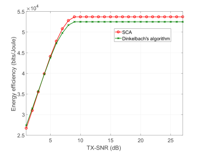
Figure 2: Achieved EE for GEE-Max-based design through Algorithms 1 and 2.

Figure 2 shows the achieved EE for the GEE-Max-based designs with different TX-SNR using the algorithms developed through the SCA and Dinkelbach’s techniques. The performance gap between these two approaches is not significant in terms of the achieved EE. However, the design based on the SCA approach outperforms the latter due to the parametrization of the objective function in the latter. As seen in Figure 2, the achieved EE increases with the available transmit power until it reaches the corresponding maximum green power, where it saturates.
In order to demonstrate the advantages of the proposed GEE-Max-based design, we compare the EE of the proposed design with the existing conventional beamforming designs in the literature, namely, beamforming design for SRM in MISO-NOMA system [19], and maximizing the sum rate in MISO-OMA [45, 46] based on the zero-forcing beamforming designs (ZFBF). As evidenced by results in Figure 3, the GEE-Max based design outperforms the other designs in terms of achieved EE. On the other hand, the EE of the SRM-based designs declines dramatically when the transmit power exceeds the green power. This is particularly the case for the SRM-based designs for both NOMA and OMA (i.e., ZFBF), where these design consume all available power for maximizing the achieved sum rate, as will be seen below.
In order to demonstrate the trade-off between the achieved EE and the sum-rate across different beamforming designs, we evaluate the performance of the proposed schemes in terms of the achieved sum-rate of the overall system. Figure 4 illustrates the achieved sum-rates of different designs against a range of transmit powers. As expected, the SRM-based design shows the same performance as the GEE-Max design up to the green power, and outperforms the GEE-Max scheme when the available transmit power exceeds the green power. The sum-rate of the GEE-Max-based scheme remains constant in this region, where it achieves the maximum EE as shown in Figure 3. On the other hand, the achieved sum rates of both SRM and ZFBF schemes increases with the available transmit power while decreasing their of EE performance (Figure 3).

TABLE II: Power allocations and the achieved SINRs for different GEE-Max designs using the SCA, TX-SNR= 2dB.

Channels	User 1		User 2		User 3
	$\overset{*}{\gamma}_{1}$	$P_{1}$ (W)	$\overset{*}{\gamma}_{2}$	$P_{2}$ (W)	$\overset{*}{\gamma}_{3}$	$P_{3}$ (W)
Channel 1	1.2468	0.9095	0.1848	0.9095	0.1482	1.3507
Channel 2	0.9975	0.8660	0.1535	0.8660	0.1381	1.4378
Channel 3	1.3353	0.9115	0.1789	0.9115	0.1512	1.3082
Channel 4	1.8190	0.9815	0.2485	0.9815	0.1640	1.2068
Channel 5	1.4606	0.9400	0.2098	0.9400	0.1551	1.2898

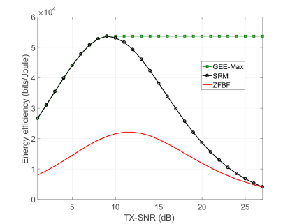
Figure 3: EE for different design criteria.

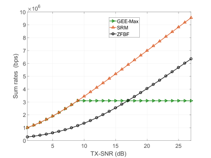
Figure 4: Achieved sum rates of different beamforming designs against transmit power.

To further evaluate the transmit power consumption (i.e., $P_{tr}$), we compare the transmit power requirements for different NOMA beamforming designs. As shown in Figure 5, the P-Min beamforming design [21] outperforms the SRM- and GEE-Max-based designs. This is because the P-Min-based beamforming design uses the transmit power to satisfy the required SINR constraints. On the other hand, the SRM-based scheme makes use of all the available transmit power to achieve the maximum sum rate, while the GEE-Max-based scheme consumes a certain amount of transmit power (i.e., green power) to maximize the GEE of the system. From these observations, the GEE-Max-based design can be considered as the scheme that strikes a good balance between the SRM and P-Min-based designs.

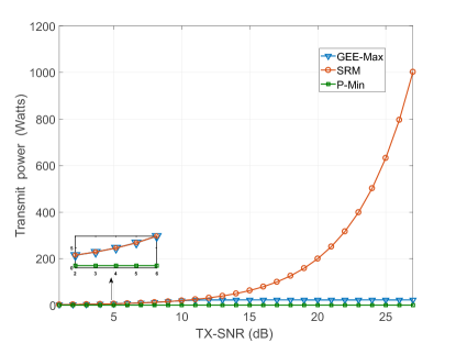
Figure 5: Required transmit power for different beamforming design criteria.

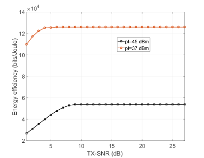
Figure 6: Achieved EE of GEE-Max design with different power losses.

Furthermore, we evaluate the impact of the power losses on the performance of the proposed GEE-Max design. Figure 6 shows the achieved EE against different power losses. There are two key observations to be drawn from Figure 6. Firstly, the achievable EE decreases as the power loss increases. Secondly, the green power that achieves the maximum EE increases as the power losses increases.

TABLE III: Power allocations for the achieved SINRs in Table II using the P-Min design.

Channels	$P_{i}$=Tr[$\mathbf{W}_{i}]$
	$P_{1}$ (W)	$P_{2}$ (W)	$P_{3}$ (W)
Channel 1	0.9094	0.9095	1.3508
Channel 2	0.8660	0.8660	1.4379
Channel 3	0.9113	0.9115	1.3082
Channel 4	0.9815	0.9815	1.2068
Channel 5	0.9400	0.9400	1.2897

Next, we provide results to validate the optimality of the proposed SCA-based GEE-Max algorithm. We compare the achieved SINRs and power allocations of the proposed scheme with the P-Min-based scheme, which assumes to use the same SINR targets obtained in the GEE-Max-based scheme. The power allocations and the achieved SINRs using the proposed SCA- and GEE-Max-based schemes are given for five different random channels in Table II. For the same set of channels used in Table II, the power allocations obtained through solving the P-Min ${\overset{\sim}{OP_{2}}}$ are given in Table III where the achieved SINRs in Table II have been set as the target SINRs in ${\overset{\sim}{OP_{2}}}$. By comparing the results provided in Tables II and III, it can be concluded that both problems provide the same solutions in terms of power allocation. It can also be noticed that the beamforming vectors obtained in both case are the same, and they are not presented here for the reasons of brevity. Therefore, we can confirm that the SCA algorithm yields the optimal solution to the original GEE-Max problem within a few cycles of iterations.

Now, we consider the effect of the path loss exponent $\kappa$ on the achieved EE for the GEE-Max design in Table IV. As expected, the achieved EE decreases as $\kappa$ increases. On the other hand, the base station requires additional transmit power (i.e., $P_{tr}$) to maximize EE when the path loss exponent $\kappa$ increases, as shown in Table IV.

TABLE IV: Achieved EE of the proposed GEE-Max design with different path loss exponents $\kappa$ under TX-SNR= 25 dB.

Path Loss Exponent ($\kappa$)	GEE-Max design
	Achieved EE (Mbits/Joule)	$P_{tr}$ (W)
1	0.0532	22.6202
2	0.0450	24.9749
3	0.0254	64.2730
4	0.0101	287.4765

In addition, Figure 7 illustrates the achieved EE against different number of transmit antennas for the proposed GEE-Max and the SRM designs. In general, the increase in the number of the transmit antennas provides additional degrees of freedom, and hence, improves the achieved sum-rate of the system through efficient interference mitigation [17]. However, the achieved EE shows a different performance behaviour, as the increase of $N$ will also increase $P_{loss}$, accordingly. With the GEE-Max design, two different behaviours can be observed in Figure 7, as follows. First, the achievable EE increases with the number of transmit antennas. This is due to the fact that the rate improvement offered by the additional number of antennas is dominant in achieved EE than the power loss (i.e., the increase of $P_{loss}$ due to the increase of $N$) introduced by those antennas. Hence, the achieved EE increases gradually until it reaches its maximum with $N=3$. Then, the power loss with more number of transmit antennas becomes more dominant in the achieved EE than the rate improvement offered by those antennas. Hence, with more number of antennas, the achieved EE begins to decrease and shows the same performance as in the SRM design as seen in Figure 7. However, the EE achieved through the GEE-Max design outperforms the SRM design. Based on these observations, we can conclude that there is an optimal number of transmit antennas which can achieve the maximum EE and employing a larger number of antennas than the optimal number will introduce a loss in the achievable EE performance of the system. Note that this optimal number of transmit antennas depends on the system parameters (i.e., $K$, $p_{dyn}$, $p_{sta}$, etc.). Furthermore, both the SRM design and GEE-Max design achieve the same EE when the number of transmit antennas is greater than 7. This is due to the fact that the available power (i.e., $P_{ava}$) is less than the green power, hence, both designs will provide the same solution and achieve the same EE performance.

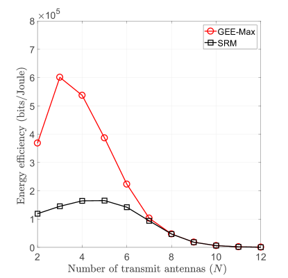
Figure 7: The achieved EE against different number of transmit antenna $N$ for GEE-Max and SRM designs at TX-SNR =10 dB. The $p_{sta}$ and $p_{dyn}$ are set to be 10 dBm and 5 dBm, respectively.

Finally, we evaluate the number of iterations required for the convergence of the proposed SCA-based GEE-Max algorithm. Figure 8 depicts the convergence of the proposed SCA algorithm with different set of channels. The threshold ($\varepsilon$ in Algorithm 1) to terminate the algorithm has been set to 0.01. As seen in Figure 8, the algorithm converges within a few iterations.

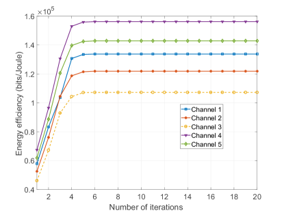
Figure 8: The convergence of SCA based GEE-Max algorithm for different set of random channels. The TX-SNR and $P_{loss}$ are set to be 20 dB and 40 dBm, respectively.

V Conclusions

In this paper, we proposed two different algorithms for energy efficient beamforming designs to maximize the GEE for MISO-NOMA systems. These two algorithms stem from an approach whereby we transformed the original, non-convex GEE-Max optimization problem into an approximated convex problem. The algorithms are based on the sequential convex programming and the Dinkelbach’s approaches, respectively. Our evaluation, benchmarked against a baseline, showed that the proposed algorithms converge and produce similar results, and also outperform the benchmark approaches. Our evaluation also verified the optimality of the proposed SCA-based design by comparing the power allocations with the an equivalent P-Min design with the same set of random channels. Furthermore, it was shown that the GEE-Max based design is capable of achieving a good trade-off between the designs with conflicting performance metrics that maximize the sum rate and minimize the transmit power.

Appendix A

PROOF OF THEOREM 1

To prove Theorem 1, we firstly rewrite (42) such as

$$\chi^{*}=\frac{f_{1}(\{\mathbf{w}^{*}_{i}\}_{i=1}^{K})}{f_{2}(\{\mathbf{w}^{*}_{i}\}_{i=1}^{K})}\geq\frac{f_{1}(\{\mathbf{w}_{i}\}_{i=1}^{K})}{f_{2}(\{\mathbf{w}_{i}\}_{i=1}^{K})},$$ (52)

where $\{\mathbf{w}_{i}^{*}\}_{i=1}^{K}$ denote the beamforming vectors that maximize the original problem $OP_{1}$. Without loss of generality, the condition in (52) can be decomposed as

$$f_{1}(\{\mathbf{w}_{i}\}_{i=1}^{K})-\chi^{*}f_{2}(\{\mathbf{w}_{i}\}_{i=1}^{K})\leq 0,$$ (53a)

$$f_{1}(\{\mathbf{w}^{*}_{i}\}_{i=1}^{K})-\chi^{*}f_{2}(\{\mathbf{w}^{*}_{i}\}_{i=1}^{K})=0,$$ (53b)

where the left side of (53a) denotes the objective function of the parametrized optimization problem $OP_{5}$ (i.e., $F(\{\mathbf{w}_{i}\}_{i=1}^{K},\chi^{*})$). The inequality in (53a) reveals that any feasible beamforming set $\{\mathbf{w}_{i}\}_{i=1}^{K}$ (rather than the optimal set) will provide $F(\{\mathbf{w}_{i}\}_{i=1}^{K},\chi^{*})$ to be less than zero, whereas the optimal beamfroming vectors $\{\mathbf{w}_{i}^{*}\}_{i=1}^{K}$ could be achieved if and only if the condition in (53b) is satisfied. Hence, we can determine the optimal beamforming vectors of the original fractional problem $OP_{1}$ by solving the non-fractional one in $OP_{5}$ with the assumption that the maximum objective value of $OP_{5}$ is zero. This completes the proof of Theorem 1. $\blacksquare$

Appendix B

PROOF OF LEMMA 1

In order to prove the convergence of the Dinkelbach’s iterative approach to the optimal solution, the following conditions can be equivalently proven [37]:

$$\chi^{(n+1)}\geq\chi^{(n)},$$ (54a)

$$\underset{n\rightarrow\infty}{\text{lim}}\chi^{(n)}=\chi^{*}.$$ (54b)

We start with $\chi^{(n+1)}\geq\chi^{(n)}$, and it is known that $F(\chi)$ is a non-decreasing function. Therefore

$$\{F(\chi^{(n)})\geq F(\chi^{*})\geq 0|\chi^{(n)}\leq\chi^{*}\},$$

which implies that

$$f_{1}(\{\mathbf{w}^{(n)}_{i}\}_{i=1}^{K})-\chi^{n}f_{2}(\{\mathbf{w}^{(n)}_{i}\}_{i=1}^{K})\geq 0.$$ (55)

On the other hand, the following holds based on (44):

$$f_{1}(\{\mathbf{w}^{n}_{i}\}_{i=1}^{K})=\chi^{(n+1)}f_{2}(\{\mathbf{w}^{(n)}_{i}\}_{i=1}^{K}).$$ (56)

By substituting (56) in (55), we have:

$$(\chi^{(n+1)}-\chi^{(n)})f_{2}(\{\mathbf{w}^{(n)}_{i}\}_{i=1}^{K})>0.$$

Since $f_{2}(\{\mathbf{w}^{(n)}_{i}\}_{i=1}^{K})$ is assumed to be always positive, then

$$(\chi^{(n+1)}-\chi^{(n)})>0,$$

which confirms the inequality in (54a). Now, we consider the second condition in (54b) and prove this through contradiction. First, we assume that the condition in (54b) does not hold and there exists another non-negative parameter ($\chi^{+}$) such that

$$\underset{n\rightarrow\infty}{\text{lim}}\chi^{(n)}=\chi^{+}<\chi^{*}.$$

Based on this argument, the following holds:

$$F(\chi^{+})=0.$$

However, $F(\chi)$ is a non-decreasing function, which means that

$$\{F(\chi^{+})=0>F(\chi^{*})=0|\chi^{+}<\chi^{*}\},$$ (57)

which is obviously not true and contradicts the assumption made at the beginning of this proof. Therefore,

$$\underset{n\rightarrow\infty}{\text{lim}}\chi^{(n)}=\chi^{*}.$$

This confirms that the Dinkelbach’s iterative algorithm converges to the optimal solution, which completes the proof of Lemma 1. $\blacksquare$

Haitham Moffaqq Al-Obiedollah received the BSc degree from the Electrical Engineering Department, Jordan University of Science and Technology, Jordan in 2006 and Ms.c in communication engineering from Yarmouk University, Jordan in 2012. He is currently pursuing the Ph.D. degree with the Department of Electronics Engineering, the University of York, U.K. He is funded by Hashemite University, Jordan. His current research interests include non-orthogonal multiple access (NOMA), resource allocation techniques, beamforming designs, multi-objective optimization techniques, and convex optimization theory.

Kanapathippillai Cumanan (M’10) received the B.Sc. (Hons.) degree in electrical and electronic engineering from the University of Peradeniya, Sri Lanka, in 2006, and the Ph.D. degree in signal processing for wireless communications from Loughborough University, Loughborough, U.K.,in 2009. He is currently a Lecturer with the Department of Electronics, University of York, U.K. He was with the School of Electronic, Electrical and System Engineering, Loughborough University, U.K. He was a Teaching Assistant with the Department of Electrical and Electronic Engineering, University of Peradeniya, Sri Lanka, in 2006. In 2011, he was an Academic Visitor with the Department of Electrical and Computer Engineering, National University of Singapore, Singapore. He was a Research Associate with the School of Electrical and Electronic Engineering, Newcastle University, U.K., from 2012 to 2014. His research interests include physical layer security, cognitive radio networks, relay networks, convex optimization techniques, and resource allocation techniques. Dr. Cumanan was a recipient of an Overseas Research Student Award Scheme from Cardiff University, Wales, U.K., where he was a Research Student from 2006 to 2007.

Jeyarajan Thiyagalingam received his PhD degree in Computer Science from Imperial College, London, in 2005. Currently, he is a Senior Scientist at the Science and Technologies Facilities Council, Rutherford Appleton Laboratory (STFC-RAL) in Harwell, Oxford, UK. Before joining STFC-RAL, he was an academic at the University of Liverpool, and previously held positions at MathWorks UK and at the University of Oxford. His research interests include computationally efficient algorithms and models for machine learning systems, machine learning models for signal processing applications, such as target tracking, estimation, and application of machine learning for fundamental science. He is a Fellow of the British Computer Society and also a member of IET and IEEE.

Alister Burr was born in London, U.K, in 1957. He received the BSc degree in Electronic Engineering from the University of Southampton, U.K in 1979 and the PhD from the University of Bristol in 1984. Between 1975 and 1985 he worked at Thorn-EMI Central Research Laboratories in London. In 1985 he joined the Department of Electronics (now Electronic Engineering) at the University of York, U.K, where he has been Professor of Communications since 2000. His research interests are in wireless communication systems, especially MIMO, cooperative systems, physical layer network coding, and iterative detection and decoding techniques. He has published around 250 papers in refereed international conferences and journals, and is the author of “Modulation and Coding for Wireless Communications” (published by Prentice-Hall/PHEI), and co-author of “Wireless Physical-Layer Network Coding (Cambridge University Press, 2018). In 1999 he was awarded a Senior Research Fellowship by the U.K. Royal Society, and in 2002 he received the J. Langham Thompson Premium from the Institution of Electrical Engineers. He has also given more than 15 invited presentations, including three keynote presentations. He was chair, working group 2, of a series of European COST programmes including IC1004 “Cooperative Radio Communications for Green Smart Environments” (which have been influential in 3GPP standardisation), and has also served as Associate Editor for IEEE Communications Letters, Workshops Chair for IEEE ICC 2016, and TPC co-chair for PIMRC 2018.

Zhiguo Ding (S’03-M’05) received his B.Eng in Electrical Engineering from the Beijing University of Posts and Telecommunications in 2000, and the Ph.D degree in Electrical Engineering from Imperial College London in 2005. From Jul. 2005 to Apr. 2018, he was working in Queen’s University Belfast, Imperial College, Newcastle University and Lancaster University. Since Apr. 2018, he has been with the University of Manchester as a Professor in Communications. From Oct. 2012 to Sept. 2018, he has also been an academic visitor in Princeton University. Dr Ding’ research interests are 5G networks, game theory, cooperative and energy harvesting networks and statistical signal processing. He is serving as an Editor for IEEE Transactions on Communications, IEEE Transactions on Vehicular Technology, and Journal of Wireless Communications and Mobile Computing, and was an Editor for IEEE Wireless Communication Letters, IEEE Communication Letters from 2013 to 2016. He received the best paper award in IET ICWMC-2009 and IEEE WCSP-2014, the EU Marie Curie Fellowship 2012-2014, the Top IEEE TVT Editor 2017, IEEE Heinrich Hertz Award 2018, the IEEE Jack Neubauer Memorial Award 2018 and the IEEE Best Signal Processing Letter Award 2018.

Octavia A. Dobre (M’05–SM’07) received the Dipl. Ing. and Ph.D. degrees from Politehnica University of Bucharest (formerly Polytechnic Institute of Bucharest), Romania, in 1991 and 2000, respectively. Between 2002 and 2005, she was with Politehnica University of Bucharest and New Jersey Institute of Technology, USA. In 2005, she joined Memorial University, Canada, where she is currently Professor and Research Chair. She was a Visiting Professor with Université de Bretagne Occidentale, France, and Massachusetts Institute of Technology, USA, in 2013. Her research interests include 5G enabling technologies, blind signal identification and parameter estimation techniques, as well as optical and underwater communications. She co-authored more than 250 papers in these areas. Dr. Dobre serves as the Editor-in-Chief of the IEEE COMMUNICATIONS LETTERS, as well as an Editor of the IEEE COMMUNICATIONS SURVEYS AND TUTORIALS and IEEE SYSTEMS. She was an Editor, Senior Editor, and Guest Editor for other prestigious journals. She served as General Chair, Tutorial Co-Chair, and Technical Co-Chair at numerous conferences. Dr. Dobre was a Royal Society Scholar in 2000 and a Fulbright Scholar in 2001. She is a Fellow of the Engineering Institute of Canada.

References

- [1] Y. Saito, Y. Kishiyama, A. Benjebbour, T. Nakamura, A. Li, and K. Higuchi, “Non-orthogonal multiple access (NOMA) for cellular future radio access,” in Proc. IEEE VTC Spring 2013, pp. 1–5.
- [2] S. R. Islam, N. Avazov, O. A. Dobre, and K.-S. Kwak, “Power-domain non-orthogonal multiple access (NOMA) in 5G systems: potentials and challenges,” Commun. Surveys Tuts., vol. 19, no. 2, pp. 721–742, Oct. 2017.
- [3] A. Benjebbour, Y. Saito, Y. Kishiyama, A. Li, A. Harada, and T. Nakamura, “Concept and practical considerations of non-orthogonal multiple access (NOMA) for future radio access,” in Proc. IEEE Intell. Signal Process. and Commun. Syst. (ISPACS), 2013, pp. 770–774.
- [4] S. Tomida and K. Higuchi, “Non-orthogonal access with SIC in cellular downlink for user fairness enhancement,” in Proc. IEEE Inter. Symp. on Intell. Signal Process. and Comm. Sys. (ISPACS), 2011, pp. 1–6.
- [5] S. Vanka, S. Srinivasa, Z. Gong, P. Vizi, K. Stamatiou, and M. Haenggi, “Superposition coding strategies: Design and experimental evaluation,” IEEE Trans. Wireless Commun., vol. 11, no. 7, pp. 2628–2639, Jul. 2012.
- [6] P. Xu and K. Cumanan, “Optimal power allocation scheme for non-orthogonal multiple access with -fairness,” IEEE J. Sel. Areas in Commun., vol. 35, no. 10, pp. 2357–2369, Oct. 2017.
- [7] Z. Zhang, Z. Ma, X. Lei, M. Xiao, C.-X. Wang, and P. Fan, “Power domain non-orthogonal transmission for cellular mobile broadcasting: Basic scheme, system design, and coverage performance,” IEEE Wireless Commun., vol. 25, no. 2, pp. 90–99, Apr. 2018.
- [8] Z. Ding, F. Adachi, and H. V. Poor, “The application of MIMO to non-orthogonal multiple access,” IEEE Trans. Wireless Commun., vol. 15, no. 1, pp. 537–552, Jan. 2016.
- [9] L. Atzori, A. Iera, and G. Morabito, “The Internet of Things: A survey,” Comput. Netw., vol. 54, no. 15, pp. 2787–2805, Oct. 2010.
- [10] B. Wang, L. Dai, Z. Wang, N. Ge, and S. Zhou, “Spectrum and energy-efficient beamspace MIMO-NOMA for millimeter-wave communications using lens antenna array,” IEEE J. Sel. Areas Commun., vol. 35, no. 10, pp. 2370–2382, Oct. 2017.
- [11] Z. Wei, L. Zhao, J. Guo, D. W. K. Ng, and J. Yuan, “A multi-beam NOMA framework for hybrid mmwave systems,” in Proc. IEEE International Conference on Communications (ICC) 2018, pp. 1–7.
- [12] Z. Ding, Y. Liu, J. Choi, Q. Sun, M. Elkashlan, and H. V. Poor, “Application of non-orthogonal multiple access in LTE and 5G networks,” IEEE Commun. Mag., vol. 55, no. 2, pp. 185–191, Feb. 2017.
- [13] Q. Sun, S. Han, I. Chin-Lin, and Z. Pan, “On the ergodic capacity of MIMO NOMA systems,” IEEE Wireless Commun. Lett., vol. 4, no. 4, pp. 405–408, Aug. 2015.
- [14] L. Lv, J. Chen, and Q. Ni, “Cooperative non-orthogonal multiple access in cognitive radio,” IEEE Commun. Lett., vol. 20, no. 10, pp. 2059–2062, Oct. 2016.
- [15] R. Vannithamby and S. Talwar, Towards 5G Applications: Requirements and Candidate Technologies. John Wiley & Sons, 2017.
- [16] P. Gandotra, R. K. Jha, and S. Jain, “Green communication in next generation cellular networks: a survey,” IEEE Access, vol. 5, pp. 11 727–11 758, Jun. 2017.
- [17] O. Tervo, L.-N. Tran, and M. Juntti, “Optimal energy-efficient transmit beamforming for multi-user MISO downlink,” IEEE Trans. Signal Process., vol. 63, no. 20, pp. 5574–5588, Oct. 2015.
- [18] A. Zappone and E. Jorswieck, “Energy efficiency in wireless networks via fractional programming theory,” Found. Trends Commun. Inf. Theory, vol. 11, no. 3-4, pp. 185–396, Jan. 2015.
- [19] M. F. Hanif, Z. Ding, T. Ratnarajah, and G. K. Karagiannidis, “A minorization-maximization method for optimizing sum rate in the downlink of non-orthogonal multiple access systems,” IEEE Trans. Signal Process., vol. 64, no. 1, pp. 76–88, Jan. 2016.
- [20] D. R. Hunter and K. Lange, “A tutorial on MM algorithms,” Amer. Statistician, vol. 58, no. 1, pp. 30–37, 2004.
- [21] Z. Chen, Z. Ding, P. Xu, and X. Dai, “Optimal precoding for a QoS optimization problem in two-user MISO-NOMA downlink,” IEEE Commun. Lett., vol. 20, no. 6, pp. 1263–1266, Jun. 2016.
- [22] Y. Zhang, H.-M. Wang, T.-X. Zheng, and Q. Yang, “Energy-efficient transmission design in non-orthogonal multiple access,” IEEE Trans. Veh. Technol., vol. 66, no. 3, pp. 2852–2857, Mar. 2017.
- [23] S. Boyd and L. Vandenberghe, Convex Optimization. Cambridge Univ. Press, 2004.
- [24] F. Fang, H. Zhang, J. Cheng, and V. C. Leung, “Energy-efficient resource allocation for downlink non-orthogonal multiple access network,” ” IEEE Trans. Commun., vol. 64, no. 9, pp. 3722–3732, Sep. 2016.
- [25] J. Zhu, J. Wang, Y. Huang, S. He, X. You, and L. Yang, “On optimal power allocation for downlink non-orthogonal multiple access systems,” IEEE J. Sel. Areas Commun., vol. 35, no. 12, pp. 2744–2757, Dec. 2017.
- [26] M. Zeng, A. Yadav, O. A. Dobre, and H. V. Poor, “Energy-efficient power allocation for mimo-noma with multiple users in a cluster,” IEEE Access, vol. 6, pp. 5170–5181, Feb. 2018.
- [27] S. Islam, M. Zeng, O. A. Dobre, and K.-S. Kwak, “Resource allocation for downlink noma systems: Key techniques and open issues,” IEEE Wireless Commun., vol. 25, no. 2, pp. 40–47, Apr. 2018.
- [28] L. Wang, M. Guan, Y. Ai, Y. Chen, B. Jiao, and L. Hanzo, “Beamforming aided NOMA expedites collaborative multiuser computational off-loading,” IEEE Trans. Veh. Technol., vol. 67, no. 10, pp. 10 027–10 032, Oct. 2018.
- [29] F. Fang, H. Zhang, J. Cheng, S. Roy, and V. C. Leung, “Joint user scheduling and power allocation optimization for energy efficient NOMA systems with imperfect CSI,” IEEE J. Sel. Areas Commun, vol. 35, no. 12, pp. 2874–2885, Dec. 2017.
- [30] K. Cumanan, R. Krishna, L. Musavian, and S. Lambotharan, “Joint beamforming and user maximization techniques for cognitive radio networks based on branch and bound method,” IEEE Trans. Wireless Commun., vol. 9, no. 10, pp. 3082–3092, Oct. 2010.
- [31] P. Xu, K. Cumanan, and Z. Yang, “Optimal power allocation scheme for noma with adaptive rates and alpha-fairness,” in Proc. IEEE GLOBECOM, 2017, pp. 1–6.
- [32] H. Alobiedollah, K. Cumanan, J. Thiyagalingam, A. G. Burr, Z. Ding, and O. A. Dobre, “Energy efficiency fairness beamforming design for MISO NOMA systems,” in Proc. IEEE WCNC, 2019.
- [33] ——, “Sum rate fairness trade-off-based resource allocation technique for MISO NOMA systems,” in Proc. IEEE WCNC, 2019.
- [34] A. Beck, A. Ben-Tal, and L. Tetruashvili, “A sequential parametric convex approximation method with applications to nonconvex truss topology design problems,” J. Global Optimiz., vol. 47, no. 1, pp. 29–51, May 2010.
- [35] Z.-Q. Luo and W. Yu, “An introduction to convex optimization for communications and signal processing,” IEEE J. Sel. Areas Commun., vol. 24, no. 8, pp. 1426–1438, Aug. 2006.
- [36] F. Alavi, K. Cumanan, Z. Ding, and A. G. Burr, “Beamforming techniques for non-orthogonal multiple access in 5G cellular networks,” IEEE Trans. Veh. Technol., vol. 67, no. 10, pp. 9474–9487, Oct. 2018.
- [37] W. Dinkelbach, “On non linear fractional programming,” Manage. Sci., vol. 13, no. 7, pp. 492–498, Mar. 1967.
- [38] M. Bengtsson and B. Ottersten, “Optimal downlink beamforming using semidefinite optimization,” in Proc. Annual Allerton Conf. on Commun., Control and Computing, 1999, pp. 987–996.
- [39] K. Cumanan, R. Krishna, V. Sharma, and S. Lambotharan, “Robust interference control techniques for multiuser cognitive radios using worst-case performance optimization,” in Proc. IEEE Asilomar Conf. Signal, Syst. Comput., 2008, pp. 378–382.
- [40] F. Alavi, K. Cumanan, Z. Ding, and A. G. Burr, “Robust beamforming techniques for non-orthogonal multiple access systems with bounded channel uncertainties,” IEEE Commun. Lett., vol. 21, no. 9, pp. 2033–2036, Sept. 2017.
- [41] K. Cumanan, R. Krishna, Z. Xiong, and S. Lambotharan, “SINR balancing technique and its comparison to semidefinite programming based qos provision for cognitive radios,” in Proc. IEEE VTC Spring, 2009, pp. 1–5.
- [42] Y. Nesterov and A. Nemirovskii, Interior-point Polynomial Algorithms in Convex Programming. Philadelphia, PA: SIAM, 1994.
- [43] M. S. Lobo, L. Vandenberghe, S. Boyd, and H. Lebret, “Applications of second-order cone programming,” Linear Algebra and its Appl., vol. 284, pp. 193–228, Nov. 1998.
- [44] M. Grant, S. Boyd, and Y. Ye, “CVX: Matlab software for disciplined convex programming,” 2008.
- [45] C. Peel, Q. Spencer, A. L. Swindlehurst, and B. Hochwald, “Downlink transmit beamforming in multi-user MIMO systems,” in Proc. Sensor Array Multichannel Signal Process. Workshop, Jul. 2004, pp. 43–51.
- [46] A. Wiesel, Y. C. Eldar, and S. Shamai, “Zero-forcing precoding and generalized inverses,” IEEE Trans. Signal Process., vol. 56, no. 9, pp. 4409–4418, Sep. 2008.