Anisotropic $\boldsymbol{2}$-form dark energy

Abstract

We study the dynamics of dark energy in the presence of a 2-form field coupled to a canonical scalar field $\phi$. We consider the coupling proportional to $e^{-\mu\phi/M_{\rm pl}}H_{\alpha\beta\gamma}H^{\alpha\beta\gamma}$ and the scalar potential $V(\phi)\propto e^{-\lambda\phi/M_{\rm pl}}$, where $H_{\alpha\beta\gamma}$ is the 2-form field strength, $\mu,\lambda$ are constants, and $M_{\rm pl}$ is the reduced Planck mass. We show the existence of an anisotropic matter-dominated scaling solution followed by a stable accelerated fixed point with a non-vanishing shear. Even if $\lambda\geq{\cal O}(1)$, it is possible to realize the dark energy equation of state $w_{\rm DE}$ close to $-1$ at low redshifts for $\mu\gg\lambda$. The existence of anisotropic hair and the oscillating behavior of $w_{\rm DE}$ are key features for distinguishing our scenario from other dark energy models like quintessence.

I Introduction

Since the first discovery of late-time cosmic acceleration from the distant supernovae type Ia (SN Ia) SN1 ; SN2 , the origin of this phenomenon has not been identified yet. The cosmological constant is a simplest candidate for dark energy, but if it originates from vacuum energy associated with particle physics, it is plagued by a huge energy gap between its observed value and the theoretically predicted value Weinberg . Instead, there are dynamical dark energy models dubbed quintessence in which a canonical scalar field $\phi$ slowly evolving along a potential $V(\phi)$ leads to a time-varying field equation of state quin1 ; quin2 ; quin3 ; quin4 ; quin5 ; quin6 ; quin7 .

In quintessence, the condition for cosmic acceleration can be quantified by the dimensionless parameter $\lambda=-M_{\rm pl}V_{,\phi}/V$, where $M_{\rm pl}$ is the reduced Planck mass and $V_{,\phi}={\rm d}V/{\rm d}\phi$. For constant $\lambda$, i.e., for the exponential potential $V(\phi)=V_{0}e^{-\lambda\phi/M_{\rm pl}}$, the accelerated expansion occurs for $|\lambda|<\sqrt{2}$ CLW ; CST ; Tsuji13 . Under this condition, the solutions finally approach an attractor characterized by the dark energy equation of state $w_{\rm DE}=-1+\lambda^{2}/3$.

In the context of higher-dimensional theories like string/M theories, the exponential potential can arise from compactifications in hyperbolic manifolds or S-brane solutions Garriga:2000cv ; Emparan:2003gg . After the dimensional reduction, the slope $|\lambda|$ is typically larger than the order 1. In this case the accelerated attractor mentioned above is not present, while the temporal cosmic acceleration is possible for the internal manifold changing in time Townsend:2003fx ; Ohta:2003pu ; Wohlfarth:2003ni ; Roy:2003nd . The construction of a meta-stable de Sitter vacuum in string theory also suggested the swampland conjecture stating that $|\lambda|$ has a lower bound of order 1 swamp1 ; swamp2 . It is worthy of pursuing possibilities for realizing the cosmic acceleration even for steep scalar potentials satisfying $|\lambda|\geq{\cal O}(1)$.

In string theory, there are $p$-form fields arising from the Ramond-Ramond sector string . The 1-form field, which corresponds to a vector field $A_{\mu}$, can be generally coupled to a scalar (0-form) field $\phi$ Almeida:2018fwe . The commonly studied coupling in the cosmological context has the form $-f_{1}(\phi)F_{\mu\nu}F^{\mu\nu}/4$, where $f_{1}(\phi)$ is a function of $\phi$ and $F_{\mu\nu}=\partial_{\mu}A_{\nu}-\partial_{\nu}A_{\mu}$ is the field strength tensor Ratra1991bn ; Bamba2003av ; Martin2007ue ; Yokoyama2008xw ; Dimopoulos2009am ; Dimopoulos2009vu ; Fujita:2018zbr . During the inflationary period, it is known that the vector field can generate the non-vanishing anisotropic shear for a suitable choice of the coupling $f_{1}(\phi)$ related to the scalar potential $V(\phi)$ Watanabe ; Watanabe2 ; Kanno:2010nr ; Ohashi:2013pca . The anisotropic hair sustained during inflation can leave several interesting observational signatures for the 2-point and 3-point correlation functions of Cosmic Microwave Background (CMB) temperature anisotropies Gumrukcuoglu2010yc ; Gum ; Himmetoglu2009mk ; Bartolo ; Namba2012gg ; Shiraishi2013vja ; Fujita2013pgp .

The 2-form field $B_{\alpha\beta}$ coupled to the scalar field $\phi$ through the form $-f_{2}(\phi)H_{\alpha\beta\gamma}H^{\alpha\beta\gamma}/12$, where $f_{2}(\phi)$ is a function of $\phi$ and $H_{\alpha\beta\gamma}$ is the field strength of $B_{\alpha\beta}$, can also give rise to anisotropic inflation for an appropriate choice of $f_{2}(\phi)$ Ohashi2 ; Ito ; Obata:2018ilf ; Almeida:2019xzt . The observational signatures in CMB imprinted by the 2-form is different from those by the 1-form, so they can be distinguished between each other from the scalar power spectrum and primordial non-Gaussianities Ohashi:2013qba . If the anisotropic shear does not survive either during inflation or in the later cosmological epoch, the 2-form energy density decreases as $\rho_{B}\propto a^{-2}$, where $a$ is the isotropic scale factor. This is in contrast to the 1-form field, whose energy density decreases as radiation ($\rho_{A}\propto a^{-4}$) in the isotropic context. Hence the energy density of 2-form can be generally prominent at late times compared to that of 1-form.

For the 1-form field coupled to a dark energy field $\phi$, Thorsrud et al. Thorsrud:2012mu studied the late-time cosmological dynamics in the presence of an additional coupling between $\phi$ and matter. They found interesting anisotropic scaling solutions relevant to the matter and dark energy dominated epochs. The existence of non-vanishing anisotropic shear after the decoupling epoch leaves modifications to the observables in CMB and SN Ia measurements Koivisto:2007bp ; Koivisto:2008ig ; Battye:2009ze ; Appleby:2009za ; Campanelli:2010zx ; Appleby:2012as .

In this paper, we study the late-time cosmology in the presence of the interaction $-f(\phi)H_{\alpha\beta\gamma}H^{\alpha\beta\gamma}/12$ between the 2-form and the scalar field $\phi$. We consider the exponential potential $V(\phi)=V_{0}e^{-\lambda\phi/M_{\rm pl}}$ for the scalar sector and adopt the coupling of the form $f(\phi)=f_{0}e^{-\mu\phi/M_{\rm pl}}$. We show that, even for $\lambda\geq{\cal O}(1)$, the late-time cosmic acceleration with the dark energy equation of state $w_{\rm DE}$ close to $-1$ can be realized for the coupling constant $\mu$ in the range $\mu\gg\lambda$. Thus, this model is an explicit example where the accelerated expansion consistent with current observations Betoule:2014frx ; Aghanim:2018eyx is possible even with a steep exponential potential.

Moreover, we show that the radiation-dominated epoch with an initially negligible anisotropic shear is followed by the scaling matter era with a non-vanishing anisotropic hair. As long as the anisotropic dark energy dominated fixed point is present, it is a stable spiral for $\mu\gg\lambda\geq{\cal O}(1)$. Thus, our model gives rise to several interesting observational signatures such as the surviving anisotropic shear after the radiation era and the oscillating dark energy equation of state in the range $w_{\rm DE}>-1$.

This paper is organized as follows. In Sec. II, we derive the background equations of motion in the presence of a perfect fluid on the anisotropic cosmological background. In Sec. III, we obtain the fixed points associated with radiation, matter, and dark energy dominated epochs and discuss the stabilities of them. In Sec. IV, we study the cosmological dynamics in our model by paying particular attention to the evolution of $w_{\rm DE}$ and the anisotropic shear. Finally, Sec. V is devoted to conclusions. Throughout the paper, we use the Lorentzian metric $g_{\mu\nu}$ with the sign convention $(-,+,+,+)$, and greek indices as $\alpha,\beta,\gamma\cdots$, will denote space-time coordinates.

II Background equations of motion

In the 4-dimensional space-time, we consider a 2-form field $B_{\alpha\beta}$ with the field strength $H_{\alpha\beta\gamma}=3\partial_{[\alpha}B_{\beta\gamma]}$. We also take into account a canonical scalar field $\phi$ with the potential $V(\phi)$ and assume that $\phi$ is coupled to the 2-form through the interacting Lagrangian $-f(\phi)H_{\alpha\beta\gamma}H^{\alpha\beta\gamma}/12$. We do not consider non-minimal couplings to gravity, so the gravity sector is described by the Einstein-Hilbert Lagrangian $M_{\rm pl}^{2}R/2$, where $R$ is the Ricci scalar. We also add a perfect fluid described by the purely k-essence Lagrangian $P_{f}(Z)$, where $Z=-\partial_{\mu}\chi\partial^{\mu}\chi/2$ is the kinetic term of a scalar field $\chi$ Hu05 ; Arroja ; KT14 . Then, the action of our theory is given by

$$\mathcal{S} = \int\mathrm{d}^{4}x\sqrt{-g}\biggl{[}\frac{M_{\rm{pl}}^{2}}{2}R-\frac{1}{2}\partial_{\mu}\phi\partial^{\mu}\phi-V(\phi)$$ (1)

$$\qquad\qquad\qquad-\frac{1}{12}f(\phi)H_{\alpha\beta\gamma}H^{\alpha\beta\gamma}+P_{f}(Z)\biggr{]}\,,$$

where $g$ is the determinant of metric tensor $g_{\mu\nu}$ and $f(\phi)$ is a function of $\phi$.

Let us derive the dynamical equations of motion for the action (1) on the anisotropic cosmological background. We consider the configuration in which the 2-form field is in the $(y,z)$ plane, such that

$$B_{\alpha\beta}\mathrm{d}x^{\alpha}\wedge\mathrm{d}x^{\beta}=2v_{B}(t)\mathrm{d}y\wedge\mathrm{d}z\,,$$ (2)

where $v_{B}$ depends on the cosmic time $t$. In the $(y,z)$ plane there is a rotational symmetry, so the line element can be taken as

$$\mathrm{d}s^{2}=-N(t)^{2}\mathrm{d}t^{2}+e^{2\alpha(t)}\left[e^{-4\sigma(t)}\mathrm{d}x^{2}+e^{2\sigma(t)}(\mathrm{d}y^{2}+\mathrm{d}z^{2})\right],$$ (3)

where $N(t)$ is the lapse function, $a\equiv e^{\alpha(t)}$ is the geometric mean of three scale factors (with the normalization $a=1$ today), and $\sigma(t)$ is the spatial shear. The non-vanishing components of $B_{\alpha\beta}$ are $B_{23}=-B_{32}=v_{B}$. On the background (3), the action (1) is expressed as

$${\cal S} = \int{\rm d}^{4}x\biggl{[}\frac{3M_{\rm pl}^{2}e^{3\alpha}}{N}\left(\dot{\sigma}^{2}-\dot{\alpha}^{2}\right)+e^{3\alpha}\left\{\frac{\dot{\phi}^{2}}{2N}-NV(\phi)\right\}$$ (4)

$$\qquad\quad+\frac{f(\phi)}{2N}e^{-\alpha-4\sigma}\dot{v}_{B}^{2}+Ne^{3\alpha}P_{f}(Z(N))\biggr{]},$$

where $Z=\dot{\chi}^{2}/(2N^{2})$ and a dot represents a derivative with respect to $t$.

Varying the action (4) with respect to $N,\alpha,\sigma,\phi$, $\chi$ and setting $N=1$ at the end, we obtain

$$3M_{\rm pl}^{2}H^{2}\left(1-\Sigma^{2}\right)=\frac{1}{2}\dot{\phi}^{2}+V(\phi)+\rho_{B}+\rho_{f}\,,$$ (5)

$$M_{\rm pl}^{2}\left(\dot{H}+3H^{2}\Sigma^{2}\right)=-\frac{1}{2}\dot{\phi}^{2}-\frac{1}{3}\rho_{B}-\frac{1}{2}\left(\rho_{f}+P_{f}\right),$$ (6)

$$M_{\rm pl}^{2}\left[H\dot{\Sigma}+\left(\dot{H}+3H^{2}\right)\Sigma\right]=-\frac{2}{3}\rho_{B}\,,$$ (7)

$$\ddot{\phi}+3H\dot{\phi}+V_{,\phi}-\frac{f_{,\phi}}{f}\rho_{B}=0\,,$$ (8)

$$\dot{\rho}_{f}+3H\left(\rho_{f}+P_{f}\right)=0\,,$$ (9)

being

$$H\equiv\dot{\alpha}\,,\qquad\Sigma\equiv\frac{\dot{\sigma}}{H}\,,$$ (10)

and $\rho_{B}$ and $\rho_{f}$ correspond to the energy densities of the 2-form and the perfect fluid, defined, respectively, by

$$\rho_{B}=\frac{f(\phi)}{2}e^{-4\alpha-4\sigma}\dot{v}_{B}^{2}\,,\qquad\rho_{f}=\dot{\chi}^{2}P_{f,Z}-P_{f}\,.$$ (11)

Note that we used the notation in which a comma in the subscript represents a derivative with respect to a corresponding variable, e.g., $f_{,\phi}={\rm d}f/{\rm d}\phi$. Varying the action (4) with respect to $v_{B}$, it follows that

$$f(\phi)e^{-\alpha-4\sigma}\dot{v}_{B}=p_{B}\,,$$ (12)

where $p_{B}$ is a constant. Taking the time derivative of $\rho_{B}$ in Eq. (11) and using Eq. (12), the 2-form energy density $\rho_{B}$ obeys the differential equation,

$$\dot{\rho}_{B}=-2H\rho_{B}\left(1-2\Sigma+\frac{\dot{f}}{2Hf}\right)\,.$$ (13)

For the scalar potential $V(\phi)$ and the coupling $f(\phi)$, we adopt the exponential functions given by Ito ; Kanno:2010nr ; Ohashi:2013pca :

$$V(\phi)=V_{0}e^{-\lambda\phi/M_{\rm pl}}\,,\qquad f(\phi)=f_{0}e^{-\mu\phi/M_{\rm pl}}\,,$$ (14)

where $V_{0},\lambda,f_{0},\mu$ are assumed to be positive constants. We are interested in the case in which the late-time cosmic acceleration can be realized for

$$\lambda\geq{\cal O}(1)\,,\qquad\mu\geq{\cal O}(1)\,,$$ (15)

whose conditions are assumed in the following. If the coupling $f(\phi)$ is absent, the cosmic acceleration with the dark energy equation of state close to $-1$ occurs only for $\lambda^{2}\ll 2$ CLW ; CST ; Tsuji13 .

III Dynamical system and fixed points

We express the background equations of motion derived in Sec. II in an autonomous form and obtain the corresponding fixed points. For the perfect fluid given by the Lagrangian $P_{f}(Z)$, we take into account both non-relativistic matter (energy density $\rho_{m}$ and negligible pressure) and radiation (energy density $\rho_{r}$ and pressure $P_{r}=\rho_{r}/3$), so that $\rho_{f}=\rho_{m}+\rho_{r}$ and $P_{f}=\rho_{r}/3$.

III.1 Dynamical system

We introduce the following dimensionless quantities:

$$x_{1}=\frac{\dot{\phi}}{\sqrt{6}HM_{\rm pl}}\,,\quad x_{2}=\frac{\sqrt{V}}{\sqrt{3}HM_{\rm pl}}\,,\quad\Omega_{B}=\frac{\rho_{B}}{3H^{2}M_{\rm pl}^{2}}\,,$$

$$\Omega_{r}=\frac{\rho_{r}}{3H^{2}M_{\rm pl}^{2}}\,,\quad\Omega_{m}=\frac{\rho_{m}}{3H^{2}M_{\rm pl}^{2}}\,.$$ (16)

From Eq. (5), there is the constraint

$$\Omega_{m}=1-x_{1}^{2}-x_{2}^{2}-\Sigma^{2}-\Omega_{B}-\Omega_{r}\,.$$ (17)

By using Eqs. (6) and (8) with Eq. (17), we obtain

$$\frac{\dot{H}}{H^{2}} = -\frac{1}{2}\left(3+3x_{1}^{2}-3x_{2}^{2}+3\Sigma^{2}-\Omega_{B}+\Omega_{r}\right)\,,$$ (18)

$$\frac{\ddot{\phi}}{H\dot{\phi}} = -3+\frac{\sqrt{6}}{2x_{1}}\left(\lambda x_{2}^{2}-\mu\Omega_{B}\right)\,.$$ (19)

From Eqs. (7), (9), (17), (18), and (19), the dimensionless variables $x_{1},x_{2},\Sigma,\Omega_{B}$, and $\Omega_{r}$ obey

$$x_{1}^{\prime} = \frac{3}{2}x_{1}\left(x_{1}^{2}-x_{2}^{2}+\Sigma^{2}-1-\frac{1}{3}\Omega_{B}+\frac{1}{3}\Omega_{r}\right)$$ (20)

$$+\frac{\sqrt{6}}{2}\left(\lambda x_{2}^{2}-\mu\Omega_{B}\right)\,,$$

$$x_{2}^{\prime} = \frac{1}{2}x_{2}(3x_{1}^{2}-3x_{2}^{2}+3\Sigma^{2}+3-\sqrt{6}\lambda x_{1}$$ (21)

$$-\Omega_{B}+\Omega_{r})\,,$$

$$\Sigma^{\prime} = \frac{1}{2}\Sigma\left(3x_{1}^{2}-3x_{2}^{2}+3\Sigma^{2}-3-\Omega_{B}+\Omega_{r}\right)$$ (22)

$$-2\Omega_{B}\,,$$

$$\Omega_{B}^{\prime} = \Omega_{B}(3x_{1}^{2}-3x_{2}^{2}+3\Sigma^{2}+4\Sigma+1+\sqrt{6}\mu x_{1}$$ (23)

$$-\Omega_{B}+\Omega_{r})\,,$$

$$\Omega_{r}^{\prime} = \Omega_{r}\left(3x_{1}^{2}-3x_{2}^{2}+3\Sigma^{2}-1-\Omega_{B}+\Omega_{r}\right)\,,$$ (24)

where a prime represents a derivative with respect to the number of e-foldings $\alpha=\ln a$. The cosmological dynamics is known by solving Eqs. (20)-(24) with Eq. (17) for given initial values of $x_{1},x_{2},\Sigma,\Omega_{B},\Omega_{r}$.

The effective equation of state, which is defined by $w_{\rm eff}\equiv-1-2\dot{H}/(3H^{2})$, characterizes the evolution of mean scale factor $a(t)$. From Eq. (18), it follows that

$$w_{\rm eff}=x_{1}^{2}-x_{2}^{2}+\Sigma^{2}-\frac{1}{3}\Omega_{B}+\frac{1}{3}\Omega_{r}\,.$$ (25)

The radiation- and matter-dominated epochs correspond to $w_{\rm eff}\simeq 1/3$ and $w_{\rm eff}\simeq 0$, respectively. The cosmic acceleration occurs for $w_{\rm eff}<-1/3$. We can express Eqs. (5) and (6) in the form:

$$3M_{\rm pl}^{2}H^{2}=\rho_{\rm DE}+\rho_{r}+\rho_{m}\,,$$ (26)

$$2M_{\rm pl}^{2}\dot{H}=-\rho_{\rm DE}-P_{\rm DE}-\frac{4}{3}\rho_{r}-\rho_{m}\,,$$ (27)

where

$$\rho_{\rm DE} = \frac{1}{2}\dot{\phi}^{2}+V(\phi)+\rho_{B}+3M_{\rm pl}^{2}H^{2}\Sigma^{2}\,,$$ (28)

$$P_{\rm DE} = \frac{1}{2}\dot{\phi}^{2}-V(\phi)-\frac{1}{3}\rho_{B}+3M_{\rm pl}^{2}H^{2}\Sigma^{2}\,.$$ (29)

Defining the density parameter and the equation of state arising from the dark sector, as $\Omega_{\rm DE}=\rho_{\rm DE}/(3H^{2}M_{\rm pl}^{2})$ and $w_{\rm DE}=P_{\rm DE}/\rho_{\rm DE}$, respectively, it follows that

$$\Omega_{\rm DE} = x_{1}^{2}+x_{2}^{2}+\Sigma^{2}+\Omega_{B}=1-\Omega_{r}-\Omega_{m}\,,$$ (30)

$$w_{\rm DE} = \frac{3(x_{1}^{2}-x_{2}^{2}+\Sigma^{2})-\Omega_{B}}{3(x_{1}^{2}+x_{2}^{2}+\Sigma^{2}+\Omega_{B})}\,,$$ (31)

where we used Eq. (17) in the second equality of Eq. (30). The above definitions of $\Omega_{\rm DE}$ and $w_{\rm DE}$ are not the same as those given in Refs. Thorsrud:2012mu ; Appleby:2009za ; Campanelli:2010zx , because, in our case, the right hand sides of Eqs. (28) and (29) contain the spatial shear terms $3M_{\rm pl}^{2}H^{2}\Sigma^{2}$. As we will see later in Sec. IV, the CMB and SN Ia data give the bound $|\Sigma|\ll 1$, which limits the model parameter space in the range $\mu\gg\lambda\geq{\cal O}(1)$. In such cases, the values of $\Omega_{\rm DE}$ and $w_{\rm DE}$ computed from Eqs. (30) and (31) are similar to those evaluated without the spatial shear terms $\Sigma^{2}$.

III.2 Fixed points

The fixed points of the dynamical system can be derived by setting $x_{1}^{\prime}=0,x_{2}^{\prime}=0,\Sigma^{\prime}=0,\Omega_{B}^{\prime}=0,\Omega_{r}^{\prime}=0$ in Eqs. (20)-(24) and solving the corresponding algebraic equations. In what follows, we show the fixed points relevant to the radiation era ($\Omega_{r}\simeq 1$, $w_{\rm eff}\simeq 1/3$), matter era ($\Omega_{m}\simeq 1$, $w_{\rm eff}\simeq 0$), and accelerated epoch ($\Omega_{\rm DE}\simeq 1$, $w_{\rm eff}<-1/3$). There are two additional points (a4) and (b4) presented in Appendix A. For $\lambda$ and $\mu$ in the range (15), however, they are irrelevant to the realistic cosmological sequence.

III.2.1 Radiation dominance

$\bullet$ (a1) Isotropic radiation point

$$x_{1}=0\,,\quad x_{2}=0\,,\quad\Sigma=0\,,$$

$$\Omega_{B}=0\,,\quad\Omega_{r}=1\,,\quad\Omega_{m}=0\,,$$ (32)

with $\Omega_{\rm DE}=0$ and $w_{\rm DE}$ undetermined.

$\bullet$ (a2) Isotropic radiation scaling solution

$$x_{1}=\frac{2\sqrt{6}}{3\lambda}\,,\quad x_{2}=\frac{2\sqrt{3}}{3\lambda}\,,\quad\Sigma=0\,,$$

$$\Omega_{B}=0\,,\quad\Omega_{r}=1-\frac{4}{\lambda^{2}}\,,\quad\Omega_{m}=0\,,$$ (33)

with $\Omega_{\rm DE}=4/\lambda^{2}$ and $w_{\rm DE}=1/3$. The energy density of dark energy scales in the same manner as that of radiation. The big-bang nucleosynthesis (BBN) constraint gives the bound $\Omega_{\rm DE}<0.045$ Bean , which translates to $\lambda>9.4$ Ohashi:2009xw .

$\bullet$ (a3) Anisotropic radiation point

$$x_{1}=-\frac{\sqrt{6}\mu}{3\mu^{2}+8}\,,\quad x_{2}=0\,,\quad\Sigma=-\frac{4}{3\mu^{2}+8}\,,$$

$$\Omega_{B}=\frac{2}{3\mu^{2}+8}\,,\quad\Omega_{r}=\frac{3\mu^{2}+4}{3\mu^{2}+8}\,,\quad\Omega_{m}=0\,,$$ (34)

with $\Omega_{\rm DE}=4/(3\mu^{2}+8)$ and $w_{\rm DE}=1/3$. This is a scaling solution with the non-vanishing anisotropic shear ($\Sigma\neq 0$). The BBN constraint $\Omega_{\rm DE}<0.045$ gives the bound $\mu>5.2$.

III.2.2 Matter dominance

$\bullet$ (b1) Isotropic matter point

$$x_{1}=0\,,\quad x_{2}=0\,,\quad\Sigma=0\,,$$

$$\Omega_{B}=0\,,\quad\Omega_{r}=0\,,\quad\Omega_{m}=1\,,$$ (35)

with $\Omega_{\rm DE}=0$ and $w_{\rm DE}$ undetermined.

$\bullet$ (b2) Isotropic matter scaling solution

$$x_{1}=\frac{\sqrt{6}}{2\lambda}\,,\quad x_{2}=\frac{\sqrt{6}}{2\lambda}\,,\quad\Sigma=0\,,$$

$$\Omega_{B}=0\,,\quad\Omega_{r}=0\,,\quad\Omega_{m}=1-\frac{3}{\lambda^{2}}\,,$$ (36)

with $\Omega_{\rm DE}=3/\lambda^{2}$ and $w_{\rm DE}=0$. From the Planck CMB data, the dark energy density parameter is constrained to be $\Omega_{\rm DE}<0.02$ around the redshift $50$ Ade15 , which translates to $\lambda>12$.

$\bullet$ (b3) Anisotropic matter point

$$x_{1}=-\frac{\sqrt{6}\mu}{2(3\mu^{2}+8)}\,,\quad x_{2}=0\,,\quad\Sigma=-\frac{2}{3\mu^{2}+8}\,,$$

$$\Omega_{B}=\frac{3}{2(3\mu^{2}+8)}\,,\quad\Omega_{r}=0\,,\quad\Omega_{m}=\frac{3\mu^{2}+6}{3\mu^{2}+8}\,,$$ (37)

with $\Omega_{\rm DE}=2/(3\mu^{2}+8)$ and $w_{\rm DE}=0$. This corresponds to an anisotropic scaling solution realizing the matter dominance for $\mu\gg 1$. The CMB constraint $\Omega_{\rm DE}<0.02$ gives the bound $\mu>5.5$.

III.2.3 Dark energy dominance

$\bullet$ (c1) Isotropic dark energy dominated point

$$x_{1}=\frac{\lambda}{\sqrt{6}}\,,\quad x_{2}=\sqrt{1-\frac{\lambda^{2}}{6}}\,,\quad\Sigma=0\,,$$

$$\Omega_{B}=0\,,\quad\Omega_{r}=0\,,\quad\Omega_{m}=0\,,$$ (38)

with $\Omega_{\rm DE}=1$ and $w_{\rm DE}=w_{\rm eff}=-1+\lambda^{2}/3$. The condition for the cosmic acceleration ($w_{\rm eff}<-1/3$) corresponds to $\lambda^{2}<2$.

$\bullet$ (c2) Anisotropic dark energy dominated point

$$x_{1}=\frac{(2\lambda+\mu)\sqrt{6}}{2\lambda^{2}+5\lambda\mu+3\mu^{2}+8}\,,$$

$$x_{2}=\frac{\sqrt{3(\lambda\mu+\mu^{2}+4)(3\mu^{2}+4\lambda\mu+8)}}{2\lambda^{2}+5\lambda\mu+3\mu^{2}+8}\,,$$

$$\Sigma=-\frac{2(\lambda^{2}+\lambda\mu-2)}{2\lambda^{2}+5\lambda\mu+3\mu^{2}+8}\,,$$

$$\Omega_{B}=\frac{3(3\mu^{2}+4\lambda\mu+8)(\lambda^{2}+\lambda\mu-2)}{(2\lambda^{2}+5\lambda\mu+3\mu^{2}+8)^{2}}\,,$$

$$\Omega_{r}=0\,,\quad\Omega_{m}=0\,,$$ (39)

with $\Omega_{\rm DE}=1$ and

$$w_{\rm DE}=w_{\rm eff}=-1+\frac{2\lambda(2\lambda+\mu)}{2\lambda^{2}+5\lambda\mu+3\mu^{2}+8}\,.$$ (40)

For positive values of $\lambda$ and $\mu$, $w_{\rm DE}$ is larger than $-1$. Since $\Omega_{B}>0$, we require that

$$\lambda^{2}+\lambda\mu-2>0\,,$$ (41)

for the existence of point (c2). Under this condition, $\Sigma$ is negative. The cosmic acceleration occurs under the condition

$$4\lambda^{2}-2\lambda\mu-3\mu^{2}-8<0\,.$$ (42)

When $\lambda={\cal O}(1)$, this condition is well satisfied for $\mu\gg 1$.

III.3 Stability of fixed points

The stability of fixed points $(x_{1},x_{2},\Sigma,\Omega_{B},\Omega_{r})$ derived in Sec. III.2 is known by considering homogeneous perturbations ${\bm{X}}=(\delta x_{1},\delta x_{2},\delta\Sigma,\delta\Omega_{B},\delta\Omega_{r})$ around them. Perturbing Eqs. (20)-(24) up to linear order, the perturbations ${\bm{X}}$ obey the differential equations,

$${\bm{X}}^{\prime}={\cal M}{\bm{X}}\,,$$ (43)

where ${\cal M}$ is a $5\times 5$ Jacobian matrix. The signs of eigenvalues $\nu_{1,2,3,4,5}$ of ${\cal M}$ determine the stability of fixed points. A fixed point is stable when all the eigenvalues are negative (including the case of negative real parts). If at least one of the eigenvalues is positive with others negative, it is called a saddle. If all the eigenvalues are positive, the fixed point is called an unstable node.

We present the eigenvalues $\nu_{1,2,3,4,5}$ of matrix ${\cal M}$ for the fixed points obtained in Sec. III.2.

$\bullet$ (a1)

$$1,\quad 2,\quad 2,\quad-1,\quad-1.$$ (44)

$\bullet$ (a2)

$$1,\quad\frac{2(\lambda+2\mu)}{\lambda}\,,\quad-1,\quad-\frac{1}{2}\pm\frac{\sqrt{64-15\lambda^{2}}}{2\lambda}\,.$$ (45)

$\bullet$ (a3)

$$1,\quad\frac{6\mu^{2}+3\lambda\mu+16}{3\mu^{2}+8},\quad-1,\quad-\frac{1}{2}\pm\frac{1}{2}\sqrt{\frac{-3(7\mu^{2}+8)}{3\mu^{2}+8}}.$$ (46)

$\bullet$ (b1)

$$1,\quad\frac{3}{2},\quad-1,\quad-\frac{3}{2},\quad-\frac{3}{2}\,.$$ (47)

$\bullet$ (b2)

$$\frac{\lambda+3\mu}{\lambda},\quad-1,\quad-\frac{3}{2},\quad-\frac{3}{4}\pm\frac{3\sqrt{24-7\lambda^{2}}}{4\lambda}\,.$$ (48)

$\bullet$ (b3)

$$\frac{3(3\mu^{2}+\lambda\mu+8)}{2(3\mu^{2}+8)},\quad-1,\quad-\frac{3}{2},\quad-\frac{3}{4}\pm\frac{3}{4}\sqrt{\frac{-(5\mu^{2}+8)}{3\mu^{2}+8}}.$$ (49)

$\bullet$ (c1)

$$\lambda^{2}+\lambda\mu-2,\quad\lambda^{2}-4,\quad\lambda^{2}-3,\quad\frac{\lambda^{2}}{2}-3,\quad\frac{\lambda^{2}}{2}-3.$$ (50)

$\bullet$ (c2)

$$\frac{3(2\lambda^{2}-3\lambda\mu-3\mu^{2}-8)}{2\lambda^{2}+5\lambda\mu+3\mu^{2}+8}\,,\quad-\frac{3(3\mu^{2}+4\lambda\mu+8)}{2\lambda^{2}+5\lambda\mu+3\mu^{2}+8}\,,$$

$$\frac{2(2\lambda^{2}-7\lambda\mu-6\mu^{2}-16)}{2\lambda^{2}+5\lambda\mu+3\mu^{2}+8}\,,$$

$$-\frac{3(3\mu^{2}+4\lambda\mu+8)}{2(2\lambda^{2}+5\lambda\mu+3\mu^{2}+8)}\left(1\pm\sqrt{1-{\cal F}}\right)\,,$$ (51)

where

$${\cal F}\equiv\frac{4(\mu^{2}+\lambda\mu+4)(\lambda^{2}+\lambda\mu-2)}{3\mu^{2}+4\lambda\mu+8}\,.$$ (52)

The point (a1) is a saddle with three positive eigenvalues. Under the BBN bounds on $\lambda$ and $\mu$, both (a2) and (a3) are saddles with two positive eigenvalues. The point (b1) is a saddle with two positive eigenvalues. Under the CMB bound $\lambda>12$, the point (b2) is a saddle with one positive eigenvalue, while the other four eigenvalues are negative or have negative real parts. The point (b3) is also a saddle with two real negative eigenvalues and two complex eigenvalues with negative real parts.

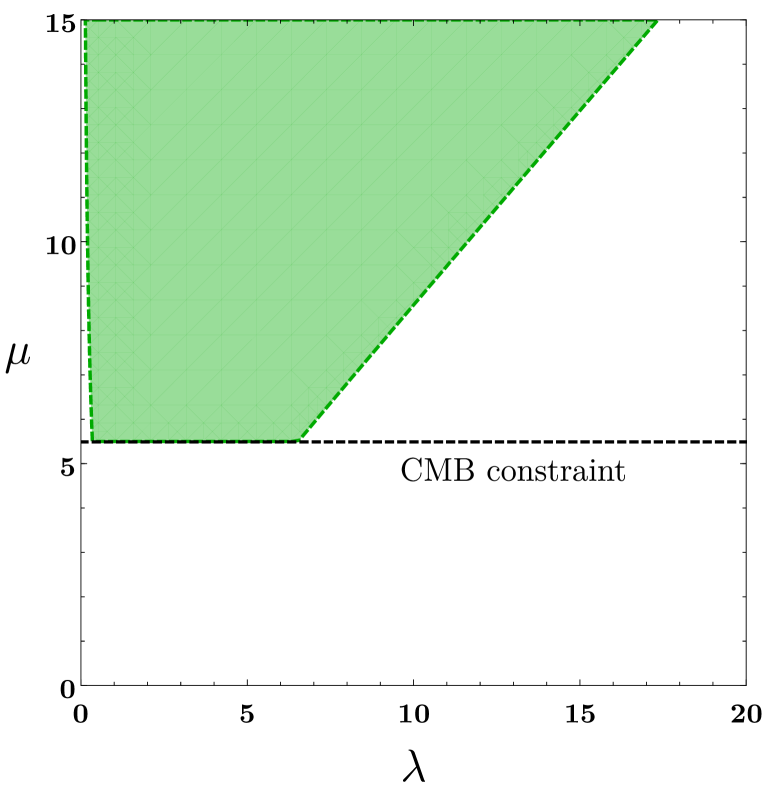
Figure 1: Parameter space in which the conditions (41) and (42) are satisfied (colored region). If the anisotropic point (b3) is responsible for the matter era, there is also the bound $\mu>5.5$ arising from the CMB constraint $\Omega_{\rm DE}<0.02$ around the redshift 50 (dashed black line). The variable $\mu$ is unbounded from above.

The point (c1) is responsible for the cosmic acceleration for $\lambda^{2}<2$. Under this condition, the point (c1) is a saddle for

$$\lambda^{2}+\lambda\mu-2>0\,,$$ (53)

whereas it is stable for $\lambda^{2}+\lambda\mu-2<0$. The condition (53) is identical to (41). This means that, as long as the anisotropic point (c2) is present, the isotropic point (c1) is a saddle. Under the condition (53), the last two eigenvalues of point (c2) in Eq. (51) are negative or complex with negative real parts. Moreover, under the condition (42) for the cosmic acceleration of point (c2), the other three eigenvalues in Eq. (51) are negative. Provided that the two inequalities (41) and (42) hold, the anisotropic dark energy dominated point (c2) is stable, while (c1) is a saddle.

In Fig. 1, we show the parameter space in the ($\lambda$, $\mu$) plane consistent with the conditions (41) and (42). We also plot the bound $\mu>5.5$ arising from the CMB constraint on point (b3). For the model parameters inside the colored region of Fig. 1, the saddle anisotropic matter point (b3) can be followed by the accelerated attractor (c2) with the non-vanishing anisotropic shear.

IV Cosmological dynamics

We study the cosmological dynamics for the coupling constants $\lambda$ and $\mu$ inside the colored region of Fig. 1. Prior to the radiation-dominated epoch, we assume the existence of an inflationary period (with subsequent reheating) driven by a scalar degree of freedom other than $\phi$. As long as such an additional scalar degree of freedom does not have specific couplings to form fields, the anisotropic shear quickly decreases during inflation. Then, the natural initial condition for the anisotropic shear at the onset of radiation era is $|\Sigma|$ very close to 0. In this case, the fixed points relevant to the early radiation era correspond to either (a1) or (a2). Indeed, we would like to show that, even if the initial condition of shear at the beginning of radiation era is close to the isotropic one ($\Sigma\simeq 0$), the solutions can approach fixed points with anisotropic hairs in the late Universe.

IV.1 Sequence of fixed points

For $\lambda>9.4$, the point (a2) can be responsible for the scaling radiation era consistent with the BBN bound. If the coupling $f(\phi)$ is absent, it is known that (a2) is followed by the isotropic matter scaling solution (b2) by reflecting the fact that the latter is stable for $\lambda^{2}>3$ CLW ; CST ; Tsuji13 . This property does not hold for the theories with $f(\phi)\neq 0$, since the point (b2) is a saddle. Instead, the point (c2) is stable for $\lambda$ and $\mu$ inside the colored region of Fig. 1. Our numerical calculations show that, for the initial conditions close to point (a2) during the radiation dominance with $\lambda>9.4$, the solutions directly approach point (c2) without passing through the scaling matter point (b2). This means the absence of a proper matter era, so the viable cosmological trajectory does not arise from the isotropic radiation scaling solution (a2).

The initial conditions in the deep radiation era realizing the viable late-time cosmology are those close to the isotropic radiation point (a1). Then, the isotropic scaling solutions (a2) and (b2) are irrelevant to the cosmological dynamics in the following discussion. We recall that the anisotropic radiation point (a3) has one less positive eigenvalues of matrix ${\cal M}$ than those of (a1). This suggests that the solutions may temporally approach point (a3) during the late radiation era. This is indeed the case for numerical analysis presented later.

The point (b1) has three negative eigenvalues of matrix ${\cal M}$, while point (b3) has two negative eigenvalues and two complex eigenvalues with negative real parts. Then, after the radiation dominance, the solutions should temporally approach the anisotropic matter point (b3) rather than the isotropic matter point (b1). As we mentioned in Sec. III.2, the point (b3) is consistent with the CMB bound $\Omega_{\rm DE}<0.02$ around the redshift $50$ for

$$\mu>5.5\,,$$ (54)

whose condition is imposed in the following. Since point (b3) is a saddle, the solutions eventually exit from the matter era driven by (b3) to reach the stable anisotropic point (c2) with cosmic acceleration.

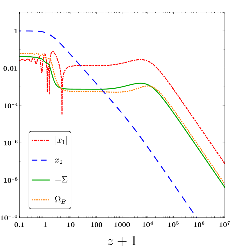
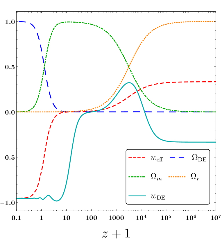
Figure 2: Evolution of $|x_{1}|$, $x_{2}$, $-\Sigma$, $\Omega_{B}$ (top) and $\Omega_{\rm DE}$, $\Omega_{r}$, $\Omega_{m}$, $w_{\rm DE}$, $w_{\rm eff}$ (bottom) versus $z+1~{}(=1/a)$ for $\lambda=2$ and $\mu=30$ with the initial conditions $x_{1}=10^{-13}$, $x_{2}=10^{-14}$, $\Sigma=0$, $\Omega_{B}=10^{-10}$, and $\Omega_{r}=0.99996$ at the redshift $z=7.9\times 10^{7}$. The present epoch (redshift $z=0$) is identified by $\Omega_{\rm DE}=0.68$.

In Fig. 2, we show the numerical solutions to $|x_{1}|$, $x_{2}$, $-\Sigma$, $\Omega_{B}$ as well as $\Omega_{\rm DE}$, $\Omega_{r}$, $\Omega_{m}$, $w_{\rm DE}$, $w_{\rm eff}$ derived by numerically integrating Eqs. (20)-(24) for $\lambda=2$ and $\mu=30$. The initial values of $x_{1}$, $x_{2}$, $\Omega_{B}$ are very much smaller than 1, so the solutions start from the regime close to the isotropic radiation point (a1). The initial condition of $\Sigma$ is chosen to be 0, but the cosmological dynamics hardly changes for $|\Sigma|$ initially much smaller than 1. The existence of non-zero $\Omega_{B}$ is crucial to generate the non-vanishing anisotropic shear at late times. As we will see below, the tiny initial value of $\Omega_{B}$ like the order $10^{-10}$ is sufficient for achieving this purpose. In Fig. 2, the condition $\Omega_{B}\gg\{x_{1}^{2},x_{2}^{2},\Sigma^{2}\}$ is satisfied in the early radiation era, so the dark energy equation of state (31) is close to $w_{\rm DE}=-1/3$ during this epoch (see the bottom panel of Fig. 2).

In Fig. 2, the radiation-dominated epoch ($\Omega_{r}\simeq 1$ and $w_{\rm eff}\simeq 1/3$) is followed by the matter-dominated era ($\Omega_{m}\simeq 1$ and $w_{\rm eff}\simeq 0$) around the redshift $z\equiv 1/a-1\simeq 3200$. The variables $|x_{1}|$, $x_{2}$, $-\Sigma$, $\Omega_{B}$ increase during the deep radiation era. After the transient period in which $w_{\rm DE}$ increases from $-1/3$ to the value close to $1/3$, the solutions enter the stage in which $|x_{1}|$, $-\Sigma$, $\Omega_{B}$ are nearly constant. The increase of $w_{\rm DE}$ continues by the radiation-matter equality. This behavior of $w_{\rm DE}$ can be interpreted as the temporal approach to the anisotropic radiation point (a3) characterized by $w_{\rm DE}=1/3$. Indeed, the numerical values of $|x_{1}|$, $\Sigma$, $\Omega_{B}$ around $z=3200$ are in fairly good agreement with their analytic values computed from Eq. (34). In other words, the anisotropic shear of order $\Sigma=-4/(3\mu^{2}+8)$ is already generated around the end of radiation era.

We note that the moment at which the transition from (a1) to (a3) takes place depends on the initial values of $x_{1}$, $x_{2}$, $\Omega_{B}$. We numerically find that there are cases in which the transition occurs much earlier compared to Fig. 2. In such cases, the solutions stay around the point (a3) characterized by $w_{\rm DE}=1/3$ for a longer period during the radiation era.

The regime in which the variables $|x_{1}|$, $-\Sigma$, $\Omega_{B}$ stay nearly constant after the radiation-matter equality corresponds to the anisotropic scaling matter fixed point (b3). From Eq. (37), we have $x_{1}=-1.36\times 10^{-2}$, $\Sigma=-7.39\times 10^{-4}$, and $\Omega_{B}=5.54\times 10^{-4}$ on point (b3), which exhibit good agreement with their numerical values around $z=60$. The dark energy density parameter on point (b3) is given by $\Omega_{\rm DE}=7.39\times 10^{-4}$, which is consistent with the CMB bound $\Omega_{\rm DE}(z=50)<0.02$. In the bottom panel of Fig. 2, we can confirm that the solutions temporally reach the region around $w_{\rm DE}=0$ during the matter era (which corresponds to the value of $w_{\rm DE}$ on point (b3)).

In the top panel of Fig. 2, we observe that $x_{2}$ exceeds $|x_{1}|$ around $z=22$. This signals the departure from the anisotropic matter fixed point (b3). Indeed, $w_{\rm DE}$ starts to deviate from 0 for $z\lesssim 30$. The anisotropic dark energy dominated point (c2) is stable for $\lambda=2$ and $\mu=30$, while the isotropic point (c1) is not. As we see in Fig. 2, the solutions finally approach the fixed point (c2) with the non-vanishing anisotropic shear after the matter-dominated epoch. From Eqs. (39) and (40), we have $x_{1}=2.76\times 10^{-2}$, $x_{2}=0.968$, $\Sigma=-4.11\times 10^{-2}$, $\Omega_{B}=6.03\times 10^{-2}$, and $w_{\rm DE}=w_{\rm eff}=-0.955$ on point (c2), which are in good agreement with their numerical values in the asymptotic future ($z\to-1$). The potential energy $V(\phi)$, which is associated with the variable $x_{2}$, is the main source for $\Omega_{\rm DE}$ at late times, but the 2-form energy density characterized by $\Omega_{B}$ also provides the non-negligible contribution to $\Omega_{\rm DE}$.

Since $x_{1}<0$ and $x_{1}>0$ on points (b3) and (c2), respectively, $x_{1}$ changes its sign during the transition from the end of matter era to the dark energy dominated epoch (around $z=3.5$ in Fig. 2). The quantity $\Sigma$, which is negative, survives during the cosmological sequence of $(\textit{a3})\to(\textit{b3})\to(\textit{c2})$. Since the 2-form energy density $\rho_{B}$ is the source for the anisotropic shear, $\Omega_{B}$ evolves in the similar way to $-\Sigma$. We note that the condition $\Sigma^{2}\ll\Omega_{B}$ is always satisfied in the numerical integration of Fig. 2, so we can ignore the terms $\Sigma^{2}$ in Eqs. (30) and (31).

In the bottom panel of Fig. 2, we find that $w_{\rm DE}$ temporally reaches the minimum value $-0.984$ around $z=3$ and then it finally approaches the asymptotic value $-0.955$ with oscillations. The quantity ${\cal F}$ in Eq. (52) is larger than 1 for $\lambda=2$ and $\mu=30$, so two of the eigenvalues of matrix ${\cal M}$ in Eq. (51) are complex with negative real parts. In this case the point (c2) is a stable spiral, so the oscillation of $w_{\rm DE}$ occurs before reaching the attractor. More generally, point (c2) is the stable spiral for ${\cal F}>1$. This condition translates to

$$4\lambda\mu^{3}+(8\lambda^{2}-11)\mu^{2}+4\lambda(\lambda^{2}+1)\mu+8(2\lambda^{2}-5)>0\,.$$ (55)

When $\lambda=1$, for example, this inequality gives $\mu>1.68$.

For the couplings satisfying $\mu\gg\lambda\geq{\cal O}(1)$, the dark energy equation of state (40) on point (c2) is approximately given by

$$w_{\rm DE}\simeq-1-\Sigma\,,$$ (56)

where

$$\Sigma\simeq-\frac{2\lambda}{3\mu}\,.$$ (57)

In the limit $\lambda/\mu\to 0$, we have $w_{\rm DE}\to-1$ with $\Sigma\to 0$. This is consistent with the no-hair theorem on the de Sitter background Wald ; Starobinsky1982mr . The coupling $f(\phi)$ in the range $0<\lambda/\mu\ll 1$ allows the possibility for realizing the late-time cosmic acceleration with the surviving anisotropic hair. If the coupling $f(\phi)$ is absent, the accelerated expansion occurs only for $\lambda<\sqrt{2}$. The numerical solution in Fig. 2 shows that $w_{\rm DE}$ close to $-1$ can be realized at low redshifts even for $\lambda>\sqrt{2}$. We also note that, for $\mu\gg\lambda\geq{\cal O}(1)$, the condition (55) is always satisfied, so the solutions finally approach the stable spiral point (c2) with the oscillation of $w_{\rm DE}$.

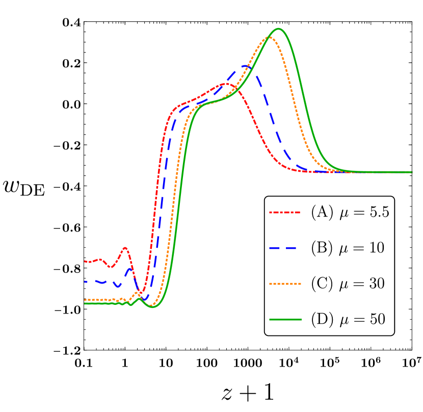
Figure 3: Evolution of $w_{\rm DE}$ versus $z+1$ for $\lambda=2$ with the same initial values of $x_{1}$, $x_{2}$, $\Sigma$, and $\Omega_{B}$, as those used in Fig. 2. Each line corresponds to (A) $\mu=5.5$, (B) $\mu=10$, (C) $\mu=30$, and (D) $\mu=50$. The initial conditions of radiation density parameter are chosen to be (A) $\Omega_{r}=0.99994$ at $z=5.5\times 10^{7}$, (B) $\Omega_{r}=0.999951$ at $z=6.5\times 10^{7}$, (C) $\Omega_{r}=0.99996$ at $z=7.9\times 10^{7}$, and (D) $\Omega_{r}=0.999961$ at $z=8.3\times 10^{7}$, respectively, to realize the value $\Omega_{r}(z=0)\simeq 10^{-4}$.

In Fig. 3, we plot the evolution of $w_{\rm DE}$ for four different values of $\mu$ by fixing $\lambda$ to be 2. As the analytic estimation (56) shows, for increasing $\mu$, the future asymptotic values of $w_{\rm DE}$ decrease toward $-1$. In case (A), i.e., $\mu=5.5$, the CMB bound $\Omega_{\rm DE}(z=50)<0.02$ is marginally satisfied, with $w_{\rm DE}=-0.70$ today. This case should be in tension with observational bounds on $w_{\rm DE}$. For larger $\mu$, however, the values of $w_{\rm DE}$ at low redshifts get smaller. In cases (B), (C), (D) of Fig. 3, today’s values of $w_{\rm DE}$ are $-0.84$, $-0.96$, and $-0.97$, respectively. Moreover, for larger $\mu$, $w_{\rm DE}$ reaches the minima closer to $-1$ at earlier cosmological epochs.

IV.2 Observational signatures

From the magnitude-redshift data of SN Ia measurements, the analysis of Ref. Campanelli:2010zx based on an anisotropic fluid showed that today’s value of $\Sigma$ is constrained to be $|\Sigma(t_{0})|\leq{\cal O}(0.01)$. For the model parameters plotted in Fig. 2, $-\Sigma(t_{0})$ is of order $0.01$. From Eq. (57), today’s value of $|\Sigma(t_{0})|$ decreases further for the smaller ratio $\lambda/\mu$, in which case the model should be well within the SN Ia bound.

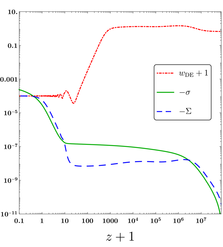
Figure 4: Evolution of $-\sigma$, $-\Sigma$, and $w_{\rm DE}+1$ versus $z+1$ for $\lambda=1.5$ and $\mu=10^{4}$. The initial conditions are chosen to be $x_{1}=10^{-13}$, $x_{2}=10^{-14}$, $\Sigma=0$, $\Omega_{B}=10^{-10}$, $\Omega_{r}=0.999965$, and $\sigma=0$ at the redshift $z=9.1\times 10^{7}$.

The time variation of $\sigma$ after decoupling also leads to the modification to CMB temperature anisotropies Koivisto:2007bp ; Koivisto:2008ig . The spatial metric tensor $g_{ij}$ for the line element (3) is expressed in the form $g_{ij}=a^{2}(t)\gamma_{ij}$, where $\gamma_{ij}$ is the anisotropic contribution containing $\sigma(t)$. Defining $\sigma_{ij}\equiv\dot{\gamma}_{ij}/2$, the CMB temperature anisotropy due to the anisotropic shear is quantified as Appleby:2009za

$$\frac{\delta T}{T}(\hat{n})=-\int_{t_{\rm de}}^{t_{0}}\sigma_{ij}\hat{n}^{i}\hat{n}^{j}\rm{d}t\,,$$ (58)

where $t_{\rm de}$ and $t_{0}$ correspond to the cosmic time at decoupling ($z\simeq 1090$) and today ($z=0$), respectively, and $\hat{n}$ is the line-of-sight unit vector. The scalar product $\sigma_{ij}\hat{n}^{i}\hat{n}^{j}$ is at most of order $\dot{\sigma}$ and hence

$$\left|\frac{\delta T}{T}(\hat{n})\right|\lesssim\left|\int_{t_{\rm de}}^{t_{0}}\dot{\sigma}\,\rm{d}t\right|=\left|\sigma(t_{0})-\sigma(t_{\rm de})\right|\,.$$ (59)

Provided that the right hand side of Eq. (59) is much smaller than 1, the anisotropic shear mostly affects the CMB quadrupole. According to the analysis of Ref. Appleby:2009za , the conservative criterion for the consistency with the CMB quadrupole data should be around $\left|\sigma(t_{0})-\sigma(t_{\rm de})\right|<10^{-4}$.

Since $\sigma^{\prime}=\Sigma$, the quantity $\left|\sigma(t_{0})-\sigma(t_{\rm de})\right|$ is related to the asymptotic value $\Sigma\simeq-2\lambda/(3\mu)$ on point (c2) and the other value $\Sigma=-2/(3\mu^{2}+8)$ on point (b3). In Fig. 4, we plot the evolution of $-\sigma$ and $-\Sigma$ for $\lambda=1.5$ and $\mu=10^{4}$ by choosing their initial conditions to be 0. As estimated analytically, $-\Sigma$ temporally reaches the nearly constant value $6.7\times 10^{-9}$ in the matter era and finally approaches the asymptotic value $1.0\times 10^{-4}$. In this case, the numerical values of $-\sigma$ today and at decoupling are given, respectively, by $-\sigma(t_{0})=2.8\times 10^{-5}$ and $-\sigma(t_{\rm de})=1.2\times 10^{-7}$, so that $\left|\sigma(t_{0})-\sigma(t_{\rm de})\right|=2.8\times 10^{-5}<10^{-4}$.

The above discussion shows that the models in which both $\mu/\lambda$ and $\mu$ are much larger than the order 1 can be consistent with the CMB quadrupole bound. For such model parameters, the deviation of $w_{\rm DE}$ from $-1$ is small on the attractor point (c2), see Eq. (56) with Eq. (57). In Fig. 4, we observe that $w_{\rm DE}$ approaches the value around $-1$ at high redshifts. The evolution of $w_{\rm DE}$ close to $-1$ at low redshifts is realized by the coupling between 2-form and scalar fields even for the scalar exponential potential with $\lambda>\sqrt{2}$. Moreover, our anisotropic dark energy model with $\left|\sigma(t_{0})-\sigma(t_{\rm de})\right|={\cal O}(10^{-5})$ can leave interesting signatures in the CMB quadrupole anisotropy, which may be used to alleviate the observed quadrupole anomaly problem Aghanim:2018eyx .

V Conclusions

We proposed a novel anisotropic dark energy model in which a quintessence scalar $\phi$ is coupled to a 2-form field strength $H_{\alpha\beta\gamma}$ with the interacting Lagrangian $-f(\phi)H_{\alpha\beta\gamma}H^{\alpha\beta\gamma}/12$. For the exponential scalar potential $V(\phi)=V_{0}e^{-\lambda\phi/M_{\rm pl}}$ with the coupling $f(\phi)=f_{0}e^{-\mu\phi/M_{\rm pl}}$, we showed that the late-time cosmic acceleration with the dark energy equation of state $w_{\rm DE}$ close to $-1$ can be realized even for $\lambda\geq{\cal O}(1)$. This property comes from the fact that there exists the anisotropic accelerated attractor fixed point (c2) supported by the 2-form density parameter $\Omega_{B}$ and the shear $\Sigma$.

Even for initial conditions close to the isotropic radiation point (a1), we showed that the solutions temporally reach the saddle anisotropic point (a3) by the end of the radiation era and then they are followed by the saddle anisotropic matter scaling solution (b3) with constant $\Sigma$ and $\Omega_{B}$. From the CMB bound $\Omega_{\rm DE}(z=50)<0.02$ on the scaling matter fixed point (b3), the coupling constant $\mu$ is constrained to be $\mu>5.5$. Provided that the two conditions (41) and (42) are satisfied, the fixed point (c2) corresponds to the accelerated attractor with non-vanishing anisotropic hair.

In summary, the typical cosmological evolution is given by the trajectory,

$$(\textit{a1})\to(\textit{a3})\to(\textit{b3})\to(\textit{c2})\,.$$ (60)

For the couplings in the range $\mu\gg\lambda\geq{\cal O}(1)$, we numerically confirmed the above cosmological sequence, see e.g., Fig. 2. The analytic derivation of point (c2) showed that, for the larger ratio $\mu/\lambda$, the future asymptotic values of $w_{\rm DE}$ tend to be smaller, which is the case for the numerical integration in Fig. 3. Before reaching the attractor, $w_{\rm DE}$ exhibits oscillations in the range $w_{\rm DE}>-1$. This property can be used to distinguish our model from quintessence and the $\Lambda$CDM model.

The existence of non-vanishing anisotropic shear after the radiation-dominated epoch leaves imprints on observables associated with CMB and SN Ia measurements. In particular, the time variation of spatial shear $\sigma$ after decoupling to today affects the CMB quadrupole temperature anisotropy. When both $\mu/\lambda$ and $\mu$ are much larger than unity, we showed that the change of spatial shear from decoupling to today can be compatible with the CMB quadrupole data. In particular, if $\left|\sigma(t_{0})-\sigma(t_{\rm de})\right|$ is of order $10^{-5}$, there may be an interesting possibility for addressing the problem of CMB quadrupole anomaly. We leave detailed observational constraints on the parameters $\mu$ and $\lambda$ for a future work.

Appendix A Other fixed points

In this Appendix, we present two additional fixed points (a4) and (b4), which are irrelevant to the radiation, matter, dark energy dominated epochs.

$\bullet$ (a4) Anisotropic scaling solution with $w_{\rm eff}=1/3$

$$x_{1}=\frac{2\sqrt{6}}{3\lambda}\,,\quad x_{2}=\frac{\sqrt{3(6\mu^{2}+3\lambda\mu+16)}}{6\lambda}\,,$$

$$\Sigma=-\frac{\lambda+2\mu}{2\lambda}\,,\quad\Omega_{B}=\frac{\lambda+2\mu}{4\lambda}\,,$$

$$\Omega_{r}=\frac{2\lambda^{2}-7\lambda\mu-6\mu^{2}-16}{4\lambda^{2}}\,,\quad\Omega_{m}=0\,,$$ (61)

with $\Omega_{\rm DE}=(2\lambda^{2}+7\lambda\mu+6\mu^{2}+16)/(4\lambda^{2})$ and $w_{\rm DE}=1/3$. In the limit $\mu\to-\lambda/2$, this point reduces to the isotropic radiation scaling solution (a2). Since $w_{\rm eff}=1/3$ on point (a4), it can be used only for the radiation era. For $\lambda$ and $\mu$ in the range (15), however, $\Omega_{r}$ can not be close to 1.

$\bullet$ (b4) Anisotropic scaling solution with $w_{\rm eff}=0$

$$x_{1}=\frac{\sqrt{6}}{2\lambda}\,,\quad x_{2}=\frac{\sqrt{3(3\mu^{2}+\lambda\mu+8)}}{4\lambda}\,,$$

$$\Sigma=-\frac{\lambda+3\mu}{4\lambda}\,,\quad\Omega_{B}=\frac{3(\lambda+3\mu)}{16\lambda}\,,$$

$$\Omega_{r}=0\,,\quad\Omega_{m}=\frac{3(2\lambda^{2}-3\lambda\mu-3\mu^{2}-8)}{8\lambda^{2}}\,,$$ (62)

with $\Omega_{\rm DE}=(2\lambda^{2}+9\lambda\mu+9\mu^{2}+24)/(8\lambda^{2})$ and $w_{\rm DE}=0$. In the limit $\mu\to-\lambda/3$, this recovers the isotropic matter scaling solution (b2). Since $w_{\rm eff}=0$ on point (b4), it is relevant only to the matter era. For $\lambda$ and $\mu$ in the range (15), however, $\Omega_{m}$ is away from 1.

References

- (1) A. G. Riess et al., Astron. J. 116, 1009 (1998) [astro-ph/9805201].
- (2) S. Perlmutter et al., Astrophys. J. 517, 565 (1999) [astro-ph/9812133].
- (3) S. Weinberg, Rev. Mod. Phys. 61, 1 (1989).
- (4) Y. Fujii, Phys. Rev. D 26, 2580 (1982).
- (5) L. H. Ford, Phys. Rev. D 35, 2339 (1987).
- (6) B. Ratra and P. J. E. Peebles, Phys. Rev. D 37, 3406 (1988).
- (7) C. Wetterich, Nucl. Phys. B 302, 668 (1988) [arXiv:1711.03844 [hep-th]].
- (8) T. Chiba, N. Sugiyama and T. Nakamura, Mon. Not. Roy. Astron. Soc. 289, L5 (1997) [astro-ph/9704199].
- (9) P. G. Ferreira and M. Joyce, Phys. Rev. Lett. 79, 4740 (1997) [astro-ph/9707286].
- (10) R. R. Caldwell, R. Dave and P. J. Steinhardt, Phys. Rev. Lett. 80, 1582 (1998) [astro-ph/9708069].
- (11) E. J. Copeland, A. R. Liddle and D. Wands, Phys. Rev. D 57, 4686 (1998) [gr-qc/9711068].
- (12) E. J. Copeland, M. Sami and S. Tsujikawa, Int. J. Mod. Phys. D 15, 1753 (2006) [hep-th/0603057].
- (13) S. Tsujikawa, Class. Quant. Grav. 30, 214003 (2013) [arXiv:1304.1961 [gr-qc]].
- (14) J. Garriga and A. Vilenkin, Phys. Rev. D 64, 023517 (2001) [hep-th/0011262].
- (15) R. Emparan and J. Garriga, JHEP 0305, 028 (2003) [hep-th/0304124].
- (16) P. K. Townsend and M. N. R. Wohlfarth, Phys. Rev. Lett. 91, 061302 (2003) [hep-th/0303097].
- (17) N. Ohta, Phys. Rev. Lett. 91, 061303 (2003) [hep-th/0303238].
- (18) M. N. R. Wohlfarth, Phys. Lett. B 563, 1 (2003) [hep-th/0304089].
- (19) S. Roy, Phys. Lett. B 567, 322 (2003) [hep-th/0304084].
- (20) G. Obied, H. Ooguri, L. Spodyneiko and C. Vafa, arXiv:1806.08362 [hep-th].
- (21) P. Agrawal, G. Obied, P. J. Steinhardt and C. Vafa, Phys. Lett. B 784, 271 (2018) [arXiv:1806.09718 [hep-th]].
- (22) M. B. Green, J. H. Schwarz, and E. Witten, “Superstring theory”, Cambridge University Press, Cambridge (1987).
- (23) J. P. Beltrán Almeida, A. Guarnizo and C. A. Valenzuela-Toledo, arXiv:1810.05301 [astro-ph.CO].
- (24) B. Ratra, Astrophys. J. 391, L1 (1992).
- (25) K. Bamba and J. Yokoyama, Phys. Rev. D 69, 043507 (2004) [astro-ph/0310824].
- (26) J. Martin and J. Yokoyama, JCAP 0801, 025 (2008) [arXiv:0711.4307 [astro-ph]].
- (27) S. Yokoyama and J. Soda, JCAP 0808, 005 (2008) [arXiv:0805.4265 [astro-ph]].
- (28) K. Dimopoulos, M. Karciauskas and J. M. Wagstaff, Phys. Rev. D 81, 023522 (2010) [arXiv:0907.1838 [hep-ph]].
- (29) K. Dimopoulos, M. Karciauskas and J. M. Wagstaff, Phys. Lett. B 683, 298 (2010) [arXiv:0909.0475 [hep-ph]].
- (30) T. Fujita, I. Obata, T. Tanaka and S. Yokoyama, JCAP 1807, 023 (2018) [arXiv:1801.02778 [astro-ph.CO]].
- (31) M. a. Watanabe, S. Kanno and J. Soda, Phys. Rev. Lett. 102, 191302 (2009) [arXiv:0902.2833 [hep-th]].
- (32) M. a. Watanabe, S. Kanno and J. Soda, Mon. Not. Roy. Astron. Soc. 412, L83 (2011) [arXiv:1011.3604 [astro-ph.CO]].
- (33) S. Kanno, J. Soda and M. a. Watanabe, JCAP 1012, 024 (2010) [arXiv:1010.5307 [hep-th]].
- (34) J. Ohashi, J. Soda and S. Tsujikawa, Phys. Rev. D 88, 103517 (2013) [arXiv:1310.3053 [hep-th]].
- (35) A. E. Gumrukcuoglu, B. Himmetoglu and M. Peloso, Phys. Rev. D 81, 063528 (2010) [arXiv:1001.4088 [astro-ph.CO]].
- (36) A. E. Gumrukcuoglu, C. R. Contaldi and M. Peloso, JCAP 0711, 005 (2007) [arXiv:0707.4179 [astro-ph]].
- (37) B. Himmetoglu, JCAP 1003, 023 (2010) [arXiv:0910.3235 [astro-ph.CO]].
- (38) N. Bartolo, S. Matarrese, M. Peloso and A. Ricciardone, Phys. Rev. D 87, 023504 (2013) [arXiv:1210.3257 [astro-ph.CO]].
- (39) R. Namba, Phys. Rev. D 86, 083518 (2012) [arXiv:1207.5547 [astro-ph.CO]].
- (40) M. Shiraishi, E. Komatsu, M. Peloso and N. Barnaby, JCAP 1305, 002 (2013) [arXiv:1302.3056 [astro-ph.CO]].
- (41) T. Fujita and S. Yokoyama, JCAP 1309, 009 (2013) [arXiv:1306.2992 [astro-ph.CO]].
- (42) J. Ohashi, J. Soda and S. Tsujikawa, Phys. Rev. D 87, 083520 (2013) [arXiv:1303.7340 [astro-ph.CO]].
- (43) A. Ito and J. Soda, Phys. Rev. D 92, 123533 (2015) [arXiv:1506.02450 [hep-th]].
- (44) I. Obata and T. Fujita, Phys. Rev. D 99, 023513 (2019) [arXiv:1808.00548 [astro-ph.CO]].
- (45) J. P. B. Almeida, A. Guarnizo, R. Kase, S. Tsujikawa and C. A. Valenzuela-Toledo, arXiv:1901.06097 [gr-qc].
- (46) J. Ohashi, J. Soda and S. Tsujikawa, JCAP 1312, 009 (2013) [arXiv:1308.4488 [astro-ph.CO]].
- (47) M. Thorsrud, D. F. Mota and S. Hervik, JHEP 1210, 066 (2012) [arXiv:1205.6261 [hep-th]].
- (48) T. Koivisto and D. F. Mota, Astrophys. J. 679, 1 (2008) [arXiv:0707.0279 [astro-ph]].
- (49) T. Koivisto and D. F. Mota, JCAP 0806, 018 (2008) [arXiv:0801.3676 [astro-ph]].
- (50) R. Battye and A. Moss, Phys. Rev. D 80, 023531 (2009) [arXiv:0905.3403 [astro-ph.CO]].
- (51) S. Appleby, R. Battye and A. Moss, Phys. Rev. D 81, 081301 (2010) [arXiv:0912.0397 [astro-ph.CO]].
- (52) L. Campanelli, P. Cea, G. L. Fogli and A. Marrone, Phys. Rev. D 83, 103503 (2011) [arXiv:1012.5596 [astro-ph.CO]].
- (53) S. A. Appleby and E. V. Linder, Phys. Rev. D 87, 023532 (2013) [arXiv:1210.8221 [astro-ph.CO]].
- (54) M. Betoule et al. [SDSS Collaboration], Astron. Astrophys. 568, A22 (2014) [arXiv:1401.4064 [astro-ph.CO]].
- (55) N. Aghanim et al. [Planck Collaboration], arXiv:1807.06209 [astro-ph.CO].
- (56) D. Giannakis and W. Hu, Phys. Rev. D 72, 063502 (2005) [astro-ph/0501423].
- (57) F. Arroja and M. Sasaki, Phys. Rev. D 81, 107301 (2010) [arXiv:1002.1376 [astro-ph.CO]].
- (58) R. Kase and S. Tsujikawa, Phys. Rev. D 90, 044073 (2014) [arXiv:1407.0794 [hep-th]].
- (59) R. Bean, S. H. Hansen and A. Melchiorri, Phys. Rev. D 64, 103508 (2001) [astro-ph/0104162].
- (60) J. Ohashi and S. Tsujikawa, Phys. Rev. D 80, 103513 (2009) [arXiv:0909.3924 [gr-qc]].
- (61) P. A. R. Ade et al. [Planck Collaboration], Astron. Astrophys. 594, A14 (2016) [arXiv:1502.01590 [astro-ph.CO]].
- (62) R. M. Wald, Phys. Rev. D 28, 2118 (1983).
- (63) A. A. Starobinsky, JETP Lett. 37, 66 (1983).