Magnetization and entanglement after a geometric quench in the XXZ chain

Abstract

We investigate the dynamics of the XXZ spin chain after a geometric quench, which is realized by connecting two half-chains prepared in their ground states with zero and maximum magnetizations, respectively. The profiles of magnetization after the subsequent time evolution are studied numerically by density-matrix renormalization group methods, and a comparison to the predictions of generalized hydrodynamics yields a very good agreement. We also calculate the profiles of entanglement entropy and propose an ansatz for the noninteracting XX case, based on arguments from conformal field theory. In the general interacting case, the propagation of the entropy front is studied numerically both before and after the reflection from the chain boundaries. Finally, our results for the magnetization fluctuations indicate a leading order proportionality relation to the entanglement entropy.

I Introduction

The dynamics of closed many-body quantum systems has been the topic of a vast amount of research activities Polkovnikov et al. (2011); Gogolin and Eisert (2016), with a special attention devoted to integrable models Calabrese et al. (2016). The most commonly studied scenarios include the quantum quench Essler and Fagotti (2016) and the subsequent relaxation towards a stationary state Vidmar and Rigol (2016). A special feature of integrable systems is that, due to the existence of stable quasiparticle excitations, a nonequilibrium steady state supporting persistent currents may emerge. The transport properties in systems driven by initial inhomogeneities have been the subject of numerous investigations, see the review Vasseur and Moore (2016) and references therein.

An important breakthrough in the understanding of transport has been the development of a hydrodynamic theory Bertini et al. (2016); Castro-Alvaredo et al. (2016), which could properly account for the nontrivial conservation laws of interacting integrable systems. Originally formulated for partitioned initial states Bertini et al. (2016); Castro-Alvaredo et al. (2016); Piroli et al. (2017), the theory of generalized hydrodynamics (GHD) has since been extended to include slowly varying inhomogeneities Doyon and Yoshimura (2017); Doyon et al. (2017a, b); Caux et al. ; Bulchandani et al. (2017, 2018) and applied to a variety of integrable models Ilievski and De Nardis (2017); Doyon et al. (2018); Mazza et al. (2018); Mestyán et al. (2019). Although GHD implies in general a ballistic transport, recently it has been shown how diffusive mechanisms, observed numerically in particular cases Misguich et al. (2017); Ljubotina et al. (2017); Stéphan (2017); Collura et al. (2018), can be incorporated into the theory De Nardis et al. (2018)

The GHD formalism has proved to be very successful in describing the time evolution of magnetization or density profiles starting from an inhomogeneous inital state. Another very important question is, however, how entanglement spreads out in the time-evolved state. After a global quench in a homogeneous interacting system, this can be answered by ascribing the growth of entropy to entangled pairs of quasiparticles Calabrese and Cardy (2005), and finding the corresponding entropy production rates Alba and Calabrese (2017, 2018). Furthermore, since the description is based on quasiparticles, there have been attempts to use the machinery of GHD to understand entanglement evolution from inhomogeneous initial states Alba (2018); Bertini et al. (2018).

The quasiparticle interpretation yields, by construction, a linear growth of entanglement in time. In contrast, in a number of inhomogeneous situations such as front evolution from domain walls or initial states created by slowly varying potentials Gobert et al. (2005); Eisler et al. (2009); Sabetta and Misguich (2013); Eisler and Peschel (2014); Dubail et al. (2017a, b); Eisler and Bauernfeind (2017); Eisler et al. (2016); Eisler and Maislinger (2018), it has been observed that the growth of entanglement is much slower, at most logarithmic. In the quasiparticle picture, these correspond to zero entropy density states, and the hydrodynamic information alone is not sufficient to account for the growth of entanglement. For the particular case of the domain-wall quench, further insight is provided by a special conformal field theory (CFT) treatment Dubail et al. (2017a) which is, however, restricted to noninteracting fermions. Hence the general mechanism leading to a sublinear growth of entanglement still remains elusive.

In this paper we will study such a problem by considering the so-called geometric quench Mossel et al. (2010); Alba and Heidrich-Meisner (2014) in the XXZ spin chain or, equivalently, fermions with nearest-neighbor interactions. The quench protocol simply consists of releasing the ground state of a chain, by joining it to another one prepared in the vacuum. We show that the magnetization profiles can be perfectly reproduced using the GHD formalism and we find that they depend qualitatively on the sign of the interaction, as opposed to the simpler setup of a domain-wall initial state Collura et al. (2018). Furthermore, with the help of some heuristic CFT arguments, we put forward an ansatz for the entanglement profile in the noninteracting case, which gives a very good description of the numerical data. Although the generalization to the interacting case does not seem to be straightforward, our numerical results show a qualitatively similar behavior of the entropy profiles, with expansion velocities that are obtained from the GHD solution of the dynamics. Finally, by studying the fluctuations of the subsystem magnetization, we observe that they are approximately proportional to the entropy within the entire front region, which seems to hold for a large range of interactions.

The rest of the manuscript is structured as follows. In Section II we introduce our setup and give a brief overview of the model. In Sec. III we present the magnetization profiles, starting with a review of GHD and followed by our numerical results, whereas the entropy profiles are discussed in Sec. IV. Reflections due to boundaries are studied in Sec. V and a comparison between magnetization fluctuations and entropy can be found in Sec. VI. Our closing remarks are given in Sec. VII followed by an Appendix containing details of the calculation for the edge profile.

II Model and setup

We consider the XXZ spin chain which is given by the Hamiltonian

$$H=J\sum_{j=1}^{L-1}\left(S^{x}_{j}S^{x}_{j+1}+S^{y}_{j}S^{y}_{j+1}+\Delta S^{z}_{j}S^{z}_{j+1}\right)$$ (1)

where $S^{\alpha}_{j}$ are spin-1/2 operators acting on site $j$, $J$ is the coupling and $\Delta$ the anisotropy parameter. We set $J=1$ and consider open boundary conditions on a chain of length $L$. The XXZ model is equivalent to a chain of spinless fermions with nearest-neighbor interactions of strength $\Delta$, with $\Delta=0$ corresponding to the free-fermion point.

The protocol of the geometric quench is illustrated in Fig. 1. Initially, the chain is split in two halves and the left hand side is initialized in the ground state $\ket{GS}$ of an XXZ chain of length $L/2$. On the other hand, the right half-chain is prepared in the fully polarized state $\ket{\downarrow\downarrow\downarrow\dots}$, or the vacuum state in the fermionic language. Subsequently, the two half-chains are joined together at $t=0$ and the system is let evolve unitarily

$$\ket{\psi(t)}=\mathrm{e}^{-iHt}\ket{GS}\otimes\ket{\downarrow\downarrow\downarrow\dots}$$ (2)

governed by the Hamiltonian in Eq. (1). In other words, we would like to study how the ground state prepared on a half-chain expands into vacuum after an instantaneous change of geometry (i.e. the size of the chain), hence the term geometric quench. We are primarily interested in the magnetization $\braket{S^{z}_{j}}\equiv\bra{\psi(t)}S^{z}_{j}\ket{\psi(t)}$ and the entanglement profile, as measured by the entanglement entropy between two segments $A$ and $B$, as depicted in Fig. 1.

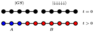
Figure 1: Setup of the geometric quench.

The ground state of the XXZ chain can be constructed with the help of Bethe Ansatz Takahashi (1999); Franchini (2017). Here we will focus on the regime $|\Delta|<1$ where the ground state is a gapless Luttinger liquid Giamarchi (2003), and we use the standard parametrization $\Delta=\cos(\gamma)$. The quasiparticle excitations of the XXZ chain are created upon the vacuum state $\ket{\downarrow\downarrow\downarrow\dots}$ and are labelled by their rapidity $\lambda$. They satisfy appropriate quantization conditions, as given by the roots of the Bethe equations. In particular, the ground state involves only magnons with real $\lambda$, but in general the solutions admit a family of string excitations Takahashi (1999), corresponding to roots parallel to the imaginary axis. In the thermodynamic limit $L\to\infty$, and in the zero-magnetization sector, the roots on the real axis become continuous and their density $\rho(\lambda)$ satisfies the linear integral equation

$$\rho(\lambda)+\int_{-\infty}^{\infty}\frac{\differential\mu}{2\pi}\mathcal{K}(\lambda-\mu)\rho(\mu)=\frac{p^{\prime}(\lambda)}{2\pi}.$$ (3)

Note that the r.h.s. of Eq. (3) contains the derivative of the bare momentum $p^{\prime}(\lambda)=\theta^{\prime}_{1}(\lambda)$, while the integral on the left is due to elastic scattering between quasiparticles, with the kernel $\mathcal{K}(\lambda)=\theta^{\prime}_{2}(\lambda)$ being the differential scattering phase. Both of them are given via

$$\theta^{\prime}_{n}(\lambda)=\frac{\sin(n\gamma)}{\cosh(\lambda)-\cos(n\gamma)},\qquad n=1,2\,.$$ (4)

In fact, Eq. (3) is just a simple example of the so-called dressing operation, where a certain function of the rapidity gets modified by the presence of the other quasiparticles. The dressed version $f^{dr}$ of a bare function $f$ is defined as the solution of

$$f^{dr}(\lambda)+\int_{-\infty}^{\infty}\frac{\differential\mu}{2\pi}\mathcal{K}(\lambda-\mu)n(\mu)f^{dr}(\mu)=f(\lambda)\,,$$ (5)

which is a Fredholm-type integral equation and can be solved numerically Atkinson and Shampine (2008). Here, $n(\mu)$ is the occupation function, i.e. the ratio of the particle density (occupied rapidities) and the total root density, including the density of holes (unoccupied rapidities). However, since the XXZ ground state does not contain holes, one has $n(\mu)\equiv 1$. Hence, the root density is just proportional to the derivative of the dressed momentum, $2\pi\rho(\lambda)=p^{\prime dr}(\lambda)$. Another important quantity we shall need is the dressed quasiparticle energy $e^{dr}(\lambda)$, which follows from (5) with the bare energy given by

$$e(\lambda)=\frac{-\sin^{2}(\gamma)}{\cosh(\lambda)-\cos(\gamma)}\,.$$ (6)

On the numerical side, we carry out density-matrix renormalization group (DMRG) calculations Schollwöck (2011), using the ITensor C++ library ite . The ground-state search is performed by applying DMRG on the left half-chain, whereas the vacuum state on the right half-chain has a trivial matrix product state representation. After the quench, the time evolution is done by applying tDMRG with a timestep of $\delta t=0.05$, a truncated weight of $10^{-10}$ and a maximum bond dimension of $\chi_{max}=1200$.

III Magnetization Profiles

We start our study of the geometric quench with a discussion of the magnetization profiles. Before presenting our numerical results, we shall introduce an efficient method that has been developed recently for the study of transport in integrable systems.

III.1 Generalized hydrodynamics

The understanding of time evolution in integrable models due to initial inhomogeneities has recently come to a breakthrough by the development of generalized hydrodynamics Bertini et al. (2016); Castro-Alvaredo et al. (2016). The idea of GHD is to give an effective description of the dynamics and the underlying state at a hydrodynamic scale. Indeed, in interacting integrable models the quasiparticle excitations are moving freely, experiencing only phase shifts due to the scattering on other quasiparticles. One then assumes that, for large times $t$ and large distances $x$ from the inhomogeneity, a dynamical equilibrium emerges, and the system is described by a local quasi-stationary state (LQSS).

For the class of initial states, where the inhomogeneity is solely due to the junction of two, otherwise homogeneous states without any inherent length scale, the LQSS depends only on the ray variable $\zeta=\frac{x}{t}$. Assuming that there is only one type of quasiparticles involved (such as for the geometric quench), specifying the LQSS amounts to finding the particle density $\rho_{\zeta}(\lambda)$ that varies along the rays. The kinetic theory of quasiparticles eventually leads to the continuity equation Bertini et al. (2016); Castro-Alvaredo et al. (2016)

$$\partial_{t}\rho_{\zeta}(\lambda)+\partial_{x}(v(\lambda)\rho_{\zeta}(\lambda))=0\,,$$ (7)

where the velocity $v(\lambda)$ is given by the dressed quasiparticle group velocity

$$v(\lambda)=\frac{e^{\prime dr}(\lambda)}{p^{\prime dr}(\lambda)}.$$ (8)

The GHD equation (7) could be interpreted as an infinite set of continuity equations for each $\lambda$, corresponding to the infinite set of conserved charges that are present for integrable models. Despite its apparent simplicity, one should stress that the solution of (7) is, in general, nontrivial since the dressed velocity (8) itself depends on the quasiparticle density. Indeed, the dressing operation (5) contains information about the full occupation function $n_{\zeta}(\lambda)$, and thus Eq. (7) has to be solved self-consistently. However, if the densities depend only on the ray variable $\zeta$, the GHD equation could be shown to simplify to Bertini et al. (2016); Castro-Alvaredo et al. (2016)

$$(\zeta-v(\lambda))\,\partial_{\zeta}n_{\zeta}(\lambda)=0\,,$$ (9)

which has the piecewise continuous solution

$$n_{\zeta}(\lambda)=\Theta(v(\lambda)-\zeta)n_{L}(\lambda)+\Theta(\zeta-v(\lambda))n_{R}(\lambda)\,,$$ (10)

where $\Theta$ is the Heaviside step function and $n_{L/R}(\lambda)$ is the initial occupation on the left/right half-chain.

The solution (10) has a clear physical interpretation, namely that the information on the initial occupations gets transported by the quasiparticles. Along a given ray $\zeta>0$ in the r.h.s. of the chain, only the quasiparticles emitted from the left half-chain become visible that have sufficient velocity $v(\lambda)>\zeta$ to arrive there. Similarly, for $\zeta<0$ the quasiparticles are emitted from the right half-chain and propagate to the left. Thus, for the simple initial states considered here, solving the GHD equation boils down to determining the solution to $v(\lambda)=\zeta$, where the dressing of the velocity is calculated with respect to the occupation function in (10).

The situation further simplifies for the geometric quench, since the ground-state occupation is given by $n_{L}(\lambda)=1$, whereas for the vacuum one trivially has $n_{R}(\lambda)=0$. We shall first assume, that the dressed velocity is a monotonically increasing function with a unique solution $v(\lambda_{*})=\zeta$ for each $\zeta$ and hence

$$n_{\zeta}(\lambda)=\Theta(\lambda-\lambda_{*})\,.$$ (11)

One has thus the condition that the function

$$v(\lambda_{*})=\frac{e^{\prime dr}(\lambda_{*})}{p^{\prime dr}(\lambda_{*})}$$ (12)

has to be monotonously increasing, when the dressing is evaluated with the occupation in (11), i.e. the integrals in (5) are carried out over $\left[\lambda_{*},\infty\right)$. The velocity (12) can be evaluated numerically and the result is shown in Fig. 2 for various $\Delta$. One can see clearly, that our assumption is satisfied only for attractive interactions $\Delta<0$, whereas for the repulsive case $\Delta>0$ the velocity $v(\lambda_{*})$ develops a maximum.

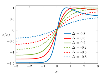
Figure 2: Dressed velocity $v(\lambda_{*})$ corresponding to the occupation function in Eq. (11), for several values of $\Delta$.

The above discrepancy can be understood as follows. For $\Delta<0$, the maximum velocity occurs for $\lambda_{*}\to\infty$, which gives the expansion velocity of the front into vacuum. Note that in this limit the occupation (11) vanishes completely, and thus the group velocity is given by its bare (undressed) value

$$v_{0}(\lambda)=\frac{e^{\prime}(\lambda)}{p^{\prime}(\lambda)}=\frac{\sin(\gamma)\sinh(\lambda)}{\cosh(\lambda)-\cos(\gamma)}\,.$$ (13)

In particular, one has

$$v_{0}(\lambda\to\infty)=\sin(\gamma)\,,$$ (14)

which turns out to be the real maximum for $\Delta<0$. However, for $\Delta>0$, the equation $v^{\prime}_{0}(\tilde{\lambda})=0$ has a nontrivial solution with

$$\cosh\small(\tilde{\lambda}\small)=\frac{1}{\Delta}\,.$$ (15)

The maximum velocity thus occurs at a finite value of the rapidity, and one obtains $v_{0}(\tilde{\lambda})=1$, independently of $\Delta$. Consequently, the ansatz for the occupation function has to be modified as

$$n_{\zeta}(\lambda)=\Theta(\lambda-\lambda_{1})\Theta(\lambda_{2}-\lambda)\,,$$ (16)

where the velocities must satisfy

$$v(\lambda_{1})=v(\lambda_{2})=\zeta\,.$$ (17)

Note that the rapidities $\lambda_{1}<\tilde{\lambda}<\lambda_{2}$ are located on different sides of the maximum and can be found iteratively.

Interestingly, the GHD solution for the geometric quench yields different vacuum expansion velocities, with the rightmost ray given by $\zeta_{max}=1$ and $\zeta_{max}=\sin(\gamma)$ for positive and negative values of $\Delta$, respectively. Note, however, that by decreasing $\zeta$, the solution $\lambda_{2}$ of (17) eventually goes to infinity, and thus the ansatz (16) actually goes over to (11) with $\lambda_{1}\to\lambda_{*}$. In particular, one finds that the minimum of the dressed velocity occurs for $\lambda_{*}\to-\infty$ (see Fig. 2), where (11) simply corresponds to the ground-state occupation. Therefore, the leftmost ray is given via the spinon velocity Franchini (2017)

$$\zeta_{min}=-v_{s}=-\frac{\pi}{2}\frac{\sin(\gamma)}{\gamma}\,.$$ (18)

Finally, in order to obtain the magnetization profile, one needs the particle density $\rho_{\zeta}(\lambda)$. This is given explicitly by

$$\rho_{\zeta}(\lambda)=n_{\zeta}(\lambda)\frac{p^{\prime dr}(\lambda)}{2\pi}\,,$$ (19)

where the dressing is calculated with an occupation $n_{\zeta}(\lambda)$ that corresponds to either (11) or (16). In turn, the magnetization is given by

$$\expectationvalue{S^{z}}=-\frac{1}{2}+\int\rho_{\zeta}(\lambda)d\lambda\,.$$ (20)

Although in general the GHD ansatz requires a numerical solution of the integral equations for the dressing, there is one particular regime where an approximate analytical result can be given. Namely, for $\Delta>0$ the magnetization profile around the $\zeta_{max}=1$ edge can be obtained to leading order via a perturbative solution, with the details of the calculation presented in the Appendix. Indeed, the edge regime $\zeta\to 1$ corresponds to occupied rapidities in the interval $\left[\lambda_{1},\lambda_{2}\right]$, where $\lambda_{1,2}=\tilde{\lambda}\mp\epsilon$ and we assume $\epsilon\ll 1$. The perturbative solution of Eq. (17) then gives to lowest order

$$\epsilon(\zeta)=\sqrt{2(1-\zeta)}\tan(\gamma)\,.$$ (21)

Moreover, the profile can also be approximated by noting that the integral in (20) is taken over a very short interval around $\tilde{\lambda}$ and the effect of dressing in (19) can be neglected. This yields

$$\expectationvalue{S^{z}}\approx-\frac{1}{2}+\frac{1}{\pi}p^{\prime}(\tilde{\lambda})\epsilon(\zeta)=\\ -\frac{1}{2}+\frac{1}{\pi}\sqrt{2(1-\zeta)}$$ (22)

and thus one has a leading square-root singularity of the edge profile, which is independent of $\Delta$. Interestingly, the very same behavior was found for the edge profile in the XXZ chain with a magnetic field gradient Eisler and Bauernfeind (2017).

To conclude this section, one should remark that the analytical form of the entire profile can be found explicitly for the noninteracting XX chain Alba and Heidrich-Meisner (2014). There, instead of rapidities, one can simply work with momentum modes, and the velocities $v(q)=\sin q$ are given by the derivative of the dispersion, independently of the occupation function. The magnetization along the ray $\zeta$ then follows from the number of modes that satisfy $v(q)>\zeta$. In general, $v(q)=\zeta$ has two solutions for $|\zeta|<1$, given by $q_{\pm}=\pi/2\pm\arccos\zeta$. Note, however, that the initial state on the l.h.s. is the half-filled ground state and thus $|q|\leq\pi/2$ must be satisfied. Hence, the modes that contribute lie in the interval $\left[q_{-},\pi/2\right]$ and the magnetization reads

$$\braket{S^{z}}=-\frac{1}{2}+\mathcal{N}(\zeta),\quad\mathcal{N}(\zeta)=\frac{1}{2\pi}\arccos\zeta\,.$$ (23)

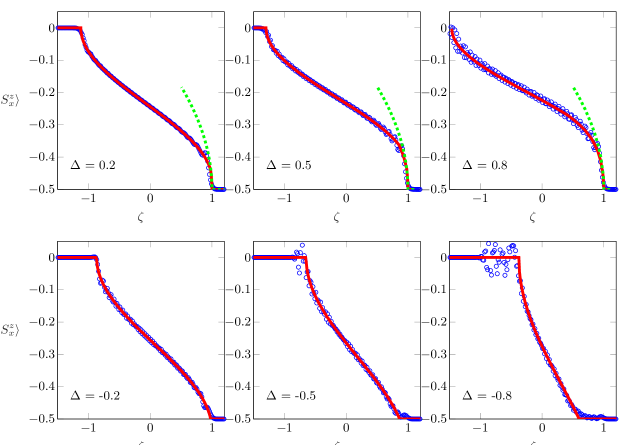
Figure 3: Magnetization profiles $\expectationvalue{S^{z}_{x}}$ after the geometric quench as a function of $\zeta=x/t$, for various values of $\Delta$. The symbols (blue) are the results of DMRG calculations, whereas the solid lines (red) are obtained from the numerical solution of the GHD ansatz. For $\Delta>0$ the approximation near the edge, Eq. (22), is shown by dashed lines (green).

III.2 Numerical results

We now present our numerical results from DMRG calculations and compare them to the $\expectationvalue{S^{z}}$ profiles as obtained from (20) by solving the GHD equations. In Fig. 3 the magnetization profiles are reported for a system with $L=200$ sites and for a fixed time $t=64$ after the quench. Instead of the lattice site $j=1,\dots,L$, we introduce the (half-integer) distance $x=j-(L+1)/2$ from the junction of the half-chains to index the sites, and plot the data $\braket{S^{z}_{x}}$ against the ray variable $\zeta=x/t$. For all the anisotropies presented, one generally observes a very good agreement between the DMRG data and the GHD solution. There are, however, some extra features that should be discussed.

First, for $\Delta>0$, the right edge of the front indeed lies at $\zeta_{max}=1$, as predicted by GHD and the ansatz (16) for the occupation provides, up to oscillations, a very good description of the edge regime. However, although the approximate solution in Eq. (22), shown by the green dashed lines in Fig. 3, seems to capture the leading behavior of the edge, its applicability is restricted to a rather small neighborhood of $\zeta=1$. As further discussed in the Appendix, this is due to the fact that the solution (21) which gives the interval of occupied rapidities actually fails to satisfy $\epsilon\ll 1$, unless $1-\zeta$ is chosen to be extremely small. In particular, $\epsilon$ diverges for $\Delta=0$ and the approximation improves as $\Delta\to 1$.

On the other hand, for $\Delta<0$, the GHD edge is given by $\zeta_{max}=\sin(\gamma)$, whereas the density can be clearly seen to extend beyond this value up to $\zeta\approx 1$. Moreover, the GHD profile shows a qualitatively different behavior around $\zeta_{max}$, where the square-root singularity seems to be replaced with a linear profile. In fact, this is very reminiscent to the case of the domain-wall initial state $\ket{\uparrow\uparrow\uparrow\dots}\otimes\ket{\downarrow\downarrow\downarrow\dots}$, where the analytical GHD profile can be obtained Collura et al. (2018) and the edge behavior has recently been investigated in detail Bulchandani and Karrasch ; Stéphan . In particular, the tail has been interpreted as a dilute regime of quasiparticles, where the interactions renormalize to zero and the edge $\zeta=1$ corresponds to the free magnon velocity Stéphan .

To have a better overview of the situation for the geometric quench, we show in Fig. 4 the magnified edge region for $\Delta=-0.8$ and various times $t$. One can see a slow decrease of the scaled profiles in the regime $\zeta_{max}<\zeta<1$, suggesting that the tail should indeed contain only a finite number of particles that could escape from the bulk of the front region. We expect that, when plotted against $\zeta$, the tail should vanish in the $t\to\infty$ limit, as the escaped density becomes smeared out in an infinitely large region. Note, however, that the results of Ref. Stéphan for the domain-wall quench are also compatible with a logarithmic increase in time of the overall number of particles in the tail regime. A detailed analysis of the tail would require much more numerical effort and is beyond the scope of the present manuscript.

One should also comment on the left edge of the profile, i.e. the front region that connects to the ground state outside the light cone. As pointed out before, the GHD ansatz suggests that the left edge should extend with the spinon velocity, i.e. the speed of the excitations above the zero-magnetization background. This seems to be in perfect accordance with the numerical data for $\Delta>0$. In the attractive ($\Delta<0$) case, however, one observes very strong oscillations beyond the GHD edge $\zeta<\zeta_{min}$. We believe that, similarly to the right edge, this feature is due to a small number of particles that escape from the attractive bulk of the front. Note also, that the GHD edge seems to have a square-root behavior for all values of $\Delta$. However, a perturbative treatment is more complicated in this case, since one has to consider the perturbation around the completely filled ground state, instead of the vacuum.

Finally, it is interesting to note that in the limit $\Delta\to-1$ one has $\zeta_{min}=\zeta_{max}=0$, and thus the bulk of the front region vanishes completely. This is a clear signal of subballistic transport in the regime $\Delta\leq-1$. On the other hand, the limit $\Delta\to 1$ shows no singular features, suggesting that the $\Delta>1$ regime is smoothly connected and the ballistic nature of the dynamics is preserved. These expectations seem to be confirmed by our DMRG numerics.

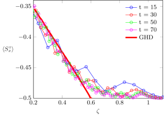
Figure 4: Edge profiles for $\Delta=-0.8$ and various times $t$, plotted against $\zeta=x/t$. The GHD solution is shown by the red solid line.

IV Entropy Profiles

The front dynamics can be further characterized by calculating the entanglement entropy $S=-\Tr\rho_{A}\ln\rho_{A}$ for a given bipartition of the chain (see Fig. 1) where $\rho_{A}$ is the corresponding reduced density matrix. The entanglement profile is obtained at a fixed time $t$ by varying the boundary between the subsystems $A=\left[1,L/2+r\right]$ and $B=\left[L/2+r+1,L\right]$. In particular, $r=0$ corresponds to a bipartition across the initial cut, the case which was already considered in Ref. Alba and Heidrich-Meisner (2014).

As opposed to the magnetization, the entanglement profile is more complicated to be captured within the hydrodynamic approach. Indeed, although there has been much progress in understanding the entropy evolution in terms of the quasiparticle picture Alba and Calabrese (2017, 2018), these results are restricted to quench scenarios where the growth is linear in time. In contrast, it has already been observed in Alba and Heidrich-Meisner (2014) that the geometric quench induces a logarithmic entropy growth for $r=0$, which is also a characteristic of local quench protocols Eisler and Peschel (2007); Eisler et al. (2008); Calabrese and Cardy (2007); Stéphan and Dubail (2011).

We first consider the noninteracting ($\Delta=0$) case where, invoking results from CFT and with some heuristic arguments, we are able to provide an ansatz for the full entanglement profile.

IV.1 XX chain

To find a quantitative description of the entropy profile, there are some features to be noted about the structure of the hydrodynamic state described above Eq. (23). First, the fermionic density $\mathcal{N}(\zeta)$ is exactly one-half of the corresponding one for a domain-wall initial state Antal et al. (1999, 2008), where the occupied modes $\left[q_{-},q_{+}\right]$ are not restricted below the Fermi-level $q_{F}=\pi/2$. Hence, the LQSS after the geometric quench is reminiscent to that of the domain-wall problem, but differs by the presence of a sharp Fermi-edge. We thus argue that the entropy can be obtained as a sum of two contributions, due to the spatially varying occupation and to the Fermi-edge singularity, respectively.

The contribution from the Fermi edge can be identified by recalling the results for the local quench, where two half-filled semi-infinite chains are joined together Calabrese and Cardy (2007). Indeed, since the initial filling is unbiased, the time evolution is entirely due to the presence of two Fermi edges at momenta $q_{F}=\pm\pi/2$. The resulting entropy profile can be obtained via CFT Calabrese and Cardy (2007) and reads

$$S_{loc}=\frac{1}{6}\ln(t^{2}-r^{2})\,,$$ (24)

where we have ignored the nonuniversal constant which is independent of both $t$ and $r$. This result can also be generalized to finite-size chains by substituting the corresponding chord-variables Stéphan and Dubail (2011)

$$t\to\frac{L}{\pi}\sin\left(\frac{\pi t}{L}\right),\quad r\to\frac{L}{\pi}\sin\left(\frac{\pi r}{L}\right).$$ (25)

It is important to stress that the result (24) and (25) gives the entropy profile resulting from two Fermi edges, whereas we need only the contribution from $q_{F}=\pi/2$, i.e. from the right-moving wavefront. Thus, using trigonometric identities we rewrite

$$S_{loc}=\frac{1}{6}\ln\left[\frac{L}{\pi}\sin\left(\frac{\pi(t-r)}{L}\right)\frac{L}{\pi}\sin\left(\frac{\pi(t+r)}{L}\right)\right],$$ (26)

which has exactly the desired additive form, with the arguments $t\mp r$ corresponding to the Fermi edges $q_{F}=\pm\pi/2$, respectively.

The second piece of contribution we have to identify is due to the space-dependent occupation. As we have already remarked, this should be closely related to the domain-wall problem, where the entropy profile is also known explicitly Eisler and Peschel (2014). In fact, the solution can be found via a curved-space CFT approach Dubail et al. (2017a), by identifying the underlying curved metric Allegra et al. (2016) and mapping it conformally onto a flat one on the upper half plane. The result can be cast in the form

$$S_{dw}=\frac{1}{6}\ln(\mathcal{L}\sin q_{F}(r/t)),$$ (27)

where the conformal length is given by

$$\mathcal{L}=t\left[1-\left(\frac{r}{t}\right)^{2}\right].$$ (28)

Note that (27) contains a nonuniversal part with $\sin q_{F}(r/t)$ being the spatially varying Fermi velocity, where $q_{F}(x)=\arccos(x)$. This term plays the role of a cutoff renormalization in the CFT picture.

We now give a heuristic argument on how to modify the expression in (27) in order to get the result for the geometric quench. As already pointed out, the fermionic density for the geometric quench is exactly the half of that in the domain-wall case, by restricting to the modes with $q\in\left[q_{-},\pi/2\right]$. Due to the particle-hole symmetry of the problem, one could also have worked with the modes $q\in\left[\pi/2,q_{+}\right]$ and arrive to the same result. Thus, assuming that the universal entropy contribution of the domain-wall problem could, in some way, be written as a sum over modes, this symmetry argument implies that the universal contribution to the geometric quench should be $\frac{1}{12}\ln\mathcal{L}$. Moreover, one should also take into account the halved density when considering the nonuniversal piece, where for the geometric quench one has $q_{F}(x)=\pi\mathcal{N}(x)=\arccos(x)/2$, such that

$$\frac{1}{6}\ln(\sin q_{F}(r/t))=\frac{1}{12}\left[\ln\left(1-\frac{r}{t}\right)-\ln 2\right].$$ (29)

Finally, collecting the different contributions, one arrives at the result

$$S_{g} =\frac{1}{6}\ln\left[\frac{L}{\pi}\sin\left(\frac{\pi(t-r)}{L}\right)\right]$$

$$+\frac{1}{12}\ln\left[(t-r)\left(1-\left(r/t\right)^{2}\right)\right]+k,$$ (30)

where $|r|<t$ and $k$ is a nonuniversal constant. In particular, setting $r=0$ one recovers the ansatz put forward in Alba and Heidrich-Meisner (2014). To test the result (30), we calculated the entropy profiles for free-fermion chains using standard correlation matrix techniques Peschel and Eisler (2009). Fig. 5 shows the result for a fixed time $t=50$ and for various chain sizes, compared to the ansatz (30) shown by solid lines. One sees a very good agreement with the numerical data. The only free parameter is the constant, which was fixed at $k\approx 0.44$ by fitting the ansatz to one of the data sets. We also carried out calculations for a larger time $t=100$ (not shown) with similarly good agreement, confirming the validity of the result in Eq. (30).

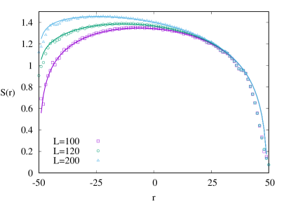
Figure 5: Entropy profiles after the geometric quench for $t=50$ and various system sizes. The solid lines correspond to the ansatz $S_{g}$ in Eq. (30). Only the front region $|r|<t$ is shown.

IV.2 XXZ chain

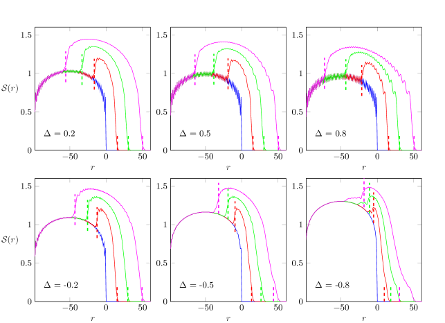
Figure 6: Entanglement profiles for different values of $\Delta$ at times $t=0$ (blue), $t=15$ (red), $t=30$ (green) and $t=50$ (magenta) after the quench. The GHD edges $r=\zeta_{min}t$ and $r=\zeta_{max}t$ are marked by vertical dashed lines.

We continue with the numerical study of the entanglement profile for the XXZ chain. In Fig. 6 the results of DMRG calculations for a chain with $L=200$ are shown. The snapshots of the profiles are plotted for various times, and the $\Delta$ values considered are the same as for the magnetization in Fig. 3. At $t=0$ (blue curve) the entanglement entropy is trivially vanishing for a cut across the right half-chain, whereas the profile on the left is given by the well-known CFT formula for the ground state Calabrese and Cardy (2004). After the quench, the entanglement spreads in both directions and a profile qualitatively similar to the XX case emerges. However, one expects that the left and right edges of the front are given by $r=\zeta_{min}t$ and $r=\zeta_{max}t$, respectively, as indicated by the dashed lines in Fig. 6. While for $\Delta>0$ this seems to hold perfectly, for $\Delta<0$ one observes, similarly to the magnetization profiles, a tail reaching beyond the GHD edges on both sides, increasing for large negative values of $\Delta$.

It is instructive to have a closer look at the right tail of the front expanding into the vacuum. As already discussed in the previous section, the tail behavior is reminiscent of the domain-wall quench where, however, the dynamics is invariant under the change of sign in $\Delta$. To emphasize the difference for the geometric quench, in Fig. 7 we compare the edge entropy profiles between $\Delta=0.8$ and $\Delta=-0.8$. While in the repulsive case the profile has a sharp edge with an abrupt increase, for the attractive one the free edge remains soft until reaching the GHD edge, where the slope becomes steep. The profile between the soft and hard edges develops a steplike structure, as can be seen for larger times in Fig. 7. In fact, beyond the left edge the profile develops a qualitatively similar tail, which can already be seen on Fig. 6 without magnifying the region.

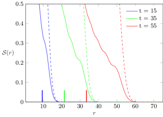
Figure 7: Comparison of the right edge of the entanglement profile for $\Delta=-0.8$ (solid lines) vs. $\Delta=0.8$ (dashed lines) and various times. The GHD edges $r=\zeta_{max}t$ for $\Delta=-0.8$ are indicated by vertical lines.

Regarding the bulk profile, it is tempting to find a generalization to the ansatz in (30). In fact, the CFT result (26) for the local quench can be applied to the XXZ case by explicitly including the spinon velocity, i.e. substituting $t\to v_{s}t$, which we have verified by DMRG calculations. On the other hand, however, the other constituent of the ansatz originates from the domain-wall quench, where the result (27) is specific to free fermions. Hence, despite the qualitatively similar behavior of the profiles, the XXZ case can not simply be related to the XX result (30) by rescaling with the front velocities.

V Boundary Effects

So far we have only considered situations where the propagating front does not reach the boundaries of the chain. Since the formulation of GHD genuinely involves the thermodynamic limit, it is interesting to ask what happens when finite size effects play a dominant role, i.e. when reflections of the wavefront occur.

V.1 XX chain

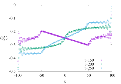
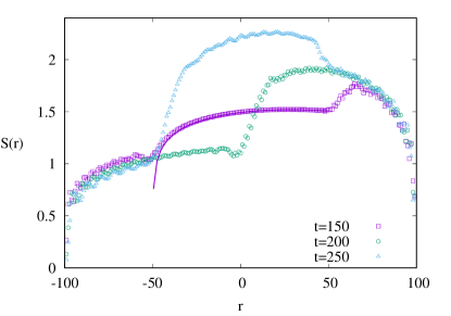
Figure 8: Magnetization (left) and entanglement (right) profiles after reflection of the wavefront from the boundaries. The solid lines show the results (23), (31) and (32) for the magnetization and (30) for the entropy, respectively.

We start again by considering the XX chain where, due to the complete independence of the quasiparticle velocities from the mode occupations, the hydrodynamic picture remains applicable even after reflections from the boundaries take place. Indeed, determining the magnetization requires only a proper bookkeeping of the contributions from the reflected particles. Considering a fixed site with $x>0$ on the r.h.s. of the chain, the result (23) remains true for times $t<L-x$, i.e. until the reflected particles with maximal velocity $v_{max}=1$ arrive there. For larger times one simply adds the contribution of the reflected density

$$\braket{S^{z}_{x}}=-\frac{1}{2}+\mathcal{N}\left(\frac{x}{t}\right)+\mathcal{N}\left(\frac{L-x}{t}\right),$$ (31)

where $L-x<t<L+x$. This last requirement ensures, that only reflections from the right end of the chain could take place.

For even larger times, one has to take into account the reflections from the left boundary. To this end one should first note, that the left-moving particles could be considered as holes penetrating the originally zero-magnetization background. This also follows directly from the exact symmetry relation $\braket{S^{z}_{-x}}$=$-1/2-\braket{S^{z}_{x}}$, which can be used to obtain the magnetization on the l.h.s. of the chain. Hence, for times $t>L+x$, the contribution of the reflected holes should appear as

$$\braket{S^{z}_{x}}=-\frac{1}{2}+\mathcal{N}\left(\frac{x}{t}\right)+\mathcal{N}\left(\frac{L-x}{t}\right)-\mathcal{N}\left(\frac{L+x}{t}\right).$$ (32)

The above result is then valid for times $L+x<t<2L-x$, i.e. until the fastest holes arrive to site $x$ after a double reflection from both left and right boundaries. Clearly, this pattern could be continued to arbitrary times after multiple reflections, always adding the fermionic density with the proper sign and argument.

The results (23), (31) and (32) are compared to exact numerical free-fermion calculations on the left of Fig. 8. One observes that, apart from oscillations, the average magnetization is well described by the semiclassical formulas. The oscillations are rather strong around the boundaries and one expects that, after many reflections, the profile becomes increasingly noisy. On the right of Fig. 8 we also plotted the corresponding entanglement profiles. As one can see, the result in (30) remains valid for that part of the profile which is not yet reached by the reflected wavefront. Interestingly, after each reflection one has a steady increase of entanglement, which was already pointed out in Alba and Heidrich-Meisner (2014) for $r=0$. Unfortunately, however, a quantitative understanding of the profile is still beyond our reach.

V.2 XXZ chain

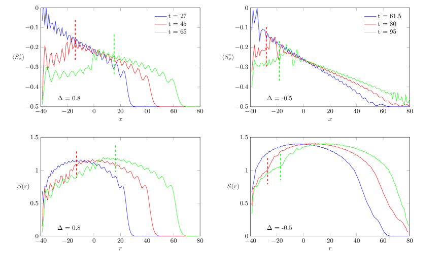
Figure 9: Magnetization (top) and entanglement (bottom) profiles for $\Delta=0.8$ (left) and $\Delta=-0.5$ (right), just before (blue) and after the reflection (red, green) of the front from the left boundary of the chain. The data is plotted against the distance from the junction. The dashed lines indicate the edge positions corresponding to a reflected front with constant speed $v_{s}$.

In contrast to the XX case, it is far from trivial how the hydrodynamic approach could be extended to include reflected quasiparticles in the interacting case. Here we try to understand only some simple qualitative features of the dynamics after reflection, focusing on the front which propagates in the l.h.s. of the system. In order to avoid interference with the reflection of the right-propagating front, for this simulation we considered a chain of size $L=L_{1}+L_{2}$, composed initially of two unequal pieces $L_{1}=40$ (ground state) and $L_{2}=80$ (vacuum).

Our results for both the magnetization and entropy profiles are shown in Fig. 9 for two different anisotropies, with the colors corresponding to different evolution times. The dashed lines indicate the calculated front positions, assuming that the speed of propagation after reflection is still given by the spinon velocity $v_{s}$. The blue curves correspond to times $t=L_{1}/v_{s}$, i.e. when the front is just supposed to reach the boundary, which is indeed what we observe in Fig. 9. In contrast, after reflection there is a clear mismatch between the calculated and the actual edge locations: the front slows down for $\Delta>0$ and speeds up for $\Delta<0$, the effect becoming more apparent for larger times. The change of speed is due to the fact, that the reflected front does not any more propagate in a zero-magnetization background, but rather in a nontrivial one left behind by the primary front. Since this background is inhomogeneous, we expect that the speed of the reflected front will actually change in time, which is supported by our numerical data. A more detailed analysis is, however, difficult due to the ambiguity in defining the edge of the reflected front, with its location getting washed out by superimposed oscillations.

Regarding the entropy evolution, one should comment on the previous observations made in Ref. Alba and Heidrich-Meisner (2014), where the following ansatz for the entropy across the junction $r=0$ for times $t\ll 2L_{2}$ was put forward

$$S(r=0)=\frac{1}{6}\ln\left[\sqrt{v_{e}t}\frac{2L_{1}}{\pi}\sin\left(\frac{\pi v_{e}t}{2L_{1}}\right)\right]+\mathrm{const}.$$ (33)

Note that this is nothing else but the XX result (30) for $r=0$ and $L=2L_{1}$, after a rescaling $t\to v_{e}t$, where the parameter $v_{e}$ was interpreted as an entanglement spreading rate. Indeed, $t=2L_{1}/v_{e}$ should correspond to the roundtrip time of the entanglement front and the speed $v_{e}$ was obtained by fitting the ansatz (33) to the data, with the result $v_{e}<v_{s}$ for $\Delta=0.5$ and $v_{e}\gtrapprox v_{s}$ for $\Delta=-0.5$ (see Fig. 12 of Ref. Alba and Heidrich-Meisner (2014)). This is in perfect accordance with our observations in Fig. 9. However, instead of being an entanglement spreading rate, the correct interpretation of $v_{e}$ is due to the modified quasiparticle velocity in the inhomogeneous background. Indeed, the very same effect appears also in the magnetization profile. Remarkably, even though the front velocity appears to be time dependent after reflection, the simple ansatz (33) was found to give a rather good description of the entropy for $t<2L_{1}/v_{e}$, with $v_{e}$ being the average roundtrip velocity.

VI Fluctuations vs. entropy

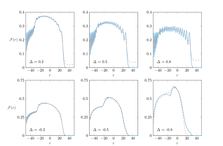
Figure 10: Comparison between the magnetization fluctuations $\mathcal{F}(r)$ (blue) and the scaled entanglement entropy $S(r)$ (red), according to Eq. (35), for a system of $L=100$ and at $t=30$.

To conclude our studies of the geometric quench, we shall consider yet another physical quantity, namely the profile of the magnetization fluctuations. Since the XXZ dynamics conserves the overall magnetization, the fluctuations are clearly vanishing for the full chain. However, considering only a segment $A$ (see Fig. 1), the subsystem fluctuations can be defined as

$$\mathcal{F}=\expectationvalue{\left(\sum_{i\in A}S^{z}_{i}-\expectationvalue{\sum_{i\in A}S^{z}_{i}}\right)^{2}},$$ (34)

where the expectation values are taken with respect to the time evolved state (2). Note that, in the fermion language, $\mathcal{F}$ is equivalent to the variance of the particle number in $A$.

For free fermion systems, the study of fluctuations is motivated by an exact relation between the ground-state entanglement entropy and the particle number statistics Klich and Levitov (2009), reproducing the entropy as a cumulant series Song et al. (2011); Calabrese et al. (2012). The scaling of the variance has thus been extensively studied in the ground state of the XX chain Eisler et al. (2006); Song et al. (2012) as well as out of equilibrium for the simple domain-wall initial state Schönhammer (2007); Antal et al. (2008). In all of the above mentioned cases one finds that, to leading order, the entropy is simply proportional to the variance, whereas the higher order cumulants give only subleading contributions.

Although the cumulant series relation between entropy and fluctuations roots deeply in the free-fermion nature of the state, there are some known extensions to interacting systems. In particular, for critical ground states described by a Luttinger liquid, the fluctuations were also found to be proportional to the entropy Song et al. (2010)

$$\mathcal{F}\simeq K\frac{3}{\pi^{2}}S+\mathrm{const}.$$ (35)

Here $K$ denotes the Luttinger parameter, while the constant is non-universal. The relation (35) has been checked explicitly for the XXZ ground state Song et al. (2010), where the Luttinger parameter is known from the Bethe ansatz solution

$$K=\frac{1}{2}\left(1-\frac{\acos(\Delta)}{\pi}\right)^{-1}.$$ (36)

However, to the best of our knowledge, no such relation has been established in an out of equlibrium context so far.

Our goal here is to study the fluctuations after the geometric quench, which can also be rewritten as a sum over correlation functions

$$\mathcal{F}=\sum_{i,j\in A}\left[\expectationvalue{S_{i}^{z}S_{j}^{z}}-\expectationvalue{S_{i}^{z}}\expectationvalue{S_{j}^{z}}\right].$$ (37)

Although these objects are straightforward to evaluate via DMRG, one needs the full matrix of correlators within the subsystem. This makes the computation somewhat more demanding, thus the simulations are now performed on a smaller chain with $L=100$ sites. The fluctuation profile $\mathcal{F}(r)$ is measured at time $t=30$, and is shown by the blue lines in Fig. 10 for a set of interaction parameters $\Delta$. The front region is clearly visible and qualitatively similar to the entropy profiles.

In order to test the relation (35) between entropy and fluctuations, we have fitted the constant for the region of the profile which corresponds to the ground state (i.e. outside the lightcone). This was done by first smoothening out the oscillations in the data and then minimizing the difference between the corresponding profiles $\mathcal{F}(r)$ and $\mathcal{S}(r)$. With the fitted constant, one can now compare the profiles in the entire front region by plotting the ansatz (35), shown by the red dashed lines in Fig. 10, together with $\mathcal{F}(r)$. Quite remarkably, the two profiles show a good agreement also within the front region, up to the superimposed oscillations. The collapse is particularly good for moderate values of $\Delta$, while for larger negative values the curves start to differ increasingly (for large $\Delta>0$ the oscillations dominate the profile and the comparison is hard).

The fact that Eq. (35) seems to give a decent approximation also in the far-from-equilibrium front region is rather intriguing, since the Luttinger parameter $K$ in Eq. (36) is calculated for the ground state. To have a better understanding of this result, one should try to analyze the behavior of correlation functions in (37), which we leave for further studies.

VII Conclusions

We have investigated the time evolution after a geometric quench in the XXZ chain and showed that the magnetization profiles are nicely captured by generalized hydrodynamics. While the entanglement profile is harder to describe within the hydrodynamic picture, we were able to put forward an ansatz for the noninteracting case which shows a very good agreement with the DMRG data.

In order to arrive at our ansatz (30), we had to apply some heuristic arguments, expressing the entropy production in the geometric quench as a kind of mixture of local and domain-wall quenches. It would be desirable to put this result on a firm ground, e.g. by a direct CFT treatment along the lines of Ref. Allegra et al. (2016), identifying the curved-space metric corresponding to the inhomogeneous time-evolved state. This might also allow for a generalization to initial states with arbitrary fillings on both sides. Ideally, however, one would like to cast the entropy as a sum over contributions from the different quasimomenta, analogously to what has been found for global quenches Alba and Calabrese (2017), which would enable us to solve the interacting problem as well. Whether such a representation is possible in situations with a logarithmic entropy growth is still unclear.

Another interesting aspect is the physics of the edge, which was shown Eisler and Rácz (2013); Viti et al. (2016); Perfetto and Gambassi (2017); Kormos (2017); Fagotti (2017) to display a universal Tracy-Widom scaling Tracy and Widom (1994) for free fermions. Clearly, the situation is more complicated in the interacting case, since one has a splitting between the GHD edge and the free edge. Recent studies for the domain-wall quench hint towards the possibility that the free tail is characterized by a Tracy-Widom-like $t^{1/3}$ length scale Bulchandani and Karrasch , while the GHD edge seems to spread diffusively as $t^{1/2}$ Stéphan . We believe that the vacuum edge of the geometric quench may belong to the same type of edge universality as observed for the domain wall. Additionally, however, one has another edge appearing in our problem which connects to the ground-state region and might display a different type of behavior. A detailed study of these edge phenomena requires much more numerical effort and is left for future studies.

Finally, it would be illuminating to understand how the presence of boundaries could be reconciled with the theory of generalized hydrodynamics. One feature we observed is that the edge velocity becomes time dependent after reflection, due to propagation in a nontrivial inhomogeneous background. Whether a quantitative description of the reflected front is possible along the lines of GHD is an interesting question to be addressed.

*

Appendix A Perturbative calculation of the edge around $\zeta_{max}$

As discussed in the main text, for $\Delta>0$ the GHD solution around the rightmost ray $\zeta_{max}=1$ is given by the occupation function (16) by solving (17). We assume that, sufficiently close to the GHD edge, the interval $\left[\lambda_{1},\lambda_{2}\right]$ of occupied rapidities remains small, i.e. $|\lambda_{1,2}-\tilde{\lambda}|\ll 1$ with $\tilde{\lambda}$ given by (15). For such an occupation, the dressing of a function $f$ can be considered as a perturbation around its bare value

$$f^{dr}(\lambda)\approx f(\lambda)+\delta f(\lambda)\,.$$ (38)

Inserting into the dressing equation (5) one obtains

$$f(\lambda)+\delta f(\lambda)+\int_{\lambda_{1}}^{\lambda_{2}}\frac{\differential\mu}{2\pi}\mathcal{K}(\lambda-\mu)\left[f(\mu)+\delta f(\mu)\right]=f(\lambda)\,.$$ (39)

To extract the leading order in the perturbation series, we neglect the term $\delta f$ within the integral and expand all the functions to first order in $\nu=\lambda-\mu$, which leaves us with

$$\delta f(\lambda)+\int_{\lambda-\lambda_{2}}^{\lambda-\lambda_{1}}\frac{\differential\,\nu}{2\pi}\left(\mathcal{K}(0)+\nu\mathcal{K}^{\prime}(0)\right)\left(f(\lambda)-\nu f^{\prime}(\lambda)\right)=0\,.$$ (40)

Setting $\lambda_{1}=\tilde{\lambda}-\epsilon_{1}$, $\lambda_{2}=\tilde{\lambda}+\epsilon_{2}$ and carrying out the integrals, we finally arrive at

$$2\pi\,\delta f(\lambda)=-\mathcal{K}(0)f(\lambda)(\epsilon_{1}+\epsilon_{2})-\left[\mathcal{K}^{\prime}(0)f(\lambda)-\mathcal{K}(0)f^{\prime}(\lambda)\right]\frac{\epsilon_{1}^{2}-\epsilon_{2}^{2}+2(\lambda-\tilde{\lambda})(\epsilon_{1}+\epsilon_{2})}{2}+\mathcal{O}(\epsilon^{3})\,.$$ (41)

With this result at hand, we can now calculate from Eq. (8) the dressed velocity

$$v\approx\frac{e^{\prime}+\delta e^{\prime}}{p^{\prime}+\delta p^{\prime}}\approx\frac{e^{\prime}}{p^{\prime}}\left[1+\frac{\delta e^{\prime}}{e^{\prime}}-\frac{\delta p^{\prime}}{p^{\prime}}+\left(\frac{\delta p^{\prime}}{p^{\prime}}\right)^{2}-\left(\frac{\delta e^{\prime}}{e}\right)\left(\frac{\delta p^{\prime}}{p^{\prime}}\right)\right],$$ (42)

where we have droppped the arguments $\lambda$. Applying (41) for both $\delta e^{\prime}$ and $\delta p^{\prime}$ and keeping only up to quadratic terms in $\epsilon_{1,2}$, one has

$$v\approx v_{0}\left[1+\frac{\mathcal{K}(0)}{2\pi}\left(\frac{e^{\prime\prime}}{e^{\prime}}-\frac{p^{\prime\prime}}{p^{\prime}}\right)\frac{\epsilon_{1}^{2}-\epsilon_{2}^{2}+2(\lambda-\tilde{\lambda})(\epsilon_{1}+\epsilon_{2})}{2}\right],$$ (43)

where $v_{0}$ is the bare velocity, see Eq. (13). The correction to the bare velocity depends on the ratios of second and first derivatives of the energy and momentum. Since the factor multiplying them is already quadratic in $\epsilon_{1,2}$, it is enough to evaluate the ratios at $\lambda=\tilde{\lambda}$. Interestingly, however, a simple calculation leads to the result

$$\evaluated{\frac{e^{\prime\prime}}{e^{\prime}}}_{\lambda=\tilde{\lambda}}=\evaluated{\frac{p^{\prime\prime}}{p^{\prime}}}_{\lambda=\tilde{\lambda}}.$$ (44)

Hence, to leading order, the velocity around the edge is just given by its bare value, with corrections $\mathcal{O}(\epsilon^{3})$. The rapidities $\lambda_{1,2}$ then follow from the condition $v_{0}(\lambda_{1})=v_{0}(\lambda_{2})=\zeta$. Expanding the bare velocity around $\tilde{\lambda}$ gives

$$v_{0}(\tilde{\lambda}\pm\epsilon)\approx v_{0}(\tilde{\lambda})\pm\epsilon v^{\prime}_{0}(\tilde{\lambda})+\frac{\epsilon^{2}}{2}v^{\prime\prime}_{0}(\tilde{\lambda})\,.$$ (45)

However, as discussed in the main text, $\tilde{\lambda}$ is exactly the maximum of the bare velocity, $v^{\prime}_{0}(\tilde{\lambda})=0$, with its value given by $v_{0}(\tilde{\lambda})=1$. Furthermore, the second derivative can be calculated as $v^{\prime\prime}_{0}(\tilde{\lambda})=-\cot^{2}(\gamma)$ and thus we get

$$v_{0}(\tilde{\lambda}\pm\epsilon)=1-\frac{\epsilon^{2}}{2}\cot^{2}(\gamma)=\zeta\,.$$ (46)

Solving for $\epsilon$ then leads to the result

$$\epsilon=\sqrt{2(1-\zeta)}\tan(\gamma)\,,$$ (47)

reported in Eq. (21) of the main text.

It should be stressed that, for the perturbation theory to work, the condition $\epsilon\ll 1$ must be satisfied. From (47) one can see that this becomes problematic, as the interaction strength is decreased. Indeed, for $\Delta\to 0$ ($\gamma\to\pi/2$) one has $\epsilon\to\infty$, i.e. the solution diverges. The reason is that for very small interactions, the bare velocity develops only a very tiny maximum around extremely high rapidities $\tilde{\lambda}\gg 1$, thus deteriorating the quality of the approximation. In particular, at the free-fermion point $\Delta=0$ the approximation fails completely, which can also be seen by expanding the analytical result (23) for the magnetization profile around $\zeta=1$. This gives to leading order

$$\braket{S^{z}}\approx-\frac{1}{2}+\frac{1}{2\pi}\sqrt{2(1-\zeta)},$$ (48)

where the coefficient of the square-root is off by a factor of $2$ with respect to the approximation (22). Moreover, even considering a larger value $\Delta=0.8$ and requiring $\epsilon<0.1$, one has from (47) the condition $\zeta>0.99$. This explains why the approximate profile deviates essentially immediately from the GHD solution in Fig. 3.

On the other hand, one expects that the edge approximation should perform much better for $\Delta\to 1$, i.e. around the isotropic Heisenberg point. This is indeed what we observe by comparing it to the numerical solutions $\lambda_{1}$ and $\lambda_{2}$ of the GHD ansatz (17). This is shown in the left of Fig. 11 for $\Delta=0.95$, where the approximation appears to be rather good around the edge but deviates as one moves further away. On the right of Fig. 11 we also show the edge profile for the magnetization, comparing the GHD solution to the approximation (22) and to the tDMRG data for $L=200$ and $t=60$.

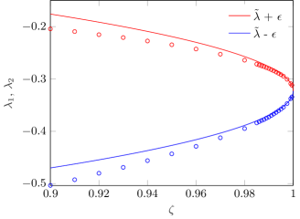
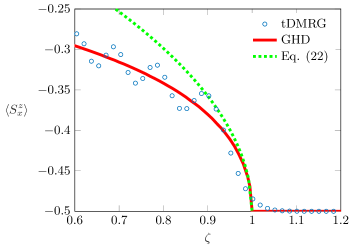
Figure 11: Left: rapidities $\lambda_{1}$ (blue circles) and $\lambda_{2}$ (red circles) as obtained from the iterative numerical solution of Eq. (17) for $\Delta=0.95$. The approximate solutions are shown by solid lines, see Eq. (47), with a good agreement near $\zeta=1$. Right: corresponding edge magnetization profile and its approximation.

References

- Polkovnikov et al. (2011) A. Polkovnikov, K. Sengupta, A. Silva, and M. Vengalattore, Rev. Mod. Phys. 83, 863 (2011).
- Gogolin and Eisert (2016) C. Gogolin and J. Eisert, Rep. Prog. Phys. 79, 056001 (2016).
- Calabrese et al. (2016) P. Calabrese, F. H. L. Essler, and G. Mussardo, J. Stat. Mech. 064001 (2016).
- Essler and Fagotti (2016) F. H. L. Essler and M. Fagotti, J. Stat. Mech. 064002 (2016).
- Vidmar and Rigol (2016) L. Vidmar and M. Rigol, J. Stat. Mech. 064007 (2016).
- Vasseur and Moore (2016) R. Vasseur and J. E. Moore, J. Stat. Mech. 064010 (2016).
- Bertini et al. (2016) B. Bertini, M. Collura, J. De Nardis, and M. Fagotti, Phys. Rev. Lett. 117, 207201 (2016).
- Castro-Alvaredo et al. (2016) O. A. Castro-Alvaredo, B. Doyon, and T. Yoshimura, Phys. Rev. X 6, 041065 (2016).
- Piroli et al. (2017) L. Piroli, J. De Nardis, M. Collura, B. Bertini, and M. Fagotti, Phys. Rev. B 96, 115124 (2017).
- Doyon and Yoshimura (2017) B. Doyon and T. Yoshimura, SciPost Phys. 2, 014 (2017).
- Doyon et al. (2017a) B. Doyon, H. Spohn, and T. Yoshimura, Nucl. Phys. B 926, 570 (2017a).
- Doyon et al. (2017b) B. Doyon, J. Dubail, R. Konik, and T. Yoshimura, Phys. Rev. Lett. 119, 195301 (2017b).
- (13) J.-S. Caux, B. Doyon, J. Dubail, R. Konik, and T. Yoshimura, arXiv:1711.00873.
- Bulchandani et al. (2017) V. B. Bulchandani, R. Vasseur, C. Karrasch, and J. E. Moore, Phys. Rev. Lett. 119, 220604 (2017).
- Bulchandani et al. (2018) V. B. Bulchandani, R. Vasseur, C. Karrasch, and J. E. Moore, Phys. Rev. B 97, 045407 (2018).
- Ilievski and De Nardis (2017) E. Ilievski and J. De Nardis, Phys. Rev. B 96, 081118(R) (2017).
- Doyon et al. (2018) B. Doyon, T. Yoshimura, and J.-S. Caux, Phys. Rev. Lett. 120, 045301 (2018).
- Mazza et al. (2018) L. Mazza, J. Viti, M. Carrega, D. Rossini, and A. De Luca, Phys. Rev. B 98, 075421 (2018).
- Mestyán et al. (2019) M. Mestyán, B. Bertini, L. Piroli, and P. Calabrese, Phys. Rev. B 99, 014305 (2019).
- Misguich et al. (2017) G. Misguich, K. Mallick, and P. L. Krapivsky, Phys. Rev. B 96, 195151 (2017).
- Ljubotina et al. (2017) M. Ljubotina, M. Znidaric, and T. Prosen, Nature Comm. 8, 16117 (2017).
- Stéphan (2017) J.-M. Stéphan, J. Stat. Mech. 103108 (2017).
- Collura et al. (2018) M. Collura, A. De Luca, and J. Viti, Phys. Rev. B 97, 081111(R) (2018).
- De Nardis et al. (2018) J. De Nardis, D. Bernard, and B. Doyon, Phys. Rev. Lett. 121, 160603 (2018).
- Calabrese and Cardy (2005) P. Calabrese and J. L. Cardy, J. Stat. Mech. P04010 (2005).
- Alba and Calabrese (2017) V. Alba and P. Calabrese, Proc. Natl. Acad. Sci. 114, 7947 (2017).
- Alba and Calabrese (2018) V. Alba and P. Calabrese, SciPost Phys. 4, 017 (2018).
- Alba (2018) V. Alba, Phys. Rev. B 97, 245135 (2018).
- Bertini et al. (2018) B. Bertini, M. Fagotti, L. Piroli, and P. Calabrese, J. Phys. A: Math. Theor. 51, 39LT01 (2018).
- Gobert et al. (2005) D. Gobert, C. Kollath, U. Schollwöck, and G. Schütz, Phys. Rev. E 71, 036102 (2005).
- Eisler et al. (2009) V. Eisler, F. Iglói, and I. Peschel, J. Stat. Mech. P02011 (2009).
- Sabetta and Misguich (2013) T. Sabetta and G. Misguich, Phys. Rev. B 88, 245114 (2013).
- Eisler and Peschel (2014) V. Eisler and I. Peschel, J. Stat. Mech. P04005 (2014).
- Dubail et al. (2017a) J. Dubail, J-M. Stéphan, J. Viti, and P. Calabrese, SciPost Phys. 2, 002 (2017a).
- Dubail et al. (2017b) J. Dubail, J-M. Stéphan, and P. Calabrese, SciPost Phys. 3, 019 (2017b).
- Eisler and Bauernfeind (2017) V. Eisler and D. Bauernfeind, Phys. Rev. B 96, 174301 (2017).
- Eisler et al. (2016) V. Eisler, F. Maislinger, and H. G. Evertz, SciPost Phys. 1, 014 (2016).
- Eisler and Maislinger (2018) V. Eisler and F. Maislinger, Phys. Rev. B 98, 161117(R) (2018).
- Mossel et al. (2010) J. Mossel, G. Palacios, and J.-S. Caux, J. Stat. Mech. L09001 (2010).
- Alba and Heidrich-Meisner (2014) V. Alba and F. Heidrich-Meisner, Phys. Rev. B 90, 075144 (2014).
- Takahashi (1999) M. Takahashi, Thermodynamics of One-Dimensional Solvable Models (Cambridge University Press, 1999).
- Franchini (2017) F. Franchini, An Introduction to Integrable Techniques for One-Dimensional Quantum Systems, vol. Lecture Notes in Physics Vol. 940 (Springer, 2017).
- Giamarchi (2003) T. Giamarchi, Quantum Physics in One Dimension (Clarendon Press, Oxford, 2003).
- Atkinson and Shampine (2008) K. E. Atkinson and L. F. Shampine, ACM Trans. Math. Softw. 34, 21 (2008).
- Schollwöck (2011) U. Schollwöck, Annals of Physics 326, 96 (2011).
- (46) ITensor library, http://itensor.org/.
- (47) V. B. Bulchandani and C. Karrasch, arXiv:1810.08227.
- (48) J.-M. Stéphan, arXiv:1901.02770.
- Eisler and Peschel (2007) V. Eisler and I. Peschel, J. Stat. Mech. P06005 (2007).
- Eisler et al. (2008) V. Eisler, D. Karevski, T. Platini, and I. Peschel, J. Stat. Mech. P01023 (2008).
- Calabrese and Cardy (2007) P. Calabrese and J. Cardy, J. Stat. Mech. P10004 (2007).
- Stéphan and Dubail (2011) J.-M. Stéphan and J. Dubail, J. Stat. Mech. P08019 (2011).
- Antal et al. (1999) T. Antal, Z. Rácz, A. Rákos, and G. M. Schütz, Phys. Rev. E 59, 4912 (1999).
- Antal et al. (2008) T. Antal, P. L. Krapivsky, and A. Rákos, Phys. Rev. E 78, 061115 (2008).
- Allegra et al. (2016) N. Allegra, J. Dubail, J-M. Stéphan, and J. Viti, J. Stat. Mech. 053108 (2016).
- Peschel and Eisler (2009) I. Peschel and V. Eisler, J. Phys. A: Math. Theor. 42, 504003 (2009).
- Calabrese and Cardy (2004) P. Calabrese and J. L. Cardy, J. Stat. Mech. P06002 (2004).
- Klich and Levitov (2009) I. Klich and L. Levitov, Phys. Rev. Lett. 102, 100502 (2009).
- Song et al. (2011) H. F. Song, C. Flindt, S. Rachel, I. Klich, and K. L. Hur, Phys. Rev. B 83, 161408(R) (2011).
- Calabrese et al. (2012) P. Calabrese, M. Mintchev, and E. Vicari, EPL 98, 20003 (2012).
- Eisler et al. (2006) V. Eisler, Ö. Legeza, and Z. Rácz, J. Stat. Mech. P11013 (2006).
- Song et al. (2012) H. F. Song, S. Rachel, C. Flindt, I. Klich, N. Laflorencie, and K. Le Hur, Phys. Rev. B 85, 035409 (2012).
- Schönhammer (2007) K. Schönhammer, Phys. Rev. B 75, 205329 (2007).
- Song et al. (2010) H. F. Song, S. Rachel, and K. Le Hur, Phys. Rev. B 82, 012405 (2010).
- Eisler and Rácz (2013) V. Eisler and Z. Rácz, Phys. Rev. Lett. 110, 060602 (2013).
- Viti et al. (2016) J. Viti, J-M. Stéphan, J. Dubail, and M. Haque, Europhys. Lett. 115, 40011 (2016).
- Perfetto and Gambassi (2017) G. Perfetto and A. Gambassi, Phys. Rev. E 96, 012138 (2017).
- Kormos (2017) M. Kormos, SciPost Phys. 3, 020 (2017).
- Fagotti (2017) M. Fagotti, Phys. Rev. B 96, 220302(R) (2017).
- Tracy and Widom (1994) C. A. Tracy and H. Widom, Commun. Math. Phys. 159, 151 (1994).