Extra-tidal structures around the Gaia Sausage candidate globular cluster NGC 6779 (M56)
Abstract
We present results on the stellar density radial profile of the outer regions of NGC 6779, a Milky Way globular cluster recently proposed as a candidate member of the Gaia Sausage structure, a merger remnant of a massive dwarf galaxy with the Milky Way. Taking advantage of the Pan-STARRS PS1 public astrometric and photometric catalogue, we built the radial profile for the outermost cluster regions using horizontal branch and main sequence stars, separately, in order to probe for different profile trends because of difference stellar masses. Owing to its relatively close location to the Galactic plane, we have carefully treated the chosen colour-magnitude regions properly correcting them by the amount of interstellar extinction measured along the line-of-side of each star, as well as cleaned them from the variable field star contamination observed across the cluster field. In the region spanning from the tidal to the Jacobi radii the resulting radial profiles show a diffuse extended halo, with an average power law slope of -1. While analysing the relationships between the Galactocentric distance, the half-mass density, the half-light radius, the slope of the radial profile of the outermost regions, the internal dynamical evolutionary stage, among others, we found that NGC 6779 shows structural properties similar to those of the remaining Gaia Sausage candidate globular clusters, namely, they are massive clusters ( 105M⊙) in a moderately early dynamical evolutionary stage, with observed extra-tidal structures.
keywords:
techniques: photometric – globular clusters: individual: NGC 6779.1 Introduction
Recently, Myeong et al. (2018) performed a search of Milky Way globular clusters (MW GCs) that possibly belong to the Gaia Sausage, an elongated structure in velocity space created by a massive dwarf galaxy ( 51010 M⊙) on a strongly radial orbit that merged with the MW at a redshift 3 (Belokurov et al., 2018). They listed NGC 1851, 1904, 2298, 2808, 5286, 6779, 6864 and 7089 as probable candidate GCs, and NGC 362 and 1261 as possible ones.
Because of the merger event that gave rise to the Gaia Sausage, these GCs are expected to have evidence of strong tidal interactions, such as long tidal tails, azimuthally irregular stellar halos, clumpy extended structures, etc. Indeed, 8 out of the 10 candidate GCs have previous studies of their outer regions and all of them show some of the above mentioned signatures. For instance, Carballo-Bello et al. (2018) found tidal tails around NGC 1851, 1904, 2298 and 2808; Carballo-Bello et al. (2012) maped the extended envelopes of NGC 1261 and 6864; Vanderbeke et al. (2015) and Kuzma et al. (2016) detected extra-tidal structures in NGC 362 and NGC 7089, respectively.
As far as we are aware, NGC 6779 (M56) has not been targeted for any analysis of its stellar structure beyond its tidal radius. However, given that almost all the Gaia Sausage candidate GCs exhibit extra-tidal features, one would also expect to find some sort of structures around NGC 6779. Precisely, the main aim of this work consists in tracing for the first time the stellar density radial profile of the outermost cluster regions, and assess on that resulting profile the membership of NGC 6779 to Gaia Sausage. For the sake of the reader, we list in Table 1 the adopted values for some pertinent cluster astrophysical properties.
The paper is organised as follows: In Section 2 we describe the observational data set used and the reddening corrections performed in order to get intrinsic magnitudes and colours. Section 3 deals with the construction of stellar radial profiles for cluster horizontal branch (HB) and main sequence (MS) stars, respectively, while in Section 4 we analyse and discuss the resulting radial profiles. Finally, Section 5 summarises the main conclusions of this work.
| Parameter | Value | Ref. |
|---|---|---|
| True distance modulus | = 15.20.1 mag | 3,4 |
| Heliocentric distancea | d = 10.960.50 kpc | |
| Core radius | = 0.44 (1.40 pc) | 1,2 |
| Half-light radius | = 1.12 (3.57 pc) | 2 |
| Tidal radius | = 10.55 (33.63 pc) | 1 |
| Jacoby radius | = (23.401.79) (74.605.71 pc) | 6 |
| Ellipticity | = 0.03 | 1 |
| Mass | = (2.810.52)105M⊙ | 2 |
| Density inside | = 138.0 M⊙/pc3 | 2 |
| Age | = 12.750.50 Gyr | 7 |
| Relaxation time | = 3.1 Gyr | 2 |
| Metallicity | [Fe/H] = -2.00.1 dex | 1,5 |
Ref.: (1) Harris (1996); (2) Baumgardt &
Hilker (2018); (3) Sarajedini
et al. (2007);
(4) Khamidullina et al. (2014); (5) Carretta et al. (2009);
(6) Balbinot &
Gieles (2018); (7) VandenBerg et al. (2013).
a computed from .
2 Observational data
With the aim of looking for extended stellar structures around NGC 6779, we made use of the public astrometric and photometric catalogue produced by the Panoramic Survey Telescope and Rapid response System (Pan-STARRS PS1 Chambers et al., 2016), which enabled us to homogeneously cover with deep photometry a large sky area. We downloaded positions (R.A. and Dec.) and PSF photometry for 2365154 stars distributed in a box of 33 centred on the cluster. We used as quality indicators the errors of the PSF magnitudes gMeanPSFMagErr and rMeanPSFMagErr to be within the ranges used by Piatti (2018) (see also error bars in Fig. 2).
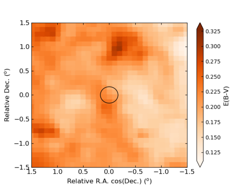
We first examined the spatial variation of the interstellar reddening across the field containing the cluster. For each entry in our Pan-STARRS PS1 catalogue, we obtained the value from Schlafly & Finkbeiner (2011) provided by NASA/IPAC Infrared Science Archive111https://irsa.ipac.caltech.edu/, which is the recalibrated MW extinction map of Schlegel et al. (1998). We derived a mean colour excess of = 0.210.04 mag for the 2365154 stars distributed in the 33 field, with lower and upper limits of 0.111 and 0.328 mag, respectively. For a circular region centred on NGC 6779, we obtained = 0.200.03 from 31833 stars located within , with lower and upper values of 0.139 and 0.249 mag, respectively. This means that this field is affected by a relative low interstellar absorption, with a slight differential reddening. Fig. 1 illustrates the spatial distribution of values.
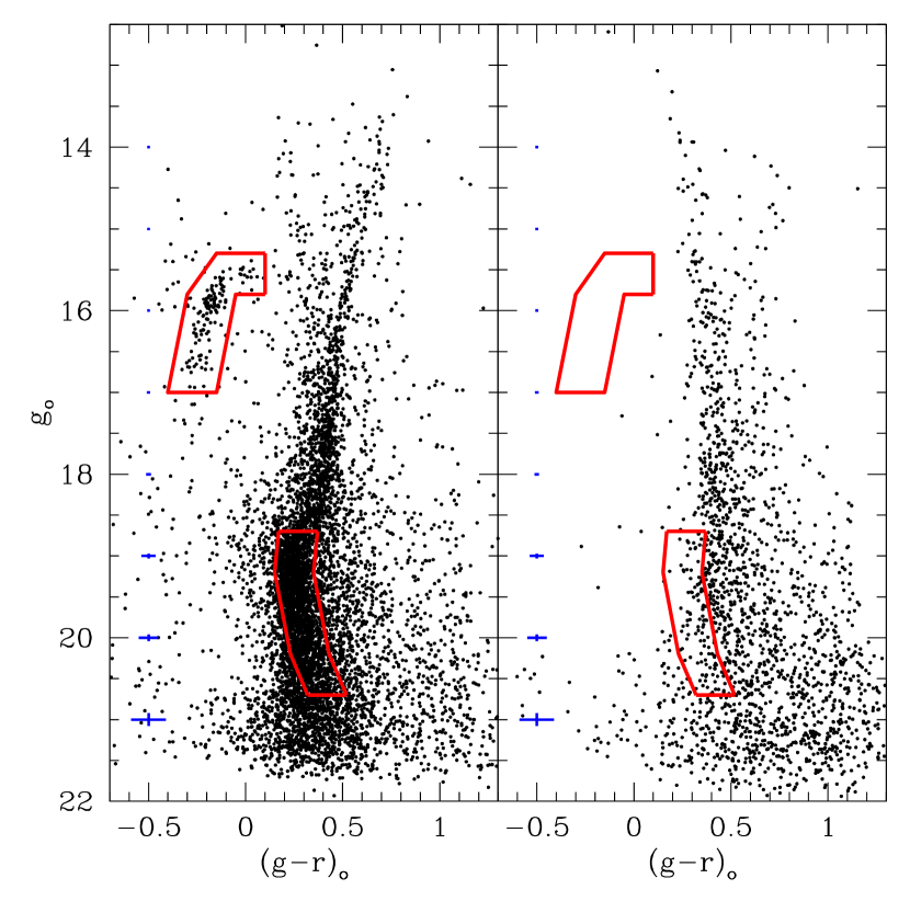
Then, we derived intrinsic magnitudes and colours from the Pan-STARRS PS1 magnitudes by correcting them for interstellar absorption, using the individual values and the / coefficients given by Tonry et al. (2012). Aiming at illustrating the wealth of information we gathered, Fig. 2 depicts the intrinsic colour-magnitude diagram (CMD) of the inner cluster region ( 5) and that of a sky region with equivalent area located at 1 towards the north-west.
3 stellar radial profiles
To trace the stellar density radial profile of the outermost regions of NGC 6779 we considered cluster HB and MS stars as illustrated in Fig. 2, where both groups of stars have been delineated with red contour lines. HB stars were initially chosen because they are practically not contaminated by the foreground field, as judged by the absence of them in the CMD of the comparison star field located at 1 to the north-west from the cluster centre. Similar HB strips result from any selected comparison star field.
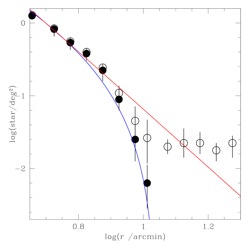
We then built the cluster HB density radial profile by applying a kernel density estimator (KDE) technique. Particularly, we employed the KDE routine within AstroML (Vanderplas et al., 2012), which has the advantage of not depending on the bin size and starting point. KDE also estimates the optimal FWHM of the Gaussians fitted in a generated grid of 750750 cells throughout the 33 field to build the stellar density map. The radial profile was then obtained by averaging the generated stellar density values for annular regions of log(r /arcmin)= 0.05 wide. The resulting stellar density profile is shown in Fig. 3 with open circles, with the respective error bars. From it, the mean background level was estimated by averaging those values for log(r /arcmin) 1.1 and subtracted from the measured stellar density profile. The background subtracted profile is depicted with filled circles in Fig. 3. In this case, the error bars come from considering in quadrature the uncertainties of the measured density profile and the dispersion of the background level. For comparison purposes, we have overplotted the curves corresponding to the King (1962) and Plummer (1911) models using the , and values of Table 1.
As for the radial profile from MS stars, we defined a strip from the cluster MS turnoff down to 2 mags, that expands magnitudes and colours in the ranges (18.7,20.7) and (0.15,0.52), respectively. We decided to go as deep as to be within 100 per cent of the photometry completeness; the 50 per cent photometry completeness being at == 23.2 mag, determined with PSF photometry of stellar sources in the stacked images (Farrow et al., in preparation).
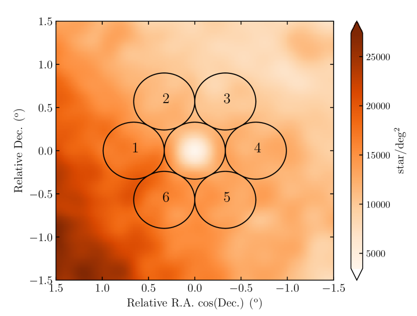
Unlike the HB strip, the MS one is noticeably contaminated by field stars, as can be seen in the CMD for the comparison star field of Fig. 2. Furthermore, the stellar density and the magnitude and colour distributions of stars in that strip vary with the position around NGC 6779. Indeed, we built a stellar density map with all these stars using the KDE that visibly reveals these variations. Fig. 4 depicts the resulting density map, where we have excluded the inner cluster region () in order to highlight the field density inhomogeneities. The clear density gradient along the south-east north-west direction is due to the position of NGC 6779 in the MW (l= 62.66, b=+8.34) rather than from reddening fluctuations. This makes the analysis of the cluster outer regions more challenging, because we first need to statistically clean the cluster MS strip from the field star contamination before building the cluster radial profile. Should we first build the stellar density profile from the observed cluster MS strip stars, would not allow us afterwards to obtain a background subtracted one – as we could satisfactorily do for HB stars –, because the background level around the cluster is not reasonably uniform for MS strip stars.
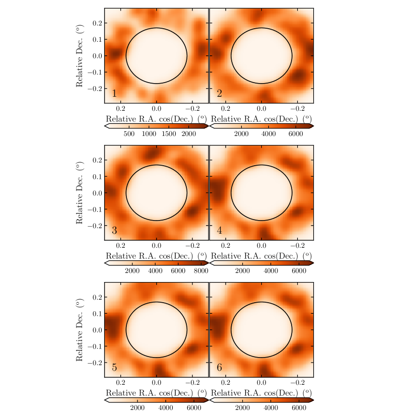
In performing the cleaning of the cluster CMD MS strip we considered a circle around the cluster centre with radius . We also defined 6 different circular star field regions distributed around the cluster area of equal size as the cluster circle; we have labelled them with numbers 1 to 6 (see Fig. 4). The mean stellar densities of these 6 star field regions turned out to be: 16448421, 11687439, 9790536, 12085349, 13368363 and 15762261 star/deg2, respectively. Since none of the field areas are representative of that along the line-of-sight of the cluster, our strategic approach consisted in decontaminating the cluster MS strip using the 6 different reference star fields at a time, and then evaluating the statistical significance of any residual structure that might arise from the 6 cleaned CMD MS strips. Thus, we compensate cleaning executions using reference star fields less and more dense than that along the line-of-sight of the cluster. Notice that we cleaned the cluster area out to its . In order to extent the cleaning towards farther regions, we would even need to use comparison fields located at larger distances from the clustes, which would make in turn the outcomes more unreliable. Our selected reference star fields are located far enough from the cluster region, but not too far as to lose the local distribution in stellar density, magnitude and colour of MW stars.
For each reference star field CMD, we generated a sample of boxes (,) centred on each star, with sizes (,) defined in such a way that one of their corners coincides with the closest star in that CMD region. This procedure of representing the reference star field CMD like an assembly of boxes was developed by Piatti & Bica (2012) and successfully used elsewhere (see, e.g, Piatti, 2017a, b; Piatti et al., 2018). It has the advantage of accurately reproducing the reference star field in terms of stellar density, luminosity function and colour distribution. This is because the number of assembled boxes is equal to the number of stars in the reference star field CMD, as well as the distribution of the magnitudes and colours of the box centres.
The generated box sample of each reference star field CMD was superimposed at a time to the cluster CMD and subtracted from it one star per box; that closest to the box centre. The resulting cleaned CMD - one per field star CMD used - contains mainly cluster members, although some negligible amount of interlopers can be expected. If the reference star field does not represent that along the line-of-sight of the cluster, the resulting cleaned cluster CMD is therefore less representative of cluster intrinsic features. Because of the variation in the stellar density around of the cluster area, we expect some difference between the reference star field and that along the line-of-sight of the cluster, that can blur the actual cluster features. For this reason, we compared the 6 different stellar radial profiles prior to draw any conclusion about the existence of extra-tidal cluster tracers (see Section 4).
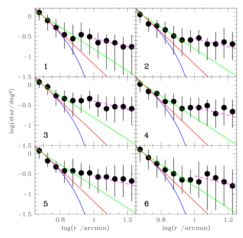
The star field cleaned radial profiles were built similarly to that for HB stars, i.e, by producing stellar density maps with the KDE and then by averaging all the stellar density values inside annuli of log(r /arcmin)= 0.05. For instance, for the annulus centred at log(r /arcmin)= 0.425, we used 108 values, while at log(r /arcmin)= 1.225, we averaged 3540 points. Fig. 5 shows the 6 different resulting radial profiles. Each panel is labelled with the number of the respective reference star field. We have overplotted King (1962), Plummer (1911) and Elson et al. (1987) models with blue, red and light-green curved lines, respectively. For the Elson et al. (1987) model, we used the value of Table 1 and our best-fitted value = 2.70.2. Additionally, we overplotted for the outermost region a power law with a slope = -1, using a magenta dashed line. Finally, we repeated the above steps to produce azimuthal density profiles for stars located between and , also depicted in Fig. 5.

4 Analysis and discussion
At first glance, Fig. 3 shows that HB stars seem to be tidally filled, with not hint for extended structures beyond . Note that not only the observed radial profile satisfactorily follows a King (1962) model, but also that the adopted and values (see Table 1) represent very well the cluster HB density radial profile. The lack of evidence of extra-tidal features from HB stars does not imply that the cluster has not been subjected to the effects of the MW gravitational potential. As pointed out by Carballo-Bello et al. (2012), stars with smaller masses can be found more easily far away from the cluster main body. For this reason, most of the studies devoted to the search for extra-tidal structures have used relatively faint MS stars (see, e.g. Olszewski et al., 2009; Saha et al., 2010; Piatti, 2017b). Additionally note that mass segregation also makes more massive stars to be more centrally concentrated (Khalisi et al., 2007, and references therein).
Indeed, the radial profiles constructed in Fig. 5 appear to reveal a different picture of NGC 6779. As can be seen, independently of the reference star field adopted to decontaminate the cluster CMD MS strip, the radial profiles exhibit noticeable excesses of stars out to . These stellar excesses appear to be important in the context of the overall cluster stellar density radial profile, as judged by the fact that a relatively small Elson et al. (1987)’s value (2.7) – very much appropriate to represent extended halos (see, e.g. Piatti, 2018, and reference therein) – is not enough to trace the outermost stellar density profiles. A power law with an average slope equal to -1 is needed to reproduce the observed trend. At this point, we can conclude from the comparison of HB and MS radial profiles, that there exists a differential mass segregation pattern, being the less massive stars significanly more segregated.
Gieles et al. (2011) distinguished from a theoretical point of view tidally affected (evaporation dominated) from tidally unaffected (expansion dominated) GCs in the half-mass density versus Galactocentric distance plane. Later, Carballo-Bello et al. (2012) reproduced such a plot for 114 GCs (see their figure1). In general, tidally unaffected GCs are massive objects ( 10), among which NGC 6779 should be included. Indeed, by using a solar Galactocentric distance () of 8.3 kpc and the cluster heliocentric distance of Table 1, we obtained = 10.32.3 kpc, which places the cluster in the half-mass density versus diagram into the region of tidally unaffected GCs. This also happens for all the remaining Gaia Sausage candidates GCs. Their masses are in the range (1.2 - 7.4)105M⊙ (Baumgardt & Hilker, 2018) and their values span from 9.4 up to 18.8 kpc Harris (1996, 2010 edition). However, most of them have been found to possess tidal tails or diffuse extended structures, thought to be evidence of past tidal interactions with the MW (see Sect. 1). If we consider Pal 5 and NGC 5466 (mass (1-4)104M⊙, (Baumgardt & Hilker, 2018)) – two low-mass GCs with evidence of massive tidal tails around them included in the sample of Carballo-Bello et al. (2012), – we conclude that the distinction between tidally affected and tidally unaffected GCs is not as straightforward as Gieles et al. (2011) suggested. Indeed, recently Webb et al. (2018) performed controlled -body simulations to systematically analyse clusters disruption by tidal shocks, and found that the amount of mass lost by the cluster depends on several factors, among them the strength of the shock, the density of the cluster within , the number of sub-shocks and the space of time between them.
Carballo-Bello et al. (2012) found that the Elson et al. (1987)’s slope can be used to discriminate between tidally affected and tidally unaffected GCs. Those tidally affected GCs not only are low-mass objects, but also have values bigger than 4. The typical value for their tidally unaffected GC sample – they show flatter profiles extending to large distances from their compact cores – is 3.00.3, in very good agreement with the value derived here for NGC 6779 (2.70.2). They also investigated the existence of any relationship of with the internal structural evolution (dynamical relaxation) and external forces (e.g., tidal shocks) using a subsample of 10 GGs with known orbits. They found that external factors are important in tidally affected GCs, while internal processes are the main mechanisms of the dynamical evolution of tidally unaffected ones. From these findings, NGC 6779 should be currently in an expansion dominated phase. However, as mentioned above, the Gieles et al. (2011)’s classification between tidally affected and tidally unaffected GCs confront with observational evidence. For instance, NGC 1851, 1904, 2298 and 2808 are GCs with observed tidal tails and values between 2.7 and 3.5 (Carballo-Bello et al., 2018).
Stronger tidal fields in the inner parts of the MW can limit the size of GCs. van den Bergh et al. (1991) investigated this phenomenon and found a correlation between GC values and the respective ones. Recently, Baumgardt & Hilker (2018) confirmed such a trend for the half-mass radii of 112 MW GCs. The resulting relationship is far from being tight (Spearman rank order coefficient of 0.490.07), revealing that tidal effects could be partially responsible of that correlation. In order to probe this effect, we searched the Harris (1996, 2010 edition) catalogue looking for MW GCs with values similar to that of NGC 6779, within the quoted uncertainty, i.e., 8.0 kpc 12.6 kpc. We found 14 GCs (NGC 288, 362, 2808, 3201, 4590, 5272, 5286, 6101, 6205, 6341, 7078, 7089, Pal 11 and E 3) with between 2.1 and 4.8 pc and an average of 4.01.4 pc, in very good agreement with the value of NGC 6779 (3.57 pc). All of them are massive objects (1.2 - 7.4 105M⊙, Baumgardt & Hilker (2018)), while seven have structural analyses of their outer regions showing a variety of extra-tidal structures, namely: NGC 288 presents an extra-tidal clumply structure that extends up to 3.5 times further than the cluster (Piatti, 2018); NGC 362 (Vanderbeke et al., 2015), NGC 4590, 5272 and 7078 (Carballo-Bello et al., 2012) show outer remarkable continuous power-law distributions extending to large distances from their compact cores; NGC 7089 exhibits a diffuse nearly circular-shaped envelope extending to 5 times the nominal cluster value (Kuzma et al., 2016) and NGC 2808 presents tails with different morphologies (Carballo-Bello et al., 2018). From this result we infer that could mislead our interpretation as tidally affected or tidally unaffected objects. Their own dynamical histories (e.g., the evolution of the eccentricity of their orbital motions, the number of tidal shocks, the in-situ or acreeted formation scenarios) could play a relevant role in shaping their structures.
According to the semi-analytical model proposed by Balbinot & Gieles (2018) for the evolution of the GC mass function in terms of its orbits coupled to a fast stellar stream, the preferencial escape of low-mass stars could explain the absence of tails near massive GCs, despite the fact that massive GCs lose stars at a higher rate. From this model, GCs with optimal detectability conditions of tidal tails are those with a low remaining mass fraction – a measure of its stage of dissolution – and a high orbital phase . The authors highlighted NGC 6779 as a candidate to have tidal tails, based on their estimated =0.25. However, this is in tension with the fact that the cluster is a massive GC. On the other hand, in the case of existing tidal tails, symmetrically collimated structures should be detected from outwards (see, e.g., Odenkirchen et al., 2001; Belokurov et al., 2006; Niederste-Ostholt et al., 2010; Sollima et al., 2011; Balbinot et al., 2011; Erkal et al., 2017; Navarrete et al., 2017; Myeong et al., 2017; Carballo-Bello et al., 2018). The right-hand panels of Fig. 5 do not show a noticeable variation of the radial profiles with the position angle beyond , but evidence of a low-density nearly azimuthally regular envelope. For the sake of the reader, Fig 6 illustrates the respective stellar density maps. Note that the appearance of some clumpy structures depends on the reference star field used.
Recently, Ferraro et al. (2018) showed that the parameter – defined as the area enclosed between the cumulative radial distribution of blue straggler stars and that of a reference population – is a powerful internal dynamical clock for MW GCs. They obtained =0.130.06 for NGC 6779, which implies that the cluster has a modest level of internal evolution. Taking this result into account we infer that the extended diffuse, nearly azimuthally regular structure found in NGC 6779 could have been caused by the effects of the MW potential, rather than dominated by internal relaxation, although evidence for tidal shocks has not been detected. Furthermore, almost all Gaia Sausage candidates GCs would not seem to be experiencing an advanced internal dynamical stage either, as judged by their estimated values, which span from 0.10 up to 0.25, with an average of 0.18 (6 GCs); NGC 1851 being the sole exception (=0.48).
5 Conclusions
NGC 6779 is among the 10 MW GCs suggested to belong to the Gaia Sausage, a structure that emerged from the accretion of a massive dwarf galaxy to the MW. Almost all candidate GC members exhibit some kind of extra-tidal feature (tails, extended halos, etc), witnesses of the strong tidal interactions that could have taken place during the merger event. The outermost regions of NGC 6779 have not been studied so far, so that it is still worth to analyse them in order to investigate whether they differ from the remaining Gaia Sausage candidate GCs.
We made use of the Pan-STARRS PS1 public astrometric and photometric catalogue to trace for the first time the outer stellar density radial profile of NGC 6779, reaching its radius. In doing that we first corrected the magnitudes of each observed star located in a field of 33 centred on the cluster according to the amount of interstellar extinction along the line-of-sight of that star. Fortunately, although the cluster is placed at a relatively low Galactic latitude, the reddening map revealed relatively small colour excesses with a relative low signature of differential reddening as well. Then, we delineated two CMD regions, one embracing the cluster HB and another along the MS, from the cluster MS turnoff down to 2 mag.
Because of the visible variation of the field star density across the cluster field, we cleaned both devised regions from field contamination by using a method that gets rid of the actual luminosity function and colour distribution of field stars from the cluster CMD. We then used the unsubtracted to build stellar density maps from an optimised KDE technique, which in turn, were used to construct the cluster radial profiles. To clean the cluster CMD we used six different reference star fields uniformly distributed around the cluster, that span all the star field scenarios, from those less dense than that along the cluster line-of-sight up to those more crowded. All the resulting radial profiles show a diffuse nearly continuos structure that extends from the cluster until its . The general trend of this extra-tidal feature can be represented by a power law with an average slope of -1. This means that the diffuse extended halo is less steep than our best-fitted Elson et al. (1987) model (= 2.7), which suggest that it could extend even further.
We made use of diagnostic diagrams proposed as good discriminators between tidally affected and tidally unaffected GCs, such as the Galactocentric distance versus half-light radius plane and the half-mass density versus Galactocentric distance diagram. We also investigated the possible origin of the extended halo from the internal dynamical clock index and the dependance of with the GC orbital parameters.
In general, we found that the link between Galactocentric distances, half-light radius, half-mass density, present-day cluster mass, orbital parameters, among others, and the origin of extra-tidal structures is not straightforward as previously thought. There are a number of issues to be considered along the lifetime of the GCs, such as the occurrence of tidal-shocks, the number and the time spacing of them, that can result in different outcomes (more or less mass lose, spatial pattern of the escaping stars, etc). In the case of NGC 6779, we found structural properties that are within the values spanned among the remaining Gaia Sausage candidates GCs. They are massive clusters ( 105M⊙), with flatter profiles extending to large distances from their compact cores ( 3.0), and internal dynamical clock index revealing a moderate evolutionary stage. Precisely, based on this latter parameter we speculate with the possibility that all the variety of extended features seen in the Gaia Sausage candidates GCs – from now NGC 6779 also included – represent the footprints of the tidal interaction with the MW.
Acknowledgements
We thank the referee for the thorough reading of the manuscript and timely suggestions to improve it. JAC-B acknowledges financial support to CAS-CONICYT 17003. The Pan-STARRS1 Surveys (PS1) and the PS1 public science archive have been made possible through contributions by the Institute for Astronomy, the University of Hawaii, the Pan-STARRS Project Office, the Max-Planck Society and its participating institutes, the Max Planck Institute for Astronomy, Heidelberg and the Max Planck Institute for Extraterrestrial Physics, Garching, The Johns Hopkins University, Durham University, the University of Edinburgh, the Queen’s University Belfast, the Harvard-Smithsonian Center for Astrophysics, the Las Cumbres Observatory Global Telescope Network Incorporated, the National Central University of Taiwan, the Space Telescope Science Institute, the National Aeronautics and Space Administration under Grant No. NNX08AR22G issued through the Planetary Science Division of the NASA Science Mission Directorate, the National Science Foundation Grant No. AST-1238877, the University of Maryland, Eotvos Lorand University (ELTE), the Los Alamos National Laboratory, and the Gordon and Betty Moore Foundation.
References
- Balbinot & Gieles (2018) Balbinot E., Gieles M., 2018, MNRAS, 474, 2479
- Balbinot et al. (2011) Balbinot E., Santiago B. X., da Costa L. N., Makler M., Maia M. A. G., 2011, MNRAS, 416, 393
- Baumgardt & Hilker (2018) Baumgardt H., Hilker M., 2018, MNRAS, 478, 1520
- Belokurov et al. (2006) Belokurov V., Evans N. W., Irwin M. J., Hewett P. C., Wilkinson M. I., 2006, ApJ, 637, L29
- Belokurov et al. (2018) Belokurov V., Erkal D., Evans N. W., Koposov S. E., Deason A. J., 2018, MNRAS, 478, 611
- Carballo-Bello et al. (2012) Carballo-Bello J. A., Gieles M., Sollima A., Koposov S., Martínez-Delgado D., Peñarrubia J., 2012, MNRAS, 419, 14
- Carballo-Bello et al. (2018) Carballo-Bello J. A., Martínez-Delgado D., Navarrete C., Catelan M., Muñoz R. R., Antoja T., Sollima A., 2018, MNRAS, 474, 683
- Carretta et al. (2009) Carretta E., Bragaglia A., Gratton R., D’Orazi V., Lucatello S., 2009, A&A, 508, 695
- Chambers et al. (2016) Chambers K. C., et al., 2016, preprint, (arXiv:1612.05560)
- Elson et al. (1987) Elson R. A. W., Fall S. M., Freeman K. C., 1987, ApJ, 323, 54
- Erkal et al. (2017) Erkal D., Koposov S. E., Belokurov V., 2017, MNRAS, 470, 60
- Ferraro et al. (2018) Ferraro F. R., et al., 2018, ApJ, 860, 36
- Gieles et al. (2011) Gieles M., Heggie D. C., Zhao H., 2011, MNRAS, 413, 2509
- Harris (1996) Harris W. E., 1996, AJ, 112, 1487
- Khalisi et al. (2007) Khalisi E., Amaro-Seoane P., Spurzem R., 2007, MNRAS, 374, 703
- Khamidullina et al. (2014) Khamidullina D. A., Sharina M. E., Shimansky V. V., Davoust E., 2014, Astrophysical Bulletin, 69, 409
- King (1962) King I., 1962, AJ, 67, 471
- Kuzma et al. (2016) Kuzma P. B., Da Costa G. S., Mackey A. D., Roderick T. A., 2016, MNRAS, 461, 3639
- Myeong et al. (2017) Myeong G. C., Jerjen H., Mackey D., Da Costa G. S., 2017, ApJ, 840, L25
- Myeong et al. (2018) Myeong G. C., Evans N. W., Belokurov V., Sanders J. L., Koposov S. E., 2018, ApJ, 863, L28
- Navarrete et al. (2017) Navarrete C., Belokurov V., Koposov S. E., 2017, ApJ, 841, L23
- Niederste-Ostholt et al. (2010) Niederste-Ostholt M., Belokurov V., Evans N. W., Koposov S., Gieles M., Irwin M. J., 2010, MNRAS, 408, L66
- Odenkirchen et al. (2001) Odenkirchen M., et al., 2001, ApJ, 548, L165
- Olszewski et al. (2009) Olszewski E. W., Saha A., Knezek P., Subramaniam A., de Boer T., Seitzer P., 2009, AJ, 138, 1570
- Piatti (2017a) Piatti A. E., 2017a, MNRAS, 465, 2748
- Piatti (2017b) Piatti A. E., 2017b, ApJ, 846, L10
- Piatti (2018) Piatti A. E., 2018, MNRAS, 473, 492
- Piatti & Bica (2012) Piatti A. E., Bica E., 2012, MNRAS, 425, 3085
- Piatti et al. (2018) Piatti A. E., Cole A. A., Emptage B., 2018, MNRAS, 473, 105
- Plummer (1911) Plummer H. C., 1911, MNRAS, 71, 460
- Saha et al. (2010) Saha A., et al., 2010, AJ, 140, 1719
- Sarajedini et al. (2007) Sarajedini A., et al., 2007, AJ, 133, 1658
- Schlafly & Finkbeiner (2011) Schlafly E. F., Finkbeiner D. P., 2011, ApJ, 737, 103
- Schlegel et al. (1998) Schlegel D. J., Finkbeiner D. P., Davis M., 1998, ApJ, 500, 525
- Sollima et al. (2011) Sollima A., Martínez-Delgado D., Valls-Gabaud D., Peñarrubia J., 2011, ApJ, 726, 47
- Tonry et al. (2012) Tonry J. L., et al., 2012, ApJ, 750, 99
- VandenBerg et al. (2013) VandenBerg D. A., Brogaard K., Leaman R., Casagrande L., 2013, ApJ, 775, 134
- Vanderbeke et al. (2015) Vanderbeke J., De Propris R., De Rijcke S., Baes M., West M. J., Blakeslee J. P., 2015, MNRAS, 450, 2692
- Vanderplas et al. (2012) Vanderplas J., Connolly A., Ivezić Ž., Gray A., 2012, in Conference on Intelligent Data Understanding (CIDU). pp 47 –54, doi:10.1109/CIDU.2012.6382200
- Webb et al. (2018) Webb J. J., Reina-Campos M., Kruijssen J. M. D., 2018, arXiv e-prints,
- van den Bergh et al. (1991) van den Bergh S., Morbey C., Pazder J., 1991, ApJ, 375, 594