A Comparison of Random Task Graph Generation Methods for Scheduling Problems

Abstract

How to generate instances with relevant properties and without bias remains an open problem of critical importance for a fair comparison of heuristics. In the context of scheduling with precedence constraints, the instance consists of a task graph that determines a partial order on task executions. To avoid selecting instances among a set populated mainly with trivial ones, we rely on properties that quantify the characteristics specific to difficult instances. Among numerous identified such properties, the mass measures how much a task graph can be decomposed into smaller ones. This property, together with an in-depth analysis of existing random task graph generation methods, establishes the sub-exponential generic time complexity of the studied problem. Empirical observations on the impact of existing generation methods on scheduling heuristics concludes our study.

1 Introduction

How to correctly evaluate the performance of computing systems has been a central question since several decades[Jai90]. Among the arsenal of available evaluation methods, relying on random instances allows comparing strategies in a large variety of situations. However, random generation methods are prone to bias, which prevents a fair empirical assessment. It is thus crucial to provide guarantees on the random distribution of generated instances by ensuring, for instance, a uniform selection of any instance among all possible ones. Yet, for some problems, such uniformly generation instances are easy to solve and thus uninteresting. For instance, in uniformly distributed random graphs, the probability that the diameter is 2 tends exponentially to 1 as the size of the graph tends to infinity[Fag76]. Studying the problem characteristics to constrain the uniform generation on a category of instances is thus critical.

In the context of parallel systems, instances for numerous multiprocessor scheduling problems contain the description of an application to be executed on a platform[Leu04]. This study focuses on scheduling problems requiring a Directed Acyclic Graph (DAG) as part of the input. Such a DAG represents a set of tasks to be executed in a specific order given by precedence constraints: the execution of any task cannot start before all its predecessors have completed their executions. Scheduling a DAG on a platform composed of multiple processors consists in assigning each task to a processor and in determining a start time for each task. While this work studies the DAG structure for several scheduling problems, it illustrates and analyzes existing generation methods in light of a specific problem with unitary costs and no communication. This simple yet difficult problem emphasizes the effect of the DAG structure on the performance of scheduling heuristics.

Some pathological instances are straightforward to solve. For instance, if the width (i.e. maximum number of tasks that may be run in parallel) is lower than the number of processors, then the problem can be solved in polynomial time. To avoid such instances, multiple DAG properties are proposed and analyzed. In particular, the mass measures the degree to which an instance can be decomposed into smaller independent sub-instances. In the absence of communication, this property has an impact on scheduling algorithms. The purpose of this work is to identify such properties to determine how the uniform generation of DAGs should be constrained and how existing generation methods perform relatively to these properties. As a major contribution of this work, we determine the generic time complexity to be sub-exponential for uniform instances for a large class of scheduling problems (i.e. those that can be decomposed into smaller problems).

After exposing related works in Section 2, Section 3 lists DAG properties and covers scheduling and random generation concepts. Section 4 motivates the focus on a selection of properties by analyzing all the proposed DAG properties on a set of special DAGs. Section 5 provides an in-depth analysis of existing random DAG generation methods supported by consistent empirical observations. Finally, Section 6 studies the impact of these methods and the DAG properties on scheduling heuristics. The algorithms are implemented in R and Python and the related code, data and analysis are available in[CSH19].

2 Related Work

2.1 Analysis of Generation Methods

Our approach is similar to the one followed in[CMP⁺10] and[Mar18], which consists in studying the properties of randomly generated DAGs before comparing the performance of scheduling heuristics. In[CMP⁺10], three properties are measured and analyzed for each studied generation method: the length of the longest path, the distribution of the output degrees and the number of edges. We describe 15 such properties in Table 2. They consider five random generation methods (described in this section and Section 5): two variants of the Erdős-Rényi algorithm, one layer-by-layer variant, the random orders method and the Fan-in/Fan-out method. Finally, for each generation method, the paper compares the performance of four scheduling heuristics. The results are consistent with the observations done in Section 5 (Figures 3, 6 and 9) for the length and the number of edges. A similar approach is undertaken in[Mar18]. First, three characteristics are considered: the number of vertices in the critical path, the width (or maximum parallelism) and the density of the DAG in terms of edges. These characteristics are studied on DAGs generated by two main approaches (the Erdős-Rényi algorithm and a MCMC approach) with sizes between 5 and 30 vertices. Finally, although no DAG property is studied, scheduling heuristics are compared using a variety of random and non-random DAGs in[KA99].

We describe below generation tools, data sets and random generation methods.

2.2 Generation Tools

Many tools have been proposed in the literature to generate DAGs in the context of scheduling in parallel systems. TGFF (Task Graphs For Free) is the first tool proposed for this purpose[DRW98]. This tool relies on a number of parameters related to the task graph structure: maximum input and output degrees of vertices, average for the minimum number of vertices, etc. The task graph is constructed by creating a single-vertex graph and then incrementally augmenting it. This approach randomly alternates between two phases until the number of vertices in the graph is greater than or equal to the minimum number of vertices: the expansion of the graph and its contraction. The main goal of TGFF is to gain more control over the input and output degrees of the tasks.

DAGGEN was later proposed to compare heuristics for a specifc problem[DNSC09]. This tool relies on a layer-by-layer approach with five parameters: the number of vertices, a width and regularity parameters for the layer sizes, and a density and jump parameters for the connectivity of the DAG. The number of elements per each layer is uniformly drawn in an interval centered around an average value determined by the width parameter and with a range determined by the regularity parameter. Lastly, edges are added between layers separated by a maximum number of layers determined by the jump parameter (edges only connect consecutive layers when this parameter is one). For each vertex, a uniform number of predecessors is added between one and a maximum value determined by the density parameter.

GGen has been proposed to unify the generation of DAGs by integrating existing methods[CMP⁺10]. The tool implements two variants of the Erdős-Rényi algorithm, one layer-by-layer variant, the random orders method and the Fan-in/Fan-out method. It also generates DAGs derived from classical parallel algorithms such as the recursive Fibonacci function, the Strassen multiplication algorithm, the Cholesky factorization, etc.

The Pegasus workflow generator can be used to generate DAGs from several scientific applications[JCD⁺13] such as Montage, CyberShake, Broadband, etc. XL-STaGe produces layer-by-layer DAGs using a truncated normal distribution to distribute the vertices to the layers[CDB⁺16]. This tool inserts edges with a probability that decreases as the number of layers between two vertices increases. A tool named RandomWorkflowGenerator implements a layer-by-layer variant[GCJ17]. Other tools have also been proposed but are no longer available as of this writing: DAGEN[AM11], RTRG[SAHR12], MRTG[AAP⁺16].

Finally, other fields such as electronic circuit design or dataflow also use DAGs. In this last field, however, requirements differ: the acyclicity is no longer relevant, while ensuring a strong connectedness is important. Two noteworthy generators have been proposed SDF³ inspired from TGFF[SGB06] and Turbine[BLDMK14].

2.3 Instance Sets

The STG (Standard Task Graph) set has been specifically proposed for parallel systems[TK02] and is frequently used to compare scheduling heuristics[AKN05, DŠTR12]. The DAG structures of STG relies on four different methods. Two methods, sameprob and samepred, rely on the Erdős-Rényi algorithm, while the other two, layrprob and layrpred, constitute layer-by-layer variants. A connection probability is given to sameprob and layrprob, while an average number of predecessors is given to samepred and layrpred. With these last two methods, the parameter is apparently converted to a connection probability inferred from the size of the DAG. Any layer-by-layer variant proceeds by first distributing vertices into layers such that the average layer size is 10. Then, edges between any pair of vertices from distinct layers are added from top to bottom according to the connectivity parameter. The size of the DAGs varies from 50 to 5 000. For each size, the data set contains 15 instances for each combination of a method among the four ones and a value for the connectivity parameter among three possible ones (leading to 180 instances). Both layer-by-layer variants do not guarantee that the layer of any vertex equals its depth. As a consequence, the length is not necessarily $\frac{n}{10}+2$ (2 dummy vertices are always added) where $n$ is the number of vertices and this problem becomes more apparent with large DAGs generated by layrpred because there are not enough inserted edges to ensure the layered structure. The STG set also contains costs and real DAGs such as robot control, sparse matrix solver and SPEC fpppp program.

PSPLIB contains difficult instances for RCPSP (Resource-Constrained Project Scheduling Problems)[KSD95], a scheduling problem in the field of project management. Finally, in the graph drawing context, a set of 112 real-life graphs were proposed[DBGL⁺97] but are no longer available.

In addition to those implemented in GGen and the ones in STG, other DAGs from real-cases can be used such as the LU decomposition[LKK83], the parallel Gaussian elimination algorithm[CMRT88], the parallel Laplace equation algorithm[WG90], the mean value analysis (MVA)[AVÁM92], which has a diamond-like structure, the FFT algorithm[CLRS09], which has a butterfly structure, the QR factorization, etc.

2.4 Layer-by-Layer Methods

The layer-by-layer method was first proposed by[ACD74] but popularized later by the introduction of the STG data set[TK02]. This method produces DAGs in which vertices are distributed in layers and vertices belonging to the same layer are independent. The method consists in three steps: determining the number of layers; distributing the vertices to the layers; connecting the vertices from different layers. In most proposed methods, there is at least one parameter for each step. For instance, the shape parameter controls the number of layers and is related to the ratio of $\sqrt{n}$ to the number of layers[THW02, IT07, GCJ17].

The number of layers can be drawn from a parameterized uniform distribution[ACD74, THW02, IT07, SMD11], given as a parameter[CMP⁺10, GCJ17] or generated in a non-parameterized way[AK98, TK02, CDB⁺16].

Similarly, vertices can be distributed by generating a number of vertices at each layer with a parameterized uniform distribution[ACD74, THW02, IT07, DNSC09, SMD11], by selecting a layer for each vertex with a parameterized normal distribution[CDB⁺16], by using a balls into bins approach[CMP⁺10, GCJ17] or in a non-parameterized way[AK98]. Note that generating a uniform number of vertices per layer may lead to a different number of vertices $n$ than expected. Also, using a balls into bins strategy may lead to empty layers.

Finally, the connection between vertices can depend on a connection probability[TK02, DNSC09, CMP⁺10, SMD11, CDB⁺16] or an average number of predecessors or successors for each vertex[ACD74, TK02, THW02]. Although vertices in the same layer may have different depth (e.g. this occurs in the STG data set), adding specific edges prevents this situation[DNSC09, GCJ17]. The layer-by-layer approach can also lead to DAGs with multiple connected components except for[ACD74]. Finally, some methods allow edges between non-consecutive layers[ACD74, TK02, CMP⁺10], while others limit them[DNSC09, CDB⁺16, GCJ17].

2.5 Uniform Random Generation

Many works address the problem of randomly generating DAGs with a known distribution. Uniform random generation of DAGs can be done using counting approaches[Rob73] based on generating functions. Many exisiting methods have been developped in the literature and the most important ones are described in Section 5.

While previous uniform approaches consider only the size of the DAG $n$ as a parameter, other studies have proposed to generate directed graphs from a prescribed degree sequence[MKI⁺03, KN09, AAK⁺13]. A uniform method is proposed in[MKI⁺03] but may produce cyclic graphs. In contrast, the method proposed in[KN09] forbids cyclicity but has no uniformity guarantee. Last, in the context of sensor streams, several methods has been proposed[AAK⁺13] to generate DAGs with a prescribed degree distribution.

Finally, a multitude of related approaches has been proposed but are discarded in this study because of their specificity. For instance, specific structures may be used to assess the performance of scheduling methods[LALG13, CMSV18] or special DAGs with known optimal solutions relatively to a given platform may also be built[KA99, OVRO⁺18].

3 Background

3.1 Directed Acyclic Graphs

All graphs considered throughout this paper are finite. A directed graph is a pair $(V,E)$ where $V$ is a finite set of vertices and $E\subseteq V\times V$ is the set of edges. A path is a finite sequence of consecutive edges, that is a sequence of the form $(v_{1},v_{2}),(v_{2},v_{3}),\ldots,(v_{k-1},v_{k})$; $k$ is the length of the path, i.e. the number of vertices on this path.

The output degree of a vertex $v$ is the cardinal of the set $\{(v,w)\mid w\in V,\ (v,w)\in E\}$. Similarly the input degree of a vertex $v$ is the cardinal of the set $\{(w,v)\mid w\in V,\ (w,v)\in E\}$. The output (resp. input) degree of a directed graph is the maximum value of the output (resp. input) degrees of its vertices. The degree of a vertex is the sum of its input and output degrees.

A directed graph is acyclic (DAG for short) if there is no path of strictly positive length $k$ such that $v_{1}=v_{k}$ (with the above notation). Let $\mathcal{D}^{n}$ be the set of all DAGs whose set of vertices is $\{1,2,\ldots,n\}$. In a DAG, if $(v,w)$ is an edge, $v$ is a predecessor of $w$ and $w$ a successor of $v$.

In a DAG $D$ with $n$ vertices, all paths have a length less than or equal to $n$. The length of a DAG is defined as the maximum length of a path in this DAG. The depth of a vertex $v$ in a DAG is inductively defined by: if $v$ has no predecessor, then its depth is $1$; otherwise, the depth of $v$ is one plus the maximum depth of its predecessors. The shape decomposition of a DAG is the tuple $(X_{1},X_{2},\ldots,X_{k})$ where $X_{i}$ is the set of vertices of depth $i$. Note that $k$ is the length of the DAG. The shape of the DAG is the tuple $(|X_{1}|,\ldots,|X_{k}|)$. The maximum (resp. minimum) value of the $|X_{i}|$ is called the maximum shape (resp. minimum shape) of the DAG. Computing the shape decomposition and the shape of a DAG is easy. If $|X_{i}|=1$, the unique vertex of $X_{i}$ is called a bottleneck vertex. A block is a subset of vertices of the form $\cup_{i<j<i+\ell}X_{j}$ with $\ell>1$ where $X_{i}$ is either a singleton or $i=0$, $X_{i+\ell}$ is either a singleton or $i+\ell=k+1$, and for each $i<j<i+\ell$, $|X_{j}|\neq 1$. We denote by $\textnormal{mass}^{\textnormal{abs}}(B)$ the cardinal of $B=\cup_{i<j<i+\ell}X_{j}$ and by $\textnormal{mass}^{\textnormal{abs}}(D)=\max\{\textnormal{mass}^{\textnormal{abs}}(B)\mid B\text{ is a block}\}$ the absolute mass of $D$. The relative mass, or simply the mass, is given by $\textnormal{mass}(D)=\frac{\textnormal{mass}^{\textnormal{abs}}(D)}{n}$.

(a)

Figure 1: Examples of DAGs.

For example, the DAG on Fig. 1(a) has for shape decomposition the tuple $(\{1,5\},\{2,4\},\allowbreak\{6,8\},\{7\},\{3\})$ and for shape the tuple $(2,2,2,1,1)$. A longest path is $(5,4),(4,6),(6,7),(7,3)$. It has two bottleneck vertices $7$ and $3$. Its absolute mass is $2+2+2+1=7$.

In a DAG, two distinct vertices $v$ and $w$ are incomparable if there is neither a path from $v$ to $w$, nor from $w$ to $v$. The width of a graph is the maximum size of the subset of vertices whose elements are pair-wise incomparable. Since vertices of same depth are incomparable, the maximum shape of a DAG is less than or equal to its width. The width is also the size of the largest antichain, which can be computed in polynomial time using Dilworth’s theorem and a technique developed by Ford and Fulkerson[FJF16]. The methodology is conjectured to have a time complexity of $O(n^{5/2})$[Plo07]. In some cases (for instance the comb DAG, see Section 4), the width can be much larger than the maximum shape. Table 1 compares the width and the maximum shape on the DAGs obtained with two random generators explored in this paper.

$n$	Erdős-Rényi	Uniform
10	2.95 – 0.34 – 2	2.35 – 0.09 – 1
20	3.52 – 0.45 – 2	2.77 – 0.14 – 1
30	3.62 – 0.46 – 2	3.13 – 0.23 – 1

Table 1: Comparison of width and maximum shape of randomly generated DAGs with different methods: “Erdős-Rényi” for the so-called algorithm with parameter $p=0.5$ (see Section 5.1) and “Uniform” for the recursive random generator (see Section 5.2). Reported numbers $x-y-z$ correspond respectively to the average width, the average difference between width and shape width, and the maximum difference pointed out. Each experiment is performed by sampling 100 DAGs.

Two DAGs $(V_{1},E_{1})$ and $(V_{2},E_{2})$ are isomorphic, denoted $(V_{1},E_{1})\sim(V_{2},E_{2})$, if there exists a bijective map $\varphi$ from $V_{1}$ to $V_{2}$ such that $(x,y)\in E_{1}$ iff $(\varphi(x),\varphi(y))\in E_{2}$. The relation $\sim$ is an equivalence relation. Intuitively, two DAGs are isomorphic if they are equal up to vertices names. For example, the DAGs on Fig. 1 are isomorphic.

The transitive reduction of a DAG $D$[AGU72] is the DAG $D^{T}$ for which: $D^{T}$ has a directed path between $u$ and $v$ iff $D$ has a directed path between $u$ and $v$; there is no graph with fewer edges than $D^{T}$ that satisfies the previous property. Intuitively, this operation consists in removing redundant edges. The reversal of a DAG $D$ is the DAG $D^{R}$ for which there is an edge between $u$ and $v$ iff there is an edge between $v$ and $u$ in $D$. Intuitively, this operation consists in reversing the DAG.

Finally, Table 2 presents some of the DAG properties that may impact the performance of scheduling algorithms. We discard the minimum input and output degrees because they are always $\textnormal{deg}_{\textnormal{in}}^{\textnormal{min}}=\textnormal{deg}_{\textnormal{out}}^{\textnormal{min}}=0$. We also discard the mean input and output degrees because they are always equal to half the mean degree ($\textnormal{deg}_{\textnormal{in}}^{\textnormal{mean}}=\textnormal{deg}_{\textnormal{out}}^{\textnormal{mean}}=\frac{\textnormal{deg}_{\textnormal{}}^{\textnormal{mean}}}{2}$). For all nine edge-related properties ($m$ and the degree-based properties) applied to a DAG $D$, we can also compute them on the transitive reduction $D^{T}$. The vertex-related properties ($n$, the width and the shape-based ones) remain the same on the transitive reduction. For all seven shape-based properties on a DAG $D$, we can also compute them on the reversal $D^{R}$. The edge-related properties remain the same through the reversal with the inversion of $\textnormal{deg}_{\textnormal{in}}^{\textnormal{max}}$ and $\textnormal{deg}_{\textnormal{in}}^{\textnormal{sd}}$ with $\textnormal{deg}_{\textnormal{out}}^{\textnormal{max}}$ and $\textnormal{deg}_{\textnormal{out}}^{\textnormal{sd}}$, respectively. Finally, some of these properties are related: $n\times\textnormal{deg}_{\textnormal{}}^{\textnormal{mean}}=\frac{m}{2}$ and $\textnormal{len}\times\textnormal{sh}^{\textnormal{mean}}=n$.

Symbol	Definition
$n$	number of vertices
$m$	number of edges
$\textnormal{deg}_{\textnormal{}}^{\textnormal{max}}(\textnormal{deg}_{\textnormal{in}}^{\textnormal{max}},\textnormal{deg}_{\textnormal{out}}^{\textnormal{max}}$)	maximum (input, output) degree
$\textnormal{deg}_{\textnormal{}}^{\textnormal{min}}$	minimum degree
$\textnormal{deg}_{\textnormal{}}^{\textnormal{mean}}$	mean (input, output) degree
$\textnormal{deg}_{\textnormal{}}^{\textnormal{sd}}(\textnormal{deg}_{\textnormal{in}}^{\textnormal{sd}},\textnormal{deg}_{\textnormal{out}}^{\textnormal{sd}})$	standard deviation of the (input, output) degrees
len or $k$	length (also called height, number of levels, longest path or critical path length)
$0pt$	width
$\textnormal{sh}^{\textnormal{max}}$	maximum shape
$\textnormal{sh}^{\textnormal{min}}$	minimum shape
$\textnormal{sh}^{\textnormal{mean}}$	mean shape (parallelism in[TK02])
$\textnormal{sh}^{\textnormal{sd}}$	standard deviation of the shape
$\textnormal{sh}^{\textnormal{1}}$	number of source vertices (vertices with null input degree)
$\textnormal{sh}^{\textnormal{k}}$	last element of the shape
mass	(relative) mass
$p$	connectivity probability
$K$	number of permutations (for the random orders method in Section 5.3)
$P$	set of processors

Table 2: List of DAG properties and other notations. When necessary, we specify on which DAG a property is measured (e.g. $m(D^{T})$ for the number of edges in the transitive reduction of $D$).

3.2 Scheduling

We consider a classic problem in parallel systems noted $P|p_{j}=1,prec|C_{\max}$ in Graham’s notation[GLLK79]. The objective consists in scheduling a set of tasks on homogeneous processors such as to minimize the overall completion time. The dependencies between tasks are represented by a precedence DAG $(V,E)$ where $|V|=n$ is the number of tasks and $|E|=m$ the number of edges. Before starting the execution of a task, all its predecessors must complete their executions. The execution cost $p_{j}$ of task $j$ on any processor is unitary and there is no cost on the edges (i.e. no communication). A schedule defines on which processor and at which date each task starts its execution such that no processor executes more than one task at any time and all precedence constraints are met. The problem consists in finding the schedule with the minimum makespan, i.e. overall completion time before the first task starting its execution and the last one completing its execution.

A possible schedule for the DAG of Figure 1(a) on two processors $P_{1}$ and $P_{2}$, assuming costs are unitary, consists in starting executing tasks 1 and 2 on processor $P_{1}$ as soon as possible (i.e. at times 0 and 1), while processor $P_{2}$ processes tasks 5, 4, 8, 7 and 3 similarly. The execution of task 6 follows the termination of task 2 on processor $P_{1}$ to satisfy the precedence constraint of task 7. The makespan of this schedule is 5.

This problem is strongly NP-hard[Ull75], while it is polynomial when there are no precedence constraints ($P|p_{j}=1|C_{\max}$), which means the difficulty comes from the dependencies. Many polynomial heuristics have been proposed for this problem (see Section 6). With specific instances, such heuristics may be optimal. This is the case when the width does not exceed the number of processors, which leads to a potentially large length. Any task can thus start its execution as soon as it becomes available. The problem is also polynomial when edges only belong to the critical path (i.e. $m=\textnormal{len}-1$ and the width equal $n-\textnormal{len}+1$, which is large when the length is small). In this case, any heuristic prioritizing critical tasks and scheduling all other tasks as soon as possible will be optimal. This paper explores how DAG properties are impacted by the generation method with the objective to control them to avoid easy instances.

Although this paper studies random DAGs with heuristics for the specific problem $P|p_{j}=1,prec|C_{\max}$, generated DAGs can be used for any scheduling problem with precedence constraints. While avoiding specific instances depending on their width and length is relevant for many scheduling problems, it is not necessary the case for all of them. For instance, with non-unitary processing costs, instances with large width and small length are difficult because the problem is strongly NP-Hard even in the absence of precedence constraints ($P||C_{\max}$)[GJ78].

3.3 Mass and Scheduling

The proposed mass measure has a direct implication in this scheduling context. Consider a DAG $D=(V,E)$ whose minimum shape is $1$; there exists a bottleneck vertex $v$ such that the shape of the DAG is of the form $(X_{1},\ldots,X_{\ell},\{v\},X_{\ell+1},\ldots,X_{k})$. The scheduling problem for $D$ can be decomposed into two subproblems, one for the sub-DAG of $D$ whose set of vertices is $\{v\}\cup\bigcup_{i\leq\ell}X_{i}$ and one for the sub-DAG of $D$ whose set of vertices is $\{v\}\cup\bigcup_{i>\ell}X_{i}$. Using recursively this decomposition, the initial problem can be decomposed into $n_{c}+1$ independent scheduling problems, where $n_{c}$ is the number of bottleneck vertices.

Applying a brute force algorithm for the scheduling problems computes the optimal results in a time $T\leq n_{c}T_{m}$, where $T_{m}$ is the maximum time required to solve the problem on a DAG with $\textnormal{mass}^{\textnormal{abs}}(D)$ vertices. Since exponential brute force exact approaches exist, it follows that if $\textnormal{mass}^{\textnormal{abs}}(D)=O(\log^{k}n)$ for a constant $k$, then an optimal solution of the scheduling problem can be computed in sub-exponential time. Consequently, scheduling heuristics are irrelevant for task graph with logarithmic absolute mass. Similarly, the same arguments work to claim that interesting instances for the scheduling problem must have quite a large absolute mass (not in $o(n)$). It is therefore preferable to have instances with no or few bottleneck vertices, that is a unitary mass.

The relevance of the mass property is limited to a specific class of scheduling problems that contains all problems for which the instance can be cut into independent instances. While the mass is still relevant with non-unitary processing costs, it is no longer the case when there are communication costs.

3.4 Uniformity of the Random Generation

Isom. classes	Matrices	ER	Labeling
	$\left(\begin{matrix}0&0\\ &0\end{matrix}\right)$	$\frac{1}{8}$	1
	$\left(\begin{matrix}1&0\\ &0\end{matrix}\right)$ $\left(\begin{matrix}0&1\\ &0\end{matrix}\right)$ $\left(\begin{matrix}0&0\\ &1\end{matrix}\right)$	$\frac{3}{8}$	6
	$\left(\begin{matrix}0&1\\ &1\end{matrix}\right)$	$\frac{1}{8}$	3
	$\left(\begin{matrix}1&1\\ &0\end{matrix}\right)$	$\frac{1}{8}$	3
	$\left(\begin{matrix}1&0\\ &1\end{matrix}\right)$	$\frac{1}{8}$	6
	$\left(\begin{matrix}1&1\\ &1\end{matrix}\right)$	$\frac{1}{8}$	6

Table 3: DAGs with 3 vertices: there is one row for each isomorphism class. For each class, we report: all corresponding (upper triangular) adjacency matrices; the probability of generating such a DAG with the Erdős-Rényi algorithm ($p=0.5$); and, the number of DAGs in each isomorphism class (i.e. the number of labelings).

This work focuses on the importance generating DAGs uniformly. We discuss the notion of uniformity through the example with 3 vertices given in Table 3. In this instance, there are six isomorphism classes (i.e. six different unlabeled DAGs) for a total of 25 different (labeled) DAGs. A generator is thus uniform up to isomorphism if it generates each isomorphism class (or unlabelled DAGs) with a probability $\frac{1}{6}$ or uniform on all (labelled) DAGs if it generates each DAG with a probability $\frac{1}{25}$. We also say that we generate non-isomorphic DAGs in the former case. Finally, when considering only transitive reductions, we discard the complete DAG. The probability to generate each of the remaining isomorphism classes (resp. labeled DAGs) with a uniform generator becomes $\frac{1}{5}$ (resp. $\frac{1}{19}$). This leads to four different uniformity definitions.

4 Analysis of special DAGs

Name	description	representation
Empty ($D_{\textnormal{empty}}$)	no edge
Complete ($D_{\textnormal{complete}}$)	maximum number of edges
Chain ($D_{\textnormal{chain}}$)	transitive reduction of the complete DAG
Complete binary tree ($D_{\textnormal{out-tree}}$)	each non-leaf/non-root vertex has a unique predecessor and two successors
Comb ($D_{\textnormal{comb}}$)	a chain where each non-leaf vertex has an additional leaf successor
Complete bipartite ($D_{\textnormal{bipartite}}$)	$\frac{n}{2}$ vertices connected to $\frac{n}{2}$ vertices
Complete layer-by-layer square ($D_{\textnormal{square}}$)	similar to the complete bipartite with $\sqrt{n}$ layers of size $\sqrt{n}$
Complete layer-by-layer triangular ($D_{\textnormal{triangular}}$)	similar to the complete layer-by-layer square but the size of each new layer increases by 1

Table 4: Special DAGs. The number of vertices $n$ is assumed to be a power of two minus one for the tree, odd for the comb, even for the bipartite, a square for the square and a triangular number for the triangular (one of the form $1+2+3+\cdots+k$).

To analyse the properties described in the previous section, we introduce in Table 4 a collection of special DAGs. The first three DAGs ($D_{\textnormal{empty}}$, $D_{\textnormal{complete}}$ and $D_{\textnormal{chain}}$) constitutes extreme cases in terms of precedence. The next two DAGs ($D_{\textnormal{out-tree}}$ and $D_{\textnormal{comb}}$), to which we can add the reversal of the complete binary tree ($D_{\textnormal{in-tree}}=D_{\textnormal{out-tree}}^{R}$), are examples of binary tree DAGs. The last three DAGs ($D_{\textnormal{bipartite}}$, $D_{\textnormal{square}}$ and $D_{\textnormal{triangular}}$) are denser with more edges and with a compromise between the length and the width for the last two DAGs.

DAG	$m$	$\textnormal{deg}_{\textnormal{}}^{\textnormal{max}}$	$\textnormal{deg}_{\textnormal{in}}^{\textnormal{max}}$	$\textnormal{deg}_{\textnormal{out}}^{\textnormal{max}}$	$\textnormal{deg}_{\textnormal{}}^{\textnormal{min}}$	$\textnormal{deg}_{\textnormal{}}^{\textnormal{mean}}$	$\textnormal{deg}_{\textnormal{}}^{\textnormal{sd}}$	$\textnormal{deg}_{\textnormal{in}}^{\textnormal{sd}}$	$\textnormal{deg}_{\textnormal{out}}^{\textnormal{sd}}$
$D_{\textnormal{empty}}$	0	0	0	0	0	0	0	0	0
$D_{\textnormal{complete}}$	$\frac{n^{2}}{2}$	$n$	$n$	$n$	$n$	$n$	0	$\frac{n}{\sqrt{12}}$	$\frac{n}{\sqrt{12}}$
$D_{\textnormal{chain}}$	$n$	$2$	$1$	$1$	$1$	$2$	$\sqrt{\frac{2}{n}}$	$\frac{1}{\sqrt{n}}$	$\frac{1}{\sqrt{n}}$
$D_{\textnormal{out-tree}}$ $D_{\textnormal{comb}}$	$n$	$3$	$1$	$2$	$1$	$2$	$1$	$\frac{1}{\sqrt{n}}$	$1$
$D_{\textnormal{in-tree}}$ $D_{\textnormal{comb}}^{R}$	$n$	$3$	$2$	$1$	$1$	$2$	$1$	$1$	$\frac{1}{\sqrt{n}}$
$D_{\textnormal{bipartite}}$	$\frac{n^{2}}{4}$	$\frac{n}{2}$	$\frac{n}{2}$	$\frac{n}{2}$	$\frac{n}{2}$	$\frac{n}{2}$	0	$\frac{n}{4}$	$\frac{n}{4}$
$D_{\textnormal{square}}$	$n\sqrt{n}$	$2\sqrt{n}$	$\sqrt{n}$	$\sqrt{n}$	$\sqrt{n}$	$2\sqrt{n}$	$\sqrt{2\sqrt{n}}$	$\sqrt{\sqrt{n}}$	$\sqrt{\sqrt{n}}$
$D_{\textnormal{triangular}}$	$\frac{2n\sqrt{2n}}{3}$	$2\sqrt{2n}$	$\sqrt{2n}$	$\sqrt{2n}$	2	$\frac{4}{3}\sqrt{2n}$	$\frac{2}{3}\sqrt{n}$	$\frac{\sqrt{n}}{3}$	$\frac{\sqrt{n}}{3}$

DAG	len	$0pt$	$\textnormal{sh}^{\textnormal{max}}$	$\textnormal{sh}^{\textnormal{min}}$	$\textnormal{sh}^{\textnormal{mean}}$	$\textnormal{sh}^{\textnormal{sd}}$	$\textnormal{sh}^{\textnormal{1}}$	$\textnormal{sh}^{\textnormal{k}}$	mass
$D_{\textnormal{empty}}$	1	$n$	$n$	$n$	$n$	0	$n$	$n$	1
$D_{\textnormal{complete}}$ $D_{\textnormal{chain}}$	$n$	1	1	1	1	0	1	1	0
$D_{\textnormal{out-tree}}$	$\log_{2}(n)$	$\frac{n}{2}$	$\frac{n}{2}$	1	$\frac{n}{\log_{2}(n)}$	$\frac{n}{\sqrt{3\log_{2}(n)}}$	1	$\frac{n}{2}$	1
$D_{\textnormal{in-tree}}$	$\log_{2}(n)$	$\frac{n}{2}$	$\frac{n}{2}$	1	$\frac{n}{\log_{2}(n)}$	$\frac{n}{\sqrt{3\log_{2}(n)}}$	$\frac{n}{2}$	1	1
$D_{\textnormal{comb}}$	$\frac{n}{2}$	$\frac{n}{2}$	2	1	$2$	$\sqrt{\frac{2}{n}}$	1	2	1
$D_{\textnormal{comb}}^{R}$	$\frac{n}{2}$	$\frac{n}{2}$	$\frac{n}{2}$	1	$2$	$\sqrt{\frac{n}{2}}$	$\frac{n}{2}$	1	$\frac{1}{2}$
$D_{\textnormal{bipartite}}$	2	$\frac{n}{2}$	$\frac{n}{2}$	$\frac{n}{2}$	$\frac{n}{2}$	0	$\frac{n}{2}$	$\frac{n}{2}$	1
$D_{\textnormal{square}}$	$\sqrt{n}$	$\sqrt{n}$	$\sqrt{n}$	$\sqrt{n}$	$\sqrt{n}$	0	$\sqrt{n}$	$\sqrt{n}$	1
$D_{\textnormal{triangular}}$	$\sqrt{2n}$	$\sqrt{2n}$	$\sqrt{2n}$	1	$\sqrt{\frac{n}{2}}$	$\sqrt{\frac{n}{6}}$	1	$\sqrt{2n}$	1

Table 5: Approximate properties of special DAGs (negligible terms are discarded for clarity). More specifically, each approximate property $\textnormal{approx}(n)$ is related to the exact one $\textnormal{exact}(n)$ such that $\lim_{n\to\infty}\frac{\textnormal{approx}(n)}{\textnormal{exact}(n)}=1$. The exact properties are given in Appendix A.

Table 5 illustrates the properties for these special DAGs. To discuss them, we analyze the most extreme values for each property. They are reached with the empty and complete DAGs except for the maximum standard deviations. The maximum value for the shape standard deviation is $\frac{n-1}{2}$ (reached with an empty DAG to which a single edge is added). When considering only transitive reductions (i.e. when discarding the complete DAG), the maximum value for the maximum degrees remains $n$ with either a fork (a single source vertex is the predecessor of all other vertices) or a join (the reversed fork). Proposition 1 states that the maximum number of edges among all transitive reductions is $\left\lfloor{\frac{n^{2}}{4}}\right\rfloor$ (reached with the bipartite DAG). As a corollary, the maximum value for the minimum and mean degrees is $\frac{n}{2}$. Studying the maximum achievable values for the degree standard deviations is left to future work.

Proposition 1.

The maximum number of edges among all transitive reductions of size $n$ is $\left\lfloor\frac{n^{2}}{4}\right\rfloor$.

Proof.

Transitive reductions do not contain triangle (i.e. clique of size three), otherwise there is either a cycle or a redundant edge. By Mantel’s Theorem[Man07], the maximum number of edges in a $n$-vertex triangle-free graph is $\left\lfloor\frac{n^{2}}{4}\right\rfloor$. This is the case for the complete bipartite DAG because the number of edges is $\frac{n^{2}}{4}=\left\lfloor\frac{n^{2}}{4}\right\rfloor$ when $n$ is even and $\frac{n^{2}-1}{4}=\left\lfloor\frac{n^{2}}{4}\right\rfloor$ when $n$ is odd. ∎

The edge-related properties are considerably affected when considering the transitive reduction of the complete DAG, i.e. the chain. Except for the standard deviations, all such properties are divided by $O(n)$. Considering transitive reductions can thus lead to different conclusions. The edge-related properties also highlight the asymmetry of both trees through the difference between input and output degrees. Moreover, the density of a DAG appears to be quantified by the edge-related properties (e.g. the complete DAG and last three DAGs). Small values for the degree standard deviations characterize DAGs in which every vertex shares a similar structure (e.g. the empty DAG, chain, trees and combs). The length and shape-based properties show whether the DAG is short (empty and bipartite DAGs), balanced (the trees, square triangular DAGs) or long (the complete DAG, chain and combs). The maximum shape equals the width except for the reversed comb, which confirms the results shown in Table 1 on the similarity between the maximum shape and the width. Finally, large values for the shape standard deviation characterize DAGs for which the parallelism varies significantly. This is the case for the trees and triangular DAG.

The analysis of these special DAGs provides some insight to select the relevant properties in the rest of this paper. Each given DAG possesses 18 properties, to which we add 9 properties by considering the transitive reduction and 7 properties by considering the reversal (for a total of 34 properties, $n$ excluded). We limit the scope of our study to discard some properties for simplicity. First, we assume that the generated DAGs are symmetrical and have similar properties through the reversal operation (which is the case for all special DAGs except for the trees and combs). This eliminates the 7 properties on the reversal. Moreover, the following properties become redundant with $\textnormal{deg}_{\textnormal{}}^{\textnormal{max}}$ and $\textnormal{deg}_{\textnormal{}}^{\textnormal{sd}}$: $\textnormal{deg}_{\textnormal{in}}^{\textnormal{max}}$, $\textnormal{deg}_{\textnormal{out}}^{\textnormal{max}}$, $\textnormal{deg}_{\textnormal{in}}^{\textnormal{sd}}$ and $\textnormal{deg}_{\textnormal{out}}^{\textnormal{sd}}$ (which eliminates 8 additional properties). Second, we assume that only transitive reductions are meaningful in the context of scheduling without communication. This eliminates only 4 other properties because we keep the number of edges in the initial DAG because it provides meaningful information on the generation method. Moreover, we discard the mean degree because it is redundant with $n$ and $m$, and provides little insight. Similarly, the minimum degree is not kept because it may be uninformative as it is low for source and sink vertices. We also discard the width and maximum shape because the mean shape provides a more global information. The mass already takes into account the minimum shape, which we discard. The last two shape properties ($\textnormal{sh}^{\textnormal{1}}$ and $\textnormal{sh}^{\textnormal{k}}$) provides only local information and are thus not kept.

This leaves 8 properties. In particular, we measure the following edge-related properties on the transitive reduction of any DAG: the number of edges, maximum degree and degree standard deviation. Additionally, we keep the length, the mean shape (even though it is redundant with $n$ and len, it provides essential information on the global parallelism of the DAG), the shape standard deviation and the mass. The final property is the number of edges in the initial DAG.

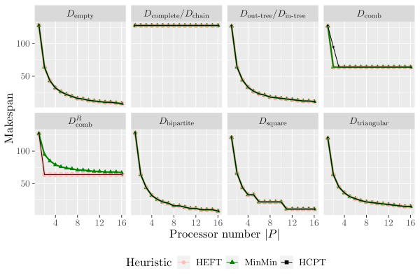
Figure 2: Makespan obtained with three heuristics (described in Section 6) on all special DAGs of Section 4 for $P|p_{j}=1,prec|C_{\max}$. The number of vertices is $n=128$ for the empty DAG, complete and bipartite DAGs, $n=127$ for the trees and combs, $n=121$ for the square DAG, and $n=120$ for the triangular DAG ($1+\cdots+15=120$).

Figure 2 shows the makespan obtained with three scheduling heuristics with all special DAGs as the number of processors varies. HEFT is always optimal because of the regularity of the DAG structures and because costs are unitary. This is also the case for the other heuristics most of the time. A zero mass, for long DAGs such as the complete DAG and chain, leads to an even easier scheduling problem where the number of processors has no impact. This confirms the discussion in Section 3.3 stating that low mass is characteristic of easy instances. For the other DAGs, increasing the number of processors decreases the makespan until it reaches 1, 2, 7, 11, 15 and 50 for the empty DAG, bipartite DAG, trees, square DAG, triangular DAG and combs, respectively. Note that the stairs for the square are due to its layered structure. For the reversed comb, MinMin behaves poorly because this simple heuristic does not take into account the critical path and fill the processors with any of the initial source vertices. Finally, the sub-optimal schedule produced by HCPT for the comb DAG is because, contrarily to HEFT with its insertion mechanism, this heuristic does not rely on backfilling and cannot schedule a task before any other already scheduled tasks.

5 Analysis of Existing Generation Methods

This section covers and analyzes existing generation methods: the classic Erdős-Rényi algorithm; a uniform random generation method via a recursive approach; a poset-based method; and, an ad-hoc method frequently used in the scheduling literature.

5.1 Random Generation of Triangular Matrices

This approach is based on the Erdős-Rényi algorithm[ER59] with parameter $p$ (noted $G(n,p)$ in[Bol01]): an upper-triangular adjacency matrix is randomly generated. For each pair of vertices $(i,j)$, with $i<j$, there is an edge from $i$ to $j$ with an independent probability $p$. The expected number of edges is therefore $p\frac{n(n-1)}{2}$.

The approach is not uniform (nor uniform up to isomorphism). For instance, a generator that is uniform up to isomorphism picks up the empty DAG with probability $1/6$ (see Table 3). Moreover, a random generator that is uniform over all the DAGs (see Section 3.4 for the distinction) generates the empty DAG with probability $1/25$. With $p=0.5$, the Erdős-Rényi algorithm generates the DAG with no edges with probability $1/8$.

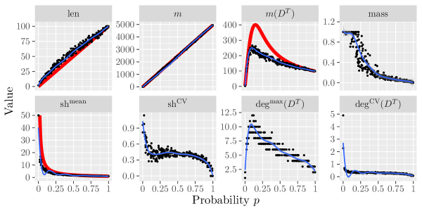
Figure 3: Properties of 300 DAGs of size $n=100$ generated by the Erdős-Rényi algorithm with probability $p$ uniformly drawn between 0 and 1. The smoothed line is obtained with a linear regression using a polynomial spline with 10 degrees of freedom. The degree CV (Coefficient of Variation) is the ratio of the mean degree to the degree standard deviation. Red lines correspond to formal results for the length and mean shape (Proposition 3), the number of edges, and the number of edges in the transitive reduction (Proposition 4).

Figures 3 and 4 show the effect of both parameters, probability $p$ and size $n$, on the properties of the generated DAGs. For readability of both figures, each standard deviation is replaced by a CV (Coefficient of Variation), which is the ratio of the standard deviation to the mean. The most evident effect on both figures is that the number of edges $m$ increases linearly as $p$ increases and quadratically as $n$ increases, which is a direct consequence of the algorithm and the expected number of edges. Similarly, but with more variation, the length also increases as either parameter increases. This effect also concerns the mean shape because $\textnormal{sh}^{\textnormal{mean}}=\frac{n}{\textnormal{len}}$ (for instance, the length is close to 20 when $p=0.125$, whereas the mean shape is close to 5). Therefore, on Figure 3, the mean shape decreases as the inverse function of the probability $p$ because the length increases quasi-linearly with $p$. This effect is consistent with Proposition 3 in Appendix B, which suggests that the expected mean shape is no greater than $\frac{1}{p}$.

A more remarkable effect can be seen for the number of edges in the transitive reduction $m(D^{T})$. This property shows that after a maximum around $p=0.10$, adding more edges with higher probabilities leads to redundant dependencies and simplifies the structure of the DAG by making it longer. The same observation can be done with $\textnormal{deg}_{\textnormal{}}^{\textnormal{max}}(D^{T})$. This is consistent with the fact that the algorithm generates the empty DAG when $p=0$ and the complete DAG when $p=1$. Proposition 4 in Appendix B also confirms this effect.

We rely on this apparent threshold around $p=10\%$ to characterize three probability intervals: below 5%, between 5% and 15%, and above 15%. DAGs generated with a probability in the first interval are almost empty (hence a length lower than 10 and a mean shape higher than 10) with few vertices having some edges and many with no edges (hence the high degree standard deviation). For these DAGs, most edges are not redundant. Given the high shape standard deviation, many tasks must be available at first. As mentioned in Section 3.2, these DAGs lead to a simplistic scheduling process that consists in starting each task on a critical path as soon as possible and then distributing a large number of independent tasks. Analogously, DAGs generated with probabilities $p$ greater than 15% contain many edges that simplify the DAG structure by increasing the length and thus reducing the mean shape (recall that with a small width, the problem is easy, see Section 3.2). At the same time, the mass decreases continuously, allowing the problem to be divided into smaller problems. In particular, for probability $p$ greater than 90%, DAGs are close to the chain, which is trivial to schedule. Therefore, most interesting DAGs are generated with probabilities between 5% and 15%.

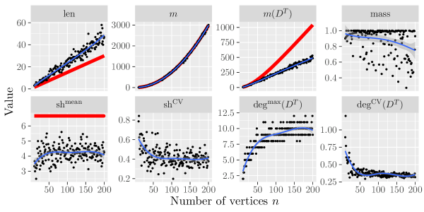
Figure 4: Properties of 191 DAGs generated by the Erdős-Rényi algorithm with probability $p=0.15$ and for each size $n$ between 10 and 200. The smoothed line is obtained with a linear regression using a polynomial spline with 4 degrees of freedom. Red lines correspond to formal results for the length and mean shape (Proposition 3), the number of edges, and the number of edges in the transitive reduction (Proposition 4).

As shown on Figure 4, the size of the DAG $n$ has a simpler effect on the number of edges in the transitive reduction $m(D^{T})$ than the probability $p$: $m(D^{T})$ increases linearly with $n$ (see Proposition 4). Moreover, the length increases with $n$ as the shape mean remains constant (see Proposition 3). As a consequence, the mass decreases with $n$ because the probability to obtain the value 1 increases in a vector with constant mean but increasing size. It is thus advisable to lower the probability with large sizes to maintain a constant mass.

The analysis of the Erdős-Rényi algorithm provides some insight on the desirable characteristics for the purpose of comparing scheduling heuristics. The effect of probability $p$ illustrates the compromise between the length and mean shape to avoid simplistic instances that are easily tackled (see Section 3.2). Moreover, the maximum number of edges in the transitive reduction $m(D^{T})$ is around $\frac{5}{2}n$ in both figures. However, we know that reaching $\frac{n^{2}}{4}$ is possible (Proposition 1) and layer-by-layer DAGs (square and triangular) are in $O(n^{\frac{3}{2}})$. Therefore, the Erdős-Rényi algorithm fails to generate DAGs with such large $m(D^{T})$.

5.2 Uniform Random Generation

There are two main ways to provide a uniform random generator to uniformly generate elements of $\mathcal{D}^{n}$ (uniform over all labelled DAGs, see Section 3.4). The first one consists in using a classical recursive/counting approach[Rob73]. This counting approach relies on recursively counting the number of DAGs with a given number of source vertices, that is vertices with no in-going edges. See[KM15, Section 4] for a complete algorithm that uniformly generates random DAGs with this approach. The second one relies on MCMC approaches[MDB01, IC02, MP04]. We describe below the recursive approach.

Let $a_{n}=|\mathcal{D}^{n}|$, $a_{n,s}$ be the number of DAGs of $\mathcal{D}^{n}$ having exactly $s$ source vertices ($\textnormal{sh}^{\textnormal{1}}=s$). It is proved in[Rob73] that:

$$a_{n}=\sum_{k=1}^{n}a_{n,k}\quad\text{and}\quad a_{n,k}={\binom{n}{k}}b_{n,k}\quad\text{with}\quad b_{n,k}=\sum_{s=1}^{n-k}(2^{k}-1)^{s}2^{k(n-k-s)}a_{n-k,s}.$$

First, we compute all values $a_{i}$ and $a_{i,k}$ for $1\leq i\leq n$ and $1\leq k\leq i$ with the initial conditions $a_{i,i}=1$ for $1\leq i\leq n$. Next, a shape is generated using Algorithm 1, where $\oplus$ is the concatenation of vectors.

1

Data: $n$, $a_{i}$, $a_{i,k}$ for $1\leq i\leq n$ and $1\leq k\leq i$.

Result: A shape with $n$ elements.

2

3Randomly generate $s\in\{1,n\}$ with distribution $\mathbb{P}(s=j)=\frac{a_{n,j}}{a_{n}}$;

4 return $[s]\oplus\textnormal{RandomShape}(n-s)$;

Algorithm 1 $\textnormal{RandomShape}(n)$

Finally, Algorithm 2 builds the final DAG by adding random edges.

1

Data: $[s_{1},\ldots,s_{k}]$ a shape with $n$ elements.

Result: A DAG with $n$ vertices.

2

3for $i\in[1,\ldots,k]$ do

4       for $j\in[1,\ldots,s_{i}]$ do

5             Generate a vertex $v$ with level $i$;

6             if $i>1$ then

7                   Connect a random vertex from level $i-1$ to vertex $v$;

8                   Connect any other vertex from previous levels to vertex $v$ with probability 0.5;

9                  

10             end if

11            

12       end for

13      

14 end for

15return the resulting DAG;

Algorithm 2 $\textnormal{ShapeToDAG}([s_{1},\ldots,s_{k}])$

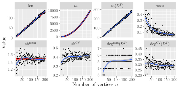
Figure 5: Properties of 191 DAGs generated by the recursive algorithm for each size $n$ between 10 and 200. The smoothed line is obtained with a linear regression using a polynomial spline with 4 degrees of freedom. Red lines correspond to formal results for the length and mean shape, and the number of edges (the bound from Theorem 2 is discarded because it is too far).

Figure 5 depicts the effect of the number of vertices on the selected DAG properties. Three effects are noteworthy: the length closely follows the function $\frac{3n}{2}$, the number of edges $m$ is almost indistinguishable from the function $\frac{n^{2}}{4}$ and the number of edges in the transitive reduction $m(D^{T})$ closely follows $1.4n$. The first effect is consistent with a theoretical result stating that the expected number of source vertices $\textnormal{sh}^{\textnormal{1}}$ in a uniform DAG is asymptotically 1.488 as $n\to\infty$[Lis75]. This implies that the expected value for each shape element is close to this value by construction of the shape. Proposition 7 in Appendix C confirms this expectation is no larger than 2.25, which makes the DAG an easy instance for scheduling problems (see Section 3.2). For the second effect, we know that the average number of edges in a uniform DAG is indeed $\frac{n^{2}}{4}$[MDB01, Theorem 2]. Despite the large amount of studies dedicated to formally analyzing uniform random DAGs, to the best of our knowledge, the last effect has not been formally considered. We finally observe that the mass decreases as the size $n$ increases. This is confirmed by the following result, proved in Appendix C:

Theorem 2.

Let $D$ be a DAG uniformly and randomly generated among the labeled DAGs with $n$ vertices. One has $\mathbb{P}(\textnormal{mass}^{\textnormal{abs}}(D)\geq\log^{4}(n))\to 0$ when $n\to+\infty$.

Therefore, the mass converges to zero as the size $n$ tends to infinity. As shown in Section 3.3, such instances can be decomposed into independent problems and efficiently solved with a brute force strategy. This leads to a sub-exponential generic time complexity with uniform instances.

To obtain a similar average number of edges $m$ with the Erdős-Rényi algorithm, we must choose a probability $p=0.5$. We can compare both methods by considering $p=0.5$ and $n=100$ on Figures 3 and 5, respectively. We observe that DAGs generated by both methods share similar properties. This leads to similar conclusions as in Section 5.1.

5.3 Random Orders

The random orders method derives a DAG from randomly generated orders[Win85]. The first step consists in building $K$ random permutations of $n$ vertices. Each of these permutations represents a total order on the vertices, which is also a complete DAG with a random labeling. Intersecting these complete DAGs by keeping an edge iff it appears in all DAGs with the same direction leads to the final DAG. This is a variant of the algorithm presented in[CMP⁺10] where the transitive reduction in the last step is not performed because we already measure the properties on the transitive reduction.

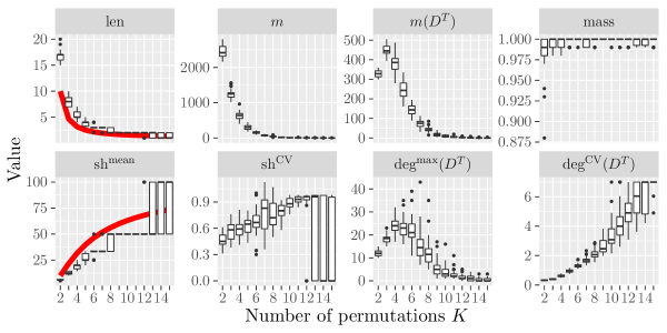
Figure 6: Properties of 420 DAGs of size $n=100$ generated by the random orders algorithm for each number of permutations $K$ between 2 and 15 (30 DAGs per boxplot). Red lines correspond to formal results for the length and mean shape.

Figure 6 shows the effect of the number of permutations $K$ on the DAG properties with boxplots. The extreme cases $K=1$ and $K\to\infty$ are discarded from the figure for clarity. They correspond to the chain and the empty DAG, respectively. Recall that for the chain, $m(D^{T})\approx\textnormal{len}=100$, $m\approx\numprint{5000}$, $\textnormal{sh}^{\textnormal{mean}}=\textnormal{deg}_{\textnormal{}}^{\textnormal{max}}(D^{T})=1$ and the CVs and mass are zero. Similarly, for the empty DAG, $\textnormal{len}=\textnormal{mass}=1$, the mean shape is 100 and all the other properties are zero.

The number of permutations quickly constrains the length. For instance, the length is already between 15 and 20 when $K=2$ and at most 5 when $K\geq 5$. A formal analysis suggests that the length is almost surely in $O(n^{1/K})$[Win85, Theorem 3], which is consistent with our observation. The number of edges and the maximum degree in the transitive reduction reach larger values than with previous approaches for any size $n$ (twice larger than with the Erdős-Rényi algorithm). Moreover, the mass is always close to one for $K>1$. Some specific values can finally be explained. First, the maximum value for $\textnormal{deg}_{\textnormal{}}^{\textnormal{CV}}(D^{T})$ is exactly 7 and corresponds to DAGs of size $n=100$ with a single edge (2 vertices have degree 1 and 98 others have 0). Also, the shape CV is at most 0.98 when the length is 2 (which frequently when $K\geq 10$). This CV corresponds to a shape with values 99 and 1.

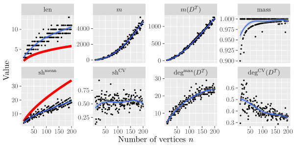
Figure 7: Properties of 191 DAGs generated by the random orders algorithm with $K=3$ permutations and for each size $n$ between 10 and 200. The smoothed line is obtained with a linear regression using a polynomial spline with 4 degrees of freedom. Red lines correspond to formal results for the length and mean shape.

Figure 7 shows the effect of the number of vertices $n$ for a fixed number of permutations $K$. We selected $K=3$ to have the maximum number of edges in the transitive reduction. The sublinear relation between the length and size $n$ is again consistent with the previously cited result (i.e. $O(n^{1/K})$). Even though $K=3$ is small, the length is already low, leading to line patterns for both the length and the mean shape. Note that the mass is frequently either 1 or almost 1 (i.e., $1-\frac{1}{k}$), which corresponds to cases where only the last value of the shape $\textnormal{sh}^{\textnormal{k}}$ is one.

The random orders method can generate denser DAGs than Erdős-Rényi or uniform DAGs without the mass issue, but with difficult control over the compromise between the length and the mean shape.

5.4 Layer-by-Layer

Many variants of the layer-by-layer principle have been used throughout the literature to assess scheduling algorithms and are covered in Section 2.4. This section analyzes the effect of three parameters (size $n$, number of layers $k$ and connectivity probability $p$) using the following variant inspired from[CMP⁺10, GCJ17]. First, $k$ vertices are affected to distinct layers to prevent any empty layer. Then, the remaining $n-k$ vertices are distributed to the layers using a balls into bins approach (i.e. a uniformly random layer is selected for each vertex). For each vertex not in the first layer, a random parent is selected among the vertices from the previous layer to ensure that the layer of any vertex equals its depth (similar to[DNSC09, GCJ17] and the recursive method in Section 5.2). Finally, random edges are added by connecting any pair of vertices from distinct layers from top to bottom with probability $p$.

This variant departs from[CMP⁺10, GCJ17] to ensure generated DAGs have a length equal to $k$ and mean shape equal to $n/k$. Moreover, with some parameter values, this method produces some of the special DAGs covered in Section 4. It generates the empty DAG when $k=1$, whereas it generates the complete DAG with $k=n$ and $p=1$. To interpret the number of edges depicted in Figures 8 to 10, we study the case (called regular) when all layers have the same size $n/k$, which constitutes an approximation of the DAGs generated by the layer-by-layer variant studied in this section. When $p=1$, the DAG is the bipartite one for $k=2$ and the square one for $k=\sqrt{n}$. In such DAGs and when $n$ is a multiple of $k$, the expected number of edges is

$$\mathbb{E}(m)=n\left(1-\frac{1}{k}\right)\left(p\left(\frac{n}{2}-1\right)+1\right)$$ (1)

and the expected number of edges in the transitive reduction is

$$\mathbb{E}(m(D^{T}))\geq p(k-1)\left(\frac{n}{k}\right)^{2}+(1-p)n\left(1-\frac{1}{k}\right).$$ (2)

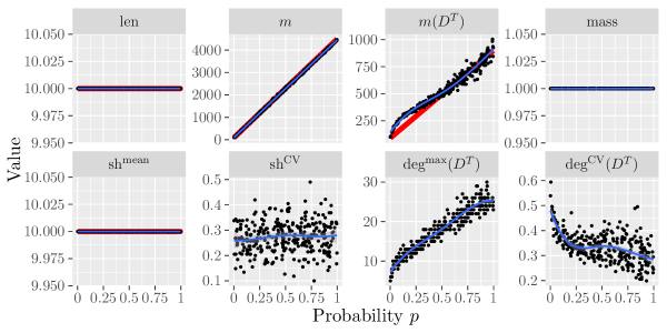
Figure 8: Properties of 300 DAGs of size $n=100$ generated by the layer-by-layer algorithm with $k=10$ layers and probability $p$ uniformly drawn between 0 and 1. The smoothed line is obtained with a linear regression using a polynomial spline with 4 degrees of freedom. Red lines correspond to formal results for the length and mean shape, the number of edges (Equation 1), the number of edges in the transitive reduction (Equation 2), and the mass.

Figure 8 shows the effect of the probability $p$. The analysis for regular layer-by-layer DAGs closely approximates the results. The number of edges $m$ is predicted to increase linearly from 90 to 4 500 (Equation 1), while this quantity in the transitive reduction $m(D^{T})$ is expected to increase from 90 to 900 (Equation 2). Remark that this last property undergoes a steeper increase for probability $p<0.1$ than for larger $p$. With many edges ($p>0.1$), adding a new one is likely to result into the introduction of redundant edges, which is not the case for $p<0.1$. More generally, the layered structure ensures a steady increase of $m(D^{T})$ as the probability $p$ increases because any edge between two consecutive layers cannot become redundant through the insertion of any edge. The mass is always close to one because the probability to have a layer with one vertex is close to zero with $k=10$ layers.

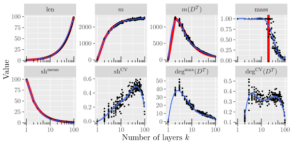
Figure 9: Properties of 300 DAGs of size $n=100$ generated by the layer-by-layer algorithm with probability $p=0.5$ and a number of layers $k$ randomly drawn between 1 and 100 ($k=\lfloor{e^{\mathcal{U}(\log(1),\log(101))}}\rfloor$ where $\mathcal{U}(a,b)$ is a uniform distribution between $a$ and $b$). The smoothed line is obtained with a linear regression using a polynomial spline with 5 degrees of freedom. Red lines correspond to formal results for the length and mean shape, the number of edges (Equation 1), the number of edges in the transitive reduction (Equation 2), and the mass.

Figure 9 represents the effect of the number of layers $k$. With regular layer-by-layer DAGs, the expected number of edges $\mathbb{E}(m)$ goes from 0 to 2 524,5 for $k=1$ to 100 (Equation 1), which is close to the results with our layer-by-layer variant. The increase is steep because it is already 2 295 for $k=10$, which is consistent with Figure 9. The number of edges in the transitive reduction $\mathbb{E}(m(D^{T}))$ decreases from an expected value of 1 275 to 99 as the number of layers goes from $k=2$ to 100 (Equation 2). The expected value for $k=10$ is 495 and is consistent with both Figures 8 and 9. Finally, the mass is unitary when there are at least two balls in each bin. Since there is initially one ball per bin, this occurs when there is at least one of the $n-k$ additional balls in each of the $k$ bin. To compute if there are enough additional balls to have a unitary mass with probability greater than $0.5$, we can use a bound for the coupon collector problem[LP17, Proposition 2.4]. This occurs when $\left\lceil k\log(2k)\right\rceil+k<n$, which is the case for $k\leq 20$ with $n=100$. This is consistent with Figure 9 where the mass becomes non-unitary around this value.

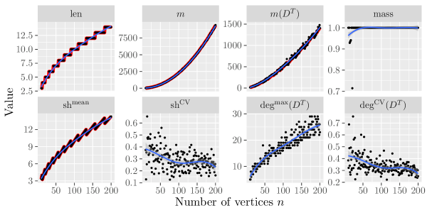
Figure 10: Properties of 191 DAGs generated by the layer-by-layer algorithm with probability $p=0.5$, $k=\sqrt{n}$ (rounded to closest integer) layers and for each size $n$ between 10 and 200. The smoothed line is obtained with a linear regression using a polynomial spline with 4 degrees of freedom. Red lines correspond to formal results for the length and mean shape, the number of edges (Equation 1), the number of edges in the transitive reduction (Equation 2), and the mass.

When varying the number of vertices $n$, we expect the number of edges $m$ to increase quadratically from 20 to around 9 380 (Equation 1), which is consistent with the results on Figure 10. Similarly, the number of edges in the transitive reduction $m(D^{T})$ is expected to increase quadratically from around 14.4 to around 1 420 (Equation 2).

In Figures 8 to 10, the length and mean shape show stable behavior consistent with our expectation. In all figures, the shape CV can formally be analyzed using the balls into bins model and we refer the interested reader to the specialized literature[KSC78]. Finally, in the transitive reduction, the maximum degree $\textnormal{deg}_{\textnormal{}}^{\textnormal{max}}(D^{T})$ has a similar trend as the number of edges $m(D^{T})$.

To avoid non-unitary mass, the layer-by-layer method can be adapted to ensure that each layer has two vertices initially. For instance, we can rely on a uniform distribution between two and a maximum value, or on a balls into bins approach with two balls per bin initially. It is also possible to use the method described in[CSH18, Section III] to have a uniform distribution of the vertices in the layers over all possible distributions and with a constraint on the minimum value.

6 Evaluation on Scheduling Algorithms

Generating random task graphs allows the assessment of existing scheduling algorithms in different contexts. Numerous heuristics have been proposed for the problem denoted $P|p_{j}=1,prec|C_{\max}$ (homogeneous tasks and processors, see Section 3.2) or generalization of this problem. Such heuristics rely on different principles. Some simple strategies, like MinMin, execute available tasks on the processors that minimize completion time without considering precedence constraints. In contrast, many heuristics sort tasks by criticality and schedule them with the Earliest Finish Time (EFT) policy (e.g. HEFT and HCPT). Finally, other principles may be also used: migration for BSA[KA00], clustering for DSC[YG94], etc. We focus on the impact of generation methods on the performance of a selection of three heuristics for this problem: MinMin, HEFT and HCPT.

HEFT[THW02] (Heterogeneous Earliest Finish Time) first computes the upward rank of each task, which can be seen as a reversal depth (depth in the reversal DAG). It then consider tasks by decreasing order of their upward ranks and schedules them with the EFT policy. Backfilling is performed following an insertion policy that tries to insert a task at the earliest idle time between two already scheduled tasks on a processor if the slot is large enough to accommodate it. The time complexity of this approach is dominated by the insertion policy in $O(n^{2})$. Numerous heuristics are equivalent to HEFT when tasks and processors are homogeneous: PEFT[AB14], HLEFT[ACD74], HBMCT[SZ04].

HCPT[HJ03] (Heterogeneous Critical Parent Trees) starts by considering any task on a critical path by decreasing order of their depth. The objective is to prioritize the ancestors of such tasks and in particular when their depth is large. This process generates a priority list of tasks that are then scheduling with the EFT policy. The time complexity is $O(m+n\log(n)+n|P|)$ where $|P|$ is the number of processors.

Finally, MinMin[IK77, Algorithm D][FGA⁺98, minmin] considers all available tasks any time a processor becomes idle and schedules any task on any available processor. With homogeneous tasks and processors, this algorithm is equivalent to MaxMin[IK77, Algorithm E][FGA⁺98, maxmin]. The time complexity is $O(m)$.

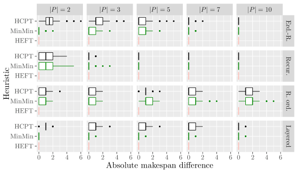
Figure 11: Difference between the makespan obtained with any heuristic and the best value among the three heuristics for each instance. Each boxplot represents the results for 300 DAGs of size $n=100$ built with one of the following methods: the Erdős-Rényi algorithm with probability $p=0.15$, the recursive algorithm, the random orders algorithm with $K=3$ permutations and the layer-by-layer algorithm with probability $p=0.5$ and a number of layers $k=10$. Costs are unitary and $|P|$ represents the number of processors.

Figure 11 shows the absolute difference between HEFT, HCPT and MinMin for each generation method covered in Section 5. Despite guaranteeing an unbiased generation, instances built with the recursive algorithm fail to discriminate heuristics except when there are two processors. Recall that the mean shape is close to $1.5$ for such DAGs and few processors are sufficient to obtain a makespan equal to the DAG length (i.e. an optimal schedule). In contrast, instances built with the random orders algorithm lead to difference performance for each scheduling heuristics. However, this generation method has no uniformity guarantee and its discrete parameter $K$ limits the diversity of generated DAGs. Finally, the last two algorithms, Erdős-Rényi and layer-by-layer, fail to highlight a significant difference between MinMin and HEFT even though the former scheduling heuristic can be expected to be inferior to the latter because it discards the DAG structure.

To support these observations, we analyse below the maximum difference between the makespan obtained with HEFT and the ones obtained with the other two heuristics. Because it lacks any backfilling mechanism, HCPT performs worse than HEFT with an instance composed of the following two elements. First, a chain of length $k$ with $|P|-1$ additional tasks with predecessor the $(k-2)$th task of the chain and successor the $k$th task of the chain. Alternatively, this first element can be seen as a chain of length $k-3$ connected to a fork-join with width $|P|$. The second element is a chain of length $k-1$. HCPT schedules the first element and then the second one afterward, leading to a makespan of $2k-1$ whereas the optimal one is $k$. With $n=100$ tasks and $|P|\leq 10$, the difference from HEFT with this instance is greater than or equal to 45. Moreover, MinMin also performs worse with specific instances. Consider the ad hoc instances considered in[CMSV18] each consisting of one chain of length $k$ and a set of $k(|P|-1)$ independent tasks. Discarding the information about critical tasks prevents MinMin from prioritizing tasks from the chain. With $n=100$ tasks and with $|P|\leq 10$, the worst-case absolute difference can be greater than or equal to 9 (when MinMin completes first the independent before starting the chain). While the difficult instances for HCPT rely on a specific weakness, it is interesting to analyse the properties of the difficult instances for MinMin. Each DAG is characterized by a length equal to $\textnormal{len}=\frac{n}{|P|}$ and a number of edges in the transitive reduction $m(D^{T})=\textnormal{len}-1$ (leading to a large width and a large shape standard deviation). With $n=100$ tasks, with both HCPT and MinMin, the absolute difference from HEFT can be greater than or equal to 9.

Theses experiments illustrate the need for better generation methods that control multiple properties while avoiding any generation bias. An ideal generation method would uniformly select a DAG over all existing DAGs having a given number of tasks $n$, number of edges $m$ and/or $m(D^{T})$, length and/or width, and with a unitary mass.

7 Conclusion

This work contributes in three ways to the final objective of uniformly generating random DAGs belonging to a category of instances with desirable characteristics. First, we identify a list of 34 DAG properties and focus on a selection of 8 such properties. Among these, the mass quantifies how much an instance can be decomposed into smaller ones. Second, existing random generation methods are formally analyzed and empirically assessed with respect to the selected properties. Establishing the sub-exponential generic time complexity for decomposable scheduling problems with uniform instances constitutes the most noteworthy result of this paper. Last, we study how the generation methods impact scheduling heuristics with unitary costs.

The relevance and impact of many other properties need to be investigated. For instance, the number of tasks present on a critical path can exceed the length and even reach $n$. Also, we could measure the distance of a DAG from a serie-parallel one by counting with the minimum number of edges to remove in the former DAG to obtain the latter one. Both these measures may impact the performance of scheduling heuristics.

Adapting current results to instances with communication costs requires some adaptations that need to be explored. For instance, each edge with a cost could be discarded when there is another path of higher processing cost (i.e. assuming all communication costs are null on this path). The definition of the mass could state that a vertex is a bottleneck vertex when no edge connect a preceding vertex to a following one.

Finally, extending properties to instances with non-unitary costs is left to future work. For instance, the shape could be replaced by the continuous occupation of the DAG when scheduled on an infinite number of processors (i.e. the number of occupied processors at each time step). As a result, the length would be the critical path length and the mean shape would be the sum of all costs (called the work) divided by the critical path length (called parallelism in[TK02]).

Appendix A Exact Properties of Special DAGs

Tables 6 and 7 synthesize the exact properties of the special DAGs presented in Section 4.

DAG	$m$	$\textnormal{deg}_{\textnormal{}}^{\textnormal{max}}$	$\textnormal{deg}_{\textnormal{in}}^{\textnormal{max}}$	$\textnormal{deg}_{\textnormal{out}}^{\textnormal{max}}$	$\textnormal{deg}_{\textnormal{}}^{\textnormal{min}}$	$\textnormal{deg}_{\textnormal{}}^{\textnormal{mean}}$	$\textnormal{deg}_{\textnormal{}}^{\textnormal{sd}}$	$\textnormal{deg}_{\textnormal{in}}^{\textnormal{sd}}$	$\textnormal{deg}_{\textnormal{out}}^{\textnormal{sd}}$
$D_{\textnormal{empty}}$	0	0	0	0	0	0	0	0	0
$D_{\textnormal{complete}}$	$\frac{n(n-1)}{2}$	$n-1$	$n-1$	$n-1$	$n-1$	$n-1$	0	$\sqrt{\frac{n^{2}-1}{12}}$	$\sqrt{\frac{n^{2}-1}{12}}$
$D_{\textnormal{chain}}$	$n-1$	$2$	$1$	$1$	$1$	$2(1-\frac{1}{n})$	$\sqrt{\frac{2}{n}(1-\frac{2}{n})}$	$\sqrt{\frac{1}{n}(1-\frac{1}{n})}$	$\sqrt{\frac{1}{n}(1-\frac{1}{n})}$
$D_{\textnormal{out-tree}}$ $D_{\textnormal{comb}}$	$n-1$	$3$	$1$	$2$	$1$	$2(1-\frac{1}{n})$	$\sqrt{1-\frac{1}{n}-\frac{4}{n^{2}}}$	$\sqrt{\frac{1}{n}(1-\frac{1}{n})}$	$\frac{\sqrt{n-1}\sqrt{n+1}}{n}$
$D_{\textnormal{in-tree}}$ $D_{\textnormal{comb}}^{R}$	$n-1$	$3$	$2$	$1$	$1$	$2(1-\frac{1}{n})$	$\sqrt{1-\frac{1}{n}-\frac{4}{n^{2}}}$	$\frac{\sqrt{n-1}\sqrt{n+1}}{n}$	$\sqrt{\frac{1}{n}(1-\frac{1}{n})}$
$D_{\textnormal{bipartite}}$	$\frac{n^{2}}{4}$	$\frac{n}{2}$	$\frac{n}{2}$	$\frac{n}{2}$	$\frac{n}{2}$	$\frac{n}{2}$	0	$\frac{n}{4}$	$\frac{n}{4}$
$D_{\textnormal{square}}$	$n(\sqrt{n}-1)$	$2\sqrt{n}$	$\sqrt{n}$	$\sqrt{n}$	$\sqrt{n}$	$2(\sqrt{n}-1)$	$\sqrt{2\sqrt{n}-4}$	$\sqrt{\sqrt{n}-1}$	$\sqrt{\sqrt{n}-1}$
$D_{\textnormal{triangular}}$	$\frac{k(k+1)(k-1)}{3}$	$2(k-1)$	$k-1$	$k$	2	$\frac{4}{3}(k-1)$	$\frac{\sqrt{2}}{3}(k-1)$	$\frac{\sqrt{(k-1)(k+2)}}{3\sqrt{2}}$	$\frac{\sqrt{(k-1)(k+14)}}{3\sqrt{2}}$

Table 6: Edge-related properties of special DAGs. For $D_{\textnormal{triangular}}$, $k$ is the length of the DAG ($k\approx\sqrt{2n}-\frac{1}{2}$ because $n=\frac{k(k+1)}{2}$).

DAG	len	$0pt$	$\textnormal{sh}^{\textnormal{max}}$	$\textnormal{sh}^{\textnormal{min}}$	$\textnormal{sh}^{\textnormal{mean}}$	$\textnormal{sh}^{\textnormal{sd}}$	$\textnormal{sh}^{\textnormal{1}}$	$\textnormal{sh}^{\textnormal{k}}$	mass
$D_{\textnormal{empty}}$	1	$n$	$n$	$n$	$n$	0	$n$	$n$	1
$D_{\textnormal{complete}}$ $D_{\textnormal{chain}}$	$n$	1	1	1	1	0	1	1	0
$D_{\textnormal{out-tree}}$	$\log_{2}(n+1)$	$\frac{n+1}{2}$	$\frac{n+1}{2}$	1	$\frac{n}{\log_{2}(n+1)}$	$\sqrt{\frac{n}{\log_{2}(n+1)}\left(\frac{n+2}{3}-\frac{n}{\log_{2}(n+1)}\right)}$	1	$\frac{n+1}{2}$	$1-\frac{1}{n}$
$D_{\textnormal{in-tree}}$	$\log_{2}(n+1)$	$\frac{n+1}{2}$	$\frac{n+1}{2}$	1	$\frac{n}{\log_{2}(n+1)}$	$\sqrt{\frac{n}{\log_{2}(n+1)}\left(\frac{n+2}{3}-\frac{n}{\log_{2}(n+1)}\right)}$	$\frac{n+1}{2}$	1	$1-\frac{1}{n}$
$D_{\textnormal{comb}}$	$\frac{n+1}{2}$	$\frac{n+1}{2}$	2	1	$2(1-\frac{1}{n+1})$	$\sqrt{\frac{2}{n+1}(1-\frac{2}{n+1})}$	1	2	$1-\frac{1}{n}$
$D_{\textnormal{comb}}^{R}$	$\frac{n+1}{2}$	$\frac{n+1}{2}$	$\frac{n+1}{2}$	1	$2(1-\frac{1}{n+1})$	$\frac{n-1}{n+1}\sqrt{\frac{n-1}{2}}$	$\frac{n+1}{2}$	1	$\frac{1}{2}+{1}{2n}$
$D_{\textnormal{bipartite}}$	2	$\frac{n}{2}$	$\frac{n}{2}$	$\frac{n}{2}$	$\frac{n}{2}$	0	$\frac{n}{2}$	$\frac{n}{2}$	1
$D_{\textnormal{square}}$	$\sqrt{n}$	$\sqrt{n}$	$\sqrt{n}$	$\sqrt{n}$	$\sqrt{n}$	0	$\sqrt{n}$	$\sqrt{n}$	1
$D_{\textnormal{triangular}}$	$k$	$k$	$k$	1	$\frac{k+1}{2}$	$\sqrt{\frac{k^{2}-1}{12}}$	1	$k$	$1-\frac{1}{n}$

Table 7: Vertex-related properties of special DAGs. For $D_{\textnormal{triangular}}$, $k$ is the length of the DAG ($k\approx\sqrt{2n}-\frac{1}{2}$ because $n=\frac{k(k+1)}{2}$).

Appendix B Probabilistic Properties of Random Triangular Matrices

We investigate in this section some probabilistic results on DAG generated by the Erdős-Rényi approach.

Proposition 3.

Let $D$ be a DAG with $n$ vertices randomly generated by the Erdős-Rényi algorithm with parameter $p$. Denoting by $(X_{1},\ldots,X_{k})$ its shape decomposition, one has, for each $1\leq i\leq k$, $\mathbb{E}(|X_{i}|)\leq\frac{1}{p}$.

Proof.

Let $M_{i,j}$ be the upper triangular matrix corresponding to $D$. Let $Y_{i}=\cup_{j<i}X_{j}$. If $j\in X_{i}$, then, for all $r<j$ such that $r\notin Y_{i}$, $M_{r,j}=0$. Therefore, since the $M_{r,j}$ are independent Bernoulli random variables of parameter $p$, $\mathbb{P}(j\in X_{i})\leq(1-p)^{j-|Y_{i}|}$. Consequently, $\mathbb{E}(x_{i})\leq 1+(1-p)+\ldots+(1-p)^{n-|Y_{i}|}\leq\frac{1}{1-(1-p)}=\frac{1}{p}$. ∎

Proposition 4.

Let $D$ be a DAG with $n$ vertices randomly generated by the Erdős-Rényi Algorithm with parameter $p$. One has $\mathbb{E}(m(D^{T}))\leq\frac{n-1}{p}-\frac{1-p^{2}}{p^{3}}(1-(1-p^{2})^{n-1})$.

Proof.

Let $M_{i,j}$ be the upper triangular matrix corresponding to $D$.

$$A=\{(i,j)\mid 1\leq i<j\leq n,\ (i,j)\in E\text{ s.t. }\forall i<r<j,\ (i,r)\notin E\text{ or }(r,j)\notin E\},$$

where $E$ is the set of edges of $D$. By definition of $D^{T}$, if $(i,j)\in D^{T}$, then $(i,j)\in A$. Consequently,

$$|D^{T}|\leq|A|.$$ (3)

Moreover, for every $i<j$, $\mathbb{P}((i,j)\in A)=\mathbb{P}(M_{i,j}=1\text{ and }\forall i<r<j,\ M_{i,r}=0\text{ or }M_{r,j}=0)$. Since the $M_{i,j}$ are independent Bernoulli random variables,

$$\mathbb{P}((i,j)\in A) =\mathbb{P}(M_{i,j}=1)\Pi_{r=i+1}^{j-1}\mathbb{P}(M_{i,r}=0\text{ or }M_{r,j}=0)$$

$$=p\Pi_{r=i+1}^{j-1}(1-\mathbb{P}(M_{i,r}=1\text{ and }M_{r,j}=1))$$

$$=p\Pi_{r=i+1}^{j-1}(1-p^{2})=p(1-p^{2})^{j-i-1}.$$

Let $A_{i,j}$ be the Bernoulli random variable encoding that $(i,j)\in A$. One has $|A|=\sum_{i<j}A_{i,j}$. Consequently,

$$\mathbb{E}(|A|) =\sum_{j=2}^{n}\sum_{i=1}^{j-1}\mathbb{E}(A_{i,j})=\sum_{j=2}^{n}\sum_{i=1}^{j-1}p(1-p^{2})^{j-i-1}$$

$$=\sum_{j=2}^{n}\sum_{r=0}^{j-2}p(1-p^{2})^{r}\quad\text{with }r=j-i-1$$

$$=p\sum_{j=2}^{n}\frac{1-(1-p^{2})^{j-1}}{1-(1-p^{2})}$$

$$=\frac{1}{p}\sum_{j=2}^{n}(1-(1-p^{2})^{j-1})$$

$$=\frac{n-1}{p}-\frac{1}{p}\sum_{j=2}^{n}(1-p^{2})^{j-1}$$

$$=\frac{n-1}{p}-\frac{1-p^{2}}{p}\sum_{j=0}^{n-2}(1-p^{2})^{j}$$

$$=\frac{n-1}{p}-\frac{1-p^{2}}{p}\frac{1-(1-p^{2})^{n-1}}{1-(1-p^{2})}$$

$$=\frac{n-1}{p}-\frac{1-p^{2}}{p^{3}}(1-(1-p^{2})^{n-1}).$$

One can conclude using Equation (3). ∎

Appendix C Probabilistic Properties of Random Uniform DAGs

We are interested in this section in the probabilistic properties of the shape of a DAG $D$ randomly generated with the uniform distribution as exposed in Section 5.2. In this context, we consider a random shape $(x_{1},\ldots,x_{k})$ generated by Algorithm 1 (for a DAG with $n$ vertices). Note that the length $k$ of the shape is a random variable and that the $x_{i}$’s are dependent random variables. However, the distribution of $x_{i}$ only depends on the sum of the $x_{j}$’s, with $j<i$ (formally, $\mathbb{P}(x_{i}=r\mid x_{1},\ldots,x_{i}-1)=\mathbb{P}(x_{i}=r\mid s_{i})=\frac{a_{n-s_{i},k}}{a_{n-s_{i}}}$). Let $s_{1}=0$ and for $i\geq 1$, $s_{i}=\sum_{j<i}x_{j}$. The following result is proved in[Lis75, Proposition 3]: if $n-s_{i}\geq 2$ and $r\geq 2$,

$$\mathbb{P}(x_{i}\leq r\mid s_{i})\geq 1-\frac{n-s_{i}-r}{n-s_{i}+1}\frac{2}{(r+1)!\ 2^{\frac{r(r-1)}{2}}}.$$ (4)

It follows from Equation (4), for $r\geq 2$ and if $n-s_{i}\geq 2$,

$$\mathbb{P}(x_{i}>r\mid s_{i})\leq\frac{n-s_{i}-r}{n-s_{i}+1}\frac{2}{(r+1)!\ 2^{\frac{r(r-1)}{2}}}\leq\frac{2}{(r+1)!\ 2^{\frac{r(r-1)}{2}}}.$$

The above equation still holds if $n-s_{i}<2$ since the probability is null.

These upper bounds show that the probability of having large values in the shape is very small. For instance, the probability that $x_{i}\geq 9$ is less than $10^{-11}$.

Moreover, since for $r>2$, $(r+1)!\geq 2^{r+1}$, one has for every $r>2$,

$$\mathbb{P}(x_{i}>r\mid s_{i})\leq 2^{-\frac{r(r+1)}{2}}.$$ (5)

The following lemma will be useful.

Lemma 5.

One has, for every $r>2$, $n\geq 2$, $\mathbb{P}(\max(x_{i})>r)\leq n2^{-\frac{r(r+1)}{2}}$.

Proof.

Let $A_{i,r}$ denotes the event $x_{i}\leq r$. One has

$$\mathbb{P}(\max(x_{i})\leq r)=\mathbb{P}(\bigcap_{1\leq i\leq k}A_{i,r})$$

$$=\mathbb{P}(A_{1,r})\mathbb{P}(A_{2,r}\mid A_{1,r})\ldots\mathbb{P}(A_{i,r}\mid A_{1,r},A_{2,r},\ldots,A_{i-1,r})\ldots\mathbb{P}(A_{k,r}\mid A_{1,r},A_{2,r},\ldots,A_{k-1,r})$$

Using Equation (5) and Bernoulli’s inequality, it follows that $\mathbb{P}(\max(x_{i})\leq r)\geq(1-2^{-\frac{r(r+1)}{2}})^{k}\geq(1-2^{-\frac{r(r+1)}{2}})^{n}\geq 1-n2^{-\frac{r(r+1)}{2}}.$ Now, $\mathbb{P}(\max(x_{i})>r)=1-\mathbb{P}(\max(x_{i})\leq r)\leq n2^{-\frac{r(r+1)}{2}}$. ∎

We can now claim an upper bound for the expected value of $\textnormal{sh}^{\textnormal{max}}(D)=\max(x_{i})$.

Proposition 6.

One has $\mathbb{E}(\max(x_{i}))=O(\log n)$.

Proof.

Let $h=\left\lfloor\sqrt{6\log_{2}n}\right\rfloor+1$.

$$\mathbb{E}(\max(x_{i})) =\sum_{r=1}^{n}\mathbb{P}(\max(x_{i})=r).r$$

$$=\sum_{r=1}^{h}r\mathbb{P}(\max(x_{i})=r)\quad+\quad\sum_{r=h+1}^{n}r\mathbb{P}(\max(x_{i})=r)$$

$$\leq\sum_{r=1}^{h}h\mathbb{P}(\max(x_{i})=r)+\sum_{r=h+1}^{n}r\mathbb{P}(\max(x_{i})=r)$$

$$\leq h^{2}+\sum_{r=h+1}^{n}r\mathbb{P}(\max(x_{i})\geq r)$$

$$\leq h^{2}+\sum_{r=h+1}^{n}r\mathbb{P}(\max(x_{i}>r-1)$$

$$\leq h^{2}+\sum_{r=h+1}^{n}rn2^{-\frac{r(r-1)}{2}}$$

$$\leq h^{2}+n2^{-\frac{h(h+1)}{2}}\sum_{r=h+1}^{n}r$$

$$\leq 6\log_{2}n+n^{3}2^{-\frac{h(h+1)}{2}}$$

Since $r>3$ for $n\geq 2$, we can apply Lemma 5 to eliminate the probability in the second term. Note that $2^{-\frac{h(h+1)}{2}}\leq 2^{-\frac{h^{2}}{2}}\leq 2^{-3\log_{2}n}$. Since $n^{3}2^{-3\log_{2}n}=1$, we have $\mathbb{E}(\max(x_{i}))\leq 6\log_{2}n+1$, proving the result. ∎

It is proved in[Lis75] that $\mathbb{E}(x_{1})$ converges to a constant (approximately 1.488) when $n$ grows to infinity. One can easily obtain a bound for each level and each $n$.

Proposition 7.

One has, for every $n\geq 2$, every $1\leq i\leq k$, $\mathbb{E}(x_{i})\leq 2+\frac{1}{4}$.

Proof.

$$\mathbb{E}(x_{i}) =\sum_{r=1}^{n}j\mathbb{P}(x_{i}=r)=\mathbb{P}(x_{i}=1)+2\mathbb{P}(x_{i}=2)+\sum_{r=3}^{n}r\mathbb{P}(x_{i}=r)$$

Note that $\mathbb{P}(x_{i}=1)+\mathbb{P}(x_{i}=2)\leq 1$.

$$\mathbb{E}(x_{i}) \leq 2+\sum_{r=3}^{n}\frac{r}{2^{r(r+1)/2}}\leq 2+\sum_{r=3}^{n}\frac{1}{2^{r}}\frac{r}{2^{(r+1)/2}}$$

$$\leq 2+\sum_{r=3}^{n}\frac{1}{2^{r}}.$$

Since $r\geq 3$ for $n\geq 2$, we can apply Lemma 5 to eliminate the probability in the last term. Since $\sum_{r=1}^{n}\frac{1}{2^{r}}\leq 1$, $\mathbb{E}(x_{i})\leq 2+\frac{1}{4}$. ∎

Previous results confirm experimental results in Section 5.2 and show that the values of the shape are all quite small. In order to evaluate the mass of a random DAG, we will now investigate the lengths of the bloc. More precisely, let

$$\ell_{\max}=\max\{\ell\mid\exists i\text{ s. t. }(1-x_{i})(1-x_{i+1})\ldots(1-x_{i+\ell-1})\neq 0\},$$

the maximum length of a sequence of consecutive $x_{i}$ non equal to $1$.

It is proved in[Lis75, page 407] that there exists a constant $0<\alpha_{0}<2/3$ such that for all $n$, $\mathbb{P}(x_{i}=1\mid s_{i})\geq\alpha_{0}$ (the constant proposed in[Lis75] is $\frac{1}{96}$ but practical evaluation leads to claim that the probability to have only a single vertex in a level is greater than or equal to $1/3$).

Lemma 8.

For every $r>0$, $\mathbb{P}(\ell_{\max}\geq\ell)\leq n(1-\alpha_{0})^{\ell}$.

Proof.

One has

$$\mathbb{P}((1-x_{i}) (1-x_{i+1})\ldots(1-x_{i+\ell-1})\neq 0\mid s_{i})$$

$$=\mathbb{P}((1-x_{i})\neq 0\mid s_{i})\mathbb{P}((1-x_{i+1})\ldots(1-x_{i+\ell-1})\neq 0\mid s_{i}\text{ and }x_{1}\neq 1)$$

$$\leq(1-\alpha_{0})\mathbb{P}((1-x_{i+1})\ldots(1-x_{i+\ell-1})\neq 0\mid s_{i+1})$$

By a direct induction, one get $\mathbb{P}((1-x_{i})(1-x_{i+1})\ldots(1-x_{i+\ell-1})\neq 0\mid s_{i})\leq(1-\alpha_{0})^{\ell}$. Now let $\overline{x}_{i}$ be defined, for $1\leq i\leq n$ by $\overline{x}_{i}=x_{i}$ if $i\leq k$ and $\overline{x}_{i}=1$ otherwise. We also denote by $\overline{s}_{i}$ the sum $\sum_{j=1}^{-1}\overline{x}_{i}$.

$$\mathbb{P}(\ell_{\max}\geq\ell) =\mathbb{P}(\cup_{i=1}^{k-\ell+1}\{(1-x_{i})(1-x_{i+1})\ldots(1-x_{i+\ell-1})\neq 0\mid s_{i}\})$$

$$\leq\mathbb{P}(\cup_{i=1}^{n-\ell+1}\{(1-\overline{x}_{i})(1-\overline{x}_{i+1})\ldots(1-\overline{x}_{i+\ell-1})\neq 0\mid\overline{s}_{i}\})$$

$$\leq\sum_{i=1}^{k-n+1}\mathbb{P}((1-x_{i})(1-x_{i+1})\ldots(1-x_{i+\ell-1})\neq 0\mid s_{i})$$

$$\leq n(1-\alpha_{0})^{\ell},$$

proving the result. ∎

One can now prove Theorem 2.

Proof of Theorem 2.

Consider the event $A_{n}=\textnormal{sh}^{\textnormal{max}}(D)\geq\log^{2}(n)$ and $B_{n}=\ell_{\max}(D)\geq\log^{2}(n)$. Using Markov Inequality and Proposition 6, $\mathbb{P}(A_{n})\leq\frac{1}{\log n}$. Therefore, $\mathbb{P}(A_{n})\to 0$ when $n\to+\infty$.

Moreover $\mathbb{P}(B_{n})\leq n(1-\alpha_{0})^{\log^{2}n}$ by Lemma 8. But $\log(n(1-\alpha_{0})^{\log^{2}n})=\log n+\log(1-\alpha_{0})\log^{2}n$. Since $0<1-\alpha_{0}<1$, $\log n+\log(1-\alpha_{0})\log^{2}n\to-\infty$ when $n\to+\infty$. Consequently $n(1-\alpha_{0})^{\log^{2}n}\to 0$ when $n\to+\infty$.

Therefore $\mathbb{P}(A_{n}\cup B_{n})\to 0$ when $n\to+\infty$. ∎

References

- [AAK+13] Deepak Ajwani, Shoukat Ali, Kostas Katrinis, Cheng-Hong Li, Alfred J Park, John P Morrison, and Eugen Schenfeld. Generating synthetic task graphs for simulating stream computing systems. Journal of Parallel and Distributed Computing, 73(10):1362–1374, 2013.
- [AAP+16] Mishra Ashish, Sharma Aditya, Verma Pranet, Abhijit R Asati, and Raju Kota Solomon. A modular approach to random task graph generation. Indian Journal of Science and Technology, 9(8), 2016.
- [AB14] Hamid Arabnejad and Jorge G Barbosa. List scheduling algorithm for heterogeneous systems by an optimistic cost table. IEEE Transactions on Parallel and Distributed Systems, 25(3):682–694, 2014.
- [ACD74] Thomas L Adam, K. Mani Chandy, and JR Dickson. A comparison of list schedules for parallel processing systems. Communications of the ACM, 17(12):685–690, 1974.
- [AGU72] Alfred V. Aho, Michael R Garey, and Jeffrey D. Ullman. The transitive reduction of a directed graph. SIAM Journal on Computing, 1(2):131–137, 1972.
- [AK98] Ishfaq Ahmad and Yu-Kwong Kwok. On exploiting task duplication in parallel program scheduling. IEEE Transactions on Parallel & Distributed Systems, 9:872–892, 1998.
- [AKN05] Mona Aggarwal, Robert D Kent, and Alioune Ngom. Genetic algorithm based scheduler for computational grids. In High Performance Computing Systems and Applications, 2005. HPCS 2005. 19th International Symposium on, pages 209–215. IEEE, 2005.
- [AM11] DI George Amalarethinam and GJ Joyce Mary. DAGEN-A Tool To Generate Arbitrary Directed Acyclic Graphs Used For Multiprocessor Scheduling. International Journal of Research and Reviews in Computer Science, 2(3):782, 2011.
- [AVÁM92] Virgílio AF Almeida, IMM Vasconcelos, Jose Nagib Cotrim Árabe, and Daniel A Menascé. Using random task graphs to investigate the potential benefits of heterogeneity in parallel systems. In Proceedings of the 1992 ACM/IEEE conference on Supercomputing, pages 683–691. IEEE Computer Society Press, 1992.
- [BLDMK14] Bruno Bodin, Youen Lesparre, Jean-Marc Delosme, and Alix Munier-Kordon. Fast and efficient dataflow graph generation. In Proceedings of the 17th International Workshop on Software and Compilers for Embedded Systems, pages 40–49. ACM, 2014.
- [Bol01] Béla Bollobás. Random Graphs. Cambridge University Press, 2001.
- [CDB+16] Pedro Campos, Nizar Dahir, Colin Bonney, Martin Trefzer, Andy Tyrrell, and Gianluca Tempesti. Xl-stage: A cross-layer scalable tool for graph generation, evaluation and implementation. In Embedded Computer Systems: Architectures, Modeling and Simulation (SAMOS), 2016 International Conference on, pages 354–359. IEEE, 2016.
- [CLRS09] Thomas H Cormen, Charles E Leiserson, Ronald L Rivest, and Clifford Stein. Introduction to algorithms. MIT press, 2009.
- [CMP+10] Daniel Cordeiro, Grégory Mounié, Swann Perarnau, Denis Trystram, Jean-Marc Vincent, and Frédéric Wagner. Random graph generation for scheduling simulations. In Proceedings of the 3rd international ICST conference on simulation tools and techniques, page 60. ICST (Institute for Computer Sciences, Social-Informatics and Telecommunications Engineering), 2010.
- [CMRT88] Michel Cosnard, Mounir Marrakchi, Yves Robert, and Denis Trystram. Parallel gaussian elimination on an mimd computer. Parallel Computing, 6(3):275–296, 1988.
- [CMSV18] Louis-Claude Canon, Loris Marchal, Bertrand Simon, and Frédéric Vivien. Online scheduling of task graphs on hybrid platforms. In European Conference on Parallel Processing, pages 192–204. Springer, 2018.
- [CSH18] Louis-Claude Canon, Mohamad El Sayah, and Pierre-Cyrille Héam. A Markov Chain Monte Carlo Approach to Cost Matrix Generation for Scheduling Performance Evaluation. In International Conference on High Performance Computing & Simulation (HPCS), 2018.
- [CSH19] Louis-Claude Canon, Mohamad El Sayah, and Pierre-Cyrille Héam. Code to compare random task graph generation methods, February 2019. https://figshare.com/articles/Code_to_compare_random_task_graph_generation_methods/7725545/1.
- [DBGL+97] Giuseppe Di Battista, Ashim Garg, Giuseppe Liotta, Roberto Tamassia, Emanuele Tassinari, and Francesco Vargiu. An experimental comparison of four graph drawing algorithms. Computational Geometry, 7(5-6):303–325, 1997.
- [DNSC09] Pierre-Francois Dutot, Tchimou N’takpé, Frederic Suter, and Henri Casanova. Scheduling parallel task graphs on (almost) homogeneous multicluster platforms. IEEE Transactions on Parallel and Distributed Systems, 20(7):940–952, 2009.
- [DRW98] Robert P Dick, David L Rhodes, and Wayne Wolf. TGFF: task graphs for free. In Proceedings of the 6th international workshop on Hardware/software codesign, pages 97–101. IEEE Computer Society, 1998.
- [DŠTR12] Tatjana Davidović, Milica Šelmić, Dušan Teodorović, and Dušan Ramljak. Bee colony optimization for scheduling independent tasks to identical processors. Journal of heuristics, 18(4):549–569, 2012.
- [ER59] P Erdős and Alfréd Rényi. On random graphs I. Publ. Math. Debrecen, 6:290–297, 1959.
- [Fag76] Ronald Fagin. Probabilities on finite models. J. Symb. Log., 41(1):50–58, 1976.
- [FGA+98] Richard F Freund, Michael Gherrity, Stephen Ambrosius, Mark Campbell, Mike Halderman, Debra Hensgen, Elaine Keith, Taylor Kidd, Matt Kussow, John D Lima, Francesca Mirabile, Lantz Moore, Brad Rust, and Howard Jay Siegel. Scheduling resources in multi-user, heterogeneous, computing environments with SmartNet. In Heterogeneous Computing Workshop (HCW), pages 184–199. IEEE, 1998.
- [FJF16] Lester Randolph Ford Jr and Delbert Ray Fulkerson. Flows in networks. Princeton university press, 2016. First edition in 1962.
- [GCJ17] Indrajeet Gupta, Anubhav Choudhary, and Prasanta K Jana. Generation and proliferation of random directed acyclic graphs for workflow scheduling problem. In Proceedings of the 7th International Conference on Computer and Communication Technology, pages 123–127. ACM, 2017.
- [GJ78] M.R. Garey and D.S. Johnson. Strong NP-completeness results: motivation, examples, and implications. J. Assoc. Comput. Mach., 25(3):499–508, 1978.
- [GLLK79] R. L. Graham, E. L. Lawler, J. K. Lenstra, and A. H. G. Rinnooy Kan. Optimization and approximation in deterministic sequencing and scheduling: a survey. Annals of Discrete Mathematics, 5:287–326, 1979.
- [HJ03] Tarek Hagras and Jan Janecek. A simple scheduling heuristic for heterogeneous computing environments. In International Symposium on Parallel and Distributed Computing, page 104. IEEE, 2003.
- [IC02] Jaime Shinsuke Ide and Fábio Gagliardi Cozman. Random generation of bayesian networks. In Advances in Artificial Intelligence, 16th Brazilian Symposium on Artificial Intelligence, SBIA 2002, Porto de Galinhas/Recife, Brazil, November 11-14, 2002, Proceedings, Lecture Notes in Computer Science, pages 366–375, 2002.
- [IK77] Oscar H. Ibarra and Chul E. Kim. Heuristic Algorithms for Scheduling Independent Tasks on Nonidentical Processors. Journal of the ACM, 24(2):280–289, April 1977.
- [IT07] E Ilavarasan and P Thambidurai. Low complexity performance effective task scheduling algorithm for heterogeneous computing environments. Journal of Computer sciences, 3(2):94–103, 2007.
- [Jai90] Raj Jain. The art of computer systems performance analysis: techniques for experimental design, measurement, simulation, and modeling. John Wiley & Sons, 1990.
- [JCD+13] Gideon Juve, Ann Chervenak, Ewa Deelman, Shishir Bharathi, Gaurang Mehta, and Karan Vahi. Characterizing and profiling scientific workflows. Future Generation Computer Systems, 29(3):682–692, 2013.
- [KA99] Yu-Kwong Kwok and Ishfaq Ahmad. Benchmarking and comparison of the task graph scheduling algorithms. Journal of Parallel and Distributed Computing, 59(3):381–422, 1999.
- [KA00] Yu-Kwong Kwok and Ishfaq Ahmad. Link contention-constrained scheduling and mapping of tasks and messages to a network of heterogeneous processors. Cluster Computing, 3(2):113–124, 2000.
- [KM15] Jack Kuipers and Giusi Moffa. Uniform random generation of large acyclic digraphs. Statistics and Computing, 25(2):227–242, 2015.
- [KN09] Brian Karrer and Mark EJ Newman. Random graph models for directed acyclic networks. Physical Review E, 80(4):046110, 2009.
- [KSC78] Valentin Fedorovich Kolchin, Boris Aleksandrovich Sevastyanov, and Vladimir Pavlovich Chistyakov. Random allocations. Winston, 1978.
- [KSD95] Rainer Kolisch, Arno Sprecher, and Andreas Drexl. Characterization and generation of a general class of resource-constrained project scheduling problems. Management science, 41(10):1693–1703, 1995.
- [LALG13] Jing Li, Kunal Agrawal, Chenyang Lu, and Christopher Gill. Outstanding paper award: Analysis of global edf for parallel tasks. In Real-Time Systems (ECRTS), 2013 25th Euromicro Conference on, pages 3–13. IEEE, 2013.
- [Leu04] Joseph YT Leung. Handbook of scheduling: algorithms, models, and performance analysis. CRC Press, 2004.
- [Lis75] V.A. Liskovets. On the number of maximal vertices of a random acyclic digraph. Theory Probab. Appl., 20(2):401–409, 1975.
- [LKK83] R E_ Lord, JS Kowalik, and S_P Kumar. Solving linear algebraic equations on an mimd computer. Journal of the ACM (JACM), 30(1):103–117, 1983.
- [LP17] David A Levin and Yuval Peres. Markov chains and mixing times, volume 107. American Mathematical Society, 2017.
- [Man07] Willem Mantel. Problem 28. Wiskundige Opgaven, 10(60-61):320, 1907.
- [Mar18] Apolinar Velarde Martinez. Synthetic loads analysis of directed acyclic graphs for scheduling tasks. International Journal of Advanced Computer Science and Applications, 9(3):347–354, 2018.
- [MDB01] Guy Melançon, I. Dutour, and Mireille Bousquet-Mélou. Random generation of directed acyclic graphs. Electronic Notes in Discrete Mathematics, 10:202–207, 2001.
- [MKI+03] Ron Milo, Nadav Kashtan, Shalev Itzkovitz, Mark EJ Newman, and Uri Alon. On the uniform generation of random graphs with prescribed degree sequences. arXiv preprint cond-mat/0312028, 2003.
- [MP04] Guy Melançon and Fabrice Philippe. Generating connected acyclic digraphs uniformly at random. Inf. Process. Lett., 90(4):209–213, 2004.
- [OVRO+18] Julian Oppermann, Sebastian Vollbrecht, Melanie Reuter-Oppermann, Oliver Sinnen, and Andreas Koch. GeMS: a generator for modulo scheduling problems: work in progress. In Proceedings of the International Conference on Compilers, Architecture and Synthesis for Embedded Systems, page 7. IEEE Press, 2018.
- [Plo07] Anatoly D Plotnikov. Experimental algorithm for the maximum independent set problem. arXiv preprint arXiv:0706.3565, 2007.
- [Rob73] R. W. Robinson. Counting labeled acyclic digraphs. In F. Harray, editor, New Directions in the Theory of Graphs, pages 239–273, New York, 1973. Academic Press.
- [SAHR12] Rishad A Shafik, Bashir M Al-Hashimi, and Jeff S Reeve. System-level design optimization of reliable and low power multiprocessor system-on-chip. Microelectronics Reliability, 52(8):1735–1748, 2012.
- [SGB06] Sander Stuijk, Marc Geilen, and Twan Basten. SDF3: SDF for Free. In Application of Concurrency to System Design, 2006. ACSD 2006. Sixth International Conference on, pages 276–278. IEEE, 2006.
- [SMD11] Boonyarith Saovapakhiran, George Michailidis, and Michael Devetsikiotis. Aggregated-dag scheduling for job flow maximization in heterogeneous cloud computing. In Global Telecommunications Conference (GLOBECOM 2011), 2011 IEEE, pages 1–6. IEEE, 2011.
- [SZ04] Rizos Sakellariou and Henan Zhao. A hybrid heuristic for dag scheduling on heterogeneous systems. In Parallel and Distributed Processing Symposium, 2004. Proceedings. 18th International, page 111. IEEE, 2004.
- [THW02] Haluk Topcuoglu, Salim Hariri, and Min-you Wu. Performance-effective and low-complexity task scheduling for heterogeneous computing. IEEE transactions on parallel and distributed systems, 13(3):260–274, 2002.
- [TK02] Takao Tobita and Hironori Kasahara. A standard task graph set for fair evaluation of multiprocessor scheduling algorithms. Journal of Scheduling, 5(5):379–394, 2002.
- [Ull75] J.D. Ullman. NP-complete scheduling problems. J. Comput. System Sci., 10:384–393, 1975.
- [WG90] M-Y Wu and Daniel D Gajski. Hypertool: A programming aid for message-passing systems. IEEE transactions on parallel and distributed systems, 1(3):330–343, 1990.
- [Win85] Peter Winkler. Random orders. Order, 1(4):317–331, 1985.
- [YG94] Tao Yang and Apostolos Gerasoulis. DSC: Scheduling parallel tasks on an unbounded number of processors. IEEE Transactions on Parallel and Distributed Systems, 5(9):951–967, 1994.