Asymptotically exact data augmentation:
models, properties and algorithms

Abstract

Data augmentation, by the introduction of auxiliary variables, has become an ubiquitous technique to improve convergence properties, simplify the implementation or reduce the computational time of inference methods such as Markov chain Monte Carlo ones. Nonetheless, introducing appropriate auxiliary variables while preserving the initial target probability distribution and offering a computationally efficient inference cannot be conducted in a systematic way. To deal with such issues, this paper studies a unified framework, coined asymptotically exact data augmentation (AXDA), which encompasses both well-established and more recent approximate augmented models. In a broader perspective, this paper shows that AXDA models can benefit from interesting statistical properties and yield efficient inference algorithms. In non-asymptotic settings, the quality of the proposed approximation is assessed with several theoretical results. The latter are illustrated on standard statistical problems. Supplementary materials including computer code for this paper are available online.

Keywords: Approximation, auxiliary variables, divide-and-conquer, Bayesian inference, robustness.

1 Introduction

Starting at least from the 1960s with the seminal paper of Hartley (1958) on the expectation-maximization (EM) algorithm, introducing auxiliary variables has been a widely adopted strategy to derive iterative algorithms able to deal with possibly complicated inference problems. Indeed, either by coming from statistical physics (Swendsen and Wang 1987) or by the broad statistical community (Dempster et al. 1977), auxiliary (also called latent) variables have been used to improve (Duane et al. 1987; Edwards and Sokal 1988; Marnissi et al. 2018) and/or simplify (Tanner and Wong 1987; Doucet et al. 2002) inference methods, such as maximum likelihood (ML) estimation or simulation-based ones. Insightful reviews of these methods were conducted by Besag and Green (1993); van Dyk and Meng (2001); Tanner and Wong (2010). Among many others, slice sampling and half-quadratic (HQ) methods are archetypal instances of such auxiliary variable-based methods. These methods, by introducing auxiliary variables, appear to be an interesting alternative when sampling cannot be performed directly from a target distribution $\pi$. Nonetheless, the superiority of simulation-based algorithms based on data augmentation (DA) over classical Markov chain Monte Carlo (MCMC) methods without DA is not obvious as pointed out by Polson (1996); Damien et al. (1999). DA methods have been found to be slower than single-site update approaches in some cases (Hurn 1997) and some improvements have been derived to cope with these problems such as partial decoupling (Higdon 1998) or the introduction of a working parameter (Meng and van Dyk 1997). Moreover, DA techniques are often used on a case-by-case basis (Geman and Reynolds 1992; Albert and Chib 1993; Geman and Yang 1995; Polson et al. 2013) and could not be applied in general scenarios due to the absence of exact DA schemes yielding an efficient inference and low computation costs.

Similarly to approximate Bayesian computation (ABC) methods to circumvent intractable likelihoods (Beaumont et al. 2002; Sisson et al. 2018b), these limitations can be tackled by considering approximate DA schemes that become exact asymptotically. For instance, inspired from the variable splitting technique used in the alternating direction method of multipliers (ADMM) (Boyd et al. 2011), Vono et al. (2019) and Rendell et al. (2020) recently and independently proposed a novel and broad Bayesian inference framework that can circumvent limitations of exact DA approaches. By introducing a collection of instrumental (also called splitting) variables, the aforementioned authors considered the inference from an approximate probability distribution which can be simpler, more efficient and distributed over multiple computational workers (e.g., machines or kernels).

This paper aims at deeply investigating a broad framework coined asymptotically exact data augmentation (AXDA) which encompasses previously proposed special instances such as approximate models used in Vono et al. (2019); Rendell et al. (2020), among others. More precisely, Section 2 details how such models can be built in a quasi-systematic and simple way which is highly appreciable compared to the case-by-case search of computationally efficient DA schemes. In Section 3, we revisit some already-proposed special instances of AXDA models in order to show the potential benefits of AXDA on specific examples and to exhibit interesting properties which can be generally inherited by AXDA approaches. In Section 4, we assess quantitatively the bias of AXDA models with non-asymptotic theoretical results by considering Wasserstein and total variation distances. Then, Section 5 illustrates the previous theoretical results and the benefits of the proposed methodology on several statistical problems. In order to facilitate the use of AXDA, we eventually point out that the supplementary material involves a dedicated section (Section 5) presenting how such models can be instantiated to perform efficient inference through classical simulation-based, variational Bayes (VB), optimization or expectation-maximization (EM) methods. The proofs are also given in the supplementary material, see Section 1.

2 Asymptotically exact data augmentation

This section introduces AXDA schemes that aim to circumvent exact DA main issue: the art (van Dyk and Meng 2001) of finding the exact DA associated to a statistical model and its inference limitations. For sake of simplicity, with little abuse, we shall use the same notations for a probability distribution and its associated probability density function (pdf).

2.1 Motivations

In this paper, we are interested in performing the inference of a variable of interest $\boldsymbol{\theta}\in\Theta\subseteq\mathbb{R}^{d}$, where $\Theta$ is a closed convex set and $\mathrm{dim}(\Theta)=d$, by relying on a probability distribution with density $\pi$ writing

$$\pi(\boldsymbol{\theta})\propto\exp\left(-f(\boldsymbol{\theta})\right),\quad\text{or}\quad\pi(\mathbf{y}|\boldsymbol{\theta})\propto\exp\left(-f(y;\boldsymbol{\theta})\right),$$ (1)

where the potential $f$ taking values in $\mathbb{R}$ is such that $\pi$ defines a proper, bounded and continuous probability distribution. For sake of generality, note that $\pi$ in (1) shall describe various quantities. First, with a little abuse of notations, $\pi(\boldsymbol{\theta})$ may simply refer to a pdf associated to the random variable $\boldsymbol{\theta}$, e.g., its prior distribution $\pi(\boldsymbol{\theta})$ or its posterior distribution $\pi(\boldsymbol{\theta})\triangleq\pi(\boldsymbol{\theta}|\mathbf{y})$ when referring to a set of observations denoted by $\mathbf{y}$. Depending on the problem, we also allow $\pi$ to stand for a likelihood function $\pi(\mathbf{y}|\boldsymbol{\theta})$. We will work under this convention and write explicitly the form of $\pi$ when required. For sake of simplicity and clarity, only the case corresponding to $\pi(\boldsymbol{\theta})$ will be detailed in this section. The application of the proposed methodology to $\pi(\mathbf{y}|\boldsymbol{\theta})$ is very similar and can be retrieved by a straightforward derivation.

We consider situations where direct inference from (1) is difficult because intractable or computationally prohibitive. To overcome these issues, an option is to rely on exact DA which introduces some auxiliary variables stacked into a vector $\mathbf{z}\in\mathcal{Z}\subseteq\mathbb{R}^{k}$ and defines a new density, simpler to handle, such that

$$\int_{\mathcal{Z}}\pi(\boldsymbol{\theta},\mathbf{z})\mathrm{d}\mathbf{z}=\pi(\boldsymbol{\theta}).$$ (2)

Much research has been devoted to these models in order to simplify an inference task or to improve the convergence properties of direct inference approaches (e.g., slice sampling and HQ methods introduced in Section 1). Nonetheless, these approaches have several limitations. Indeed, finding a convenient form for the augmented density in order to satisfy (2) while leading to efficient algorithms generally requires some knowledge and can even be impossible in some cases (Geman and Yang 1995). For instance, the mixture representation of a binomial likelihood function based on the Polya-Gamma distribution has been used to derive a promising Gibbs sampler for logistic regression problems (Polson et al. 2013). Nonetheless, even if this algorithm has been proved to be uniformly ergodic by Choi and Hobert (2013), the corresponding ergodicity constant depends exponentially on the number of observations $n$ and on the dimension of the regression coefficients vector $d$.

To tackle these limitations, we propose to relax the constraint (2) and consider an approximate DA model. This will permit the choice of an augmented density with more flexibility, fix the issues associated to the initial model and make inference more efficient in some cases. To this purpose, Section 2.2 presents the so-called AXDA framework which embeds approximate DA models controlled by a positive scalar parameter $\rho$. These models become asymptotically exact when $\rho$ tends towards 0. Of course, some assumptions will be required on the approximate augmented density to guarantee a good approximation. The quality of this approximation will be assessed in Section 4 with non-asymptotic theoretical results.

2.2 Model

Instead of searching for an exact data augmentation scheme (2), some auxiliary variables $\mathbf{z}$ can be introduced in order to define an approximate but asymptotically exact probability distribution. One possibility is to introduce an augmented distribution depending on a parameter $\rho>0$ and such that the associated marginal density defined by

$$\pi_{\rho}(\boldsymbol{\theta})=\int_{\mathcal{Z}}\pi_{\rho}(\boldsymbol{\theta},\mathbf{z})\mathrm{d}\mathbf{z},$$ (3)

satisfies the following property.

Property 1.

For all $\boldsymbol{\theta}\in\Theta$, $\lim_{\rho\rightarrow 0}\pi_{\rho}(\boldsymbol{\theta})=\pi(\boldsymbol{\theta})$ .

By applying Scheffé’s lemma (Scheffé 1947), this property yields the convergence in total variation, that is $\left\|\pi_{\rho}-\pi\right\|_{\mathrm{TV}}\rightarrow 0$ as $\rho\rightarrow 0$. A natural question is: how to choose the augmented density in (3) such that Property 1 is met? In this paper, we assume that $\mathcal{Z}=\Theta$ and investigate AXDA schemes associated to an initial density (1) and defined by the approximate augmented density

$$\pi_{\rho}(\boldsymbol{\theta},\mathbf{z})=\pi(\mathbf{z})\kappa_{\rho}(\mathbf{z},\boldsymbol{\theta}),$$ (4)

where $\kappa_{\rho}$ is such that (4) defines a proper density.

Remark 1.

When $\pi$ stands for a product of $J$ densities, that is $\pi\propto\prod_{j=1}^{J}\pi_{j}$, the proposed approximate model can naturally be generalized to $\pi_{\rho}(\boldsymbol{\theta},\mathbf{z}_{1\mathrel{\mathop{\mathchar 58\relax}}J})\propto\prod_{j=1}^{J}\pi_{j}(\mathbf{z}_{j})\kappa_{\rho}(\mathbf{z}_{j},\boldsymbol{\theta})$. Such a generalization will for instance be considered in Sections 3.1 and 3.2.

The introduction of the proposed model (4) is aimed at avoiding a case-by-case search of an appropriate augmented approach. Although there might exist other marginal densities $\pi_{\rho}$ satisfying Property 1, we restrict our analysis to models where $\kappa_{\rho}(\cdot,\boldsymbol{\theta})$ weakly converges towards the Dirac measure at $\boldsymbol{\theta}$ as $\rho\rightarrow 0$ (Aguirregabiria et al. 2002). This is a sufficient condition to satisfy Property 1. In the sequel, we will call AXDA any approach based on (4) and satisfying these properties.

A natural choice for $\kappa_{\rho}$ is to consider a standard kernel $K$ (Wand and Jones 1995). Based on the latter, we define for all $\mathbf{z},\boldsymbol{\theta}\in\Theta$, $\kappa_{\rho}(\mathbf{z},\boldsymbol{\theta})\propto_{\mathbf{z}}\rho^{-d}K(\rho^{-1}(\boldsymbol{\theta}-\mathbf{z}))$ (Dang and Ehrhardt 2012). Beyond standard kernels but motivated by the same idea of measuring the discrepancy between $\mathbf{z}$ and $\boldsymbol{\theta}$, one can also build on divergence functions widely used in the optimization literature to define a potentially asymmetric density $\kappa_{\rho}$ such that for all $\mathbf{z},\boldsymbol{\theta}\in\Theta$, $\kappa_{\rho}(\mathbf{z},\boldsymbol{\theta})\propto_{\mathbf{z}}\exp(-\rho^{-1}\phi(\mathbf{z},\boldsymbol{\theta}))$ where $\phi$ is a strictly convex function w.r.t. $\mathbf{z}$ admitting a unique minimizer $\mathbf{z}^{*}=\boldsymbol{\theta}$ (Ben-Tal et al. 2001; Krichene et al. 2015; Fellows et al. 2019). Specific instances of such potentials are Bregman divergences such as the logistic loss and the Kullback-Leibler divergence, see Definition 1.

Definition 1 (Bregman divergence).

Let $\psi$ a continuously-differentiable and strictly convex function defined on a closed convex set. The Bregman divergence associated to $\psi$ is defined by

$$d_{\psi}(\mathbf{z},\boldsymbol{\theta})=\psi(\mathbf{z})-\psi(\boldsymbol{\theta})-\nabla\psi(\boldsymbol{\theta})^{T}(\mathbf{z}-\boldsymbol{\theta}).$$ (5)

Additional details associated to standard kernels and Bregman divergences are given in Section 2 in the supplementary material.

3 Benefits of AXDA by revisiting existing models

Before providing theoretical guarantees for AXDA models, this section proposes to review some important state-of-the-art works from the AXDA perspective described in Section 2. We do not pretend to give new insights about these approaches. We rather use them to illustrate potential benefits that can be gained by resorting to the proposed framework. For sake of clarity, these benefits are directly highlighted in the title of the following sections before being discussed in the latter.

3.1 Tractable posterior inference

This first section illustrates how an AXDA approach can alleviate the intractability of an initial posterior distribution $\pi$ and significantly aid in the computations.

To this purpose, we consider the case where the posterior distribution $\pi$ is intractable. Such a model for instance appears when $\pi$ involves a constraint on some set (Liechty et al. 2009), admits a non-standard potential function such as the total variation norm (Chambolle et al. 2010; Pereyra 2016; Vono et al. 2019) or yields complicated conditional posterior distributions (Holmes and Mallick 2003). To simplify the inference, the aforementioned authors have considered special instances of AXDA by relying on an additional level involving latent variables $\mathbf{z}$, leading a hierarchical Bayesian model. In these cases, AXDA has been invoked in order to move a difficulty to the conditional posterior of $\mathbf{z}$ where it can be dealt with more easily by using standard inference algorithms, see Section 5 in the supplementary material for more details. The following example, derived from Holmes and Mallick (2003), illustrates this idea.

Example 1.

Let $\mathbf{y}\in\mathbb{R}^{n}$ be a set of observations and $\mathbf{X}=(\mathbf{x}_{1},\ldots,\mathbf{x}_{n})^{T}\in\mathbb{R}^{n\times d}$ a design matrix filled with covariates. We consider a generalized non-linear model which writes

$$y_{i}|\boldsymbol{\theta}\sim p(y_{i}\ |\ g^{-1}(h(\mathbf{x}_{i},\boldsymbol{\theta})),\sigma^{2}),\quad\forall i\in[n],$$ (6)

$$\boldsymbol{\theta}\sim\mathcal{N}(\boldsymbol{\theta}\ |\ \mathbf{0}_{d},\nu^{2}\mathbf{I}_{d}),$$ (7)

where $p$ belongs to the exponential family and has mean $g^{-1}(h(\mathbf{x}_{i},\boldsymbol{\theta}))$ and variance $\sigma^{2}$ where $g$ is a link function. As in classical regression problems, we are interested in infering the regression coefficients $\boldsymbol{\theta}\in\mathbb{R}^{d}$. In the sequel, we set the non-parametric model $h$ to be

$$h(\mathbf{x}_{i},\boldsymbol{\theta})=\sum_{j=1}^{k}\theta_{j}B(\mathbf{x}_{i},\mathbf{k}_{j}),$$ (8)

where $B(\mathbf{x}_{i},\mathbf{k}_{j})$ is a non-linear function of $\mathbf{x}_{i}$ (e.g., regression splines) and $\mathbf{k}_{j}$ is the knot location of the $j$-th basis. The difficulty here is the non-linearity of $h$ which, combined with the non-Gaussian likelihood, rules out the use of efficient simulation schemes to sample from the posterior $\pi(\boldsymbol{\theta}|\mathbf{y})$. In order to mitigate this issue, Holmes and Mallick (2003) proposed to rely on an additional level which boils down to consider the approximate model (4). More specifically, the aforementioned authors treated the non-linear predictor $h$ as a Gaussian random latent variable which leads to the approximate model

$$y_{i}|z_{i}\sim p(y_{i}\ |\ g^{-1}(z_{i}),\sigma^{2}),\quad\forall i\in[n],$$ (9)

$$z_{i}|\boldsymbol{\theta}\sim\mathcal{N}(z_{i}\ |\ h(\mathbf{x}_{i},\boldsymbol{\theta}),\rho^{2}),\quad\forall i\in[n],$$ (10)

$$\boldsymbol{\theta}\sim\mathcal{N}(\boldsymbol{\theta}\ |\ \mathbf{0}_{d},\nu^{2}\mathbf{I}_{d}).$$ (11)

Here, AXDA has been applied only to the likelihood function with $\kappa_{\rho}$ chosen as the univariate normal distribution (10) leading to a smoothed likelihood function. The main advantage of relying on such a model is that the posterior conditional distribution $\pi_{\rho}(\boldsymbol{\theta}|\mathbf{z},\mathbf{X})$, with $\mathbf{z}=[z_{1},\ldots,z_{n}]^{T}$, is now a multivariate normal distribution. In addition, by moving the difficulty induced by $h$ to the conditional posterior of $z_{i}$, we are now dealing with a generalized linear model where standard techniques can be applied (Albert and Chib 1993; Polson et al. 2013).

Beyond the widely-used Gaussian choice for $\kappa_{\rho}$ (Holmes and Mallick 2003; Liechty et al. 2009; Barbos et al. 2017; Vono et al. 2019), more general AXDA approaches can be built by taking inspiration from these works. To this purpose, we recommand to choose $\kappa_{\rho}$ w.r.t. the prior and likelihood at stake. For instance, when a Poisson likelihood function and a complex prior distribution on its intensity $\boldsymbol{\theta}$ are considered, one option for $\phi$ (see Section 2.2) would be an Itakura-Saito divergence since it preserves the positivity constraint on $\boldsymbol{\theta}$ and yields the well-known Gamma-Poisson model (Canny 2004).

3.2 Distributed inference

When data are stored on multiple machines and/or one is interested in respecting their privacy, this section illustrates how AXDA can be resorted to perform distributed computations.

Let consider observed data $\{y_{i},\mathbf{x}_{i}\}_{i=1}^{n}$, where $\mathbf{x}_{i}$ stands for the covariates associated to observation $y_{i}$, which are distributed among $B$ nodes within a cluster. By adopting a prior $\nu(\boldsymbol{\theta})$ and by assuming that the likelihood can be factorized w.r.t. the $B$ nodes, the posterior distribution of the variable of interest $\boldsymbol{\theta}$ writes

$$\pi(\boldsymbol{\theta}|\mathbf{y},\mathbf{X})\propto\nu(\boldsymbol{\theta})\prod_{b=1}^{B}\prod_{i\in\text{node }b}\exp\left(-f_{i}(y_{i};h(\mathbf{x}_{i},\boldsymbol{\theta}))\right).$$ (12)

Such models classically appear in statistical machine learning when generalized linear models (GLMs) (Dobson and Barnett 2008) are considered. In these cases, $h(\mathbf{x}_{i},\boldsymbol{\theta})=\mathbf{x}_{i}^{T}\boldsymbol{\theta}$. Due to the distributed environment, sampling efficiently from (12) is challenging and a lot of “divide-and-conquer” approaches have been proposed in the past few years to cope with this issue (Wang and Dunson 2013; Scott et al. 2016). These methods launch independent Markov chains on each node $b$ and then combine the outputs of these local chains to obtain an approximation of the posterior of interest (12). Nonetheless, the averaging schemes used to combine the local chains might lead to poor approximations when $\pi$ is high-dimensional and non-Gaussian. Instead, considering a special instance of AXDA circumvents the previously mentioned drawbacks by introducing local auxiliary variables on each node such that

$$\pi_{\rho}(\boldsymbol{\theta},\mathbf{z}|\mathbf{y},\mathbf{X})\propto\nu(\boldsymbol{\theta})\prod_{b=1}^{B}\prod_{i\in\text{node }b}\exp\left(-f_{i}(y_{i};z_{i})\right)\kappa_{\rho}(z_{i},h(\mathbf{x}_{i},\boldsymbol{\theta})).$$ (13)

The posterior distribution of the auxiliary variables conditionally to $\boldsymbol{\theta}$ only depends on the data available at a given node. Based on this nice property, the joint posterior can be sampled efficiently with a Gibbs sampler, see Rendell et al. (2020) for a comprehensive review. We emphasize that the benefits described in this section for Monte Carlo sampling also hold when one wants to use other types of algorithms (e.g., expectation-maximization or variational Bayes), see Section 5 in the supplementary material.

3.3 Robust inference

By noting that classical robust hierarchical models fall into the proposed framework, this section shows that AXDA is also a relevant strategy to perform robust inference by coping with model misspecification by modeling additional sources of uncertainty.

Considering a well-chosen demarginalization procedure is known to yield robustness properties in some cases (Robert and Casella 2004). Some approaches took advantage of this idea in order to build robust hierarchical Bayesian models w.r.t. possible outliers in the data. For instance, such models can be built by allowing each observation to be randomly drawn from a local statistical model, as described in the recent review of Wang and Blei (2018). This “localization” idea is illustrated in Figure 1.

(a) Initial model

(b) Localized hierarchical model

Figure 1: Concept of localization. Comparison between the initial (left) and the localized hierarchical Bayesian (right) models with $n$ the number of observations $y_{i}$.

Many of these models can be viewed as particular instances of AXDA. Indeed, assume that $n$ data points $y_{i}$ are independently and identically distributed (i.i.d.) defining the likelihood function

$$\pi(\mathbf{y}|\boldsymbol{\theta})\propto\prod_{i=1}^{n}\pi(y_{i}|\boldsymbol{\theta}),$$ (14)

where $\boldsymbol{\theta}\in\Theta$ is a common parameter. Applying AXDA as described in Section 2 by introducing $n$ $d$-dimensional auxiliary variables stacked into the vector $\mathbf{z}_{1\mathrel{\mathop{\mathchar 58\relax}}n}$ leads to the augmented likelihood

$$\pi_{\rho}(\mathbf{y},\mathbf{z}_{1\mathrel{\mathop{\mathchar 58\relax}}n}|\boldsymbol{\theta})\propto\prod_{i=1}^{n}\pi(y_{i}|\mathbf{z}_{i})\kappa_{\rho}(\mathbf{z}_{i},\boldsymbol{\theta}).$$ (15)

The statistical model defined by (15) implies a hierarchical Bayesian model similar to the localized one depicted on Figure 1(b) and corresponds in general to an approximation of the initial one, see Example 2.

Example 2.

Robust logistic regression – Assume that for all $i\in[n]$, $\pi(y_{i}|\boldsymbol{\theta})=\mathcal{B}\left(\sigma\left(\mathbf{x}_{i}^{T}\boldsymbol{\theta}\right)\right)$, where $\mathcal{B}$ stands for the Bernoulli distribution, $\sigma$ for the sigmoid function, $\mathbf{x}=\left[\mathbf{x}_{1},\ldots,\mathbf{x}_{n}\right]$ for the transpose of the design matrix and $\boldsymbol{\theta}$ for the regression coefficients vector to infer. Then as proposed by Wang and Blei (2018), one can robustify the inference by assuming that each observation $y_{i}$ is drawn from a local and independent model $\mathcal{B}\left(\sigma\left(\mathbf{x}_{i}^{T}\mathbf{z}_{i}\right)\right)$ associated to an auxiliary parameter $\mathbf{z}_{i}\sim\mathcal{N}(\boldsymbol{\theta},\rho^{2}\mathbf{I}_{d})$. In this case, $\kappa_{\rho}(\mathbf{z},\boldsymbol{\theta})\propto\prod_{i=1}^{n}\mathcal{N}(\mathbf{z}_{i}\ |\ \boldsymbol{\theta},\rho^{2}\mathbf{I}_{d})$.

Beyond the convenient Gaussian prior $\kappa_{\rho}$, its choice can be motivated by robust loss functions. In the statistical machine learning literature, the absolute or Huber losses are of common use (She and Owen 2011). In Bayesian linear inverse problems considered in the signal processing community, it is classical to approximate a complicated forward physical model in order to yield tractable computations. If the latter can be written as $\mathbf{y}=h(\boldsymbol{\theta})+\boldsymbol{\epsilon}$, with $\boldsymbol{\epsilon}\sim\pi(\boldsymbol{\epsilon})$, then introducing a latent variable $\mathbf{z}\sim\kappa_{\rho}(\mathbf{z},h(\boldsymbol{\theta}))$ such that $\mathbf{y}=\mathbf{z}+\boldsymbol{\epsilon}$ allows to take into consideration the model approximation. In those cases, one can set $\kappa_{\rho}$ to be the distribution of the modeling error which could be adjusted thanks to some expertise.

3.4 Inheriting sophisticated inference schemes from ABC

Finally, this section shows that AXDA models, by sharing strong connections with ABC, might inherit sophisticated algorithms to sample from (4).

ABC stands for a family of methods that permit to cope with intractable likelihoods by sampling from the latter instead of evaluating them. In a nutshell, if one’s goal is to infer a parameter $\boldsymbol{\theta}$ based on a posterior of interest, the simplest ABC rejection sampler is as follows. At iteration $t$, draw a candidate $\boldsymbol{\theta}^{(t)}$ from the prior, generate pseudo-observations $\mathbf{z}$ from the likelihood given this candidate and accept $\boldsymbol{\theta}^{(t)}$ if $\mathbf{z}=\mathbf{y}$ where $\mathbf{y}$ is the observations vector. Many more sophisticated ABC samplers have been derived. We refer the interested reader to the recent review by Sisson et al. (2018a) for more information about ABC methods.

Among a huge literature on ABC (also called likelihood-free) methods, noisy ABC approaches proposed and motivated by Fearnhead and Prangle (2012) and Wilkinson (2013) are strongly related to AXDA. Indeed, only comparing the underlying models, AXDA with observation splitting is equivalent to noisy ABC. To see this, let $\pi(\mathbf{y}|\boldsymbol{\theta})$ stand for an intractable likelihood. Noisy ABC replaces the exact inference based on $\pi$ by considering the pseudo-likelihood with density

$$\pi_{\rho}(\mathbf{y}|\boldsymbol{\theta})\triangleq\int_{\Theta}\pi_{\rho}(\mathbf{y},\mathbf{z}|\boldsymbol{\theta})\mathrm{d}\mathbf{z}=\int_{\Theta}\pi(\mathbf{z}|\boldsymbol{\theta})\kappa_{\rho}(\mathbf{z},\mathbf{y})\mathrm{d}\mathbf{z}.$$ (16)

This density has exactly the same formulation as the one defined in (4) except that noisy ABC splits the observations $\mathbf{y}$ instead of the parameter of interest $\boldsymbol{\theta}$. Capitalizing on this equivalence property, also pointed out by Rendell et al. (2020), one can derive efficient algorithms for AXDA from the ABC framework. For instance, Rendell et al. (2020) recently built on the works of Beaumont et al. (2002); Del Moral et al. (2012) in the ABC context to propose a bias correction approach and a sequential Monte Carlo (SMC) algorithm avoiding the tuning of the tolerance parameter $\rho$. Obviously, many other inspirations from ABC can be considered, such as the parallel tempering approach of Baragatti et al. (2013) among others, to make the inference from an AXDA model more flexible and efficient.

4 Theoretical guarantees

By building on existing approaches, Section 3 showed that AXDA can be used in quite general and different settings depending on ones motivations. In order to further promote the use of such approximate augmented models, this section goes beyond the empirical bias analysis performed by previous works and provides quantitative bounds on the error between the initial and the approximate model. More precisely, for a fixed tolerance parameter $\rho>0$, non-asymptotic results on the error associated to densities, potentials and credibility regions are derived. We will assume all along this section that $\Theta=\mathbb{R}^{d}$. The proofs of the results of this section can be found in Section 1 of the supplementary material.

4.1 Results for standard kernels

In this section, we consider the case $\kappa_{\rho}(\mathbf{z},\boldsymbol{\theta})\propto\rho^{-d}K(\rho^{-1}(\boldsymbol{\theta}-\mathbf{z}))$ where $K$ is a kernel, see Section 2.2. Under this model, $\pi_{\rho}$ stands for the convolution of $\pi$ and $\kappa_{\rho}$ and the following results hold.

Proposition 1.

Let $\pi\in L^{1}$. The marginal with density $\pi_{\rho}$ in (3) has the following properties.

1. Let $\pi$ stand for a pdf associated to the random variable $\boldsymbol{\theta}$ and $\mathbb{E}_{\kappa_{\rho}}(X)=0$. Then, the expectation and variance under $\pi_{\rho}$ are given by

   $$\mathbb{E}_{\pi_{\rho}\text{}}(\theta) =\mathbb{E}_{\pi}(\theta)$$ (17)

   $$\mathrm{var}_{\pi_{\rho}\text{}}(\theta) =\mathrm{var}_{\pi}(\theta)+\mathrm{var}_{\kappa_{\rho}}(\theta).$$ (18)

2. $\mathrm{supp}(\pi_{\rho})\subseteq S$ where $S$ is the closure of $\{\mathbf{x}+\mathbf{z};\mathbf{x}\in\mathrm{supp}(\pi),\mathbf{z}\in\mathrm{supp}(\kappa_{\rho})\}$. The notation $\mathrm{supp(h)}=\{\mathbf{x}\in\mathcal{X}\ |\ h(\mathbf{x})\neq 0\}$ refers to the support of a function $h\mathrel{\mathop{\mathchar 58\relax}}\mathcal{X}\rightarrow\mathbb{R}$.

3. If both $\pi$ and $\kappa_{\rho}$ are log-concave, then $\pi_{\rho}$ is log-concave.

4. If $\kappa_{\rho}\in\mathcal{C}^{\infty}(\mathbb{R}^{d})$ and $|\partial^{k}\kappa_{\rho}|$ is bounded for all $k\geq 0$, then $\pi_{\rho}$ is infinitely differentiable w.r.t. $\boldsymbol{\theta}$.

Proposition 1 permits to draw several conclusions about the inference based on $\pi_{\rho}$. Firstly, the infinite differentiability of $\pi_{\rho}$ (Property iv)) implies that it stands for a smooth approximation of $\pi$, see Figure 5 in Section 5.2. Secondly, Property i) of Proposition 1 is reassuring regarding the inference task. Indeed, if $\pi$ stands for a prior distribution, then considering the approximation $\pi_{\rho}$ simply corresponds to a more diffuse prior knowledge around the same expected value, see Section 5.2. Thus, more weight will be given to the likelihood if a posterior distribution is derived with this prior. On the other hand, if $\pi$ stands for a likelihood, then considering the approximation $\pi_{\rho}$ yields the opposite behavior: the likelihood becomes less informative w.r.t. the prior. This idea is directly related to robust hierarchical Bayesian models discussed in Section 3.3.

We now provide quantitative bounds on the approximation implied by considering the marginal $\pi_{\rho}$ instead of $\pi$. For $p\geq 1$, we define the $p$-Wasserstein distance between $\pi$ and $\pi_{\rho}$ by

$$W_{p}(\pi,\pi_{\rho})=\left(\min_{\mu}\left\{\int_{\mathbb{R}^{d}}\int_{\mathbb{R}^{d}}\left\|\boldsymbol{\theta}-\mathbf{z}\right\|_{2}^{p}\mathrm{d}\mu(\mathbf{z},\boldsymbol{\theta});\mu\in\Gamma(\pi_{\rho},\pi)\right\}\right)^{1/p},$$ (19)

where $\Gamma(\pi_{\rho},\pi)$ is the set of probability distributions $\mu(\boldsymbol{\theta},\mathbf{z})$ with marginals $\pi_{\rho}$ and $\pi$ w.r.t. $\boldsymbol{\theta}$ and $\mathbf{z}$, respectively. Under mild assumptions on the kernel $K$, Proposition 2 gives a simple and practical upper bound on (19).

Proposition 2.

Assume that $\pi_{\rho}$ in (3) stands for a pdf associated to the variable $\boldsymbol{\theta}$. Let $p\geq 1$ such that $m_{p}\triangleq\left(\displaystyle\int_{\mathbb{R}^{d}}\left\|\mathbf{u}\right\|_{2}^{p}K(\mathbf{u})\mathrm{d}\mathbf{u}\right)^{1/p}<\infty$. Then, we have

$$W_{p}(\pi,\pi_{\rho})\leq\rho m_{p}.$$ (20)

Note that (20) holds without assuming additional assumptions on the initial density $\pi$ such as infinite differentiability. If the latter is assumed w.r.t. the parameter of interest $\boldsymbol{\theta}$, then one can estimate the bias $\pi-\pi_{\rho}$ with a Taylor expansion of $\pi$ similarly to bias analysis in ABC, see Sisson et al. (2018b). Table 1 gives closed-form expressions of $m_{2}$ for the multivariate generalizations of standard kernels. One can see that the constant $m_{2}$ has the same dependence w.r.t. the dimension $d$ for the considered standard kernels $K$. Hence, in high-dimensional scenarios, the approximation quality will be more affected by an inappropriate value for the tolerance parameter $\rho$ rather than by the choice of $K$. In Section 5, we illustrate Proposition 2 with numerical experiments.

Table 1: Closed-form expressions of $m_{2}$ appearing in (20) for multivariate generalizations of standard kernels where $d$ denotes the dimension.

	Gaussian	Cauchy	Laplace	Dirichlet	Uniform	Triangular	Epanechnikov
$m_{2}$	$\sqrt{d}$	-	$\sqrt{2d}$	-	$\sqrt{d/3}$	$\sqrt{d/6}$	$\sqrt{d/5}$

4.2 Pointwise bias for Bregman divergences

In complement to Section 4.1 where $\kappa_{\rho}$ was built using kernels, we now analyze the bias induced by considering $\pi_{\rho}$ when $\kappa_{\rho}$ is derived from a Bregman divergence $d_{\psi}$ (see Definition 1), that is

$$\kappa_{\rho}(\mathbf{z},\boldsymbol{\theta})\propto\exp\left(-\frac{d_{\psi}(\mathbf{z},\boldsymbol{\theta})}{\rho}\right).$$ (21)

Under regularity assumptions on both $\pi$ and $\kappa_{\rho}$, Proposition 3 shows the dependence of the pointwise bias $\pi_{\rho}-\pi$ w.r.t. to the tolerance parameter $\rho$ when the latter is sufficiently small.

Proposition 3.

Assume that $\pi$ is analytic and twice differentiable on $\mathbb{R}^{d}$ and so does $d_{\psi}$ w.r.t. its first argument. Let $\boldsymbol{\theta}\in\mathbb{R}^{d}$ such that both $\mathbf{H}_{\pi}(\boldsymbol{\theta})$ and $\mathbf{H}_{d_{\psi}}(\boldsymbol{\theta})^{-1}$ exist and are continuous, where $\mathbf{H}_{\pi}(\boldsymbol{\theta})$ is the Hessian matrix of $\pi$ and $\mathbf{H}_{d_{\psi}}(\boldsymbol{\theta})\triangleq\frac{\partial^{2}d_{\psi}(\mathbf{z},\boldsymbol{\theta})}{\partial\mathbf{z}^{2}}\Bigr{|}_{\begin{subarray}{c}\mathbf{z}=\boldsymbol{\theta}\end{subarray}}$ is the Hessian matrix associated to $d_{\psi}(\cdot,\boldsymbol{\theta})$. Then, if

• $\left\|\mathbf{H}_{\pi}\right\|\leq C<\infty$

• $\left\|\mathbf{H}_{d_{\psi}}\right\|\geq c>0$,

it follows that

$$\pi_{\rho}(\boldsymbol{\theta})-\pi(\boldsymbol{\theta})=\mathcal{O}(\sqrt{\rho}).$$ (22)

In addition, if we have $\displaystyle\int_{\mathbb{R}^{d}}\mathbf{u}\kappa_{\rho}(\boldsymbol{\theta}-\sqrt{\rho}\mathbf{u},\boldsymbol{\theta})\mathrm{d}\mathbf{u}=\mathbf{0}_{d}$, then

$$\pi_{\rho}(\boldsymbol{\theta})-\pi(\boldsymbol{\theta})=\frac{\rho}{2}\mathrm{Trace}\left(\mathbf{H}_{\pi}(\boldsymbol{\theta})\mathbf{H}_{d_{\psi}}(\boldsymbol{\theta})^{-1}\right)+o(\rho).$$ (23)

Note that when $\psi(\mathbf{z})=\left\|\mathbf{z}\right\|_{2}^{2}/2$, $\kappa_{\rho}$ stands for a Gaussian smoothing kernel, see Section 4.1. In that case, we have the sanity check that the dependence w.r.t. $\rho$ of the bias between $\pi$ and $\pi_{\rho}$ in (23) is the same as the one derived by Sisson et al. (2018b) when interpreting $\kappa_{\rho}$ as a kernel.

4.3 A detailed non-asymptotic analysis for Gaussian smoothing

The previous sections gave quantitative approximation results for a large class of densities $\kappa_{\rho}$ built either via a kernel or a Bregman divergence. In this section, we provide complementary results by restricting our analysis on the case

$$\kappa_{\rho}(\mathbf{z},\boldsymbol{\theta})=\mathcal{N}(\mathbf{z}|\boldsymbol{\theta},\rho^{2}\mathbf{I}_{d}).$$ (24)

This particular yet convenient assumption will allow to complement and sharpen results of Section 4.1 by deriving quantitative bounds which take into account the regularity properties of $f$. Furthermore, these bounds can be extended to a sum of potential functions $f=\sum_{i}f_{i}$ and used to assess the bias associated to both log-densities and credibility regions. This analysis is also motivated by the fact that the Gaussian smoothing case has been widely advocated in the literature since it generally leads to simple inference steps (Holmes and Mallick 2003; Giovannelli 2008; Liechty et al. 2009; Dümbgen and Rufibach 2009), and can be related to both the ADMM in optimization (Boyd et al. 2011; Vono et al. 2019) and the approximation involved in proximal MCMC methods (Pereyra 2016; Durmus et al. 2018; Salim et al. 2019). Unfortunately, a straigthforward generalization of the proof techniques used in the sequel does not give informative upper bounds for smoothing associated to other Bregman divergences.

4.3.1 Assumptions

To derive non-asymptotic bounds between quantities related to $\pi_{\rho}$ defined in (3) and $\pi$ in (1), some complementary assumptions on $f=-\log\pi$ will be required. They are detailed hereafter. For simplicity and with a little abuse of notations, we also denote here by $f(\boldsymbol{\theta})$ the potential associated to (1) when $\pi(\mathbf{y}|\boldsymbol{\theta})$ stands for a likelihood.

1. $f$ is $L_{f}$-Lipschitz w.r.t. $\left\|\cdot\right\|_{2}$, that is $\exists\ L_{f}\geq 0$ such that for all $\boldsymbol{\theta},\boldsymbol{\eta}\in\mathbb{R}^{d}$, $|f(\boldsymbol{\theta})-f(\boldsymbol{\eta})|\leq L_{f}\left\|\boldsymbol{\theta}-\boldsymbol{\eta}\right\|_{2}$. When $\pi$ is a likelihood, it is further assumed that $L_{f}$ is independent of $\mathbf{y}$.

2. $f$ is continuously differentiable and has an $M_{f}$-Lipschitz continuous gradient w.r.t. $\left\|\cdot\right\|_{2}$, that is $\exists\ M_{f}\geq 0$ such that for all $\boldsymbol{\theta},\boldsymbol{\eta}\in\mathbb{R}^{d}$, $\left\|\nabla f(\boldsymbol{\theta})-\nabla f(\boldsymbol{\eta})\right\|_{2}\leq M_{f}\left\|\boldsymbol{\theta}-\boldsymbol{\eta}\right\|_{2}$.

3. $f$ is convex, that is for every $\alpha\in[0,1]$, $\boldsymbol{\theta},\boldsymbol{\eta}\in\mathbb{R}^{d}$, $f(\alpha\boldsymbol{\theta}+(1-\alpha)\boldsymbol{\eta})\leq\alpha f(\boldsymbol{\theta})+(1-\alpha)f(\boldsymbol{\eta})$.

4. $\mathsf{M}_{f}=\displaystyle\int_{\mathbb{R}^{d}}\left\|\nabla f(\boldsymbol{\theta})\right\|_{2}^{2}\pi(\boldsymbol{\theta})\mathrm{d}\boldsymbol{\theta}<\infty$.

Assumptions $(A_{1})$, $(A_{2})$ and $(A_{3})$ on the potential $f$ stand for standard regularity assumptions in the optimization literature and cover a large class of functions $f$ (Beck and Teboulle 2009; Bolte et al. 2014). In the broad statistical community, $(A_{1})$ has been used by Durmus et al. (2018) to derive non-asymptotic bounds on the total variation distance between probability distributions while $(A_{2})$ stands for a sufficient condition to have a strong solution to the overdamped Langevin stochastic differential equation (Durmus and Moulines 2017).

Under the previous assumptions (not used all at once), non-asymptotic upper bounds on the total variation distance between $\pi_{\rho}$ and $\pi$ are derived in Section 4.3.2. Then, Sections 4.3.3 and 4.3.4 take advantage of this bound to state theoretical properties on the potential functions and credibility regions.

4.3.2 Non-asymptotic bounds on the total variation distance

In this section, we make additional regularity assumptions on the potential $f$ in order to show quantitative results depending explicitly on regularity constants associated to $f$. Two different cases will be considered, namely Lipschitz potentials, and differentiable, gradient-Lipschitz and convex ones.

Lipschitz potential – When the potential function $f$ is assumed to be Lipschitz continuous but not necessarily continuously differentiable, the following result holds.

Theorem 1.

Let a potential function $f$ satisfy $(A_{1})$. Then,

$$\left\|\pi_{\rho}-\pi\right\|_{\mathrm{TV}}\leq 1-\Delta_{d}(\rho),$$ (25)

where

$$\Delta_{d}(\rho)=\dfrac{D_{-d}(L_{f}\rho)}{D_{-d}(-L_{f}\rho)}.$$ (26)

The function $D_{-d}$ is a parabolic cylinder function defined for all $d>0$ and $z\in\mathbb{R}$ by

$$D_{-d}(z)=\dfrac{\exp(-z^{2}/4)}{\Gamma(d)}\int_{0}^{+\infty}e^{-xz-x^{2}/2}x^{d-1}\mathrm{d}x.$$ (27)

As expected from Property 1, note that this bound tends towards zero when $\rho\rightarrow 0$. Additionally, this bound depends on few quantities that can be computed, bounded or approximated in real applications: the dimension of the problem $d$, the Lipschitz constant $L_{f}$ associated to the regularized potential $f$ and the tolerance parameter $\rho$. In the limiting case $\rho\rightarrow 0$, the following equivalent function for the upper bound derived in (25) holds.

Corollary 1.

In the limiting case $\rho\rightarrow 0$, we have:

$$\left\|\pi_{\rho}-\pi\right\|_{\mathrm{TV}}\leq\rho L_{f}\dfrac{2\sqrt{2}\Gamma\left(\dfrac{d+1}{2}\right)}{\Gamma\left(\dfrac{d}{2}\right)}+o(\rho),$$ (28)

where for all $z>0$ as $\Gamma(z)=\displaystyle\int_{0}^{+\infty}x^{z-1}e^{-x}\mathrm{d}x$.

Under some regularity conditions (here Lipschitz continuity) on the potential function $f$, Proposition 1 states that $\left\|\pi_{\rho}-\pi\right\|_{\mathrm{TV}}$ grows at most linearly w.r.t. the parameter $\rho$ and w.r.t. $L_{f}$ when $\rho$ is sufficiently small. Moreover, using Stirling-like approximations when $d$ is large in the equivalence relation (28) may give a mild dependence on the dimensionality of the problem in $\mathcal{O}\left(L_{f}d^{1/2}\right)$. Potential functions verifying the hypothesis of Theorem 1 are common in machine learning and signal/image processing problems, see Section 3 in the online supplementary material. As an archetypal example, the sparsity promoting potential function defined for all $\boldsymbol{\theta}\in\mathbb{R}^{d}$ by $f(\boldsymbol{\theta})=\tau\left\|\boldsymbol{\theta}\right\|_{1}$ with $\tau>0$ is Lipschitz continuous with Lipschitz constant $L_{f}=\tau\sqrt{d}$ and satisfies Theorem 1 and Proposition 1. In this case, the dependence of (28) is linear w.r.t. $d$ when $d$ is large and $\rho$ is small. Note also that continuously differentiable functions on a compact set are Lipschitz continuous.

Convex and gradient-Lipschitz potential – We now show a complementary result by assuming $f$ to be convex and continuously differentiable with a Lipschitz-continuous gradient.

Theorem 2.

Let a potential function $f$ satisfy $(A_{2})$, $(A_{3})$ and $(A_{4})$. Then, when $\pi$ stands for a pdf associated to $\boldsymbol{\theta}$, we have:

$$\left\|\pi_{\rho}-\pi\right\|_{\mathrm{TV}}\leq 1-\dfrac{1}{(1+2\rho^{2}M_{f})^{d/2}}\left(1-\dfrac{\rho^{4}M_{f}\mathsf{M}_{f}}{1+2\rho^{2}M_{f}}\right).$$ (29)

In the limiting case $\rho\rightarrow 0$, the upper bound in (29) has a simpler expression as shown hereafter.

Corollary 2.

In the limiting case $\rho\rightarrow 0$, we have:

$$\left\|\pi_{\rho}-\pi\right\|_{\mathrm{TV}}\leq\rho^{2}dM_{f}+o(\rho^{2}).$$ (30)

Note that the dependences w.r.t. both $\rho$ and $d$ in Corollary 1 and 2 are similar to the ones found by Nesterov and Spokoiny (2017) for optimization purposes.

Figure 2 gives the behavior of the upper bounds in (25) and (29) w.r.t. the dimensionality $d$ of the problem ranging from $1$ to $10^{6}$ and as a function of $\rho$ in log-log scale. The linear (resp. quadratic) relation between this upper bound and $\rho$ shown in (28) (resp. (30)) is clearly observed for small values of $\rho$. Nonetheless, these upper bounds are not a silver bullet. Indeed, as expected, for a fixed value of the parameter $\rho$, the approximation error increases as the dimension $d$ grows. Thus, these bounds suffer from the curse of dimensionality and become non-informative in high-dimension if $\rho$ is not sufficiently small.

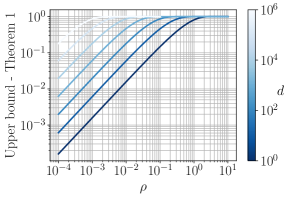
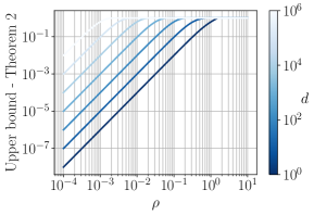
Figure 2: Behavior of the quantitative bounds shown in Theorems 1 and 2 w.r.t. $\rho$ in log-log scale for a set of dimensions $d$. The other quantities appearing in the bounds have been set to 1.

Theorem 1 is easily extended to the case where the initial density $\pi$ is expressed as a product of several terms. If $\pi$ stands for the pdf associated to the variable $\boldsymbol{\theta}$, this boils down to considering

$$\pi(\boldsymbol{\theta})\propto\prod_{j=1}^{J}\pi_{j}(\boldsymbol{\theta})\propto\exp\left(-\sum_{j=1}^{J}f_{j}(\boldsymbol{\theta})\right),$$ (31)

where for all $j\in[J]$, $f_{j}\mathrel{\mathop{\mathchar 58\relax}}\mathbb{R}^{d}\rightarrow\mathbb{R}$, and a natural generalization of AXDA when applied to each $\pi_{j}$, which writes

$$\pi_{\rho}(\boldsymbol{\theta},\mathbf{z}_{1\mathrel{\mathop{\mathchar 58\relax}}J})\propto\prod_{j=1}^{J}\pi_{j}(\mathbf{z}_{j})\kappa_{\rho_{j}}(\mathbf{z}_{j};\boldsymbol{\theta})\propto\exp\left(-\sum_{j=1}^{J}f_{j}(\mathbf{z}_{j})+\dfrac{1}{2\rho_{j}^{2}}\left\|\mathbf{z}_{j}-\boldsymbol{\theta}\right\|_{2}^{2}\right).$$ (32)

Under this product form, we have the following corollary.

Corollary 3.

For all $j\in[J]$, let $f_{j}$ satisfy $(A_{1})$. Then,

$$\left\|\pi_{\rho}-\pi\right\|_{\mathrm{TV}}\leq 1-\prod_{j=1}^{J}\Delta_{d}^{(j)}(\rho_{j}),$$ (33)

where $\Delta_{d}^{(j)}(\rho_{j})=D_{-d}(L_{f_{j}}\rho_{j})/D_{-d}(-L_{f_{j}}\rho_{j})$.

Unfortunately, Theorem 2 cannot be extended to the multiple splitting scenario. We are nevertheless confident that quantitative bounds can be found with different proof techniques but this task goes beyond the scope of this paper.

4.3.3 Uniform bounds on potentials

From an optimization point of view, it is quite common to consider potential functions associated to densities. For such applications, we give hereafter a quantitative uniform bound on the difference between the potential functions associated to $\pi$ and $\pi_{\rho}$. Similarly to the definition of the potential function $f$ in (1), we define the potential function $f_{\rho}$ associated to the approximate marginal $\pi_{\rho}$ in (3), for all $\boldsymbol{\theta}\in\mathbb{R}^{d}$, by

$$f_{\rho}(\boldsymbol{\theta})=-\log\int_{\mathbb{R}^{d}}\exp\left(-f(\mathbf{z})\right)\kappa_{\rho}(\mathbf{z},\boldsymbol{\theta})\mathrm{d}\mathbf{z}.$$ (34)

By considering a Gaussian smoothing kernel $\kappa_{\rho}$, the potential $f_{\rho}$ becomes

$$f_{\rho}(\boldsymbol{\theta})=-\log\int_{\mathbb{R}^{d}}\exp\left(-f(\mathbf{z})-\dfrac{1}{2\rho^{2}}\left\|\mathbf{z}-\boldsymbol{\theta}\right\|_{2}^{2}\right)\mathrm{d}\mathbf{z}+\frac{d}{2}\log(2\pi\rho^{2}).$$ (35)

Note that $f_{\rho}(\boldsymbol{\theta})$ appears as a regularized version of $f(\boldsymbol{\theta})$.

Proposition 4.

Let $f$ satisfy $(A_{1})$. Then, for all $\boldsymbol{\theta}\in\mathbb{R}^{d}$,

$$L_{\rho}\leq f_{\rho}(\boldsymbol{\theta})-f(\boldsymbol{\theta})\leq U_{\rho},$$ (36)

with

$$L_{\rho}=\log N_{\rho}-\log D_{-d}(-L_{f}\rho),$$ (37)

$$U_{\rho}=\log N_{\rho}-\log D_{-d}(L_{f}\rho),$$ (38)

and

$$N_{\rho}=\dfrac{2^{d/2-1}\Gamma\left(d/2\right)}{\Gamma(d)\exp\left(L_{f}^{2}\rho^{2}/4\right)}.$$ (39)

It is easily observed that these bounds are informative in the limiting case $\rho\rightarrow 0$ since they both tend towards zero.

4.3.4 Uniform bounds on credibility regions

When $\pi$ stands for the density associated to a posterior distribution, one advantage of Bayesian analysis is its ability to derive the underlying probability distribution of the variable of interest $\boldsymbol{\theta}$ and thereby to provide credibility information under this distribution. This uncertainty information is particularly relevant and essential for real-world applications. Since the marginal $\pi_{\rho}$ stands for an approximation of the original target distribution $\pi$, it is important to control the credibility regions under $\pi_{\rho}$ w.r.t. those drawn under $\pi$. The control in total variation distance given by Theorem 1 is already a good indication. However, it is possible to quantify more precisely the difference between the credible regions (Robert 2001) with confidence level ($1-\alpha$) under $\pi_{\rho}$ and $\pi$, as stated below.

Proposition 5.

Let $\pi$ be a posterior distribution associated to $\boldsymbol{\theta}$ and $f$ such that $(A_{1})$ is verified. Let $\mathcal{C}_{\alpha}^{\rho}$ an arbitrary $(1-\alpha)$-credibility region under $\pi_{\rho}$, that is $\mathbb{P}_{\pi_{\rho}\text{}}\left(\boldsymbol{\theta}\in\mathcal{C}_{\alpha}^{\rho}\right)=1-\alpha$ with $\alpha\in(0,1)$. Then,

$$(1-\alpha)\dfrac{N_{\rho}}{D_{-d}(-L_{f}\rho)}\leq\int_{\mathcal{C}_{\alpha}^{\rho}}\pi(\boldsymbol{\theta})\mathrm{d}\boldsymbol{\theta}\leq\min\left(1,(1-\alpha)\dfrac{N_{\rho}}{D_{-d}(L_{f}\rho)}\right),$$ (40)

where $N_{\rho}$ is defined in (39).

Proposition 5 states that the coverage of $\pi$ under $\mathcal{C}_{\alpha}^{\rho}$ can be determined for a fixed value of $\rho$. Thus, it is even possible to obtain a theoretical comprehensive description of $\mathcal{C}_{\alpha}^{\rho}$ w.r.t. the initial target density $\pi$ before conducting an AXDA-based inference. The bounds in (40) permit to choose a parameter $\rho$ in order to ensure a prescribed coverage property. The behavior of these bounds w.r.t. $\rho$ is the same as in Section 4.3.2, i.e., linear behavior w.r.t. $\rho$ when this parameter is sufficiently small.

5 Numerical illustrations

This section illustrates the quantitative results shown in Sections 4.1 and 4.3 on three different examples which classically appear in statistical signal processing and machine learning. As shown in Table 1, the bias induced by considering $\pi_{\rho}$ is mostly driven by the value of the tolerance parameter $\rho$ rather than by the choice of $\kappa_{\rho}$. Hence, for simplicity, most of the numerical illustrations hereafter consider the case where $\kappa_{\rho}$ is a Gaussian smoothing kernel. Additional illustrations can be found in the online supplementary material.

5.1 Multivariate Gaussian example

We start by performing a sanity check with the simple case where $\pi$ stands for a multivariate Gaussian density that is

$$\pi(\boldsymbol{\theta})=\mathcal{N}(\boldsymbol{\theta}|\boldsymbol{\mu},\mathbf{\Sigma}),$$ (41)

where $\mathbf{\Sigma}$ is assumed to be positive definite. If $\kappa_{\rho}(\cdot,\boldsymbol{\theta})$ is taken to be Gaussian density with mean $\boldsymbol{\theta}$ and covariance matrix $\rho^{2}\mathbf{I}_{d}$, then one can show that

$$\pi_{\rho}(\boldsymbol{\theta})=\mathcal{N}(\boldsymbol{\theta}|\boldsymbol{\mu},\mathbf{\Sigma}+\rho^{2}\mathbf{I}_{d}).$$ (42)

In particular, let consider the univariate setting, that is $\Theta=\mathbb{R}$, $\mathbf{\Sigma}=\sigma^{2}$. In this case, the variance under $\pi_{\rho}$ is $\sigma^{2}+\rho^{2}$ and simply corresponds to the variance under $\pi$ inflated by a factor $\rho^{2}$. Therefore, the approximation will be reasonable if $\rho^{2}/\sigma^{2}$ is sufficiently small, see Figure 3. In this Figure, we also show the approximation induced by considering a uniform kernel instead of a Gaussian one. The smoothing via the uniform kernel performs slightly better than Gaussian smoothing due to its lower variance. In both cases, the approximation is reasonable for small $\rho$ although $\pi_{\rho}$, built with a uniform kernel, no longer belongs to the Gaussian family.

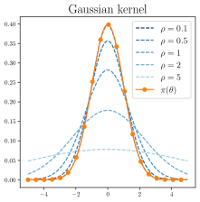
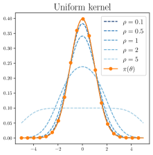
Figure 3: Bias between $\pi_{\rho}$ and $\pi$ in the case $\Theta=\mathbb{R}$, $\pi=\mathcal{N}(\mu,\sigma^{2})$ with $\mu=0$ and $\sigma=1$. (left) $\pi_{\rho}$ is built with a Gaussian kernel $\mathcal{N}(0,\rho^{2})$ and (right) with a uniform kernel on $[-\rho,\rho]$. Note that the curves associated to $\pi$ and $\pi_{\rho}$ for $\rho=0.1$ are overlapping.

In order to illustrate the proposed upper bounds on both 2-Wasserstein and total variation distances, we consider a covariance matrix $\mathbf{\Sigma}$ which stands for a squared exponential matrix commonly used in applications involving Gaussian processes (Higdon 2007) and which writes

$$\Sigma_{ij}=2\exp\left(-\dfrac{(s_{i}-s_{j})^{2}}{2a^{2}}\right)+10^{-6}\delta_{ij},\forall i,j\in[d]$$ (43)

where $a=1.5$, $s_{i,i\in[d]}$ are regularly spaced scalars on $[-3,3]$ and $\delta_{ij}=1$ if $i=j$ and zero otherwise.

Figure 4 shows the behavior of the quantitative bounds derived in Proposition 2 and Theorem 2 for $d\in\{10,100\}$. The Gaussian case allows to compute exactly $W_{2}(\pi,\pi_{\rho})$ by noting that $W_{2}^{2}(\pi,\pi_{\rho})=\mathrm{Trace}(\mathbf{\Sigma}+\rho^{2}\mathbf{I}_{d}-2\rho\mathbf{\Sigma}^{1/2})$. On the other hand, $\left\|\pi-\pi_{\rho}\right\|_{\mathrm{TV}}$ has been estimated by using a Monte Carlo approximation. One can note that the general upper bound on the 2-Wasserstein distance is quite conservative for small $\rho$ since it does not catch the behavior in $\mathcal{O}(\rho^{2})$ when $\rho$ is small. This is essentially due to the fact that this bound only assumes a finite moment property and does not require any regularity assumptions on $\pi$ such as differentiability or strong convexity of its potential. On the contrary, the bound on the total variation distance, derived under stronger assumptions, manages to achieve a rate of the order $\mathcal{O}(\rho^{2})$ for small $\rho$.

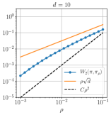
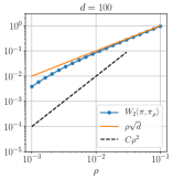
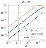
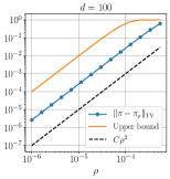
Figure 4: For $d\in\{10,100\}$, illustration of the quantitative bounds (20) and (29) associated to 2-Wasserstein and total variation distances, respectively. The decay in $\mathcal{O}(\rho^{2})$ is shown via the dashed line $C\rho^{2}$ where $C$ is a constant.

5.2 Sparse linear regression

We study here a generalized version of the least absolute shrinkage and selection operator (lasso) regression problem analyzed by Park and Casella (2008). We assume a standard linear regression problem where centered observations $\mathbf{y}\in\mathbb{R}^{n}$ are related to the unknown parameters $\boldsymbol{\theta}\in\mathbb{R}^{d}$ via the model $\mathbf{y}=\mathbf{X}\boldsymbol{\theta}+\boldsymbol{\varepsilon}$, where $\mathbf{X}\in\mathbb{R}^{n\times d}$ stands for a known standardized design matrix and $\boldsymbol{\varepsilon}\sim\mathcal{N}(\mathbf{0}_{n},\sigma^{2}\mathbf{I}_{n})$. By considering a generalized Laplacian prior distribution for $\boldsymbol{\theta}$, the target posterior distribution has density for all $\boldsymbol{\theta}\in\mathbb{R}^{d}$,

$$\pi(\boldsymbol{\theta})\triangleq\pi(\boldsymbol{\theta}|\mathbf{y})\propto\exp\left(-\dfrac{1}{2\sigma^{2}}\left\|\mathbf{y}-\mathbf{X}\boldsymbol{\theta}\right\|_{2}^{2}-g(\mathbf{B}\boldsymbol{\theta})\right)$$ (44)

where $g(\mathbf{B}\boldsymbol{\theta})=\tau\left\|\mathbf{B}\boldsymbol{\theta}\right\|_{1}$ with $\tau>0$ and $\mathbf{B}\in\mathbb{R}^{k\times d}$ an arbitrary matrix acting on $\boldsymbol{\theta}$. The choice of such a prior may promote a form of sparsity (lasso). For instance, this matrix $\mathbf{B}$ might stand for a $p$-th order difference operator (Bredies et al. 2010) which is highly used in signal and image processing problems. As an archetypal example, the case $p=1$ leads to the well-known total variation regularization function (Chambolle et al. 2010) used to recover piecewise constant signals.

Note that because of the presence of the matrix $\mathbf{B}$, finding an exact data augmentation leading to an efficient sampling scheme is not possible for the general case $\mathbf{B}\neq\mathbf{I}_{d}$. Instead, an AXDA model makes the posterior sampling task possible. Indeed, by regularizing the prior with a Gaussian term, the joint density $\pi_{\rho}$ writes

$$\pi_{\rho}(\boldsymbol{\theta},\mathbf{z})\propto\exp\left(-\dfrac{1}{2\sigma^{2}}\left\|\mathbf{y}-\mathbf{X}\boldsymbol{\theta}\right\|_{2}^{2}-g(\mathbf{z})-\dfrac{1}{2\rho^{2}}\left\|\mathbf{Bx}-\mathbf{z}\right\|_{2}^{2}\right).$$ (45)

By resorting to a Gibbs algorithm to sample from (45), one can now use a simple data augmentation scheme (Park and Casella 2008) to sample from the $\mathbf{z}$-conditional. On the other hand, sampling from the $\boldsymbol{\theta}$-conditional, which is a multivariate Gaussian distribution, can be undertaken efficiently with state-of-the-art approaches (Papandreou and Yuille 2010; Barbos et al. 2017; Marnissi et al. 2018).

In this specific case, the potential $g_{\rho}$ associated to the smoothed prior distribution (see (35)) has a closed-form expression given for all $\boldsymbol{\theta}\in\mathbb{R}^{d}$, by

$$g_{\rho}(\boldsymbol{\theta}) =\dfrac{k}{2}\log(2\pi\rho^{2})-\log\prod_{i=1}^{k}\displaystyle\int_{\mathbb{R}}\exp\left(-\tau|z_{i}|-\dfrac{1}{2\rho^{2}}(\mathbf{b}_{i}^{T}\boldsymbol{\theta}-z_{i})^{2}\right)\mathrm{d}z_{i}$$

$$=\dfrac{k}{2}\log(2\pi\rho^{2})$$ (46)

$$-\log\prod_{i=1}^{k}\left(a(\boldsymbol{\theta})\left[\exp\left(b(\boldsymbol{\theta})^{2}\right)\left\{1-\mathrm{erf}(b(\boldsymbol{\theta}))\right\}+\exp\left(c(\boldsymbol{\theta})^{2}\right)\left\{1-\mathrm{erf}(c(\boldsymbol{\theta}))\right\}\right]\right)$$ (47)

with $a(\boldsymbol{\theta})=\sqrt{\pi\rho^{2}/2}\exp\left(-(\mathbf{b}_{i}^{T}\boldsymbol{\theta})^{2}/(2\rho^{2})\right)$, $b(\boldsymbol{\theta})=\sqrt{\rho^{2}/2}(\tau-\mathbf{b}_{i}^{T}\boldsymbol{\theta}/\rho^{2})$, $c(\boldsymbol{\theta})=\sqrt{\rho^{2}/2}(\tau+\mathbf{b}_{i}^{T}\boldsymbol{\theta}/\rho^{2})$ and $\mathbf{b}_{i}\in\mathbb{R}^{d}$ standing for the $i$-th row of $\mathbf{B}$. Note that in more general cases where $g_{\rho}$ has no closed form, one can estimate it by a Monte Carlo approximation.

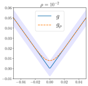
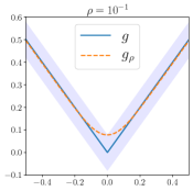
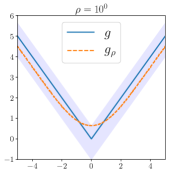
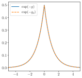
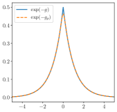
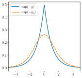
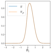
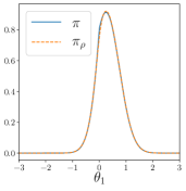
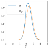
Figure 5: From left to right, $\rho=0.01$, $\rho=0.1$ and $\rho=1$. (1st row) Behaviors of $g$ (blue) and $g_{\rho}$ (orange) where the contours of the shaded area correspond to $g+L_{\rho}$ and $g+U_{\rho}$; (2nd row) the corresponding normalized smoothed prior densities proportional to $\exp(-g)$ and $\exp(-g_{\rho})$; (3rd row) posterior densities $\pi_{\rho}$ w.r.t. $\rho$.

Figure 5 shows the behavior of the regularized potential $g_{\rho}$ defined in (47) for several values of the parameter $\rho$ along with the associated smoothed prior and posterior distributions. For simplicity and pedagogical reasons, the univariate case corresponding to $\boldsymbol{\theta}=\theta_{1}\in\mathbb{R}$ and $\mathbf{B}=1$ has been considered. The regularization parameter $\tau$ has been set to $\tau=1$. The contours of the shaded area correspond to $g+L_{\rho}$ and $g+U_{\rho}$. The potential $g_{\rho}$ is a smooth approximation of the potential $g$ associated to the initial prior as expected, see Property iv) in Proposition 1. Note that the inequalities derived in (36) are verified. Although this approximation seems similar to the Moreau-Yosida regularization of a non-smooth potential function (Combettes and Pesquet 2011), the rationale behind this approximation is different. Indeed, the Moreau-Yosida envelope stands for a particular instance of the infimal convolution between two convex functions (an initial potential and a Gaussian one). On the other hand, $g_{\rho}$ is the potential associated to a smoothed density obtained by convolution with a Gaussian kernel. In addition, the third row of Figure 5 shows the form of the posterior of $\theta_{1}$ defined in (45) for $y=1$, $x=2$ and $\sigma=1$ and derived from the smoothed prior distributions shown in Figure 5. For sufficiently small values of $\rho$, the marginal $\pi_{\rho}$ stands for a quite accurate approximation of the original target $\pi$.

Table 2: Illustration of the bound derived in (40) for the marginal posterior $\pi_{\rho}$ depicted in Section 5.2. The (1-$\alpha$)-credibility intervals $\mathcal{C}_{\alpha}$ and $\mathcal{C}_{\alpha}^{\rho}$ are the highest posterior density regions associated to each density with $\alpha=0.05$.

$\rho$	$\mathcal{C}_{\alpha}$	$\mathcal{C}^{\rho}_{\alpha}$	$\int_{\mathcal{C}_{\alpha}^{\rho}}\pi(\theta_{1})\mathrm{d}\theta_{1}$	$\mathcal{I}_{\alpha}^{\rho}$
$10^{-3}$	[-0.47,1.24]	[-0.47,1.24]	0.95	[0.949,0.951]
$10^{-2}$	idem	[-0.47,1.24]	0.95	[0.948,0.952]
$10^{-1}$	idem	[-0.47,1.24]	0.95	[0.88,1]
$10^{0}$	idem	[-0.47,1.37]	0.96	[0.34,1]

Table 2 illustrates the bounds derived in (40) for $\rho\in\left\{1,10^{-1},10^{-2},10^{-3}\right\}$. For each case, the values of the bounds are summarized in the interval

$$\mathcal{I}_{\alpha}^{\rho}=[(1-\alpha)N_{\rho}/D_{-d}(-L_{f}\rho),\min(1,(1-\alpha)N_{\rho}/D_{-d}(L_{f}\rho)],$$ (48)

and the real coverage $\int_{\mathcal{C}_{\alpha}^{\rho}}\pi(\theta_{1})\mathrm{d}\theta_{1}$ is also reported. The (1-$\alpha$)-credibility intervals $\mathcal{C}_{\alpha}$ and $\mathcal{C}_{\alpha}^{\rho}$ have been chosen to be the highest posterior density regions associated to each density with $\alpha=0.05$. Note that the theoretical coverage interval $\mathcal{I}_{\alpha}^{\rho}$ becomes informative only if $\rho$ is sufficiently small which is not surprising since the assumptions on the potential of $\pi_{\rho}$ are weak. Indeed, the form of the density (e.g. symmetry or unimodality) is not taken into account in the derived bounds. Regarding the empirical value of the coverage $\int_{\mathcal{C}_{\alpha}^{\rho}}\pi(\theta_{1})\mathrm{d}\theta_{1}$, we emphasize that the marginal $\pi_{\rho}$ stands for a conservative approximation of $\pi$ in this example. Indeed, in each case, the (1-$\alpha$)-credibility interval under $\pi_{\rho}$ denoted $\mathcal{C}_{\alpha}^{\rho}$ covers at least $100(1-\alpha)$% of the probability mass under $\pi$.

5.3 Illustration on an image inpainting problem

We illustrate here the correctness of the proposed approach on a multidimensional and non-Gaussian example which classically appears in image processing. To this purpose, we consider the observation of a damaged and noisy image $\mathbf{y}\in\mathbb{R}^{n}$ (represented as a vector by lexicographic ordering) related to the unknown original image $\boldsymbol{\theta}\in\mathbb{R}^{d}$ by the linear model

$$\mathbf{y}=\mathbf{H}\boldsymbol{\theta}+\boldsymbol{\varepsilon},\quad\boldsymbol{\varepsilon}\sim\mathcal{N}(\mathbf{0}_{n},\sigma^{2}\mathbf{I}_{n}),$$ (49)

where $n<d$, $\mathbf{H}\in\mathbb{R}^{n\times d}$ stands for a decimation binary matrix. The dimension $d$ being typically large (e.g., $10^{3}\leq d\leq 10^{9}$), these problems require scalable inference algorithms. Since the matrix $\mathbf{H}$ is not invertible, the linear inverse problem (49) is ill-posed. To cope with this issue, we assign the total variation prior distribution to the unknown parameter $\boldsymbol{\theta}$, leading to the posterior distribution

$$\pi(\boldsymbol{\theta}|\mathbf{y})\propto\exp\left(-\frac{1}{2\sigma^{2}}\left\|\mathbf{y}-\mathbf{H}\boldsymbol{\theta}\right\|_{2}^{2}-\tau\sum_{1\leq i\leq d}\left\|(\mathbf{D}\boldsymbol{\theta})_{i}\right\|_{2}\right),$$ (50)

where $\tau>0$ is a regularization parameter, $\mathbf{D}\boldsymbol{\theta}=(\mathbf{D}_{1}\boldsymbol{\theta},\mathbf{D}_{2}\boldsymbol{\theta})\in\mathbb{R}^{2\times d}$ is the two-dimensional discrete gradient associated to the image $\boldsymbol{\theta}$ and the notation $\mathbf{M}_{i}$ stands for the $i$-th column of the matrix $\mathbf{M}$, see Chambolle et al. (2010) for more details about the total variation regularization. The presence of the operator $\mathbf{D}$ and the non-differentiability of the total variation norm rule out the use of common data augmentation schemes and simulation-based algorithms (e.g., Hamiltonian and Langevin Monte Carlo methods). Possible surrogates are proximal MCMC methods (Pereyra 2016; Durmus et al. 2018) which replace the non-differentiable posterior distribution by a smooth approximation based on the proximity operator (Combettes and Pesquet 2011) of the total variation norm. However, the latter does not admit a closed-form expression and iterative routines are commonly used to approximate the latter (Chambolle 2004) leading to higher computational costs.

To mitigate these issues, we propose to rely on a particular instance of AXDA by smoothing the total variation prior with a Gaussian term, leading to the approximate joint posterior density

$$\pi_{\rho}(\boldsymbol{\theta},\mathbf{z}|\mathbf{y})\propto\exp\left(-\frac{1}{2\sigma^{2}}\left\|\mathbf{y}-\mathbf{H}\boldsymbol{\theta}\right\|_{2}^{2}-\tau\sum_{1\leq i\leq d}\left\|\mathbf{Z}_{i}\right\|_{2}-\frac{1}{2\rho^{2}}\left\|\mathbf{Z}-\mathbf{D}\boldsymbol{\theta}\right\|_{2}^{2}\right),$$ (51)

where $\mathbf{Z}=(\mathbf{z}_{1},\mathbf{z}_{2})\in\mathbb{R}^{2\times d}$. By relying on (51), the inference is now simplified and can be conducted with a Gibbs sampler, see Section 4 in the supplementary material. Since $\mathrm{ker}(\mathbf{H})\cap\mathrm{ker}(\mathbf{D})=\{\mathbf{0}_{d}\}$, the conditional posterior distribution of $\boldsymbol{\theta}$ is a non-degenerate multivariate Gaussian distribution. Samples from the latter can be obtained efficiently with the two-dimensional discrete Fourier transform by exploiting the periodic boundary conditions for $\boldsymbol{\theta}$ (Wang et al. 2008; Marnissi et al. 2018). On the other hand, samples from $\pi_{\rho}(\mathbf{Z}|\boldsymbol{\theta})$ can be drawn efficiently using exact data augmentation, see Kyung et al. (2010). All the inference details are given in Section 4 of the supplementary material.

We illustrate the proposed approximate model $\pi_{\rho}$ by considering the Shepp-Logan phantom magnectic resonance image of size $100\times 100$ ($d=10^{4}$), see Figure 6. We artifically damaged and added noise to this image to build a noisy observation $\mathbf{y}$ consisting of 90% randomly selected pixels of the initial image. The standard deviation of the Gaussian noise and the regularization parameter have been set to $\sigma=7\times 10^{-2}$ (corresponding to a SNR of 58dB) and $\tau=5$, respectively. The tolerance parameter has been set to $\rho=0.1$.

In order to assess the bias of the proposed approach, we implemented the Moreau-Yosida Metropolis-adjusted Langevin algorithm (MYMALA) of Durmus et al. (2018), specifically designed to sample exactly from high-dimensional and non-smooth posterior distributions. For all the MCMC algorithms, the initialization has been set to $\boldsymbol{\theta}^{[0]}=\mathbf{0}_{d}$. We generated $10^{5}$ samples and kept the last $5\times 10^{4}$ ones.

Figure 6 shows the minimum mean square estimate (MMSE) under $\pi_{\rho}$ along with the original image. One can denote that the MMSE under $\pi_{\rho}$ is visually similar to the original image and hence coherent with the reconstruction task. The relative residual error between the former and the MMSE under $\pi$ is of order 2%. The main differences are located on the boundaries of the image, as depicted in the figure on the left which shows the absolute difference between the pixels of the two posterior means $\mathbb{E}_{\pi}(\boldsymbol{\theta})$ and $\mathbb{E}_{\pi_{\rho}}(\boldsymbol{\theta})$.

Figure 6: From left to right: original image, minimum mean square estimate (MMSE) under $\pi_{\rho}$ and absolute bias between the posterior means under $\pi_{\rho}$ and $\pi$.

To emphasize the correctness of the proposed approach beyond the comparision between pointwise estimates, we also paid attention to the comparison between posterior credibility sets induced by both $\pi$ and $\pi_{\rho}$. To this purpose, we considered the highest posterior density region given by

$$\mathcal{C}_{\alpha}^{\star}=\{\boldsymbol{\theta}\in\mathbb{R}^{d}\ |\ f(\boldsymbol{\theta})\leq\gamma_{\alpha}\},$$ (52)

where $\gamma_{\alpha}\in\mathbb{R}$ is such that $\int_{\mathcal{C}_{\alpha}^{\star}}\pi(\boldsymbol{\theta}|\mathbf{y})\mathrm{d}\boldsymbol{\theta}=1-\alpha$ and $f$ is the potential function associated to $\pi(\boldsymbol{\theta}|\mathbf{y})$.

Figure 7 shows the different values of the scalar summary $\gamma_{\alpha}$ estimated using $\pi$ and the scalar $\gamma_{\alpha}^{\rho}$ estimated using $\pi_{\rho}$ for $\alpha\in[0.01,0.99]$. Note that the approximation error associated to $\gamma_{\alpha}$ is of order 2.6% whatever the value of $\alpha$, which supports the use of $\pi_{\rho}$ to conduct Bayesian uncertainty analysis in this problem. After the burn-in period, the efficiency of the Gibbs algorithm used to sample from $\pi_{\rho}$ has been measured by comparing the effective sample size (ESS) associated to the slowest component of $\boldsymbol{\theta}$ to the one obtained with MYMALA. We found that the two ESS were roughly similar but the cost per iteration of the Gibbs sampler (0.079 sec/iteration) is almost two times lower than that of MYMALA (0.144 sec/iteration). In addition, the number of iterations required to reach high-probability regions is much less important for the Gibbs sampler than for MYMALA, showing the interest of AXDA, see Figure 7.

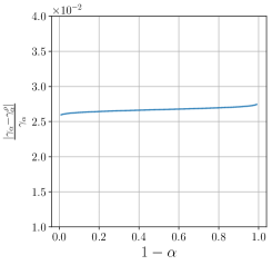
Figure 7: (left) relative error between the threshold value estimated with $\pi$ denoted $\gamma_{\alpha}$ and the one estimated with $\pi_{\rho}$ denoted $\gamma_{\alpha}^{\rho}$ and (right) Potential $f=-\log\pi$ w.r.t. the number of iterations $t$ for both MYMALA and the Gibbs sampler targetting $\pi_{\rho}$.

6 Conclusion

This paper presented a unifying framework for asymptotically exact data augmentation (AXDA) schemes. AXDA introduces approximate densities in order to simplify the inference. By building on existing works which considered special instances of AXDA, we illustrate potential benefits that can be inherited by the proposed framework such as distributed computations, robustness or sophisticated inference schemes from the ABC literature. On top of these qualitative properties, we derived a set of theoretical guarantees on the bias involved in the proposed methodology. The latter encompass a large class of AXDA models and a detailed non-asymptotic analysis has been done for Gaussian smoothing. These results have been illustrated on several cases that can arise in statistical learning or signal processing showing the broad scope of application of the proposed approach. In practice, we emphasize that AXDA models can remarkably improve the inference task in big data and high-dimensional settings. In summary, at the price of an approximation which comes with theoretical guarantees, AXDA approaches appear to be a general, systematic and efficient way to conduct simple inference in a wide variety of large-scale problems. They provide accurate estimates with relevant confidence intervals that are crucial in many applications, in particular when no ground truth is available.

Appendix 1 Proofs

1.1 Proof of Proposition 1

Property i) follows from the fact that $\pi_{\rho}$ stands for a convolution integral between $\pi$ and $\kappa_{\rho}$, i.e. $\pi_{\rho}=\pi\ast\kappa_{\rho}$. Therefore, the expectation and variance under $\pi_{\rho}$ are the sum of the expectations and variances of two independent random variables under $\pi$ and $\kappa_{\rho}$ respectively. Property ii) follows directly from (Folland 1999, Proposition 8.6). Property iii) follows from the fact that log-concavity is preserved by convolution of distributions (Dharmadhikari and Joag-Dev 1988, Theorem 2.18). Finally, Property iv) follows from the dominated convergence theorem since $\pi\in L^{1}$, $\kappa_{\rho}\in\mathcal{C}^{\infty}(\mathbb{R}^{d})$ and for all $k\geq 0$, $|\partial^{k}\kappa_{\rho}|\leq C_{k}$ (Folland 1999, Proposition 8.10).

1.2 Proof of Proposition 2

The proof can be found in Ambrosio et al. (2008, Lemma 7.1.10). Since it is quite short, we recall it hereafter for completeness. We have

$$W_{p}^{p}(\pi,\pi_{\rho}) =\min_{\mu}\left\{\int_{\mathbb{R}^{d}}\int_{\mathbb{R}^{d}}\left\|\boldsymbol{\theta}-\mathbf{z}\right\|_{2}^{p}\mathrm{d}\mu(\boldsymbol{\theta},\mathbf{z});\mu\in\Gamma(\pi_{\rho},\pi)\right\}$$ (53)

$$\leq\int_{\mathbb{R}^{d}}\int_{\mathbb{R}^{d}}\left\|\boldsymbol{\theta}-\mathbf{z}\right\|_{2}^{p}\pi_{\rho}(\boldsymbol{\theta},\mathbf{z})\mathrm{d}\boldsymbol{\theta}\mathrm{d}\mathbf{z}$$ (54)

$$=\int_{\mathbb{R}^{d}}\int_{\mathbb{R}^{d}}\left\|\boldsymbol{\theta}-\mathbf{z}\right\|_{2}^{p}\kappa_{\rho}(\mathbf{z},\boldsymbol{\theta})\pi(\mathbf{z})\mathrm{d}\boldsymbol{\theta}\mathrm{d}\mathbf{z}$$ (55)

$$=\rho^{-d}\int_{\mathbb{R}^{d}}\int_{\mathbb{R}^{d}}\left\|\boldsymbol{\theta}-\mathbf{z}\right\|_{2}^{p}K(\rho^{-1}(\boldsymbol{\theta}-\mathbf{z}))\pi(\mathbf{z})\mathrm{d}\boldsymbol{\theta}\mathrm{d}\mathbf{z}$$ (56)

$$=\rho^{p}\int_{\mathbb{R}^{d}}\left\|\mathbf{u}\right\|_{2}^{p}K(\mathbf{u})\mathrm{d}\mathbf{u}\int_{\mathbb{R}^{d}}\pi(\mathbf{z})\mathrm{d}\mathbf{z}$$ (57)

$$=\rho^{p}\int_{\mathbb{R}^{d}}\left\|\mathbf{u}\right\|_{2}^{p}K(\mathbf{u})\mathrm{d}\mathbf{u}.$$ (58)

1.3 Proof of Proposition 3

Let $\boldsymbol{\theta}\in\mathbb{R}^{d}$. Since $\pi$ has been assumed to be analytic and twice differentiable with $\mathbf{H}_{\pi}$ being continuous, there exists $\tilde{\boldsymbol{\theta}}$ lying between $\boldsymbol{\theta}$ and $\boldsymbol{\theta}-\sqrt{\rho}\mathbf{u}$ such that

$$\pi_{\rho}(\boldsymbol{\theta}) =\int_{\mathbb{R}^{d}}\pi(\mathbf{z})\kappa_{\rho}(\mathbf{z},\boldsymbol{\theta})\mathrm{d}\mathbf{z}$$ (59)

$$=\dfrac{\displaystyle\int_{\mathbb{R}^{d}}\pi(\boldsymbol{\theta}-\sqrt{\rho}\mathbf{u})\exp\left(-\dfrac{d_{\psi}(\boldsymbol{\theta}-\sqrt{\rho}\mathbf{u},\boldsymbol{\theta})}{\rho}\right)\mathrm{d}\mathbf{u}}{\displaystyle\int_{\mathbb{R}^{d}}\exp\left(-\dfrac{d_{\psi}(\boldsymbol{\theta}-\sqrt{\rho}\mathbf{u},\boldsymbol{\theta})}{\rho}\right)\mathrm{d}\mathbf{u}}$$ (60)

$$=\dfrac{\displaystyle\int_{\mathbb{R}^{d}}\left[\pi(\boldsymbol{\theta})-\sqrt{\rho}\nabla\pi(\boldsymbol{\theta})^{T}\mathbf{u}+\frac{\rho}{2}\mathbf{u}^{T}\mathbf{H}_{\pi}(\boldsymbol{\tilde{\theta}})\mathbf{u}\right]\exp\left(-\dfrac{d_{\psi}(\boldsymbol{\theta}-\sqrt{\rho}\mathbf{u},\boldsymbol{\theta})}{\rho}\right)\mathrm{d}\mathbf{u}}{\displaystyle\int_{\mathbb{R}^{d}}\exp\left(-\dfrac{d_{\psi}(\boldsymbol{\theta}-\sqrt{\rho}\mathbf{u},\boldsymbol{\theta})}{\rho}\right)\mathrm{d}\mathbf{u}},$$ (61)

where $\mathbf{H}_{\pi}$ stands for the Hessian matrix of $\pi$.

It follows that

$$\pi_{\rho}(\boldsymbol{\theta}) =\pi(\boldsymbol{\theta})$$ (62)

$$-\sqrt{\rho}\nabla\pi(\boldsymbol{\theta})^{T}\int_{\mathbb{R}^{d}}\mathbf{u}\frac{\exp\left(-\dfrac{d_{\psi}(\boldsymbol{\theta}-\sqrt{\rho}\mathbf{u},\boldsymbol{\theta})}{\rho}\right)\mathrm{d}\mathbf{u}}{\displaystyle\int_{\mathbb{R}^{d}}\exp\left(-\dfrac{d_{\psi}(\boldsymbol{\theta}-\sqrt{\rho}\mathbf{u},\boldsymbol{\theta})}{\rho}\right)\mathrm{d}\mathbf{u}}$$ (63)

$$+\frac{\rho}{2}\dfrac{\displaystyle\int_{\mathbb{R}^{d}}\mathbf{u}^{T}\mathbf{H}_{\pi}(\tilde{\boldsymbol{\theta}})\mathbf{u}\exp\left(-\dfrac{d_{\psi}(\boldsymbol{\theta}-\sqrt{\rho}\mathbf{u},\boldsymbol{\theta})}{\rho}\right)\mathrm{d}\mathbf{u}}{\displaystyle\int_{\mathbb{R}^{d}}\exp\left(-\dfrac{d_{\psi}(\boldsymbol{\theta}-\sqrt{\rho}\mathbf{u},\boldsymbol{\theta})}{\rho}\right)\mathrm{d}\mathbf{u}}$$ (64)

We now show that (63) $=O(\sqrt{\rho})$ and (64) $=\mathcal{O}(\rho)$. To this purpose, we use the analyticity and two times differentiability of $d_{\psi}$ w.r.t. to its first argument and the continuity of $\mathbf{H}_{d_{\psi}}$. By definition of the Bregman divergence (see Definition 1 in the main paper), $d_{\psi}(\boldsymbol{\theta},\boldsymbol{\theta})=0$ and $\nabla_{\mathbf{z}}d_{\psi}(\mathbf{z},\boldsymbol{\theta})\Bigr{|}_{\begin{subarray}{c}\mathbf{z}=\boldsymbol{\theta}\end{subarray}}=\mathbf{0}_{d}$ so that, for all $\mathbf{u}\in\mathbb{R}^{d}$,

$$d_{\psi}(\boldsymbol{\theta}-\sqrt{\rho}\mathbf{u},\boldsymbol{\theta})=\frac{\rho}{2}\mathbf{u}^{T}\mathbf{H}_{d_{\psi}}(\boldsymbol{\theta}^{\prime})\mathbf{u},$$ (65)

where $\boldsymbol{\theta}^{\prime}$ lies between $\boldsymbol{\theta}$ and $\boldsymbol{\theta}-\sqrt{\rho}\mathbf{u}$.

We first prove (64) $=\mathcal{O}(\rho)$. Using (65), we can re-write (64) as

$$(12) =\frac{\rho}{2}\dfrac{\displaystyle\int_{\mathbb{R}^{d}}\mathbf{u}^{T}\mathbf{H}_{\pi}(\tilde{\boldsymbol{\theta}})\mathbf{u}\exp\left(-\frac{1}{2}\mathbf{u}^{T}\mathbf{H}_{d_{\psi}}(\boldsymbol{\theta}^{\prime})\mathbf{u}\right)\mathrm{d}\mathbf{u}}{\displaystyle\int_{\mathbb{R}^{d}}\exp\left(-\frac{1}{2}\mathbf{u}^{T}\mathbf{H}_{d_{\psi}}(\boldsymbol{\theta}^{\prime})\mathbf{u}\right)\mathrm{d}\mathbf{u}}.$$ (66)

Since $\lim_{\rho\rightarrow 0}\boldsymbol{\theta}^{\prime}=\boldsymbol{\theta}$ and $\lim_{\rho\rightarrow 0}\tilde{\boldsymbol{\theta}}=\boldsymbol{\theta}$, we will use the dominated convergence theorem using that

$$\lim_{\rho\rightarrow 0}\mathbf{u}^{T}\mathbf{H}_{\pi}(\tilde{\boldsymbol{\theta}})\mathbf{u}\exp\left(-\frac{1}{2}\mathbf{u}^{T}\mathbf{H}_{d_{\psi}}(\boldsymbol{\theta}^{\prime})\mathbf{u}\right)=\mathbf{u}^{T}\mathbf{H}_{\pi}(\boldsymbol{\theta})\mathbf{u}\exp\left(-\frac{1}{2}\mathbf{u}^{T}\mathbf{H}_{d_{\psi}}(\boldsymbol{\theta})\mathbf{u}\right).$$ (67)

In addition, since $d_{\psi}$ is strictly convex w.r.t. its first argument, $\mathbf{H}_{d_{\psi}}$ is a symmetric and positive-definite matrix. By using that $\left\|\mathbf{H}_{\pi}\right\|\leq C<\infty$ and $\left\|\mathbf{H}_{d_{\psi}}\right\|\geq c>0$, we have:

$$\left|\mathbf{u}^{T}\mathbf{H}_{\pi}(\tilde{\boldsymbol{\theta}})\mathbf{u}\exp\left(-\frac{1}{2}\mathbf{u}^{T}\mathbf{H}_{d_{\psi}}(\boldsymbol{\theta}^{\prime})\mathbf{u}\right)\right|\leq C\left\|\mathbf{u}\right\|_{2}^{2}\exp\left(-\frac{c}{2}\mathbf{u}^{T}\mathbf{u}\right),$$ (68)

which is integrable on $\mathbb{R}^{d}$. From the dominated convergence theorem, it follows that

$$\int_{\mathbb{R}^{d}}\mathbf{u}^{T}\mathbf{H}_{\pi}(\tilde{\boldsymbol{\theta}})\mathbf{u}\exp\left(-\frac{1}{2}\mathbf{u}^{T}\mathbf{H}_{d_{\psi}}(\boldsymbol{\theta}^{\prime})\mathbf{u}\right)\mathrm{d}\mathbf{u}=\displaystyle\int_{\mathbb{R}^{d}}\mathbf{u}^{T}\mathbf{H}_{\pi}(\boldsymbol{\theta})\mathbf{u}\exp\left(-\frac{1}{2}\mathbf{u}^{T}\mathbf{H}_{d_{\psi}}(\boldsymbol{\theta})\mathbf{u}\right)\mathrm{d}\mathbf{u}+o(1).$$ (69)

Similarly,

$$\int_{\mathbb{R}^{d}}\exp\left(-\frac{1}{2}\mathbf{u}^{T}\mathbf{H}_{d_{\psi}}(\boldsymbol{\theta}^{\prime})\mathbf{u}\right)\mathrm{d}\mathbf{u}=\displaystyle\int_{\mathbb{R}^{d}}\exp\left(-\frac{1}{2}\mathbf{u}^{T}\mathbf{H}_{d_{\psi}}(\boldsymbol{\theta})\mathbf{u}\right)\mathrm{d}\mathbf{u}+o(1).$$ (70)

Hence,

$$(12) =\frac{\rho}{2}\dfrac{\displaystyle\int_{\mathbb{R}^{d}}\mathbf{u}^{T}\mathbf{H}_{\pi}(\boldsymbol{\theta})\mathbf{u}\exp\left(-\frac{1}{2}\mathbf{u}^{T}\mathbf{H}_{d_{\psi}}(\boldsymbol{\theta})\mathbf{u}\right)\mathrm{d}\mathbf{u}}{\displaystyle\int_{\mathbb{R}^{d}}\exp\left(-\frac{1}{2}\mathbf{u}^{T}\mathbf{H}_{d_{\psi}}(\boldsymbol{\theta})\mathbf{u}\right)\mathrm{d}\mathbf{u}}+o(\rho)$$ (71)

$$=\frac{\rho}{2}\mathrm{Trace}\left(\mathbf{H}_{\pi}(\boldsymbol{\theta})\mathbf{H}_{d_{\psi}}(\boldsymbol{\theta})^{-1}\right)+o(\rho).$$ (72)

We now prove (63) $=\mathcal{O}(\sqrt{\rho})$. Using (65), it follows that

$$(11) =-\sqrt{\rho}\nabla\pi(\boldsymbol{\theta})^{T}\dfrac{\displaystyle\int_{\mathbb{R}^{d}}\mathbf{u}\exp\left(-\frac{1}{2}\mathbf{u}^{T}\mathbf{H}_{d_{\psi}}(\boldsymbol{\theta}^{\prime})\mathbf{u}\right)\mathrm{d}\mathbf{u}}{\displaystyle\int_{\mathbb{R}^{d}}\exp\left(-\frac{1}{2}\mathbf{u}^{T}\mathbf{H}_{d_{\psi}}(\boldsymbol{\theta}^{\prime})\mathbf{u}\right)\mathrm{d}\mathbf{u}}.$$ (73)

Again, since $\left\|H_{d_{\psi}}\right\|$ has been assumed to be lower bounded, it follows from the dominated convergence theorem that

$$(11) =-\sqrt{\rho}\nabla\pi(\boldsymbol{\theta})^{T}\dfrac{\displaystyle\int_{\mathbb{R}^{d}}\mathbf{u}\exp\left(-\frac{1}{2}\mathbf{u}^{T}\mathbf{H}_{d_{\psi}}(\boldsymbol{\theta})\mathbf{u}\right)\mathrm{d}\mathbf{u}}{\displaystyle\int_{\mathbb{R}^{d}}\exp\left(-\frac{1}{2}\mathbf{u}^{T}\mathbf{H}_{d_{\psi}}(\boldsymbol{\theta})\mathbf{u}\right)\mathrm{d}\mathbf{u}}+o(\sqrt{\rho})$$ (74)

$$=-\sqrt{\rho}\nabla\pi(\boldsymbol{\theta})^{T}\dfrac{\displaystyle\int_{\mathbb{R}^{d}}\mathbf{u}\exp\left(-\frac{1}{2}\mathbf{u}^{T}\mathbf{H}_{d_{\psi}}(\boldsymbol{\theta})\mathbf{u}\right)\mathrm{d}\mathbf{u}}{\displaystyle\int_{\mathbb{R}^{d}}\exp\left(-\frac{1}{2}\mathbf{u}^{T}\mathbf{H}_{d_{\psi}}(\boldsymbol{\theta})\mathbf{u}\right)\mathrm{d}\mathbf{u}}+o(\sqrt{\rho})$$ (75)

$$=o(\sqrt{\rho})=\mathcal{O}(\sqrt{\rho}).$$ (76)

1.4 Proof of Theorem 1

We are interested in controlling w.r.t. $\rho$ the quantity $\left\|\pi_{\rho}-\pi\right\|_{\mathrm{TV}}$. To this purpose, let assume that $f$ satisfies $(A_{1})$ in the main paper. In the following, we will assume for simplicity reasons that $\pi$ stands for a pdf associated to the random variable $\boldsymbol{\theta}$. The case when $\pi$ is a likelihood is treated right after. Under this convention, it follows

$$\left\|\pi_{\rho}-\pi\right\|_{\mathrm{TV}} =\dfrac{1}{2}\int_{\mathbb{R}^{d}}\left|\pi_{\rho}(\boldsymbol{\theta})-\pi(\boldsymbol{\theta})\right|\mathrm{d}\boldsymbol{\theta}$$

$$=\dfrac{1}{2}\int_{\mathbb{R}^{d}}\pi(\boldsymbol{\theta})\left|\dfrac{C_{\pi}}{C_{\pi_{\rho}\text{}}}\mathcal{K}(\boldsymbol{\theta})-1\right|\mathrm{d}\boldsymbol{\theta},$$ (77)

where $C_{\pi}$ and $C_{\pi_{\rho}\text{}}$ are the normalizing constants associated to $\pi$ and $\pi_{\rho}$, respectively, and

$$\mathcal{K}(\boldsymbol{\theta}) =\dfrac{\pi_{\rho}(\boldsymbol{\theta})C_{\pi_{\rho}}}{\pi(\boldsymbol{\theta})C_{\pi}}$$ (78)

$$=\int_{\mathbb{R}^{d}}\exp\left(f(\boldsymbol{\theta})-f(\mathbf{z})-\dfrac{1}{2\rho^{2}}\left\|\boldsymbol{\theta}-\mathbf{z}\right\|_{2}^{2}\right)\mathrm{d}\mathbf{z}.$$ (79)

Note that

$$\int_{\mathbb{R}^{d}}\mathcal{K}(\boldsymbol{\theta})\pi(\boldsymbol{\theta})\mathrm{d}\boldsymbol{\theta}=\dfrac{C_{\pi_{\rho}}}{C_{\pi}}.$$ (80)

Since $f$ is assumed to be $L_{f}$-Lipschitz, we have

$$\mathcal{K}(\boldsymbol{\theta})\leq\int_{\mathbb{R}^{d}}\exp\left(L_{f}\left\|\boldsymbol{\theta}-\mathbf{z}\right\|_{2}-\dfrac{1}{2\rho^{2}}\left\|\boldsymbol{\theta}-\mathbf{z}\right\|^{2}_{2}\right)\mathrm{d}\mathbf{z}.$$ (81)

We make the change of variables $\mathbf{u}=\mathbf{z}-\boldsymbol{\theta}$, which leads to

$$\mathcal{K}(\boldsymbol{\theta}) \leq\int_{\mathbb{R}^{d}}\exp\left(L_{f}\left\|\mathbf{u}\right\|_{2}-\dfrac{1}{2\rho^{2}}\left\|\mathbf{u}\right\|^{2}_{2}\right)\mathrm{d}\mathbf{u}.$$ (82)

Then, with another change of variables $t=\left\|\mathbf{u}\right\|_{2}$, it follows

$$\mathcal{K}(\boldsymbol{\theta})\leq\dfrac{2\pi^{d/2}}{\Gamma\left(\dfrac{d}{2}\right)}\int_{0}^{\infty}t^{d-1}\exp\left(L_{f}t-\dfrac{1}{2\rho^{2}}t^{2}\right)\mathrm{d}t.$$ (83)

This integral admits a closed-form expression (Gradshteyn and Ryzhik 2015, Formula 3.462 1.) by introducing the special parabolic cylinder function $D_{-d}$ defined for all $d>0$ and $z\in\mathbb{R}$ by

$$D_{-d}(z)=\dfrac{\exp(-z^{2}/4)}{\Gamma(d)}\int_{0}^{+\infty}e^{-xz-x^{2}/2}x^{d-1}\mathrm{d}x.$$ (84)

Then,

$$\mathcal{K}(\boldsymbol{\theta})\leq A(\rho),$$ (85)

where

$$A(\rho)=\dfrac{2\pi^{d/2}\rho^{d}\Gamma(d)\exp\left(\dfrac{L_{f}^{2}\rho^{2}}{4}\right)}{\Gamma\left(\dfrac{d}{2}\right)}D_{-d}\left(-L_{f}\rho\right).$$ (86)

Then, with (80) and (85), we also have

$$\dfrac{C_{\pi}}{C_{\pi_{\rho}\text{}}}\geq\dfrac{1}{A(\rho)}.$$ (87)

We now use the triangle inequality in (77) which leads to

$$\left\|\pi_{\rho}-\pi\right\|_{\mathrm{TV}} \leq\dfrac{1}{2}\left(\int_{\mathbb{R}^{d}}\left|\dfrac{C_{\pi}}{C_{\pi_{\rho}\text{}}}\mathcal{K}(\boldsymbol{\theta})-\dfrac{1}{A(\rho)}\mathcal{K}(\boldsymbol{\theta})\right|\pi(\boldsymbol{\theta})\mathrm{d}\boldsymbol{\theta}+\int_{\mathbb{R}^{d}}\left|\dfrac{1}{A(\rho)}\mathcal{K}(\boldsymbol{\theta})-1\right|\pi(\boldsymbol{\theta})\mathrm{d}\boldsymbol{\theta}\right)$$

$$=\dfrac{1}{2}\left(\int_{\mathbb{R}^{d}}\left(\dfrac{C_{\pi}}{C_{\pi_{\rho}\text{}}}\mathcal{K}(\boldsymbol{\theta})-\dfrac{1}{A(\rho)}\mathcal{K}(\boldsymbol{\theta})\right)\pi(\boldsymbol{\theta})\mathrm{d}\boldsymbol{\theta}+\int_{\mathbb{R}^{d}}\left(1-\dfrac{1}{A(\rho)}\mathcal{K}(\boldsymbol{\theta})\right)\pi(\boldsymbol{\theta})\mathrm{d}\boldsymbol{\theta}\right).$$ (88)

The first term in this upper bound writes

$$\int_{\mathbb{R}^{d}}\left(\dfrac{C_{\pi}}{C_{\pi_{\rho}\text{}}}-\dfrac{1}{A(\rho)}\right)\mathcal{K}(\boldsymbol{\theta})\pi(\boldsymbol{\theta})\mathrm{d}\boldsymbol{\theta} =1-\dfrac{1}{A(\rho)}\int_{\mathbb{R}^{d}}\mathcal{K}(\boldsymbol{\theta})\pi(\boldsymbol{\theta})\mathrm{d}\boldsymbol{\theta}$$

$$=\int_{\mathbb{R}^{d}}\left(1-\dfrac{1}{A(\rho)}\mathcal{K}(\boldsymbol{\theta})\right)\pi(\boldsymbol{\theta})\mathrm{d}\boldsymbol{\theta}.$$ (89)

This allows us to bound (88), that is

$$\left\|\pi_{\rho}-\pi\right\|_{\mathrm{TV}} \leq\int_{\mathbb{R}^{d}}\left(1-\dfrac{1}{A(\rho)}\mathcal{K}(\boldsymbol{\theta})\right)\pi(\boldsymbol{\theta})\mathrm{d}\boldsymbol{\theta}.$$ (90)

Using one more time the $L_{f}$-Lipschitz assumption on $f$, we have for all $\boldsymbol{\theta},\mathbf{z}$,

$$-(f(\mathbf{z})-f(\boldsymbol{\theta}))\geq-|f(\mathbf{z})-f(\boldsymbol{\theta})|\geq-L_{f}\left\|\boldsymbol{\theta}-\mathbf{z}\right\|_{2},$$ (91)

so that $$\mathcal{K}(\boldsymbol{\theta})\geq\int_{\mathbb{R}^{d}}\exp\left(-L_{f}\left\|\boldsymbol{\theta}-\mathbf{z}\right\|_{2}-\dfrac{1}{2\rho^{2}}\left\|\boldsymbol{\theta}-\mathbf{z}\right\|_{2}^{2}\right)\mathrm{d}\mathbf{z}.$$ (92)

With the same changes of variables as above, it follows

$$\mathcal{K}(\boldsymbol{\theta})\geq B(\rho),$$ (93)

where

$$B(\rho)=\dfrac{2\alpha_{\mathrm{Vol}}\pi^{d/2}\rho^{d}\Gamma(d)\exp\left(\dfrac{L_{f}^{2}\rho^{2}}{4}\right)}{\Gamma\left(\dfrac{d}{2}\right)}D_{-d}\left(L_{f}\rho\right).$$ (94)

Then we have $1-\dfrac{1}{A(\rho)}\mathcal{K}(\boldsymbol{\theta})\leq 1-\dfrac{B(\rho)}{A(\rho)}$ which combined with (90) yields

$$\left\|\pi_{\rho}-\pi\right\|_{\mathrm{TV}}\leq 1-\dfrac{D_{-d}\left(L_{f}\rho\right)}{D_{-d}\left(-L_{f}\rho\right)}.$$ (95)

Note: When $\pi=\pi(\mathbf{y}|\boldsymbol{\theta})$ is a likelihood, (77) becomes

$$\left\|\pi_{\rho}-\pi\right\|_{\mathrm{TV}} =\dfrac{1}{2}\int_{\mathbb{R}^{n}}\pi(\mathbf{y}|\boldsymbol{\theta})\left|\dfrac{C_{\pi}}{C_{\pi_{\rho}\text{}}}\mathcal{K}(\mathbf{y};\boldsymbol{\theta})-1\right|\mathrm{d}\mathbf{y}.$$ (96)

Since $L_{f}$ is assumed to be independent of $\mathbf{y}$, the same type of proof can be followed in this case and yields the same quantitative bound.

1.5 Proof of Corollary 1

The parabolic cylinder function when $d>0$ has the following expression (Gradshteyn and Ryzhik 2015, Formula 9.241 2.)

$$D_{-d}(z)=\dfrac{\exp(-z^{2}/4)}{\Gamma(d)}\int_{0}^{+\infty}e^{-xz-x^{2}/2}x^{d-1}\mathrm{d}x.$$ (97)

In the limiting case when $z\rightarrow 0$, a first order Taylor expansion of $e^{-xz}$ gives

$$D_{-d}(z) =\dfrac{\exp(-z^{2}/4)}{\Gamma(d)}\int_{0}^{+\infty}e^{-x^{2}/2}x^{d-1}(1-xz+o(z))\mathrm{d}x$$

$$=\dfrac{\exp(-z^{2}/4)}{\Gamma(d)}\left(\int_{0}^{+\infty}e^{-x^{2}/2}x^{d-1}\mathrm{d}x-z\int_{0}^{+\infty}e^{-x^{2}/2}x^{d}\mathrm{d}x+o(z)\right)$$

$$=\dfrac{\exp(-z^{2}/4)}{\Gamma(d)}\left(\Gamma\left(\dfrac{d}{2}\right)2^{d/2-1}-z\Gamma\left(\dfrac{d+1}{2}\right)2^{d/2-1/2}+o(z)\right),$$ (98)

recording that $\int_{0}^{+\infty}e^{-x^{2}/2}x^{d}\mathrm{d}x=\Gamma((d+1)/2)2^{d/2-1/2}$ (Gradshteyn and Ryzhik 2015, Formula 3.383 11.). Using (98) for $z=\pm\rho L_{f}$ yields

$$1-\dfrac{D_{-d}(L_{f}\rho)}{D_{-d}(-L_{f}\rho)} =1-\dfrac{\dfrac{\exp(-(\rho L_{f})^{2}/4)}{\Gamma(d)}\left(\Gamma\left(\dfrac{d}{2}\right)2^{d/2-1}-\rho L_{f}\Gamma\left(\dfrac{d+1}{2}\right)2^{d/2-1/2}+o(\rho)\right)}{\dfrac{\exp(-(\rho L_{f})^{2}/4)}{\Gamma(d)}\left(\Gamma\left(\dfrac{d}{2}\right)2^{d/2-1}+\rho L_{f}\Gamma\left(\dfrac{d+1}{2}\right)2^{d/2-1/2}+o(\rho)\right)}$$

$$=1-\dfrac{\Gamma\left(\dfrac{d}{2}\right)2^{d/2-1}-\rho L_{f}\Gamma\left(\dfrac{d+1}{2}\right)2^{d/2-1/2}+o(\rho)}{\Gamma\left(\dfrac{d}{2}\right)2^{d/2-1}\left(1+\rho\dfrac{L_{f}\Gamma\left(\dfrac{d+1}{2}\right)\sqrt{2}}{\Gamma\left(\dfrac{d}{2}\right)}+o(\rho)\right)}$$

$$=1-\left(1-\rho\dfrac{L_{f}\Gamma\left(\dfrac{d+1}{2}\right)\sqrt{2}}{\Gamma\left(\dfrac{d}{2}\right)}+o(\rho)\right)\left(1-\rho\dfrac{L_{f}\Gamma\left(\dfrac{d+1}{2}\right)\sqrt{2}}{\Gamma\left(\dfrac{d}{2}\right)}+o(\rho)\right)$$

$$=\dfrac{2\sqrt{2}\Gamma\left(\dfrac{d+1}{2}\right)}{\Gamma\left(\dfrac{d}{2}\right)}L_{f}\rho+o(\rho).$$ (99)

1.6 Dependence of (99) with respect to the dimension

The gamma function $\Gamma$ can be expressed for all $z>0$ as $\Gamma(z)=\int_{0}^{+\infty}x^{z-1}e^{-x}\mathrm{d}x$. When $z$ is large, Stirling-like approximations give the following equivalent for $\Gamma(z+1/2)$ and $\Gamma(z)$:

$$\Gamma(z+1/2) \underset{z\rightarrow+\infty}{\sim}\sqrt{2\pi}z^{z}e^{-z}$$ (100)

$$\Gamma(z) \underset{z\rightarrow+\infty}{\sim}\sqrt{2\pi}z^{z-1/2}e^{-z}.$$ (101)

So that when $d$ is large

$$\dfrac{2\sqrt{2}\Gamma\left(\dfrac{d+1}{2}\right)}{\Gamma\left(\dfrac{d}{2}\right)}L_{f}\rho \underset{d\rightarrow+\infty}{\sim}\dfrac{2\sqrt{2}\sqrt{2\pi}(d/2)^{d/2}e^{-d/2}}{\sqrt{2\pi}(d/2)^{d/2-1/2}e^{-d/2}}L_{f}\rho$$

$$\underset{d\rightarrow+\infty}{\sim}2\sqrt{2}(d/2)^{1/2}L_{f}\rho$$

$$\underset{d\rightarrow+\infty}{\sim}2L_{f}\rho d^{1/2}.$$ (102)

1.7 Proof of Theorem 2

We now prove another bound on the TV distance when $f$ satisfies $(A_{2}),(A_{3})$ and $(A_{4})$ in the main paper. The beginning of the proof follows the same lines as in the proof of Theorem 1 above when $\pi$ stands for a pdf associated to $\boldsymbol{\theta}$. Hence, we have from (77) that

$$\left\|\pi_{\rho}-\pi\right\|_{\mathrm{TV}} =\dfrac{1}{2}\int_{\mathbb{R}^{d}}\pi(\boldsymbol{\theta})\left|1-\mathcal{K}(\boldsymbol{\theta})\dfrac{C_{\pi}}{C_{\pi_{\rho}\text{}}}\right|\mathrm{d}\boldsymbol{\theta}.$$ (103)

We now use the convexity of $f$ to write for all $\boldsymbol{\theta}\in\mathbb{R}^{d},\mathbf{z}\in\mathbb{R}^{d}$,

$$f(\boldsymbol{\theta})-f(\mathbf{z})\leq\nabla f(\boldsymbol{\theta})^{T}(\boldsymbol{\theta}-\mathbf{z}).$$ (104)

By using (104) and (79), it follows that

$$\mathcal{K}(\boldsymbol{\theta}) \leq\int_{\mathbb{R}^{d}}\exp\left(\nabla f(\boldsymbol{\theta})^{T}(\boldsymbol{\theta}-\mathbf{z})-\dfrac{1}{2\rho^{2}}\left\|\boldsymbol{\theta}-\mathbf{z}\right\|_{2}^{2}\right)\mathrm{d}\mathbf{z}$$

$$=\exp\left(\dfrac{\rho^{2}}{2}\left\|\nabla f(\boldsymbol{\theta})\right\|_{2}^{2}\right)\int_{\mathbb{R}^{d}}\exp\left(-\dfrac{1}{2\rho^{2}}\left\|\mathbf{z}-\boldsymbol{\theta}-\rho^{2}\nabla f(\boldsymbol{\theta})\right\|_{2}^{2}\right)\mathrm{d}\mathbf{z}$$

$$=\exp\left(\dfrac{\rho^{2}}{2}\left\|\nabla f(\boldsymbol{\theta})\right\|_{2}^{2}\right)(2\pi\rho^{2})^{d/2}=B_{1}(\boldsymbol{\theta}).$$ (105)

By using again the convexity of $f$, we also have for all $\boldsymbol{\theta}\in\mathbb{R}^{d},\mathbf{z}\in\mathbb{R}^{d}$,

$$f(\boldsymbol{\theta})-f(\mathbf{z})\geq\nabla f(\mathbf{z})^{T}(\boldsymbol{\theta}-\mathbf{z}).$$ (106)

Then, (106) leads to

$$\mathcal{K}(\boldsymbol{\theta}) \geq\int_{\mathbb{R}^{d}}\exp\left(\nabla f(\mathbf{z})^{T}(\boldsymbol{\theta}-\mathbf{z})-\dfrac{1}{2\rho^{2}}\left\|\boldsymbol{\theta}-\mathbf{z}\right\|_{2}^{2}\right)\mathrm{d}\mathbf{z}$$

$$=\int_{\mathbb{R}^{d}}\exp\left(\nabla f(\boldsymbol{\theta})^{T}(\boldsymbol{\theta}-\mathbf{z})-\dfrac{1}{2\rho^{2}}\left\|\boldsymbol{\theta}-\mathbf{z}\right\|_{2}^{2}\right)$$

$$\hskip 48.36958pt\times\exp\left(-(\nabla f(\boldsymbol{\theta})-\nabla f(\mathbf{z}))^{T}(\boldsymbol{\theta}-\mathbf{z})\right)\mathrm{d}\mathbf{z}.$$ (107)

We now use $(A_{2})$ in the main paper which leads to

$$\mathcal{K}(\boldsymbol{\theta}) \geq\int_{\mathbb{R}^{d}}\exp\left(\nabla f(\boldsymbol{\theta})^{T}(\boldsymbol{\theta}-\mathbf{z})-\left(\dfrac{1+2\rho^{2}M_{f}}{2\rho^{2}}\right)\left\|\boldsymbol{\theta}-\mathbf{z}\right\|_{2}^{2}\right)\mathrm{d}\mathbf{z}$$

$$=\exp\left(\dfrac{\rho^{2}}{2(1+2\rho^{2}M_{f})}\left\|\nabla f(\boldsymbol{\theta})\right\|_{2}^{2}\right)\left(\dfrac{2\pi\rho^{2}}{1+2\rho^{2}M_{f}}\right)^{d/2}=B_{2}(\boldsymbol{\theta}).$$ (108)

We now apply the triangle inequality in (103) which yields

$$\left\|\pi_{\rho}-\pi\right\|_{\mathrm{TV}} \leq\dfrac{1}{2}\int_{\mathbb{R}^{d}}\left|\dfrac{C_{\pi}}{C_{\pi_{\rho}\text{}}}-\dfrac{1}{B_{1}(\boldsymbol{\theta})}\right|\mathcal{K}(\boldsymbol{\theta})\pi(\boldsymbol{\theta})\mathrm{d}\boldsymbol{\theta}+\dfrac{1}{2}\int_{\mathbb{R}^{d}}\left|\dfrac{\mathcal{K}(\boldsymbol{\theta})}{B_{1}(\boldsymbol{\theta})}-1\right|\pi(\boldsymbol{\theta})\mathrm{d}\boldsymbol{\theta}$$

$$=\dfrac{1}{2}\int_{\mathbb{R}^{d}}\left|\dfrac{C_{\pi}}{C_{\pi_{\rho}\text{}}}-\dfrac{1}{B_{1}(\boldsymbol{\theta})}\right|\mathcal{K}(\boldsymbol{\theta})\pi(\boldsymbol{\theta})\mathrm{d}\boldsymbol{\theta}+\dfrac{1}{2}\int_{\mathbb{R}^{d}}\left(1-\dfrac{\mathcal{K}(\boldsymbol{\theta})}{B_{1}(\boldsymbol{\theta})}\right)\pi(\boldsymbol{\theta})\mathrm{d}\boldsymbol{\theta}.$$ (109)

The absolute value in the first term of (109) can be removed by noting that

$$\dfrac{C_{\pi}}{C_{\pi_{\rho}}} =\dfrac{\displaystyle\int_{\mathbb{R}^{d}}\exp(-f(\boldsymbol{\theta}))\mathrm{d}\boldsymbol{\theta}}{\displaystyle\int_{\mathbb{R}^{d}}\exp\left(-f(\mathbf{z})\right)\displaystyle\int_{\mathbb{R}^{d}}\exp\left(-\dfrac{1}{2\rho^{2}}\left\|\mathbf{z}-\boldsymbol{\theta}\right\|_{2}^{2}\right)\mathrm{d}\boldsymbol{\theta}\mathrm{d}\mathbf{z}}$$

$$\geq\dfrac{\displaystyle\int_{\mathbb{R}^{d}}\exp(-f(\boldsymbol{\theta}))\mathrm{d}\boldsymbol{\theta}}{\displaystyle\int_{\mathbb{R}^{d}}\exp\left(-f(\mathbf{z})\right)\displaystyle\int_{\mathbb{R}^{d}}\exp\left(-\dfrac{1}{2\rho^{2}}\left\|\mathbf{z}-\boldsymbol{\theta}\right\|_{2}^{2}\right)\mathrm{d}\boldsymbol{\theta}\mathrm{d}\mathbf{z}}$$

$$=\left(2\pi\rho^{2}\right)^{-d/2}$$

$$=\dfrac{\exp\left(\dfrac{\rho^{2}}{2}\left\|\nabla f(\boldsymbol{\theta})\right\|^{2}\right)}{B_{1}(\boldsymbol{\theta})}$$

$$\geq\dfrac{1}{B_{1}(\boldsymbol{\theta})}.$$ (110)

Then (109) becomes

$$\left\|\pi_{\rho}-\pi\right\|_{\mathrm{TV}}\leq\int_{\mathbb{R}^{d}}\left(1-\dfrac{\mathcal{K}(\boldsymbol{\theta})}{B_{1}(\boldsymbol{\theta})}\right)\pi(\boldsymbol{\theta})\mathrm{d}\boldsymbol{\theta}$$

$$\leq\int_{\mathbb{R}^{d}}\left(1-\dfrac{B_{2}(\boldsymbol{\theta})}{B_{1}(\boldsymbol{\theta})}\right)\pi(\boldsymbol{\theta})\mathrm{d}\boldsymbol{\theta}.$$ (111)

We now use the fact that $-\exp(-u)\leq u-1$ for all $u\geq 0$ which yields

$$\left\|\pi_{\rho}-\pi\right\|_{\mathrm{TV}} \leq 1+\left(1+2\rho^{2}M_{f}\right)^{-d/2}\int_{\mathbb{R}^{d}}\left(\dfrac{\rho^{4}M_{f}\left\|\nabla f(\boldsymbol{\theta})\right\|^{2}}{1+2\rho^{2}M_{f}}-1\right)\pi(\boldsymbol{\theta})\mathrm{d}\boldsymbol{\theta}$$

(with $$(A_{3}) =1-\left(1+2\rho^{2}M_{f}\right)^{-d/2}\left(1-\dfrac{\rho^{4}M_{f}\mathsf{M}_{f}}{1+2\rho^{2}M_{f}}\right).$$) (112)

The result in Corollary 3 in the main paper comes from a straightforward Taylor expansion of (112).

1.8 Proof of Corollary 3

Equation (79) becomes

$$\mathcal{K}(\boldsymbol{\theta})=\prod_{j=1}^{J}\int_{\mathbb{R}^{d}}\exp\left(f_{j}(\boldsymbol{\theta})-f_{j}(\mathbf{z}_{j})-\dfrac{1}{2\rho_{j}^{2}}\left\|\boldsymbol{\theta}-\mathbf{z}_{j}\right\|^{2}_{2}\right)\mathrm{d}\mathbf{z}_{j}=\prod_{j=1}^{J}\mathcal{K}_{j}(\boldsymbol{\theta}).$$ (113)

Bounding each term in (113) and following the proof of Theorem 1 detailed above completes the proof.

1.9 Proof of Proposition 4

By using (85) and (93) we have for all $\boldsymbol{\theta}\in\mathbb{R}^{d}$,

$$B(\rho) \leq\int_{\mathbb{R}^{d}}\exp\left(f(\boldsymbol{\theta})-f(\mathbf{z})-\dfrac{1}{2\rho^{2}}\left\|\boldsymbol{\theta}-\mathbf{z}\right\|^{2}_{2}\right)\mathrm{d}\mathbf{z} \leq A(\rho)$$

$$B(\rho)\exp(-f(\boldsymbol{\theta})) \leq\int_{\mathbb{R}^{d}}\exp\left(-f(\mathbf{z})-\dfrac{1}{2\rho^{2}}\left\|\boldsymbol{\theta}-\mathbf{z}\right\|^{2}_{2}\right)\mathrm{d}\mathbf{z} \leq A(\rho)\exp(-f(\boldsymbol{\theta}))$$

$$-\log A(\rho)+f(\boldsymbol{\theta}) \leq-\log\int_{\mathbb{R}^{d}}\exp\left(-f(\mathbf{z})-\dfrac{1}{2\rho^{2}}\left\|\boldsymbol{\theta}-\mathbf{z}\right\|^{2}_{2}\right)\mathrm{d}\mathbf{z} \leq-\log B(\rho)+f(\boldsymbol{\theta})$$

So that

$$-\log A(\rho)+\dfrac{d}{2}\log(2\pi\rho^{2})\leq f_{\rho}(\boldsymbol{\theta})-f(\boldsymbol{\theta})\leq-\log B(\rho)+\dfrac{d}{2}\log(2\pi\rho^{2}).$$ (114)

The result of Proposition 4 follows from the definition of $A(\rho)$ and $B(\rho)$.

1.10 Proof of Proposition 5

By using (85) and (93) it follows, for all $\boldsymbol{\theta}\in\mathbb{R}^{d}$,

$$B(\rho) \leq\mathcal{K}(\boldsymbol{\theta})\leq A(\rho)$$ (115)

$$B(\rho)C_{\pi}\pi(\boldsymbol{\theta}) \leq\mathcal{K}(\boldsymbol{\theta})C_{\pi}\pi(\boldsymbol{\theta})\leq A(\rho)C_{\pi}\pi(\boldsymbol{\theta}).$$ (116)

Using (79) yields

$$B(\rho)\pi(\boldsymbol{\theta}) \leq\pi_{\rho}(\boldsymbol{\theta})\dfrac{C_{\pi_{\rho}}}{C_{\pi}}\leq A(\rho)\pi(\boldsymbol{\theta})$$ (117)

$$B(\rho)\pi(\boldsymbol{\theta}) \leq\pi_{\rho}(\boldsymbol{\theta})(2\pi\rho^{2})^{d/2}\leq A(\rho)\pi(\boldsymbol{\theta}).$$ (118)

Using (86) and (94) gives

$$\dfrac{N_{\rho}}{D_{-d}(-L_{f}\rho)}\pi_{\rho}(\boldsymbol{\theta})\leq\pi(\boldsymbol{\theta})\leq\dfrac{N_{\rho}}{D_{-d}(L_{f}\rho)}\pi_{\rho}(\boldsymbol{\theta}),$$ (119)

where the constant $N_{\rho}$ has been defined in (39) in the main paper.

Let $\mathcal{C}_{\alpha}^{\rho}$ an arbitrary $(1-\alpha)$-credibility region under $\pi_{\rho}$. By integrating (119) on $\mathcal{C}_{\alpha}^{\rho}$,

$$\dfrac{N_{\rho}}{D_{-d}(-L_{f}\rho)}(1-\alpha)\leq\int_{\mathcal{C}_{\alpha}^{\rho}}\pi(\boldsymbol{\theta})\mathrm{d}\boldsymbol{\theta}\leq\dfrac{N_{\rho}}{D_{-d}(L_{f}\rho)}(1-\alpha).$$ (120)

Since $\mathcal{C}^{\rho}_{\alpha}\subseteq\mathbb{R}^{d}$ and $\int_{\mathbb{R}^{d}}\pi(\boldsymbol{\theta})\mathrm{d}\boldsymbol{\theta}=1$, the upper bound in (120) can be replaced by
$\min\left\{1,\dfrac{N_{\rho}}{D_{-d}(L_{f}\rho)}(1-\alpha)\right\}$.

1.11 Lipschitz loss functions - Dependence w.r.t. the number of observations

Combining Corollary 4 in the main paper with (99), we have:

$$\left\|\pi-\pi_{\rho}\right\|_{\mathrm{TV}} \leq 1-\prod_{i=1}^{n}\left(1-\dfrac{2\sqrt{2}\Gamma\left(\dfrac{d+1}{2}\right)}{\Gamma\left(\dfrac{d}{2}\right)}L_{f_{i}}\rho+o(\rho)\right)$$ (121)

$$=\dfrac{2\sqrt{2}\Gamma\left(\dfrac{d+1}{2}\right)}{\Gamma\left(\dfrac{d}{2}\right)}\rho\sum_{i=1}^{n}L_{f_{i}}+o(\rho)$$ (122)

$$\leq\dfrac{2\sqrt{2}\Gamma\left(\dfrac{d+1}{2}\right)\displaystyle\max_{i\in[n]}L_{f_{i}}}{\Gamma\left(\dfrac{d}{2}\right)}n\rho+o(\rho).$$ (123)

Appendix 2 On the choice of $\kappa_{\rho}$

Section 2.2 of the main document provides two distinct ways to choose $\kappa_{\rho}$. We can first consider a kernel $K$ that is a positive function such that $\displaystyle\int_{\mathbb{R}^{d}}K(\mathbf{u})\mathrm{d}\mathbf{u}=1$ and $K(-\mathbf{u})=K(\mathbf{u})$, for all $\mathbf{u}\in\mathbb{R}^{d}$. Based on the latter, we define for all $\mathbf{z},\boldsymbol{\theta}\in\Theta$, $\kappa_{\rho}(\mathbf{z},\boldsymbol{\theta})\propto_{\mathbf{z}}\rho^{-d}K(\rho^{-1}(\boldsymbol{\theta}-\mathbf{z}))$ (Dang and Ehrhardt 2012). Table 3 lists some classical examples of symmetric kernels $K(\cdot)$ which are not necessarily compactly supported. For sake of simplicity, we only define univariate versions of them but they can obviously be generalized in higher dimension. Figure 8 illustrates these kernels. Some of them have for instance been used in ABC approaches (Sisson et al. 2018b).

Table 3: Examples of classical kernels $K$ that can be used to define an appropriate density $\kappa_{\rho}$ verifying Property 1 in the main paper.

name	support	$K(u)$
Gaussian	$\mathbb{R}$	$\frac{1}{\sqrt{2\pi}}\exp\left(-u^{2}/2\right)$
Cauchy	$\mathbb{R}$	$\frac{1}{\pi(1+u^{2})}$
Laplace	$\mathbb{R}$	$\frac{1}{2}\exp\left(-|u|\right)$
Dirichlet	$\mathbb{R}$	$\frac{\sin^{2}(u)}{\pi u^{2}}$
Uniform	$[-1,1]$	$\frac{1}{2}\mathbbm{1}_{|u|\leq 1}$
Triangular	$[-1,1]$	$(1-|u|)\mathbbm{1}_{|u|\leq 1}$
Epanechnikov	$[-1,1]$	$\frac{3}{4}(1-u^{2})\mathbbm{1}_{|u|\leq 1}$

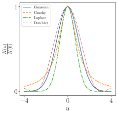
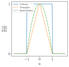
Figure 8: (left) Normalized non compactly-supported kernels; (right) normalized compactly-supported kernels detailed in Table 3.

Another natural choice consists in resorting to a divergence function $\phi$ such that $\kappa_{\rho}(\mathbf{z},\boldsymbol{\theta})\propto_{\mathbf{z}}\exp(-\rho^{-1}\phi(\mathbf{z},\boldsymbol{\theta}))$. Particular instances of these functions are the family of the Bregman divergences, which are ubiquitous tools in signal processing, machine learning and optimization (see Definition 1 of the main document). Table 4 recalls classical examples of Bregman divergences that can be used to define $\phi$. Again, only univariate examples of such potentials are provided but they can be easily extended to the multivariate case.

Table 4: Examples of divergence functions $\phi$ that can be used to define an appropriate density $\kappa_{\rho}$ verifying Property 1 in the main paper.

name	$\Theta$	$\phi(z,\theta)$
Squared loss	$\mathbb{R}$	$(z-\theta)^{2}$
Absolute loss	$\mathbb{R}$	$|z-\theta|$
Logistic loss	$[0,1]$	$z\log\left(\frac{z}{\theta}\right)+(1-z)\log\left(\frac{1-z}{1-\theta}\right)$
Itakura-Saito divergence	$\mathbb{R}_{+}$	$\frac{z}{\theta}-\log\left(\frac{z}{\theta}\right)-1$
Kullback-Leibler divergence	$[0,1]$	$z\log\left(\frac{z}{\theta}\right)$

Note that, reciprocally, tight connections have been already drawn between Bregman divergences and regular exponential family distributions. Indeed, when the function $\kappa_{\rho}$ belongs to the exponential family, its associated potential function defined by $-\log\kappa_{\rho}$ can be expressed as a Bregman divergence up to an additional term (Banerjee et al. 2005, Theorem 4)

$$-\log\kappa_{\rho}(\mathbf{z},\boldsymbol{\theta})=d_{\psi}(\mathbf{z},\mathbb{E}(\mathbf{z}|\boldsymbol{\theta}))-\log b_{\psi}(\mathbf{z}).$$ (124)

Appendix 3 Illustration for Lipschitz loss functions used in statistical learning

Some of the results of Section 4.3 in the main paper assume that the potential function $f$ associated to $\pi$ is Lipschitz. Interestingly, such Lipschitz functions are used in standard statistical learning problems to evaluate the discrepancy between observations and model outputs (van de Geer 2016).

Table 5: Lipschitz loss functions $f$ used in standard statistical learning problems. Their domain of definition is denoted $\mathcal{D}_{f}$ and $y$ stands for an observation. The notation “reg.” stands for regression.

name	problem	$\mathcal{D}_{f}$	$f(y;t)$
hinge	SVM	$\{-1,1\}\times\mathbb{R}$	$\max\left(0,1-yt\right)$
Huber	robust reg.	$\mathbb{R}\times\mathbb{R}$	$\left\{\begin{array}[]{l}(y-t)^{2}/(2\delta)\ \text{if}\ |y-t|\leq\delta\\ |y-t|-\delta/2\ \text{otherwise, where}\ \delta>0\end{array}\right.$
logistic	logistic reg.	$\{-1,1\}\times\mathbb{R}$	$\log(1+\exp(-yt))$
pinball	quantile reg.	$\mathbb{R}\times\mathbb{R}$	$\tau\max(0,t-y)+(1-\tau)\max(0,y-t)$, $\tau\in(0,1)$

Table 5 lists some of them along with their definition and associated statistical problems. Note that the absolute loss stands for a particular instance of the pinball loss with $\tau=0.5$. Figure 9 illustrates the form of these losses and associated regularized potentials $f_{\rho}$ with $\rho=1$ obtained via a Monte Carlo approximation.

Without loss of generality, these problems consider a likelihood function that can be written as in (32) in the main paper with

$$f_{j}(y_{j};\boldsymbol{\theta})=f(y_{j};\mathbf{x}_{j}^{T}\boldsymbol{\theta}),$$ (125)

where for $j\in[n]$, $\mathbf{x}_{j}$ is the feature vector associated with observation $y_{j}$; $f$ is one of the loss functions in Table 5 and $\boldsymbol{\theta}\in\mathbb{R}^{d}$ is the parameter to infer. Since all the loss functions listed in Table 5 are Lipschitz continuous w.r.t. their second argument $t$ with Lipschitz constant equal to 1, the potential $f_{j}$ in (125) is also Lipschitz with constant $L_{f_{j}}=\left\|\mathbf{x}_{j}\right\|_{2}$. Motivated by the robustness properties inherited by AXDA, see Section 3.3 in the main paper, we consider the smoothing of the likelihood contribution associated to each observation $f_{j}$ with a Gaussian kernel. The results of Corollary 3 in the main paper can then be applied to $\pi$ defined in (32) in the main paper.

In practice, to illustrate the behavior of the upper bound in Corollary 3 w.r.t. the number of observations, we fixed the dimension $d$ and considered several values of $n$ ranging from 1 to $10^{4}$. For each $n$, we randomly generated sets of features $\left\{\mathbf{x}_{j}\right\}_{j\in[n]}$ and we normalized the columns of the matrix $\mathbf{X}^{T}=\left[\mathbf{x}_{1},\ldots,\mathbf{x}_{n}\right]^{T}$ such that each entry is a random number between $0$ and $1$. The latter operation is classical in machine learning and is also called feature scaling.

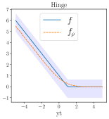
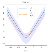
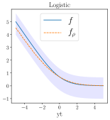
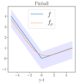
Figure 9: Loss functions of Table 5 along with their associated regularized loss $f_{\rho}$ with $\rho=1$ estimated with a Monte Carlo approximation. The Huber and pinball losses have been plotted with $\delta=1$ and $\tau=0.2$, respectively. The contours of the shaded area correspond to $f+L_{\rho}$ and $f+U_{\rho}$.

Figure 10 shows the behavior of the upper bound in Corollary 3 for two values of the dimension $d=10$ and $d=10^{3}$. As expected, the bound becomes less informative for a fixed value of $\rho$ as the number of likelihood approximations increases with the size of the dataset $n$. Nonetheless, the effect of $n$ on the bound is not highly prohibitive. In both cases $d=10$ and $d=10^{3}$, $\rho$ and $n$ appear to be complementary variables: increasing the value of the latter and decreasing the value of the former by the same factor roughly gives the same bound value. Actually, one can show that the dependence of the bound when $\rho$ is small is of the order $\mathcal{O}(n\rho)$ for a fixed dimension $d$, see the supplementary material. Obviously, one can limit this dependence on $n$ by splitting blocks of observations in minibatches instead of splitting each observation. This splitting strategy has for instance been considered by Rendell et al. (2020).

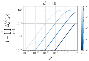
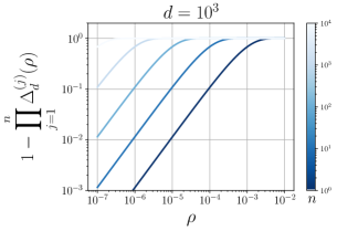
Figure 10: Behavior of the upper bound in Corollary 3 w.r.t. $\rho$ and $n$ for several values of the dimension $d$. The notation $\Delta^{(j)}_{d}(\rho)$ has been defined in Corollary 3.

Appendix 4 Inference details for the image inpainting example

In this section, we detail the steps of the Gibbs sampler used to sample from the posterior distribution $\pi_{\rho}(\boldsymbol{\theta},\mathbf{z}|\mathbf{y})$ in Section 5.4 in the main paper.

4.1 Sampling the auxiliary vector

The conditional distribution associated to the auxiliary variable $\mathbf{Z}=(\mathbf{z}_{1},\mathbf{z}_{2})$ writes

$$\pi_{\rho}(\mathbf{Z}|\boldsymbol{\theta})\propto \exp\left(-\tau\sum_{1\leq i\leq d}\left\|\mathbf{Z}_{i}\right\|_{2}-\dfrac{1}{2\rho^{2}}\left\|\mathbf{Z}-\mathbf{D}\boldsymbol{\theta}\right\|_{2}^{2}\right).$$ (126)

This conditional distribution can be sampled exactly by using data augmentation. Indeed, one can re-write the distribution involving the non-differentiable potential $\left\|\cdot\right\|_{2}$ as a mixture of normal and gamma distributions (Kyung et al. 2010, Section 3.1). Hence, sampling from (126) can be performed with the following two steps

$$\text{Draw }\dfrac{1}{\gamma_{i}}\sim\mathrm{InverseGaussian}\left(\dfrac{\tau}{\left\|\mathbf{Z}_{i}\right\|_{2}},\tau^{2}\right)\forall i\in[d],\text{ if $\left\|\mathbf{Z}_{i}\right\|_{2}>0$}$$

$$\text{Draw }\dfrac{1}{\gamma_{i}}\sim\mathrm{InverseGaussian}\left(\dfrac{3}{2},\dfrac{\tau^{2}}{2}\right)\forall i\in[d],\text{ if $\left\|\mathbf{Z}_{i}\right\|_{2}=0$}$$

$$\text{Draw }\mathbf{z}_{1,i}\sim\mathcal{N}\left(\dfrac{\gamma_{i}(D_{1}\boldsymbol{\theta})_{i}}{\rho^{2}+\gamma_{i}},\dfrac{\rho^{2}\gamma_{i}}{\rho^{2}+\gamma_{i}}\right)\forall i\in[d],$$

$$\text{Draw }\mathbf{z}_{2,i}\sim\mathcal{N}\left(\dfrac{\gamma_{i}(D_{2}\boldsymbol{\theta})_{i}}{\rho^{2}+\gamma_{i}},\dfrac{\rho^{2}\gamma_{i}}{\rho^{2}+\gamma_{i}}\right)\forall i\in[d].$$

Note that all these sampling steps can be performed efficiently by “vectorizing” them.

4.2 Sampling the parameter of interest

The conditional distribution associated to the image to recover $\boldsymbol{\theta}$ writes

$$\pi_{\rho}(\boldsymbol{\theta}|\mathbf{Z},\mathbf{y})\propto \exp\left(-\dfrac{1}{2\rho^{2}}\left\|\mathbf{Z}-\mathbf{D}\boldsymbol{\theta}\right\|_{2}^{2}-\dfrac{1}{2\sigma^{2}}\left\|\mathbf{y}-\mathbf{H}\boldsymbol{\theta}\right\|_{2}^{2}\right).$$ (127)

The distribution (127) is a non-degenerate Gaussian distribution $\mathcal{N}(\boldsymbol{\mu}_{\boldsymbol{\theta}},\mathbf{\Sigma}_{\boldsymbol{\theta}})$ where

$$\mathbf{\Sigma}_{\boldsymbol{\theta}} =\left(\rho^{-2}\mathbf{D}^{T}\mathbf{D}+\sigma^{-2}\mathbf{H}^{T}\mathbf{H}\right)^{-1}$$ (128)

$$\boldsymbol{\mu}_{\boldsymbol{\theta}} =\mathbf{\Sigma}_{\boldsymbol{\theta}}\left(\sigma^{-2}\mathbf{H}^{T}\mathbf{y}+\rho^{-2}\mathbf{D}^{T}\mathbf{Z}\right).$$ (129)

Sampling from this multivariate distribution can be done efficiently in $O(d\log d)$ floating point operations by resorting to the two-dimensional discrete Fourier transform. Indeed, under periodic boundary conditions for $\boldsymbol{\theta}$, the matrix $\mathbf{D}^{T}\mathbf{D}$ is a block circulant matrix and hence diagonalizable in the Fourier domain. On the other hand, $\mathbf{H}^{T}\mathbf{H}$ stands for a diagonal matrix with some zeros on the diagonal corresponding to the missing pixels. Since these two matrices cannot be diagonalized in the same domain, we use the auxiliary variable method of Marnissi et al. (2018) to decouple them. Let $\eta\left\|\mathbf{H}^{T}\mathbf{H}\right\|_{\mathrm{S}}<\sigma^{2}$ where $\left\|\mathbf{M}\right\|_{\mathrm{S}}$ is the spectral norm of the matrix $\mathbf{M}$. Then, we have the following two-step sampling scheme

$$\text{Draw }\mathbf{v}\sim\mathcal{N}\left(\left(\dfrac{\mathbf{I}_{d}}{\eta}-\dfrac{\mathbf{H}^{T}\mathbf{H}}{\sigma^{2}}\right)\boldsymbol{\theta},\dfrac{\mathbf{I}_{d}}{\eta}-\dfrac{\mathbf{H}^{T}\mathbf{H}}{\sigma^{2}}\right),$$

$$\text{Draw }\boldsymbol{\theta}\sim\mathcal{N}\left(\boldsymbol{\mu}_{\boldsymbol{\theta}},\mathbf{\Sigma}_{\boldsymbol{\theta}}\right),$$

where

$$\mathbf{\Sigma}_{\boldsymbol{\theta}}=\left(\dfrac{\mathbf{I}_{d}}{\eta}-\dfrac{\mathbf{D}^{T}\mathbf{D}}{\rho^{2}}\right)^{-1},$$

$$\boldsymbol{\mu}_{\boldsymbol{\theta}}=\mathbf{\Sigma}_{\boldsymbol{\theta}}\left(\mathbf{v}+\dfrac{\mathbf{H}^{T}}{\sigma^{2}}\mathbf{y}+\dfrac{\mathbf{D}^{T}}{\rho^{2}}\mathbf{Z}\right).$$

Appendix 5 Inference algorithms based on AXDA

Motivated by the issues detailed in Section 2, the good expected properties reviewed in Section 3 as well as the theoretical results shown in Section 4 in the main paper, this section shows that AXDA may allow to derive more efficient and distributed inference algorithms ranging from simulation to optimization-based methods. To do so, the potential benefits of AXDA in comparison with direct inference from $\pi$ are presented and discussed. MCMC and VB methods based on AXDA models are detailed to explore the distribution of the parameters to infer. Optimization-based approaches such as ADMM and the EM-algorithm are also derived if maximum likelihood (ML) or maximum a posteriori (MAP) estimates based on the approximate density $\pi_{\rho}$ are desired.

From now on, we assume that $\Theta=\mathbb{R}^{d}$ and we consider a target density with the general form

$$\pi(\boldsymbol{\theta})\propto\prod_{j=1}^{J}\pi_{j}(\mathbf{A}_{j}\boldsymbol{\theta})\propto\prod_{j=1}^{J}\displaystyle\exp\left(-f_{j}(\mathbf{A}_{j}\boldsymbol{\theta})\right).$$ (130)

Based on this target density, the augmented density $\pi_{\rho}$ is assumed to take the form

$$\pi_{\rho}(\boldsymbol{\theta},\mathbf{z}_{1\mathrel{\mathop{\mathchar 58\relax}}J})\propto\prod_{j=1}^{J}\pi_{j}(\mathbf{z}_{j})\kappa_{\rho}(\mathbf{z}_{j},\mathbf{A}_{j}\boldsymbol{\theta}).$$ (131)

This writing permits to highlight the benefits of using the augmented density $\pi_{\rho}$ instead of $\pi$ for each of the different inference approaches detailed in the sequel.

5.1 Monte Carlo sampling from AXDA

A standard way to sample from the joint density $\pi_{\rho}$ is to consider a Gibbs sampler as in Algorithm 1. This algorithm can make the inference tractable, simpler and/or faster by targetting $\pi_{\rho}$ instead of $\pi$. First, by splitting the initial potential $\sum_{j}f_{j}$, $\pi_{\rho}$ admits simpler and lower-dimensional conditional posterior distributions, each of them possibly defined by a single potential $f_{j}$. Within a Gibbs algorithm, these conditional posteriors yield simpler sampling steps, which may embed efficient dedicated state-of-the-art sampling methods. Second, given the current iterate $\boldsymbol{\theta}^{[t]}$, sampling each auxiliary variable $\mathbf{z}_{j}^{[t]}$ can be performed in an independent and parallel manner for a faster inference. This is of particular interest in big data settings where datasets are stored on multiple kernels or machines (Rendell et al. 2020). In addition, Vono et al. (2019) experimentally showed that considering AXDA-based models can even improve the convergence properties of classical MCMC methods such as Langevin Monte Carlo by embedding them. A detailed description of additional benefits of AXDA simulation-based methods and their illustration on image processing and machine learning problems can be found in Rendell et al. (2020) and Vono et al. (2019).

Input : Functions $f_{j}$, tolerance parameter $\rho$, initialization $\mathbf{z}^{[0]}$ and total nb. of iterations $T_{\mathrm{MC}}$

1 for $t\leftarrow 1$ to $T_{\mathrm{MC}}$ do

2      % Drawing the variable of interest $\boldsymbol{\theta}$

3       $\boldsymbol{\theta}^{[t]}\sim\pi_{\rho}(\boldsymbol{\theta}|\mathbf{z}^{[t-1]})=\displaystyle\prod_{j=1}^{J}\kappa_{\rho}(\mathbf{z}_{j}^{[t-1]},\mathbf{A}_{j}\boldsymbol{\theta})$;

4       % Drawing the splitting variables $\mathbf{z}_{j}$

5       for $j\leftarrow 1$ to $J$ do

6             $\mathbf{z}_{j}^{[t]}\sim\pi_{\rho}(\mathbf{z}_{j}|\boldsymbol{\theta}^{[t]})=\pi_{j}(\mathbf{z}_{j})\kappa_{\rho}(\mathbf{z}_{j},\mathbf{A}_{j}\boldsymbol{\theta}^{[t]})$;

7            

8       end for

9      

10 end for

Output : Collection of samples $\left\{\boldsymbol{\theta}^{[t]}\right\}_{t=1}^{T_{\mathrm{MC}}}$ asymptotically distributed according to $\pi_{\rho}$.

Algorithm 1 Gibbs sampler

Example 3.

We consider in this example the penalized logistic regression problem. We assume that $n$ binary responses $\mathbf{y}\in\{-1,1\}^{n}$ are observed and correspond to conditionally independent Bernoulli random variables with probability of success $\sigma(\mathbf{x}_{j}^{T}\boldsymbol{\theta})$. The function $\sigma$ is the sigmoid function, $\mathbf{x}_{j}\in\mathbb{R}^{d}$ stands for the feature vector associated to observation $y_{j}$ and $\boldsymbol{\theta}\in\mathbb{R}^{d}$ are the unknown regression coefficients to infer. We consider a zero-mean Gaussian prior distribution on $\boldsymbol{\theta}$ with precision $2\tau$, that is $g(\boldsymbol{\theta})=\tau\left\|\boldsymbol{\theta}\right\|_{2}^{2}$. The target $\pi$ then stands for the posterior distribution of the unknown regression coefficients $\boldsymbol{\theta}$

$$\pi(\boldsymbol{\theta}|\mathbf{y})\propto\displaystyle\exp\left(-g(\boldsymbol{\theta})-\sum_{j=1}^{n}\log\left[1+\exp\left(y_{j}\mathbf{x}_{j}^{T}\boldsymbol{\theta}\right)\right]\right).$$ (132)

By denoting $f_{(n+1)}=g$ and for all $j\in[n]$ with $J=n$, $f_{j}(u)=\log\left[1+\exp\left(y_{j}u\right)\right]$, the posterior distribution in (132) has the form (130) with $J=n+1$. Following the work of Polson et al. (2013), one can derive a promising DA scheme from $\pi$ based on the Polya-Gamma distribution. Hence, a Gibbs sampler can be used to sample from each conditional distribution as detailed by Polson et al. (2013). However, this Gibbs sampler scales poorly in high-dimensional settings as pointed out by Durmus and Moulines (2016). The AXDA alternative is Algorithm 1 with a quadratic potential and resulting conditional distributions

$$\pi_{\rho}(z_{j}|\boldsymbol{\theta},y_{j}) \propto\displaystyle\exp\left(-\log\left[1+\exp\left(y_{j}z_{j}\right)\right]-\dfrac{1}{\rho^{2}}(z_{j}-\mathbf{x}_{j}^{T}\boldsymbol{\theta})^{2}\right)\quad\forall j\in[n]$$ (133)

$$\pi_{\rho}(\boldsymbol{\theta}|\mathbf{z}_{1\mathrel{\mathop{\mathchar 58\relax}}n}) \propto\displaystyle\exp\left(-\tau\left\|\boldsymbol{\theta}\right\|_{2}^{2}-\sum_{j=1}^{n}\dfrac{1}{\rho^{2}}(z_{j}-\mathbf{x}_{j}^{T}\boldsymbol{\theta})^{2}\right).$$ (134)

Thanks to this splitting scheme, the inference is simpler, might be distributed, and sampling from these conditional distributions can be done exactly and efficiently. Indeed, since (133) is univariate and log-concave, one can use adaptive rejection sampling (Gilks and Wild 1992) while sampling the variable of interest $\boldsymbol{\theta}$ from (134) boils down to high-dimensional Gaussian sampling and efficient methods can be applied.

5.2 Variational Bayes inference from AXDA

AXDA can also be a major asset when conducting variational Bayes (VB) inference, providing important benefits such as simplicity and parallelization. VB methods (Bishop and Tipping 2000; Opper and Saad 2001) circumvent the direct sampling from a target density such as $\pi_{\rho}$ by defining an approximation of the latter denoted $\tilde{\pi}_{\rho}$. The best approximation is found by minimizing the Kullback-Leibler (KL) divergence between $\tilde{\pi}_{\rho}$ and $\pi_{\rho}$ restricted to a set of tractable candidates $\tilde{\pi}_{\rho}$. Depending on this set, a lot of VB approximation methods exist in the literature, see Bishop (2006) and Pereyra et al. (2016) for reviews. In this section, we will consider the widely-used mean-field approximation method where the approximate density $\tilde{\pi_{\rho}\text{}}$ is chosen among the set of conditionally independent (w.r.t. $\rho$) densities, that is $\tilde{\pi}_{\rho}(\boldsymbol{\theta},\mathbf{z}_{1\mathrel{\mathop{\mathchar 58\relax}}J})=\tilde{\pi}_{\rho}(\boldsymbol{\theta})\prod_{j=1}^{J}\tilde{\pi}_{\rho}(\mathbf{z}_{j})$. Under this constraint, the optimal choice of the VB approximation is given by

$$\log\tilde{\pi}_{\rho}(\boldsymbol{\theta})=\sum_{j=1}^{J}\mathbb{E}_{\tilde{\pi}_{\rho}(\mathbf{z}_{j})}\log\kappa_{\rho}(\mathbf{z}_{j},\mathbf{A}_{j}\boldsymbol{\theta})$$ (135)

$$\log\tilde{\pi}_{\rho}(\mathbf{z}_{j})=-f_{j}(\mathbf{z}_{j})+\mathbb{E}_{\tilde{\pi}_{\rho}(\boldsymbol{\theta})}\log\kappa_{\rho}(\mathbf{z}_{j},\mathbf{A}_{j}\boldsymbol{\theta}).$$ (136)

The above VB-marginals require to compute expectations under each marginal distribution which are often functions of moments under each marginal. Similarly to what has been encountered for Gibbs sampling in the previous section, deriving a VB approach based on $\pi_{\rho}$, instead of $\pi$, yields important benefits for parallel and possibly easier computations. Indeed, the VB-marginal in (136) shows again that each potential $f_{j}$ contributes independently given $\boldsymbol{\theta}$. The updates of expectations under (136) are thereby simplified since (i) the VB-marginals (136) are simpler than those obtained from a mean-field approximation of $\pi$ and (ii) the moments under the latter can be computed in parallel or distributed.

Example 3 (continued).

Jaakkola and Jordan (2000) considered a local VB algorithm for the penalized logistic regression problem. Instead of using a local VB approach and finding bounds on each individual function $f_{j}$, the use of $\pi_{\rho}$ instead of $\pi$ permits to consider directly a global VB approach such as the mean-field approximation. In addition, similarly to Algorithm 1, the updates of (136) and the associated expectations can be computed in parallel and efficiently by using state-of-the-art existing methods. For instance, the expectations $\mathbb{E}_{\tilde{\pi}_{\rho}(\mathbf{z}_{j})}$ can be approximated efficiently using rejection sampling.

5.3 Optimizing AXDA meets quadratic penalty methods

Computing the MAP or ML estimate under the AXDA model (131) boils down to solve the optimization problem

$$\min_{\boldsymbol{\theta},\mathbf{z}_{1\mathrel{\mathop{\mathchar 58\relax}}J}}\sum_{j=1}^{J}f_{j}(\mathbf{z}_{j})-\log\kappa_{\rho}(\mathbf{z}_{j},\mathbf{A}_{j}\boldsymbol{\theta}).$$ (137)

If $\kappa_{\rho}$ stands for a Gaussian kernel, the problem (137) can be viewed as a quadratically penalized formulation of the initial problem $\min_{\boldsymbol{\theta}}\sum_{j=1}^{J}f_{j}(\boldsymbol{\theta})$, see Nocedal and Wright (2006, Section 17.1). As expected, the solution of (137) stands for an approximate solution w.r.t. the initial optimization problem. The associated algorithm is depicted in Algorithm 2. Regarding this algorithm, one can clearly see the benefit of using a variable splitting approach as in AXDA: the initial potential is split into $J$ individual potentials with no operator acting on $\boldsymbol{\theta}$. Therefore, the corresponding minimization problems are simpler (e.g., associated proximity operators may become available) and can be handled in parallel.

We eventually point out that the benefits of Algorithm 2 highlighted previously are also shared with the ADMM (Boyd et al. 2011). Instead of solving the approximate optimization problem (137) which encodes the splitting operation with a quadratic regularization term, the latter builds on Lagrangian duality in order to provide an exact solution to the initial minimization problem $\min f_{j}$.

Input : Functions $f_{j}$, penalty parameter $\rho$, $t\leftarrow 0$ and $\mathbf{z}_{1\mathrel{\mathop{\mathchar 58\relax}}J}^{[0]}$

1 while stopping criterion not satisfied do

2      % Minimization w.r.t. $\boldsymbol{\theta}$

3       $\boldsymbol{\theta}^{[t]}\in\underset{\boldsymbol{\theta}}{\arg\min}\ \displaystyle\sum_{j=1}^{J}\dfrac{1}{2\rho^{2}}\left\|\mathbf{A}_{j}\boldsymbol{\theta}-\mathbf{z}_{j}^{[t-1]}\right\|_{2}^{2}$;

4       for $j\leftarrow 1$ to $J$ do

5             % Minimization w.r.t. $\mathbf{z}_{j}$

6             $\mathbf{z}_{j}^{[t]}\in\underset{\mathbf{z}_{j}}{\arg\min}\ f_{j}(\mathbf{z}_{j})+\dfrac{1}{2\rho^{2}}\left\|\mathbf{A}_{j}\boldsymbol{\theta}^{[t]}-\mathbf{z}_{j}\right\|_{2}^{2}$;

7            

8       end for

9      % Updating iterations counter

10       $t\leftarrow t+1$ ;

11      

12 end while

Output : MAP or ML estimate depending on the considered problem.

Algorithm 2 Quadratic penalty minimization

Example 3 (continued).

Computing directly the MAP estimate with classical forward-backward algorithms (e.g., the fast iterative shrinkage-thresholding algorithm (FISTA) (Beck and Teboulle 2009)) associated to $\pi$ is challenging if the observations are distributed among multiple nodes. In addition, proximity operators associated to $f_{j}$ are generally not available in closed-form because of the operators $\mathbf{A}_{j}$. Algorithm 2 permits to tackle these issues by splitting the initial objective function. In particular, the minimization w.r.t. $\mathbf{z}_{j}$ for $j\in[J]$ corresponds to an unidimensional $l_{2}$ regularized logistic regression problem that can be dealt with gradient-based methods with few iterations. The minimization w.r.t. $\boldsymbol{\theta}$ boils down to the solving of a linear system where efficient solvers can be applied. Note that such a splitting scheme avoids the use of stochastic gradient methods.

5.4 Expectation-maximization for AXDA

An EM algorithm under the augmented density $\pi_{\rho}(\boldsymbol{\theta},\mathbf{z})$ will target the MAP or ML estimator, see Algorithm 3. If the expectations in the E-step cannot be evaluated, one can use a Monte Carlo approximation to approximate them (Wei and Tanner 1990). The benefits of using the augmented density $\pi_{\rho}$ instead of $\pi$ are threefolds. Firstly, as pointed out in Section 2 in the main paper, exact DA schemes based on $\pi$ cannot be derived in general cases and corresponding EM algorithms cannot be implemented. Instead, considering $\pi_{\rho}$ gives a quite systematic way of introducing latent variables in the original statistical model. Secondly, the expectations involved in the E-step of Algorithm 3 can be simpler to derive than the expectation under $\pi$. Indeed, the latter involves the whole potential $\sum_{j}f_{j}$ while the former involves regularized parts $f_{j}-\log\kappa_{\rho}$ of this potential separately. Finally, conditionally on $\boldsymbol{\theta}^{[t]}$, the random variables $\mathbf{z}_{j}$ are independent. Thus, each expectation involved in the E-step can be computed in parallel.

Input : Functions $f_{j}$, penalty parameter $\rho$, $t\leftarrow 0$ and $\boldsymbol{\theta}^{[0]}$

1 while stopping criterion not satisfied do

2      % E-step

3       Define $Q(\boldsymbol{\theta}|\boldsymbol{\theta}^{[t]})=\displaystyle\sum_{j=1}^{J}\mathbb{E}_{\pi_{\rho}(\mathbf{z}_{j}|\boldsymbol{\theta}^{[t]})}\left(-f_{j}(\mathbf{z}_{j})+\log\kappa_{\rho}(\mathbf{z}_{j},\mathbf{A}_{j}\boldsymbol{\theta})\right)$;

4       % M-step

5      ; Compute $\boldsymbol{\theta}^{[t+1]}=\underset{\boldsymbol{\theta}}{\arg\max}\ Q(\boldsymbol{\theta}|\boldsymbol{\theta}^{[t]})$;

6       % Updating iterations counter

7       $t\leftarrow t+1$ ;

8      

9 end while

Output : MAP or ML estimate depending on the considered problem.

Algorithm 3 EM

Example 3 (continued).

Again, following the work of Polson et al. (2013), if the potential $g$ of the prior distribution is quadratic or corresponds to a sparsity-promoting $\ell_{p}$-penalization ($0<p\leq 1$), a simple EM-algorithm can be derived as detailed by Scott and Sun (2013). However, although this EM algorithm can be generalized to an online version, it does not scale to distributed and high-dimensional problems. On the other hand, the E-step of Algorithm 3 can be processed in parallel by computing the $J$ expectations on individual nodes: thanks to the AXDA approach, the algorithm is therefore suited to distributed and high-dimensional scenarios.

References

• Aguirregabiria et al. (2002) Aguirregabiria, J. M., Hernández, A., and Rivas, M. (2002), “$\delta$-function converging sequences,” American Journal of Physics, 70, 180–185.
• Albert and Chib (1993) Albert, J. H. and Chib, S. (1993), “Bayesian Analysis of Binary and Polychotomous Response Data,” Journal of the American Statistical Association, 88, 669–679.
• Ambrosio et al. (2008) Ambrosio, L., Gigli, N., and Savaré, G. (2008), Gradient flows in metric spaces and in the space of probability measures, Lectures in Mathematics. ETH Zürich, Birkhäuser Verlag, 2nd ed.
• Banerjee et al. (2005) Banerjee, A., Merugu, S., Dhillon, I. S., and Ghosh, J. (2005), “Clustering with Bregman Divergences,” Journal of Machine Learning Research, 6, 1705–1749.
• Baragatti et al. (2013) Baragatti, M., Grimaud, A., and Pommeret, D. (2013), “Likelihood-free parallel tempering,” Statistics and Computing, 23, 535–549.
• Barbos et al. (2017) Barbos, A.-C., Caron, F., Giovannelli, J.-F., and Doucet, A. (2017), “Clone MCMC: parallel high-dimensional Gaussian Gibbs sampling,” in Advances in Neural Information Processing Systems, pp. 5020–5028.
• Beaumont et al. (2002) Beaumont, M. A., Zhang, W., and Balding, D. J. (2002), “Approximate Bayesian Computation in Population Genetics,” Genetics, 162, 2025–2035.
• Beck and Teboulle (2009) Beck, A. and Teboulle, M. (2009), “A Fast Iterative Shrinkage-Thresholding Algorithm for Linear Inverse Problems,” SIAM Journal on Imaging Sciences, 2, 183–202.
• Ben-Tal et al. (2001) Ben-Tal, A., Margalit, T., and Nemirovski, A. (2001), “The Ordered Subsets Mirror Descent Optimization Method with Applications to Tomography,” SIAM Journal on Optimization, 12, 79–108.
• Besag and Green (1993) Besag, J. and Green, P. J. (1993), “Spatial Statistics and Bayesian Computation,” Journal of the Royal Statistical Society, Series B, 55, 25–37.
• Bishop (2006) Bishop, C. M. (2006), Pattern Recognition and Machine Learning, Springer-Verlag.
• Bishop and Tipping (2000) Bishop, C. M. and Tipping, M. E. (2000), “Variational Relevance Vector Machines,” in Conference on Uncertainty in Artificial Intelligence.
• Bolte et al. (2014) Bolte, J., Sabach, S., and Teboulle, M. (2014), “Proximal alternating linearized minimization for nonconvex and nonsmooth problems,” Mathematical Programming, 146, 459–494.
• Boyd et al. (2011) Boyd, S., Parikh, N., Chu, E., Peleato, B., and Eckstein, J. (2011), “Distributed Optimization and Statistical Learning via the Alternating Direction Method of Multipliers,” Foundations and Trends in Machine Learning, 3, 1–122.
• Bredies et al. (2010) Bredies, K., Kunisch, K., and Pock, T. (2010), “Total Generalized Variation,” SIAM Journal on Imaging Sciences, 3, 492–526.
• Canny (2004) Canny, J. (2004), “GaP: A Factor Model for Discrete Data,” in Annual International ACM SIGIR Conference on Research and Development in Information Retrieval, pp. 122–129.
• Chambolle (2004) Chambolle, A. (2004), “An Algorithm for Total Variation Minimization and Applications,” Journal of Mathematical Imaging and Vision, 20, 89–97.
• Chambolle et al. (2010) Chambolle, A., Novaga, M., Cremers, D., and Pock, T. (2010), “An introduction to total variation for image analysis,” in Theoretical Foundations and Numerical Methods for Sparse Recovery, De Gruyter.
• Choi and Hobert (2013) Choi, H. M. and Hobert, J. P. (2013), “The Pólya-Gamma Gibbs sampler for Bayesian logistic regression is uniformly ergodic,” Electronic Journal of Statistics, 7, 2054–2064.
• Combettes and Pesquet (2011) Combettes, P. L. and Pesquet, J.-C. (2011), “Proximal Splitting Methods in Signal Processing,” in Fixed-Point Algorithms for Inverse Problems in Science and Engineering, eds. Bauschke, H. H., Burachik, R., Combettes, P., Elser, V., Luke, D., and Wolkowicz, H., Springer, pp. 185–212.
• Damien et al. (1999) Damien, P., Wakefield, J., and Walker, S. (1999), “Gibbs sampling for Bayesian non-conjugate and hierarchical models by using auxiliary variables,” Journal of the Royal Statistical Society, Series B, 61, 331–344.
• Dang and Ehrhardt (2012) Dang, Q. A. and Ehrhardt, M. (2012), “On Dirac delta sequences and their generating functions,” Applied Mathematics Letters, 25, 2385 – 2390.
• Del Moral et al. (2012) Del Moral, P., Doucet, A., and Jasra, A. (2012), “An adaptive sequential Monte Carlo method for approximate Bayesian computation,” Statistics and Computing, 22, 1009–1020.
• Dempster et al. (1977) Dempster, A. P., Laird, N. M., and Rubin, D. B. (1977), “Maximum Likelihood from Incomplete Data via the EM Algorithm,” Journal of the Royal Statistical Society, Series B, 39, 1–38.
• Dharmadhikari and Joag-Dev (1988) Dharmadhikari, S. and Joag-Dev, K. (1988), Unimodality, Convexity, and Applications, New York: Academic Press.
• Dobson and Barnett (2008) Dobson, A. J. and Barnett, A. G. (2008), An Introduction to Generalized Linear Models, Texts in Statistical Science, Boca Raton, FL: Chapman & Hall/CRC Press, 3rd ed.
• Doucet et al. (2002) Doucet, A., Godsill, S. J., and Robert, C. P. (2002), “Marginal maximum a posteriori estimation using Markov chain Monte Carlo,” Statistics and Computing, 12, 77–84.
• Duane et al. (1987) Duane, S., Kennedy, A., Pendleton, B. J., and Roweth, D. (1987), “Hybrid Monte Carlo,” Physics Letters B, 195, 216–222.
• Dümbgen and Rufibach (2009) Dümbgen, L. and Rufibach, K. (2009), “Maximum likelihood estimation of a log-concave density and its distribution function: Basic properties and uniform consistency,” Bernoulli, 15, 40–68.
• Durmus and Moulines (2016) Durmus, A. and Moulines, E. (2016), “High-dimensional Bayesian inference via the Unadjusted Langevin Algorithm,” [online]. Technical report. Available at https://arxiv.org/abs/1605.01559/.
• Durmus and Moulines (2017) — (2017), “Nonasymptotic convergence analysis for the unadjusted Langevin algorithm,” The Annals of Applied Probability, 27, 1551–1587.
• Durmus et al. (2018) Durmus, A., Moulines, E., and Pereyra, M. (2018), “Efficient Bayesian Computation by Proximal Markov chain Monte Carlo: When Langevin Meets Moreau,” SIAM Journal on Imaging Sciences, 11, 473–506.
• Edwards and Sokal (1988) Edwards, R. G. and Sokal, A. D. (1988), “Generalization of the Fortuin-Kasteleyn-Swendsen-Wang representation and Monte Carlo algorithm,” Physical Review D, 38, 2009–2012.
• Fearnhead and Prangle (2012) Fearnhead, P. and Prangle, D. (2012), “Constructing summary statistics for approximate Bayesian computation: semi-automatic approximate Bayesian computation,” Journal of the Royal Statistical Society, Series B, 74, 419–474.
• Fellows et al. (2019) Fellows, M., Mahajan, A., Rudner, T. G. J., and Whiteson, S. (2019), “VIREL: A Variational Inference Framework for Reinforcement Learning,” in Advances in Neural Information Processing Systems, pp. 7120–7134.
• Folland (1999) Folland, G. (1999), Real Analysis: Modern Techniques and their Applications, New York: Wiley, 2nd ed.
• Geman and Reynolds (1992) Geman, D. and Reynolds, G. (1992), “Constrained restoration and the recovery of discontinuities,” IEEE Transactions on Pattern Analysis and Machine Intelligence, 14, 367–383.
• Geman and Yang (1995) Geman, D. and Yang, C. (1995), “Nonlinear image recovery with half-quadratic regularization,” IEEE Transactions on Image Processing, 4, 932–946.
• Gilks and Wild (1992) Gilks, W. R. and Wild, P. (1992), “Adaptive Rejection Sampling for Gibbs Sampling,” Journal of the Royal Statistical Society. Series C (Applied Statistics), 41, 337–348.
• Giovannelli (2008) Giovannelli, J. F. (2008), “Unsupervised Bayesian Convex Deconvolution Based on a Field With an Explicit Partition Function,” IEEE Transactions on Image Processing, 17, 16–26.
• Gradshteyn and Ryzhik (2015) Gradshteyn, I. S. and Ryzhik, I. M. (2015), Table of Integrals, Series, and Products, London: Academic Press, 8th ed.
• Hartley (1958) Hartley, H. O. (1958), “Maximum Likelihood Estimation from Incomplete Data,” Biometrics, 14, 174–194.
• Higdon (2007) Higdon, D. (2007), A Primer on Space-Time Modeling from a Bayesian Perspective, Chapman & Hall/CRC, pp. 217–279.
• Higdon (1998) Higdon, D. M. (1998), “Auxiliary Variable Methods for Markov Chain Monte Carlo with Applications,” Journal of the American Statistical Association, 93, 585–595.
• Holmes and Mallick (2003) Holmes, C. C. and Mallick, B. K. (2003), “Generalized Nonlinear Modeling With Multivariate Free-Knot Regression Splines,” Journal of the American Statistical Association, 98, 352–368.
• Hurn (1997) Hurn, M. (1997), “Difficulties in the use of auxiliary variables in Markov chain Monte Carlo methods,” Statistics and Computing, 7, 35–44.