Projected site-occupation embedding theory

Abstract

Site-occupation embedding theory (SOET) [B. Senjean et al., Phys. Rev. B 97, 235105 (2018)] is an in-principle exact embedding method combining wavefunction theory and density functional theory that gave promising results when applied to the one-dimensional Hubbard model. Despite its overall good performance, SOET faces a computational cost problem as its auxiliary impurity-interacting system remains the size of the full system (which is problematic as the computational cost increases exponentially with system size). In this work, this issue is circumvented by employing the Schmidt decomposition, thus leading to a drastic reduction of the computational cost while retaining the same accuracy. We show that this projected version of SOET (P-SOET) is competitive with other embedding techniques such as density matrix embedding theory (DMET) [G. Knizia and G. K-L. Chan, Phys. Rev. Lett. 109, 186404 (2012)]. In contrast to the latter, density functional contributions come naturally into play in P-SOET’s framework without any additional computational cost or double counting effect. As an important result, the density-driven Mott–Hubbard transition in one dimension (which is displayed by multiple impurity sites in DMET or in dynamical mean-field theory) is well described, for the first time, with a single impurity site.

I Introduction

Due to their unusual and remarkable properties, strongly correlated materials play an important role in the development of innovative technologies, such as photovoltaic cells, pharmaceuticals and industrial catalysts. These developments would greatly benefit from an accurate theoretical description. Unfortunately, the infamous exponential wall problem prevents the use of correlated wavefunction methods, and alternatives must be considered. A major milestone has been delivered by Kohn-Sham density functional theory (KS-DFT) Hohenberg and Kohn (1964); Kohn and Sham (1965). Despite its in-principle exact mathematical foundation, strongly correlated systems still remain challenging for the present density functional approximations Cohen et al. (2011); Swart (2013); Swart and Gruden (2016). Alternatively, quantum embedding theories Sun and Chan (2016) have been proposed and are the main focus of this paper. The strategy of embedding techniques consists in solving only a small part of the system (referred to as the fragment) by a high-level method, while a low-level approximation is used for the rest of the system (referred to as the environment). Green-function-based methods have been developed, such as the widely used dynamical mean-field theory (DMFT) Georges and Kotliar (1992); Georges et al. (1996); Kotliar and Vollhardt (2004); Kotliar et al. (2006); Held (2007); Vollhardt et al. (2012); Martin et al. (2016) or the more recent self-energy embedding theory (SEET) Kananenka et al. (2015); Lan et al. (2015, 2016); Zgid and Gull (2017); Lan et al. (2017); Tran et al. (2018); Rusakov et al. (2018). If one is interested about ground-state properties only, the Green function can be replaced by frequency-independent variables, such as the one-particle reduced density matrix (1RDM) or the electron density. This has led to the density matrix embedding theory (DMET) Knizia and Chan (2012), the density embedding theory (DET) Bulik et al. (2014), and related methods that allow overlapping between fragments Welborn et al. (2016); Ricke et al. (2017); Ye et al. (2018); Mordovina et al. (2019). They rely on the Schmidt decomposition of the full system wavefunction. It generates an embedded problem sufficiently small to be solved by exact diagonalization Knizia and Chan (2012, 2013); Bulik et al. (2014), density matrix renormalization group Wouters et al. (2016), auxiliary-field quantum Monte Carlo Zheng et al. (2017a) and more recently the complete active space self-consistent field Pham et al. (2018); Hermes and Gagliardi (2019). In practice, the exact wavefunction of the full system is not known and has been approximated by Hartree–Fock (HF) Knizia and Chan (2012, 2013), spin-unrestricted HF Bulik et al. (2014), HF-Bogoliubov LeBlanc et al. (2015); Zheng and Chan (2016), antisymmetrized geminal power Tsuchimochi et al. (2015), block-product states for spin lattices Fan and Jie (2015); Gunst et al. (2017), multiconfigurational self-consistent field Hermes and Gagliardi (2019) and KS-DFT Mordovina et al. (2019). Note that DMET has been mostly applied to model Hamiltonians Knizia and Chan (2012); Bulik et al. (2014); LeBlanc et al. (2015); Tsuchimochi et al. (2015); Zheng and Chan (2016); Zheng et al. (2017a, b); Fan and Jie (2015); Gunst et al. (2017); Sandhoefer and Chan (2016); Reinhard et al. (2019); Mukherjee and Reichman (2017) but also to quantum chemical systems Knizia and Chan (2013); Wouters et al. (2016); Pham et al. (2018); Hermes and Gagliardi (2019). Extension to excited-state properties Chen et al. (2014); Booth and Chan (2015) and to non-equilibrium electron dynamics Kretchmer and Chan (2018) have been investigated, as well as rigorous combinations of DMET with DMFT Fertitta and Booth (2018) and with the rotational invariant slave bosons theory Lee et al. (2019a).

In this work, a new method stemming from site-occupation embedding theory (SOET) Fromager (2015); Senjean et al. (2017, 2018a, 2018b); Senjean (2018) is proposed and relies on the Schmidt decomposition. In SOET, only the fragment is explicitly interacting, in the line of DMET (in its non-interacting bath formulation) and other embedding approaches. But instead of being approximated, the environment is described in-principle exactly by a complementary functional of the density. Still in its early stages, SOET has been applied to the one-dimensional Hubbard model although an extension to quantum chemistry is not excluded Fromager (2015); Senjean (2018). The attractiveness of SOET resides in its in-principle exact embedding framework that combines both wavefunction theory (WFT) and DFT without double counting problem. However, it has remained prohibitively expensive, as the size of the auxiliary impurity-interacting system remained the size of the original (fully-interacting) problem. In this work, we take advantage of the Schmidt decomposition to rigorously remove most of the degrees of freedom in the environment, and to replace it by a bath that is the same size as the fragment (i.e. the impurity-interacting sites). We refer to this new method as projected-SOET (P-SOET), and apply it to the one-dimensional uniform Hubbard model up to 400 sites. We show that P-SOET yields accurate results at a drastically reduced computational cost.

The paper is organized as follows. After a brief summary of the key equations of SOET in Sec. II.1, P-SOET and its implementation are introduced in Sec. II.2. Details on the functionals of the density are given in Sec. II.3 followed by the computational details in Sec. III. Results obtained on the one-dimensional uniform Hubbard model are provided in Sec. IV. The density-driven Mott-transition is studied in Sec. IV.4. Finally, conclusions and perspectives are given in Sec. V.

II Theory

II.1 Site-occupation embedding theory

For the paper to be self-contained, this section summarizes the key equations of SOET Fromager (2015); Senjean et al. (2017, 2018a, 2018b). We start with the (not necessarily uniform) one-dimensional $L$-site Hubbard model in an external potential ($\mathbf{v}\equiv\{v_{i}\}_{i}$),

$$\hat{H}=-t\sum_{i=0,\sigma}^{L-1}\left(\hat{c}_{i\sigma}^{\dagger}\hat{c}_{i+1\sigma}+h.c.\right)+U\sum_{i=0}^{L-1}\hat{n}_{i\uparrow}\hat{n}_{i\downarrow}+\sum_{i=0}^{L-1}v_{i}\hat{n}_{i},$$

with $t>0$ the hopping parameter between first neighbor sites and $U$ the on-site electronic repulsion. The site-occupation operator $\hat{n}_{i}=\hat{n}_{i\uparrow}+\hat{n}_{i\downarrow}$ (with $\hat{n}_{i\sigma}=\hat{c}_{i\sigma}^{\dagger}\hat{c}_{i\sigma}$) is expressed using the creation ($\hat{c}_{i\sigma}^{\dagger}$) and annihilation ($\hat{c}_{i\sigma}$) operators of an electron of spin $\sigma$ on site $i$. The ground-state energy of this model can be expressed in site-occupation functional theory (SOFT) Gunnarsson and Schönhammer (1986); Schönhammer et al. (1995) (DFT analog for model Hamiltonians) using the following variational principle:

$$E(\mathbf{v})=\underset{\mathbf{n}}{\rm min}\left\{F(\mathbf{n})+(\mathbf{v}|\mathbf{n})\right\},$$ (2)

where

$$F(\mathbf{n})=\underset{\Psi\rightarrow\mathbf{n}}{\rm min}\left\{\left\langle\Psi\middle|\hat{T}+\hat{U}\middle|\Psi\right\rangle\right\}$$ (3)

is the Levy-Lieb (LL) functional and $(\mathbf{v}|\mathbf{n})=\sum_{i}v_{i}n_{i}$. The idea of SOET relies on mapping the fully interacting problem onto a partially interacting one. The interacting sites are referred to as impurities, and $M$ impurities are embedded in a bath of $(L-M)$ noninteracting sites. (Note that the term bath in SOET actually refers to the environment in DMET.) This is done by decomposing the conventional LL functional as follows Senjean et al. (2018b):

$$F(\mathbf{n})=F_{M}^{\rm imp}(\mathbf{n})+\overline{E}_{{\rm Hxc},M}^{\rm bath}(\mathbf{n}),$$ (4)

where

$$F_{M}^{{\rm imp}}(\mathbf{n})=\underset{\Psi\rightarrow\mathbf{n}}{\rm min}\left\{\left\langle\Psi\middle|\hat{T}+\hat{U}_{M}\middle|\Psi\right\rangle\right\}$$ (5)

is the $M$-impurity-interacting functional with $\hat{U}_{M}=U\sum^{M-1}_{i=0}\hat{n}_{i\uparrow}\hat{n}_{i\downarrow}$, and $\overline{E}_{{\rm Hxc},M}^{\rm bath}(\mathbf{n})$ is the complementary Hxc bath energy, functional of the sites occupation. Inserting this decomposition into Eq. (2) leads to the variational principle within SOET Senjean et al. (2018b):

$$E(\mathbf{v})=\underset{\Psi}{\rm min}\Big{\{} \left\langle\Psi\middle|\hat{T}+\hat{U}_{M}\middle|\Psi\right\rangle+\overline{E}_{{\rm Hxc},M}^{\rm bath}\left(\mathbf{n}^{\Psi}\right)+\left(\mathbf{v}|\mathbf{n}^{\Psi}\right)\Big{\}},$$

where $\mathbf{n}^{\Psi}\equiv\left\{\langle\Psi|\hat{n}_{i}|\Psi\rangle\right\}_{i}$. The minimizing $M$-impurity-interacting wavefunction $\Psi_{M}^{\rm imp}$ in Eq. (II.1) reproduces the exact density profile of the fully-interacting system and fulfills the following self-consistent equation:

$$\left(-t\sum_{i=0,\sigma}^{L-1}\left(\hat{c}_{i\sigma}^{\dagger}\hat{c}_{i+1\sigma}+{\rm H.c.}\right)+\hat{U}_{M}+\displaystyle\sum_{i=0}^{L-1}v_{M,i}^{\rm emb}\hat{n}_{i}\right)|\Psi_{M}^{\rm imp}\rangle$$ (7)

$$=\mathcal{E}_{M}^{\rm imp}|\Psi_{M}^{\rm imp}\rangle,$$

where $\mathcal{E}^{\rm imp}_{M}$ is the impurity auxiliary energy (i.e., the ground-state energy of the $M$-impurity interacting Hamiltonian) and

$$v^{\rm emb}_{M,i}=v_{i}+\dfrac{\partial\overline{E}^{\rm bath}_{{\rm Hxc},M}(\mathbf{n}^{\Psi^{\rm imp}_{M}})}{\partial n_{i}}$$ (8)

corresponds to the embedding potential for the $M$ impurities embedded into the $(L-M)$ bath sites. Concerning the complementary Hxc bath functional, it can be shown that Fromager (2015)

$$\overline{E}_{{\rm c},M}^{\rm bath}(\mathbf{n})=E_{\rm c}(\mathbf{n})-E_{{\rm c},M}^{\rm imp}(\mathbf{n}),$$ (9)

where $E^{\rm imp}_{{\rm c},M}(\mathbf{n})$ is the analog of the correlation functional for the $M$-impurity-interacting system. Turning to the uniform problem investigated in this paper [$\mathbf{v}=0$ in Eq. (II.1)], the local density approximation (LDA) of $E_{\rm c}(\mathbf{n})$ is exact and reads

$$E_{\rm c}(\mathbf{n})=\sum_{i}e_{\rm c}(n_{i}),$$ (10)

where $e_{\rm c}(n)$ is the per-site correlation energy functional. In addition, the exact per-site energy $e=E(\mathbf{v}=\mathbf{0})/L$ and double occupation expressions for the uniform Hubbard model have been derived in Ref. Senjean et al. (2018b) and read

$$e = \dfrac{1}{M}\left.\sum^{M-1}_{i=0}\left[t_{\rm s}(n_{i}^{\Psi})+t\dfrac{\partial e_{\rm c}(n_{i}^{\Psi})}{\partial t}+{U}\langle\hat{n}_{i\uparrow}\hat{n}_{i\downarrow}\rangle_{\Psi}\right]\right|_{\Psi=\Psi_{M}^{\rm imp}}$$ (11)

$$+\left.U\dfrac{\partial\overline{e}_{{\rm c},M}^{\rm bath}({\bf n}^{\Psi})}{\partial U}\right|_{\Psi={\Psi_{M}^{\rm imp}}},$$

and

$$d=\dfrac{1}{M}\sum^{M-1}_{i=0}\langle\hat{n}_{i\uparrow}\hat{n}_{i\downarrow}\rangle_{\Psi_{M}^{\rm imp}}+\dfrac{\partial\overline{e}_{{\rm c},M}^{\rm bath}({\bf n}^{\Psi_{M}^{\rm imp}})}{\partial U},$$ (12)

respectively, where $t_{s}(n)=-4t\sin(\pi n/2)/\pi$ is the (one-dimensional) per-site non-interacting kinetic energy functional and

$$\overline{e}_{{\rm c},M}^{\rm bath}(\mathbf{n})=\dfrac{1}{M}\left[\left(\sum^{M-1}_{i=0}e_{c}(n_{i})\right)-E_{{\rm c},M}^{\rm imp}(\mathbf{n})\right]$$ (13)

is the per-site analog of the bath correlation energy in Eq. (9). Interestingly, the per-site energy and the double occupation are related to each other as follows:

$$e = Ud+\dfrac{1}{M}\left.\sum^{M-1}_{i=0}\left[t_{\rm s}(n_{i}^{\Psi})+t\dfrac{\partial e_{\rm c}(n_{i}^{\Psi})}{\partial t}\right]\right|_{\Psi={\Psi_{M}^{\rm imp}}}.$$ (14)

II.2 Projected site-occupation embedding theory

In SOET, the auxiliary impurity-interacting problem has the same size as the full system even though the interactions are restricted to the fragment of interest. This is the actual bottleneck of SOET. Indeed, as currently implemented, considering the kinetic operator in the whole system in Eq. (7) does not lead to any reduction of the computational cost compared to solving the fully-interacting system. In the following, we describe how the Schmidt decomposition is employed in P-SOET to drastically reduce the size of the system to which a correlated wavefunction theory is applied. First, we review the Schmidt decomposition introduced by Knizia and Chan within the now well-established DMET Knizia and Chan (2012). We then discuss how to derive the embedded problem in P-SOET.

II.2.1 Review of the Schmidt decomposition

Suppose that the system is divided into a fragment $F$ and the rest of the system (referred to as the “environment”) $E$. For instance, regarding the SOET Hamiltonian in Eq. (7), the fragment is composed of the $M$ explicitly interacting impurity sites while the remaining implicitly interacting sites correspond to the environment. Note that in SOET, the latter is referred to as the bath, but in this paper we will follow the DMET nomenclature where the bath states are obtained after the Schmidt decomposition. The total Hilbert space of the system is the tensor product of $F$ and $E$, $\mathcal{H}=\mathcal{H}_{F}\otimes\mathcal{H}_{E}$, where $\mathcal{H}_{F}$ ($\mathcal{H}_{E}$) has size $N_{F}=d^{L_{F}}$ ($N_{E}=d^{L_{E}}$). $L_{F}$ ($L_{E}$) is the number of sites in subsystem $F$ ($E$). Given that a site is equivalent to a spatial orbital, there are $d=4$ possible occupations: empty, singly occupied with spin-projection $s^{z}=\pm 1/2$, and doubly occupied $\{|0\rangle,|\uparrow\rangle,|\downarrow\rangle,|\uparrow\downarrow\rangle\}$. Let $\{|F_{i}\rangle\}_{i}$ ($\{|E_{j}\rangle\}_{j}$) denote the many-body basis of size $N_{F}$ ($N_{E}$). $\mathcal{H}$ is then spanned by $N_{F}N_{E}=4^{L_{F}+L_{E}}=4^{L}$ many-body states denoted by $\{|F_{i}\rangle|E_{j}\rangle\}_{ij}$. The ground state in $\mathcal{H}$ can be expressed as

$$|\Psi_{0}\rangle=\sum_{i=1}^{N_{F}}\sum_{j=1}^{N_{E}}C_{ij}|F_{i}\rangle|E_{j}\rangle.$$ (15)

Performing the singular value decomposition and assuming $N_{F}<N_{E}$ leads to

$$|\Psi_{0}\rangle = \sum_{i=1}^{N_{F}}\sum_{j=1}^{N_{E}}\sum_{n=1}^{N_{F}}U_{in}\lambda_{n}V^{\dagger}_{nj}|F_{i}\rangle|E_{j}\rangle$$ (16)

$$= \sum_{n=1}^{N_{F}}\lambda_{n}|\tilde{F}_{n}\rangle|\tilde{B}_{n}\rangle,$$

where $U_{in}$ and $V_{jn}^{*}=V_{nj}^{\dagger}$ rotate the many-body basis $\{|F_{i}\rangle\}_{i}$ and $\{|E_{j}\rangle\}_{j}$ into a new many-body basis $\{|\tilde{F}_{n}\rangle\}_{n}$ and $\{|\tilde{B}_{n}\rangle\}_{n}$ (where $\tilde{B}$ now refers to the new bath states, to be distinguished with the environment states). Eq. (16) is called the Schmidt decomposition of the wavefunction Knizia and Chan (2012), now expressed within the reduced Hilbert space spanned by $N_{F}^{2}=4^{2L_{F}}$ many-body states (denoted by $\{|\tilde{F}_{m}\rangle|\tilde{B}_{n}\rangle\}_{mn}$), thus removing most of the degrees of freedom in the environment. The corresponding embedded Hamiltonian is then obtained by projection,

$$\hat{H}^{\rm emb}=P^{\dagger}\hat{H}P,$$ (17)

where $P$ defines the projector onto the Schmidt basis,

$$P=\sum_{m=1,n=1}^{N_{F}}|\tilde{F}_{m}\rangle|\tilde{B}_{n}\rangle\langle\tilde{B}_{n}|\langle\tilde{F}_{m}|.$$ (18)

This projector does not affect the exact ground-state wavefunction, $P|\Psi_{0}\rangle=|\Psi_{0}\rangle$, such that

$$\hat{H}|\Psi_{0}\rangle=E_{0}|\Psi_{0}\rangle\rightarrow\hat{H}^{\rm emb}|\Psi_{0}\rangle=E_{0}|\Psi_{0}\rangle.$$ (19)

The ground state of the embedded Hamiltonian is then also the ground state of the full system. However, this exact decomposition requires the a priori knowledge of the exact wavefunction, which is of course not known. An approximate wavefunction has to be used instead and the single Slater determinant obtained from a KS-SOFT calculation is considered in this work, thus leading to approximate single-particle bath states $|\tilde{B}_{n}\rangle$.

II.2.2 P-SOET

Let us consider the fully-interacting lattice problem given by the $L$-site uniform Hubbard Hamiltonian. The first step is to obtain the approximate single-particle bath states defining the projection operator from a non-interacting system as reference. In DMET, this reference commonly corresponds to the mean-field approximation of the physical system. In P-SOET, it makes sense to consider a non-interacting system which has the same density as the physical one, as this density will be used in the determination of the per-site energy and the double occupation [Eqs. (11) and (12)]. Hence, we consider the KS-SOFT Hamiltonian,

$$\hat{h}^{\rm KS}=-t\sum_{i=0,\sigma}^{L-1}\left(\hat{c}_{i\sigma}^{\dagger}\hat{c}_{i+1\sigma}+{\rm H.c.}\right)+\sum_{i=0}^{L-1}\dfrac{\partial E_{\rm Hxc}(\mathbf{n})}{\partial n_{i}}\hat{n}_{i},$$

because its (self-consistently determined) effective potential reproduces the same density as the physical system, in principle exactly. Note that this choice has also been made recently by Mordovina et al. Mordovina et al. (2019). The obtained density is then inserted into Eq. (8) to determine the analytical embedding potential, used to construct the one-body effective Hamiltonian

$$\hat{h}^{\rm eff}=-t\sum_{i=0,\sigma}^{L-1}\left(\hat{c}_{i\sigma}^{\dagger}\hat{c}_{i+1\sigma}+{\rm H.c.}\right)+\sum_{i=0}^{L-1}v_{M,i}^{\rm emb}\hat{n}_{i},$$

which is nothing but the one-body part of the SOET Hamiltonian in Eq. (7) ($\hat{H}^{\rm SOET}=\hat{h}^{\rm eff}+\hat{U}_{M}$).

The one-body part of the embedded Hamiltonian is then obtained by projecting the one-body effective Hamiltonian [Eq. (II.2.2)] as follows:

$$\hat{h}^{\rm emb}=P^{\dagger}\hat{h}^{\rm eff}P,$$ (22)

where the projector $P$ [of size $(L\times 2L_{F})$] comes from the Schmidt decomposition of the ground state $\Phi_{\rm KS}$ of $\hat{h}^{\rm KS}$  and reads Ayral et al. (2017)

$$P=\begin{bmatrix}\mathbbm{1}&0\\ 0&C_{B}C_{F}^{\dagger}\end{bmatrix}.$$ (23)

$\mathbbm{1}$ denotes the identity matrix of size $(L_{F}\times L_{F})$ and $C_{B}C_{F}^{\dagger}$ is a $(L_{E}\times L_{F})$ rectangular matrix which is the transformation from the environment to the bath. The reader is referred to Ref. Ayral et al. (2017) for a detailed construction of this projector. As readily seen in Eq. (23), the transformation of the one-particle fragment states in the original basis is the identity. The fragment is therefore invariant under this projection. The on-site electron repulsion is then added to the fragment (or impurity) sites thus leading to the following many-body embedded Hamiltonian:

$$\hat{H}^{\rm emb}=\sum_{ij}^{L_{F}+L_{B}}h^{\rm emb}_{ij}\left(\hat{c}_{i\sigma}^{\dagger}\hat{c}_{j\sigma}+{\rm H.c.}\right)+U\sum_{i}^{L_{F}}\hat{n}_{i\uparrow}\hat{n}_{i\downarrow},$$

where $L_{F}$ (equivalent to $M$ introduced previously) and $L_{B}$ are the number of fragment sites and bath sites, respectively, and $L_{F}=L_{B}$. We refer to $\Psi^{\rm emb}_{M}$ as its associated ground-state wavefunction. The closed embedded subsystem (fragment+bath) is then twice the size of the fragment and consists of $4L_{F}$ spin-orbitals (or $2L_{F}$ sites) with $2L_{F}$ electrons. One can therefore see the fragment as being an open system with the bath playing the role of a reservoir, i.e. the fragment can contain a fractional number of electrons Knizia and Chan (2013). This is a drastic simplification of SOET as well as an alternative to DMET where the correlation potential is now functional of the density. From $\Psi^{\rm emb}_{M}$, we extract the impurity double occupations

$$\langle\hat{n}_{i\uparrow}\hat{n}_{i\downarrow}\rangle_{\Psi^{\rm emb}_{M}},\leavevmode\nobreak\ \leavevmode\nobreak\ 0\leqslant i\leqslant M-1.$$ (25)

Together with the KS-SOFT density, they are used to determine the physical per-site energy and double occupation in Eqs. (11) and (12), respectively. Another significant difference with DMET is that no matching condition (known to be a bottleneck of DMET Wu et al. (2019)) between the 1RDM of the low-level and the high-level wavefunctions is requested in P-SOET. Instead, only the in-principle exact density (from the low-level KS determinant) is determined self-consistently, while the high-level embedded wavefunction together with complementary functionals of the density allows for an accurate evaluation of physical observables. Note that one can determine the density of the impurity sites

$$n_{i}^{\Psi^{\rm emb}_{M}}=\langle\hat{n}_{i\uparrow}+\hat{n}_{i\downarrow}\rangle_{\Psi^{\rm emb}_{M}},\leavevmode\nobreak\ \leavevmode\nobreak\ 0\leqslant i\leqslant M-1$$ (26)

self-consistently, and use it instead of the KS-SOFT density. For the sake of conciseness, this alternative procedure is described in Appendix B.

The procedure detailed in this section can be summarized as follows:

1. Solve the KS-SOFT problem [Eq. (II.2.2)]

2. Apply the Schmidt decomposition to the KS determinant and determine the projection operator $P$

3. Determine the one-body effective Hamiltonian [Eq. (II.2.2)] with the density obtained from Step 1

4. Project the effective Hamiltonian to obtain the one-body embedded Hamiltonian [Eq. (22)]

5. Define the embedded Hamiltonian by adding interaction on the fragment sites [Eq. (II.2.2)]

6. Solve the embedded problem to get the embedded wavefunction $\Psi^{\rm emb}_{M}$

These steps define the P-SOET algorithm, pictured in Fig. 1 for a single impurity site.

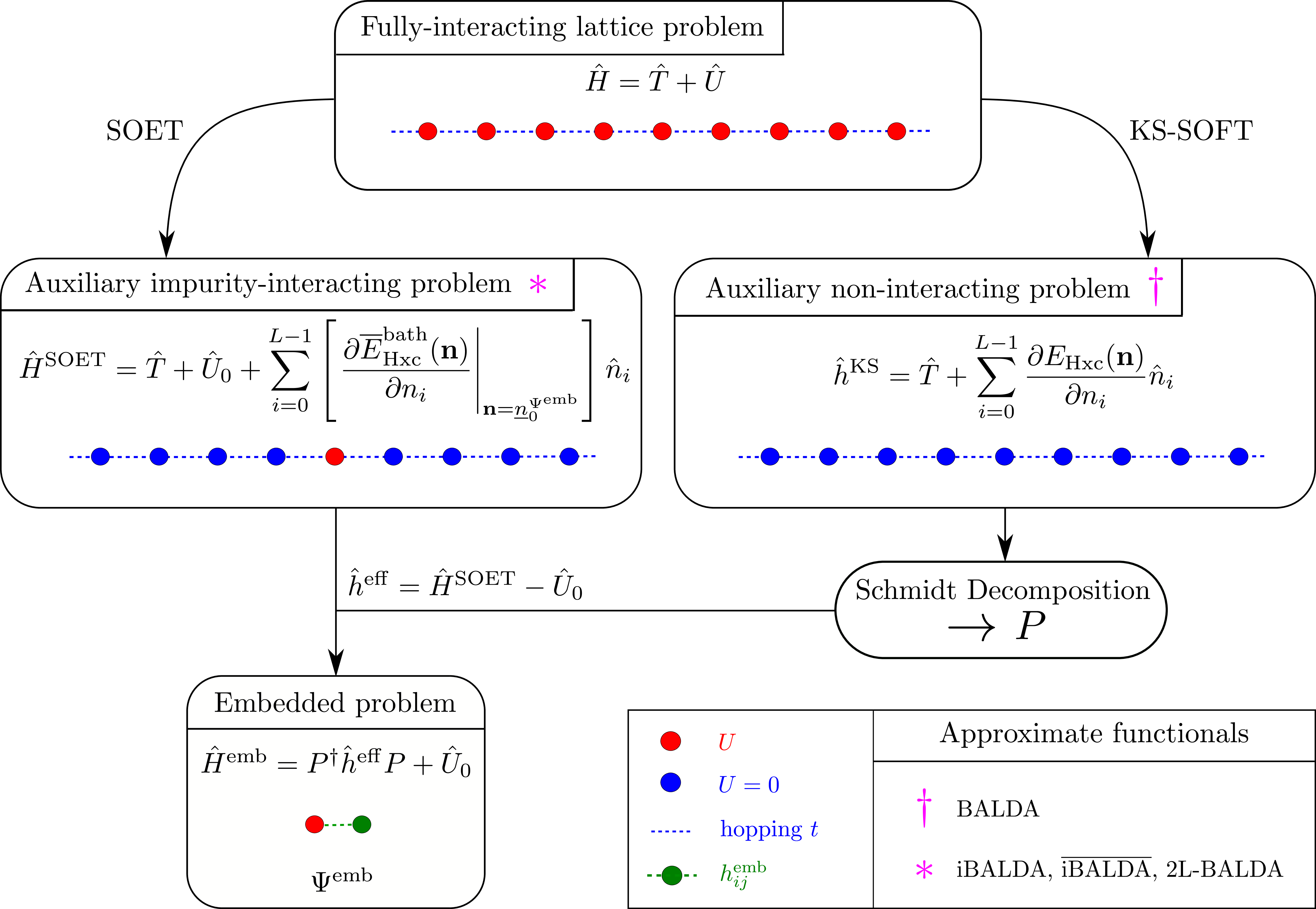
Figure 1: Representation of the P-SOET algorithm for a single impurity site. In SOET, the auxiliary impurity-interacting problem has to be solved entirely. In P-SOET, it is projected onto a much smaller embedded problem thanks to the Schmidt decomposition of the auxiliary non-interacting problem. An optional self-consistent loop can be added to update the impurity occupation obtained by solving the embedded problem (see Appendix. B and Fig. 9).

II.3 Approximate functionals

The performance of SOET and P-SOET relies on the accuracy of the per-site correlation functional $e_{\rm c}(n)$ and the impurity correlation functional $E_{{\rm c},M}^{\rm imp}(\mathbf{n})$, as well as their derivatives with respect to $U$, $t$ and $n_{i}$ Senjean et al. (2018b). The LDA based on Bethe Ansatz (BA) (so-called BALDA) is used for $e_{\rm c}(n)$ Lima et al. (2002, 2003); Capelle et al. (2003), and is exact in the thermodynamic limit for $U=0$, $U\rightarrow+\infty$ and $n=1$ for any $U$. For the impurity correlation functional, a two-level (2L) approximation based on the Anderson dimer has been derived in Ref. Senjean et al. (2017). Together with BALDA, it leads to the so-called 2L-BALDA functional Senjean et al. (2018b), which can be used in the single-impurity case only. Alternatively, one can use BALDA for the impurity functional as well. This simple approximation enables us to consider more impurities and is called the $M$-impurity BALDA [iBALDA($M$)] Senjean et al. (2018b). By construction [see Eq. (13)], $\overline{e}_{{\rm c},M}^{\rm bath}(\mathbf{n})$ and its derivatives are equal to 0 within iBALDA($M$). The reader is referred to Ref. Senjean et al. (2018b) for more details on these functionals and their derivations.

In SOET, the exact embedding potential for a finite and half-filled ($\mathbf{n}=\underline{1}$) system,

$$v^{\rm emb}_{M,i}(\mathbf{n}=\underline{1})=-\dfrac{U}{2}\sum_{j=0}^{M-1}\delta_{ij},$$ (27)

has always been used Senjean et al. (2018a, b). While Eq. (27) is always fulfilled by the 2L-BALDA functional, it is not by iBALDA. Indeed, iBALDA has been derived from the thermodynamic limit ($L\rightarrow+\infty$), for which a derivative discontinuity in the correlation energy functional appears at half-filling Lima et al. (2002); Capelle et al. (2003); Senjean et al. (2018a) such that the correlation potential is not defined anymore. Eq. (27) has then been enforced in previous works. In this work, another choice is made. The BALDA (or equivalently, iBALDA) correlation potential Lima et al. (2002, 2003); Capelle et al. (2003),

$$\dfrac{\partial e_{\rm c}^{\rm BALDA}(n<1)}{\partial n} = -2t\cos\left(\dfrac{\pi n}{\beta(U/t)}\right)+2t\cos\left(\dfrac{\pi n}{2}\right)$$ (28)

$$-\dfrac{Un}{2},$$

will take the following value at half-filling,

$$\dfrac{\partial e_{\rm c}^{\rm BALDA}(n=1)}{\partial n} = \left.\dfrac{\partial e_{\rm c}^{\rm BALDA}(n<1)}{\partial n}\right|_{n=1^{-}}$$ (29)

$$= -2t\cos\left(\dfrac{\pi}{\beta(U/t)}\right)-\dfrac{U}{2}.$$

[Rather than being equal to 0 to fulfill Eq. (27).] This choice makes the embedding potential smooth in the range $0\leqslant n\leqslant 1$, instead of $0\leqslant n<1$. We refer to this new functional with an overbar: $\overline{\rm iBALDA}$. The change between $\overline{\rm iBALDA}$ and iBALDA operates only at half-filling and is made clear by representing the correlation potential in Fig. 2. Note that in contrast to iBALDA, the 2L-BALDA correlation potential depicts no discontinuity at half-filling (Fig. 9 of Ref. Senjean et al. (2018b)).

Why haven’t we made this choice previously ? In SOET, convergence issues may arise around half-filling when either the impurity or the bath occupations come very close to 1. These issues appear in iBALDA if the BALDA correlation potential [Eq. (29)] were used to solve the self-consistent SOET equation. This problem is due to the presence of the Mott metal-insulator transition at half-filling, and also arises in KS-SOFT (for inhomogeneous systems with BALDA) Lima et al. (2003). In P-SOET, the situation is different. The density is determined self-consistently from a KS-SOFT calculation (which is always exact for a uniform system), while the embedded problem is solved only once. Therefore, Eq. (29) can be used at half-filling in P-SOET without leading to any convergence issue. We show in Sec. IV that choosing the $\overline{\rm iBALDA}$ embedding potential at half-filling instead of the iBALDA one improves the results drastically, although the resulting impurity occupation is not exact anymore. (In any case, the exact KS-SOFT occupations are used to compute the per-site energy and the double occupation in P-SOET.)

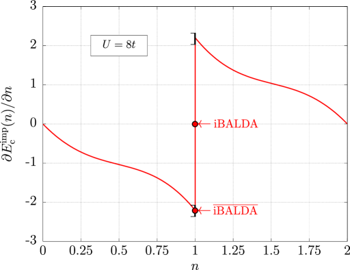
Figure 2: BALDA correlation potential with respect to $n$ for $U=8t$. At half-filling ($n=1$), the iBALDA impurity correlation potential is exact for a finite system and is equal to 0, while the $\overline{\rm iBALDA}$ impurity correlation potential is not and is given by Eq. (29).

III Computational details

Three main calculations are performed in P-SOET: ($i$) the KS-SOFT calculation of the physical problem to get $\Phi_{\rm KS}$ [Eq. (II.2.2)], ($ii$) the Schmidt decomposition of $\Phi_{\rm KS}$ and ($iii$) solving the embedded problem [Eq. (II.2.2)]. As the uniform one-dimensional Hubbard model is studied in this paper, the first step simply consists in a mean-field calculation with no potential. Indeed, the KS potential is defined up to a constant, and is also uniform for a uniform system. The second step follows the implementation detailed in Ref. Ayral et al. (2017). Finally, the embedded problem is solved either analytically for a single impurity site (see Appendix A) or numerically for multiple impurities by using the Block code of density matrix renormalization group (DMRG) Chan and Head-Gordon (2002); Chan (2004); Ghosh et al. (2008); Sharma and Chan (2012); Olivares-Amaya et al. (2015). The derivations of the SOET functionals can be found in Ref. Senjean et al. (2018b), and are implemented in the source code for P-SOET which is freely available Senjean . In this work, the $L$-site uniform one-dimensional Hubbard model is studied with an even number $N$ of electrons. Periodic ($\hat{c}_{L\sigma}=\hat{c}_{0\sigma}$) and antiperiodic ($\hat{c}_{L\sigma}=-\hat{c}_{0\sigma}$) boundary conditions have been used when $(N/2)\leavevmode\nobreak\ {\rm mod}\leavevmode\nobreak\ 2=1$ (i.e., $N/2$ is an odd number) and $(N/2)\leavevmode\nobreak\ {\rm mod}\leavevmode\nobreak\ 2=0$ (i.e., $N/2$ is an even number), respectively. Results are compared to the exact BA results Lieb and Wu (1968); Shiba (1972); Lieb and Wu (2003). $L=400$ sites are considered in this work and the hopping parameter has been set to $t=1$ in all the calculations.

IV Results

After evaluating the errors coming from the projection (constructed from approximate single-particle bath states) onto the impurity model subspace, the per-site energy [Eq. (11)] and the double occupation [Eq. (12)] are calculated within P-SOET as described in Sec. II.2. The focus will be first on the half-filled case, followed by the hole-doping regime. Finally, the density-driven Mott–Hubbard transition is investigated and found to be properly described by P-SOET with a single impurity site, in contrast to DMET Knizia and Chan (2012); Bulik et al. (2014) and DMFT Capone et al. (2004) for which multiple impurities are required.

IV.1 Errors due to the projection

Because the projector is expressed in terms of approximate single-particle states, P-SOET is no more in-principle exact in contrast to SOET (providing that exact functionals are used). It is therefore essential to evaluate the errors due to this projection, in addition to those introduced in the functionals. Such an analysis is performed by comparing the impurity occupation and double occupation within SOET and P-SOET using the exact SOET embedding potential, obtained by reverse engineering Senjean et al. (2017) on the uniform $L=12$ sites Hubbard model with a single impurity site. By construction, the impurity occupation obtained in SOET by using this potential is the exact one Senjean et al. (2017). However, the one obtained after projection is not exact anymore except in the particular case of half-filling, as shown in Table 1. As readily seen in Table 1, the impurity occupation in P-SOET deviates from the exact occupation as $U/t$ increases. Nevertheless the error remains relatively low, of the order of $10^{-2}$.

	$N=2$	$N=4$	$N=6$	$N=8$	$N=10$	$N=12$
Exact	0.16667	0.33333	0.5	0.66667	0.83333	1
$U=t$	0.16559	0.33174	0.49883	0.66618	0.83329	1
$U=2t$	0.16377	0.32854	0.49613	0.66488	0.83305	1
$U=3t$	0.16209	0.32520	0.49296	0.66307	0.83251	1
$U=4t$	0.16068	0.32223	0.48990	0.66104	0.83167	1
$U=5t$	0.15954	0.31972	0.48719	0.65904	0.83057	1
$U=6t$	0.15861	0.31765	0.48489	0.65718	0.82930	1
$U=7t$	0.15784	0.31593	0.48296	0.65553	0.82796	1
$U=8t$	0.15720	0.31449	0.48134	0.65409	0.82663	1
$U=9t$	0.15666	0.31327	0.47997	0.65284	0.82537	1
$U=10t$	0.15621	0.31224	0.47881	0.65177	0.82421	1
$U=100t\leavevmode\nobreak\ \leavevmode\nobreak\ \leavevmode\nobreak\ \leavevmode\nobreak\ \leavevmode\nobreak\$	0.15141	0.30184	0.46785	0.63440	0.81267	1

Table 1: Impurity occupation obtained by solving the embedded problem in P-SOET. The exact SOET embedding potential for a uniform $L=12$ sites Hubbard model with one impurity site has been used.

Turning to the impurity double occupation, let us consider the half-filled case where the exact potential does indeed lead to the exact impurity occupation, even in P-SOET. In Fig. 3, the impurity double occupation is shown for both SOET and P-SOET with respect to $U/(U+4t)$. Note that the range $0\leqslant U/(U+4t)\leqslant 1$ covers the entire correlation regime, from the weakly correlated one $U<4t$ [$U/(U+4t)<1/2$], to the strongly correlated one $U>4t$ [$U/(U+4t)>1/2$]. The noninteracting and atomic limits are given by $U=0$ [$U/(U+4t)=0$] and $t=0$ [$U/(U+4t)=1$], respectively. We observe a very small change between the impurity double occupations in Fig. 3, and conclude that the projection does not lead to substantial errors. Therefore, the errors will almost entirely be due to the use of approximate functionals.

The iBALDA and 2L-BALDA results within P-SOET are then not expected to differ much from the ones obtained with SOET in Ref. Senjean et al. (2018b), and are mostly plotted for comparison with the novel $\overline{\rm iBALDA}(M)$ approximation introduced in Sec. II.3.

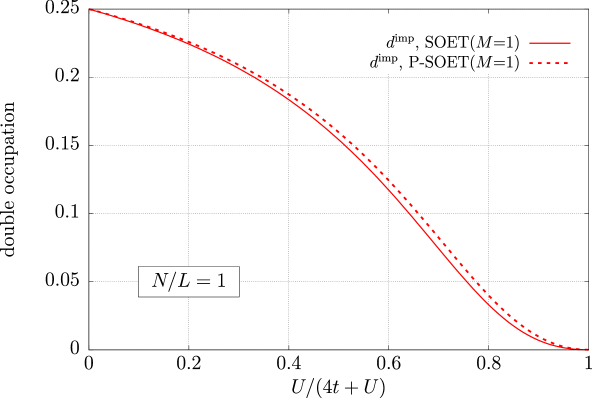
Figure 3: Impurity double occupation $d^{\rm imp}=\langle\hat{n}_{0\uparrow}\hat{n}_{0\downarrow}\rangle_{\Psi_{M}}$ as a function of correlation strength. The wavefunction $\Psi_{M}$ is obtained by solving the SOET Hamiltonian [Eq. (7)] ($\Psi^{\rm imp}_{M}$, full lines), and the embedded problem in P-SOET [Eq. (II.2.2)] ($\Psi^{\rm emb}_{M}$, dashed lines). The uniform and half-filled Hubbard model with $L=12$ and a single impurity site is considered. In both cases, the exact embedding potential in Eq. (27) has been used.

IV.2 Half-filled case

Let us first focus on the half-filled Hubbard model, known to be a Mott insulator for any $U>0$. Fig. 4 shows the per-site energy obtained within P-SOET for different approximations. First of all, all the approximations are exact in the noninteracting and atomic limits. As already discussed in Ref. Senjean et al. (2018b), it is clear that the iBALDA($M$=1) is not accurate enough at half-filling due to the absence of bath correlation functional, above all in the moderate and strong correlation regimes. Considering a non-zero bath correlation functional like in 2L-BALDA improves over iBALDA($M$=1). With a single impurity site, 2L-BALDA gives similar results than iBALDA($M$=4) in the weak and moderate correlation regime but is less accurate in the strongly correlated one. Still considering a single impurity, $\overline{\rm iBALDA}$($M$=1) is surprisingly significantly more accurate than iBALDA($M$=1) and 2L-BALDA for $U\geqslant 4t$. By increasing the number of impurities, $\overline{\rm iBALDA}$($M$=4) is now almost on top of the exact BA per-site energy. In comparison with DMET (Fig. 2 of Ref. Bulik et al. (2014)), $\overline{\rm iBALDA}$ gives a better per-site energy than the so-called “NI”, and is even competitive with the so-called “NI_F”, which are nothing but the noninteracting bath formulations of DMET where the matching condition is performed on the 1RDM of the fragment and on the full 1RDM of the fragment+bath, respectively Bulik et al. (2014). We refer the reader to Ref. Bulik et al. (2014) for more details about those two versions of DMET.

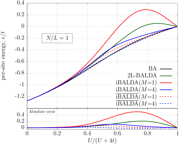
Figure 4: Per-site energy [Eq. (11)] as a function of correlation strength for different approximations in P-SOET. The uniform and half-filled $L=400$ site Hubbard is considered. The absolute error with respect to BA is plotted in the bottom panel.

Let us now turn to the double occupation in Fig. 5. As expected, the double occupation within iBALDA and 2L-BALDA are similar to the one obtained in SOET Senjean et al. (2018b), demonstrating again that errors due to the projection are negligible. Interestingly, the double occupation obtained within iBALDA($M$=1) is identical to the one of DMET for a single impurity site Knizia and Chan (2012); Bulik et al. (2014). This can be explained as follows: for a single impurity site at half-filling the iBALDA embedding potential returns the exact density, exactly like the numerically optimized correlation potential of DMET. Therefore, we see no reason why the embedded wavefunction of both theories should be different in this case, thus leading to the same impurity double occupation. However, the method overestimates the exact double occupation. Just like the per-site energy, 2L-BALDA improves over iBALDA($M$=1) in the entire correlation regime. An even better double occupation is obtained with iBALDA($M$=4) especially in the strongly correlated regime, but this is at the expense of a much higher computational cost. Indeed, a single impurity can be solved analytically (see Appendix A) while four impurities require to solve a fragment+bath system of eight sites (or 16 spin orbitals) and eight electrons with a high-level wavefunction method. Turning to $\overline{\rm iBALDA}$($M$=1), the double occupation is worse than iBALDA($M$=1) for $U\leqslant 1.8t$, but becomes rapidly more accurate than 2L-BALDA or even iBALDA($M$=4). With four impurity sites, $\overline{\rm iBALDA}$($M$=4) is also not highly accurate in the very weakly correlated regime, but tends towards the exact double occupation otherwise.

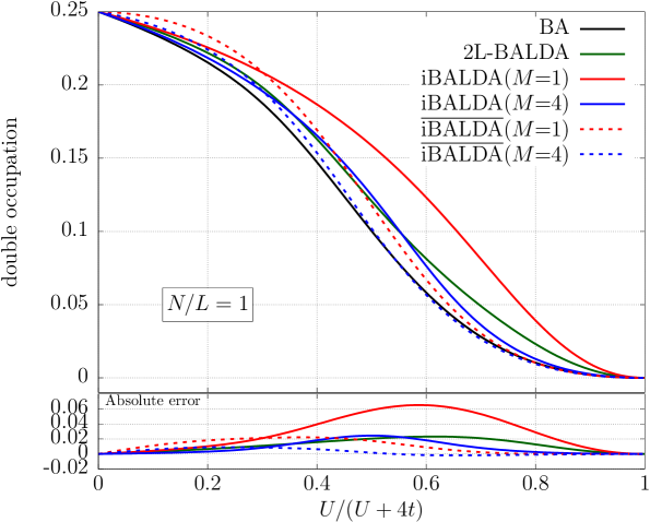
Figure 5: Double occupation [Eq. (12)] as a function of correlation strength for different approximations in P-SOET. The uniform and half-filled $L=400$ site Hubbard is considered. The absolute error with respect to BA is plotted in the bottom panel.

Finally, the fact that the bare (i.e. without density functional contributions) impurity double occupation changes that much between iBALDA and $\overline{\rm iBALDA}$ means that the embedding potential has a strong influence on the embedded wavefunction. Although the embedding potential in $\overline{\rm iBALDA}$ is no more exact at half-filling for a finite system and does not lead to the exact density (as discussed in Sec. II.3), it may take into account the so-called exchange-correlation derivative-discontinuity responsible for the description of the Mott insulator. This derivative-discontinuity has been discussed by Capelle et al. for the BALDA functional Lima et al. (2002); Capelle et al. (2003) and in Ref. Senjean et al. (2018a) for SOET functionals. This could explain why $\overline{\rm iBALDA}$ is the most accurate approximation at half-filling (in the moderate and strong correlation regimes).

IV.3 Hole-doped regime

Let us now investigate the hole-doped region ($0.4\leqslant N/L\leqslant 1$) of the uniform Hubbard model for moderate ($U=4t$) and strong ($U=8t$) correlation strengths. Note that in previous works Senjean et al. (2018a, b), we were limited to $L=32$ sites for computational cost reason. Within P-SOET, $L=400$ sites is easily tractable as the most costly part now consists in solving an embedded problem of 2$L_{F}$ sites only. As a consequence, we can get closer to the thermodynamic limit. Because iBALDA and $\overline{\rm iBALDA}$ differ at half-filling only, they will give exactly the same result in the density domain $0.4\leqslant N/L<1$. To have smooth potentials in the range $0.4\leqslant N/L\leqslant 1$, $\overline{\rm iBALDA}$ is used instead of iBALDA (see Fig. 2).

In the case of $U=4t$ (top panel of Fig. 6), 2L-BALDA and $\overline{\rm iBALDA}$($M$=1) are already fairly accurate and almost indistinguishable from each other. Nevertheless, they both tends to overestimate the per-site energy closer they get to half-filling. Increasing the number of impurities reduces the error considerably, and $\overline{\rm iBALDA}$($M$=4) becomes almost exact for $N/L\geqslant 0.7$. For stronger correlation strength (bottom panel of Fig. 6), $\overline{\rm iBALDA}$($M$=1) is now much more accurate. By comparison with Fig. 3 of Ref. Bulik et al. (2014), the single-impurity $\overline{\rm iBALDA}$($M$=1) gives a better per-site energy than NI and NI_F with two impurities. It is even comparable to DET and DMET in the broken spin symmetry formalism, also with two impurities Bulik et al. (2014). 2L-BALDA still overestimates the per-site energy close to half-filling, while $\overline{\rm iBALDA}$($M$=4) is again almost exact.

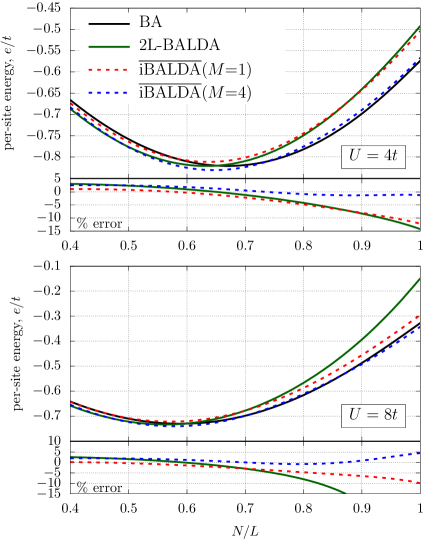
Figure 6: Per-site energy as a function of the density filling for different approximations in P-SOET. The $L=400$ sites Hubbard model with $U=4t$ (top panel) and $U=8t$ (bottom panel) is considered. The relative error with respect to BA is plotted in the bottom of each panel.

Turning to the double occupation in Fig. 7, one can see that the bare impurity double occupation $d^{\rm imp}$ obtained with 2L-BALDA overestimates the exact double occupation considerably around half-filling. The physical double occupation within 2L-BALDA is more accurate as expected. The analysis of Fig. 7 is then similar to Fig. 6, due to the relation between the double occupation and the per-site energy [Eq. (14)]. (The term in square brackets in Eq. (14) is approximated by BALDA, which is accurate in all regimes except the very weakly correlated one Senjean et al. (2018a), not studied here). Therefore the double occupation within $\overline{\rm iBALDA}$($M$=1) is also very accurate, especially for $U=8t$. Increasing the number of impurities does improve the result slightly, but might not be worth it here considering its higher computational cost.

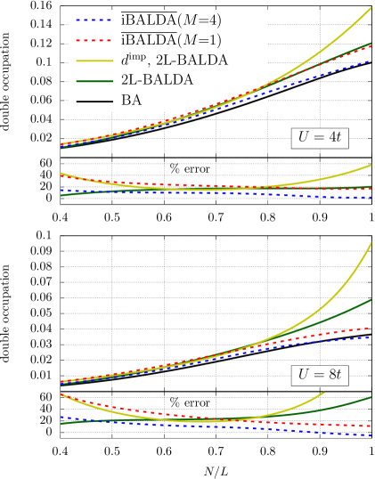
Figure 7: Double occupation as a function of the density filling for different approximations in P-SOET. The $L=400$ sites Hubbard model with $U=4t$ (top panel) and $U=8t$ (bottom panel) is considered. The relative error with respect to BA is plotted in the bottom of each panel.

IV.4 Density-driven Mott–Hubbard transition

The most interesting behavior of the one-dimensional Hubbard model is certainly the paramagnetic density-driven Mott–Hubbard transition. In one dimension, the Hubbard model describes a paramagnetic metallic state, except at half-filling where it becomes a paramagnetic Mott-insulator (for any $U>0$) manifested by the opening of a charge gap. Therefore, a density-driven Mott metal-insulator transition arises when passing from the infinitesimally hole-doped case ($N/L=1-\delta$, with $\delta$ infinitesimal and strictly positive) to the half-filled case ($N/L=1$). Such a transition, which is not a result of antiferromagnetism, is detected by vanishing compressibility (or charge susceptibility $\partial N(\mu)/\partial\mu$) Knizia and Chan (2012). It can be observed by plotting $N(\mu)$ with respect to $\mu$, where $N(\mu)$ is the electron number associated with the chemical potential $\mu$ and is obtained by minimizing the grand canonical energy of the following Hamiltonian:

$$\hat{H}=\hat{H}_{0}-\mu\hat{N},$$ (30)

with $\hat{H}_{0}$ being the Hubbard Hamiltonian and $\hat{N}$ the counting operator. Both paramagnetic single-site DMET Knizia and Chan (2012) and paramagnetic single-site DMFT Capone et al. (2004) do not feature the opening of the charge gap in the one-dimensional Hubbard model. Interestingly, matching the 1RDM of the fragment only in the non-interacting bath DMET (NI in Figs. 4 and 5 of Ref. Bulik et al. (2014)) does not predict a gap even by considering multiple impurity sites, while fitting the entire fragment+bath 1RDM does Knizia and Chan (2012). To observe this transition, it comes from Eq. (30) that we have to perform the minimization of the per-site grand canonical energy:

$$N(\mu)=\operatorname*{arg\,min}_{N}\Big{\{}e(N/L)-\mu N/L\Big{\}},$$ (31)

where $e(N/L)$ is the per-site energy obtained within P-SOET for a system of $N$ electrons and $L$ sites. The resulting number of electrons $N(\mu)$ with respect to the chemical potential is given in Fig. 8.

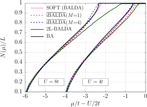
Figure 8: Lattice filling as a function of the chemical potential determined according to Eq. (31) for different approximations within P-SOET, and for the BALDA within SOFT. The curves correspond to $U=8t$ on the left side and $U=4t$ on the right side.

As readily seen in Fig. 8, $\overline{\rm iBALDA}$ does predict the opening of the charge gap with high accuracy, for both $U=4t$ and $U=8t$. Most impressively, only a single impurity site is sufficient to describe both the tendency of the exact curve as well as the actual position of the Mott transition. Increasing the number of impurities does not lead to any particular change. The transition seems to be also well reproduced within 2L-BALDA for $U=4t$, but the vanishing compressibility is manifested at $N(\mu)=398$ instead of the half-filled value $N(\mu)=400$. The same error arises for $U=8t$. Besides, the position of the Mott transition is not anymore correct and the value of the chemical potential is significantly overestimated compared to the BA results.

This striking result is a first for this type of embedding methods. It can be attributed to the additional use of accurate density functionals (BALDA here). Indeed, we can see that the BALDA curve within SOFT is almost on top of the BA results. The fact that BALDA is able to describe the opening of the charge gap (driven by non-local correlation effects in 1D Capone et al. (2004)) is due to the presence of a derivative discontinuity in the functional. This so-called “ultranonlocality” of BALDA (as opposed to the LDA in the continuum) has been extensively discussed by Ying et al. in Ref. Ying et al. (2014). To further stress on the importance of having a derivative discontinuity, we have proved in Appendix D of Ref. Senjean et al. (2018a) that the impurity correlation functional $E_{\rm c}^{\rm imp}(\mathbf{n})$ and the per-site correlation functional $e_{\rm c}(n)$ should manifest a derivative discontinuity at half-filling, while the bath correlation functional $\overline{E}_{\rm c}^{\rm bath}(\mathbf{n})$ should not. Even though the proof was derived in the atomic limit, we still think that the derivative discontinuity can be important for finite interaction strength. This condition is fulfilled by $\overline{\rm iBALDA}$ but not by 2L-BALDA (see the impurity correlation potential in Fig. 9 of Ref. Senjean et al. (2018b)), thus justifying why the Mott transition is better described within $\overline{\rm iBALDA}$. In DMFT, non-local effects can be described by considering a cluster rather than a single site Capone et al. (2004). A new formulation of SOET using the Green’s function formalism could provide a link between density functional contributions and the self-energy of the cluster, thus making a clearer connection between SOET and (cluster) DMFT. This is left for future work.

V Conclusions and perspectives

In this work, a new method so-called P-SOET has been derived from SOET by using the Schmidt decomposition. P-SOET is shown to give similar results as SOET but at a drastically reduced computational cost, thus allowing for calculations much closer to the thermodynamic limit. The use of the Schmidt decomposition makes P-SOET competitive with DMET Knizia and Chan (2012) and DET Bulik et al. (2014), with additional density functional contributions. As such, the embedding potential in P-SOET is analytical and is expressed as an energy derivative functional of the density, instead of being numerically optimized like in DMET. Accurate per-site energies and double occupations in the entire correlation regime and density domain have been obtained on the one-dimensional Hubbard model with 400 sites. As an important result, the density-driven Mott–Hubbard transition has been accurately predicted with a single impurity site. As far as we know, this is a first for this kind of embedding methods.

Note that SOET or P-SOET are not limited to the uniform one-dimensional Hubbard model and several extensions can be considered. First of all, (P-)SOET is straightforwardly applicable to higher-dimensional systems as the theory remains the same. The only requirement is that new appropriate functionals are needed. A recent work by Vilela et al. Vilela et al. (2019) could be used to derive a functional for the two- and three-dimensional Hubbard models from dimensional scaling of the BALDA functional. The description of heterogeneous systems can also be done by dividing the full system into multiple fragments. A global chemical potential would then be numerically optimized to ensure that the occupations of the fragments sum up to the total number of electrons, in the line of DMET. Magnetic and spin-dependent phenomena can also be addressed by including dependence on spin Franca et al. (2012) and on the current density Akande and Sanvito (2012) in the functional. The treatment of finite temperature effects would require a state-average theory and a temperature-dependent functional. While such functional could be relatively easily developed (see for instance Ref. Xianlong et al. (2012)), and the state-average extension comes naturally within SOET, P-SOET relies on the Schmidt decomposition which is state-dependent. The same problem arises in DMET. Note that an extension to excited states within DMET has been recently addressed by Tran et al. Tran et al. (2019). Their work could be used for similar developments in P-SOET. Turning to transport properties and the description of systems out of equilibrium, a real-time extension of P-SOET can be derived in analogy with real-time DMET Kretchmer and Chan (2018), together with time-dependent functionals that could be derived from earlier works on time-dependent lattice DFT Verdozzi (2008); Kurth et al. (2010); Karlsson et al. (2011); Kurth and Stefanucci (2017); Carrascal et al. (2018); Kurth and Stefanucci (2018). Alternatively, a frequency-dependent formulation of SOET could be derived using the Green’s function formalism. Finally, the extension to realistic systems like molecules (as done in DMFT Zgid and Chan (2011), DMET Knizia and Chan (2013); Wouters et al. (2016), and SEET Lan et al. (2015)) is maybe the most important one. Indeed, embedding approaches are appropriate to treat large systems in quantum chemistry due to their good balance between accuracy and computational cost (see Refs. Wesolowski et al. (2015); Lee et al. (2019b) and references therein). By decomposing the full system into subsystems, they are also promising candidates for solving classically intractable chemistry problems on near-term quantum devices Bauer et al. (2016); Rubin (2016); Reiher et al. (2017); Yamazaki et al. (2018) (see Ref. McArdle et al. (2018) for a review on quantum computational chemistry). By combining WFT and DFT, P-SOET would then be an efficient and free from double counting low cost embedding method able to treat both dynamical and static correlation effects of large chemical systems. Unfortunately, this extension is not straightforward as it faces fundamental issues like the dependence of the functionals on the molecular orbital basis Senjean (2018). Nevertheless, recent works on extending lattice DFT to quantum chemistry using localized orbitals Coe (2019) or also the domain separation in DFT Mosquera et al. (2019) could be helpful to generalize (P-)SOET to quantum chemistry. To get rid of the dependence on the molecular orbital basis, one could also work with the one-particle reduced density matrix as a variable instead of the occupation number only. P-SOET sheds a new light on the treatment of strongly correlated systems, and could progress in any of these aforementioned directions, which are under investigation. The ideas highlighted in this paper could hopefully inspire other works in the field.

VI Acknowledgments

BS is grateful to Emmanuel Fromager and Matthieu Saubanère for several fruitful discussions and meaningful comments on the article. BS thanks Matthieu Saubanère for providing him the Bethe Ansatz program. The DMRG calculations have been performed on the High-Performance Computing Center of the University of Strasbourg.

Appendix A Analytical solution for the Anderson dimer

The ground-state of the Anderson dimer is obtained by solving

$$\hat{H}^{\rm imp}|\Psi^{\rm imp}\rangle=\mathcal{E}^{\rm imp}|\Psi^{\rm imp}\rangle,$$ (32)

where

$$\hat{H}^{\rm imp}=-t\sum_{\sigma}\left(\hat{c}_{0\sigma}^{\dagger}\hat{c}_{1\sigma}+{\rm H.c.}\right)+U\hat{n}_{0\uparrow}\hat{n}_{0\downarrow}+\dfrac{\Delta v}{2}(\hat{n}_{1}-\hat{n}_{0})$$

and $\Delta v=v_{1}-v_{0}$. For two electrons, $\mathcal{E}^{\rm imp}$ has been shown to be related to the fully-interacting two-electron Hubbard dimer by a simple scaling and shifting relation Senjean et al. (2017):

$$\mathcal{E}^{\rm imp}(U,t,\Delta v)=E(U/2,t,\Delta v-U/2).$$ (34)

$E(U,t,\Delta v)$ is the ground-state singlet energy, solution of

$$-4t^{2}U+\left(4t^{2}-U^{2}+\Delta v^{2}\right)E+2UE^{2}=E^{3},$$ (35)

and can be expressed analytically as follows Carrascal et al. (2015):

$$E(u,t,\Delta v)=\dfrac{4t}{3}(u-w\sin(\dfrac{\pi}{6}+\theta)),$$ (36)

where

$$u = U/(2t),$$

$$w = \sqrt{3(1+\nu^{2})+u^{2}},$$

$$\nu = \Delta v/(2t),$$

$$\cos(3\theta) = (9(\nu^{2}-1/2)-u^{2})u/w^{3}.$$

According to the Hellmann–Feynman theorem, it follows from Eqs. (32) and (A) that the impurity occupation reads

$$n_{0} = 1-\dfrac{\partial\mathcal{E}^{\rm imp}(U,t,\Delta v)}{\partial\Delta v},$$ (37)

$$= 1-\left.\dfrac{\partial E(U,t,\Delta v)}{\partial\Delta v}\right|_{U=\overline{U},\Delta v=\overline{\Delta v}}.$$

where $\overline{U}=U/2$ and $\overline{\Delta v}=\Delta v-U/2$ are coming from the scaling and shifting relation in Eq. (34). Similarly, the off-diagonal element of the 1RDM of the Anderson dimer is given by

$$\gamma_{01} = -\dfrac{1}{2}\dfrac{\partial\mathcal{E}^{\rm imp}(U,t,\Delta v)}{\partial t}$$ (38)

$$= -\dfrac{1}{2}\left.\dfrac{\partial E(U,t,\Delta v)}{\partial t}\right|_{U=\overline{U},\Delta v=\overline{\Delta v}}$$

as well as the impurity double occupation,

$$d^{\rm imp} = \dfrac{\partial\mathcal{E}^{\rm imp}(U,t,\Delta v)}{\partial U}$$

$$= \dfrac{\partial U/2}{\partial U}\left.\dfrac{\partial E(U,t,\Delta v)}{\partial U}\right|_{U=\overline{U},\Delta v=\overline{\Delta v}}$$

$$+\dfrac{\partial\overline{\Delta v}}{\partial U}\left.\dfrac{\partial E(U,t,\Delta v)}{\partial\Delta v}\right|_{U=\overline{U},\Delta v=\overline{\Delta v}},$$

$$= \dfrac{1}{2}\left(\left.\dfrac{\partial E(U,t,\Delta v)}{\partial U}\right|_{U=\overline{U},\Delta v=\overline{\Delta v}}-(1-n_{0})\right).$$

The derivatives of the ground-state energy of the two-electron Hubbard dimer can be found by differentiating Eq. (35), thus leading to

$$\dfrac{\partial E}{\partial\Delta v} = \dfrac{2\Delta vE}{3E^{2}-4UE+U^{2}-4t^{2}-\Delta v^{2}},$$

$$\dfrac{\partial E}{\partial t} = \dfrac{8t(E-U)}{3E^{2}-4UE+U^{2}-4t^{2}-\Delta v^{2}},$$ (40)

$$\dfrac{\partial E}{\partial U} = \dfrac{2E(E-U)-4t^{2}}{3E^{2}-4UE+U^{2}-4t^{2}-\Delta v^{2}},$$

where $E$ is given by Eq. (36).

In P-SOET with a single impurity site, the embedded Hamiltonian reduces to the Hamiltonian of an Anderson dimer with two electrons that reads:

$$\hat{H}^{\rm emb}=\sum_{ij=0,\sigma}^{1}h^{\rm emb}_{ij}\left(\hat{c}_{i\sigma}^{\dagger}\hat{c}_{j\sigma}+{\rm H.c.}\right)+U\hat{n}_{0\uparrow}\hat{n}_{0\downarrow}.$$

The impurity occupation, the off-diagonal of the 1RDM and the impurity double occupation are calculating from Eqs. (37), (38) and (A) by replacing $t$ and $\Delta v$ by and $t=-h^{\rm emb}_{01}=-h^{\rm emb}_{10}>0$ and $\Delta v=h^{\rm emb}_{11}-h^{\rm emb}_{00}$.

Appendix B Self-consistency in P-SOET

B.1 Self-consistent procedure

SOET is a variational theory with respect to the density Fromager (2015); Senjean et al. (2017, 2018a, 2018b). This is different in P-SOET, which is split in two different part: the KS problem [Eq. (II.2.2)] and the embedded problem [Eq. (II.2.2)] obtained by projection of the effective Hamiltonian [Eq. (II.2.2)]. The solution of the KS problem is already obtained variationally and leads to the (in principle) exact density. The latter can be used to compute the embedding potential in the effective Hamiltonian and the expressions of the per-site energy and the double occupation [Eqs. (11) and (12), respectively]. This is the strategy employed in the main text.

In practice, approximate functionals lead to an approximate embedding potential that does not guarantee the recovering of the exact impurity occupations. This can be taken into account by updating the embedding potential self-consistently with the impurity occupations of the embedded problem [Eq. (26)]. Note that, for a uniform model, the knowledge of a single site occupation is in principle sufficient to determine the embedding potential exactly, providing that the exact bath Hxc functional (which itself depends on all sites occupation Senjean et al. (2017)) is known. One possible and practical way to reinsert the impurity occupations into the one-body effective Hamiltonian is to write:

$$\hat{h}^{\rm eff}=\hat{T}+\sum_{i=0}^{L-1}\left[\left.\dfrac{\partial\overline{E}^{\rm bath}_{{\rm Hxc},M}\left(\mathbf{n}\right)}{\partial n_{i}}\right|_{\mathbf{n}=\left\{\mathbf{n}^{\Psi^{\rm emb}_{M}},\mathbf{n}^{\rm bath}_{M}\right\}}\right]\hat{n}_{i},$$

where

$$\mathbf{n}^{\Psi^{\rm emb}_{M}}=\left\{n_{0}^{\Psi_{M}^{\rm emb}},n_{1}^{\Psi_{M}^{\rm emb}},\ldots,n_{M-1}^{\Psi_{M}^{\rm emb}}\right\}$$ (43)

is the impurity density (vector of size $M$) and

$$\mathbf{n}^{\rm bath}_{M}=\left\{\dfrac{1}{M}\sum_{i=0}^{M-1}n_{i}^{\Psi_{M}^{\rm emb}}\right\}$$ (44)

is the (uniform) bath density (vector of size $L-M$), determined by the mean-average of the impurity occupations. Note that other artificial choices (not considered here) could be made, like keeping the bath occupations frozen and equal to the ones obtained from the KS-SOFT calculation. The embedding potential obtained from the new density defines a new embedded problem, which we solve to obtain a new impurity density. This procedure is iterated until convergence of the impurity density is reached, as described in Fig. 9. This self-consistent loop can easily be added to Fig. 1 for completeness.

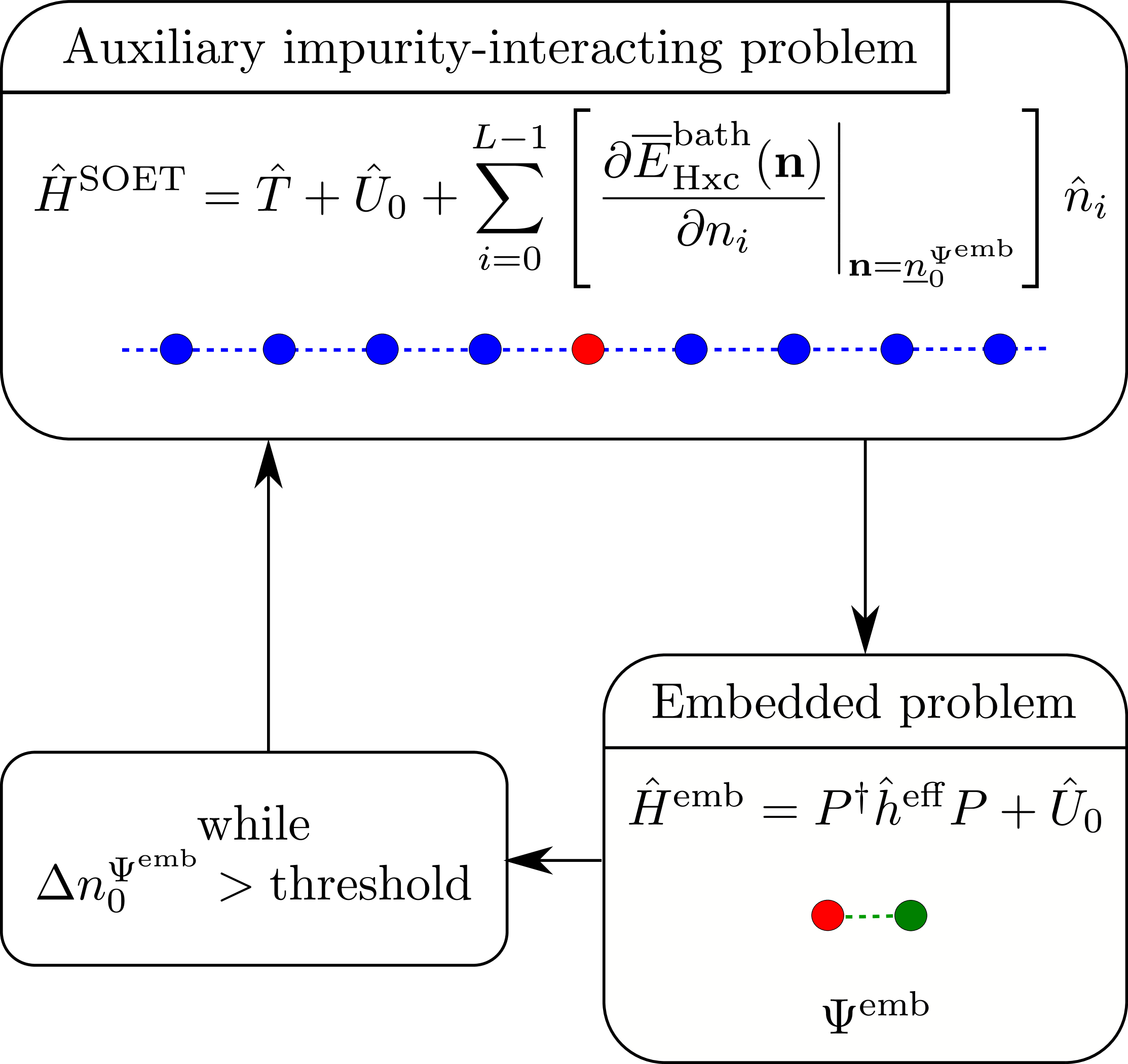
Figure 9: Self-consistent loop in P-SOET for a single impurity site. The projector is given by the Schmidt decomposition of the KS wavefunction (see Fig. 1).

One drawback of this self-consistent procedure is that the sum of the occupations in $\mathbf{n}^{\Psi^{\rm emb}_{M}}$ and $\mathbf{n}^{\rm bath}_{M}$ are not constrained to sum up to the total number of electrons. This could be fixed by optimizing the embedding potential of the embedded problem to reproduce the exact uniform density (obtained by solving the KS problem), in the line of DMET or DET for the correlation potential. For non-uniform models, one should divide the full system into multiple fragments, and the density of the full system would be rebuilt exactly by combining all the fragment occupations.

B.2 Self-consistent impurity occupations

The impurity occupations, determined self-consistently as described in the previous section, are shown in Fig. 10 for $U=4t$ (top panel) and $U=8t$ (bottom panel). Due to the boundary conditions, the impurity occupations in $\overline{\rm iBALDA}$($M$=4) are two-by-two equivalent, e.g. the impurities at the extremities of the fragment ($n_{0}=n_{3}$) and the ones in the middle of the fragment surrounded by the two other impurities ($n_{1}=n_{2}$). Therefore, only $n_{0}$ and $n_{1}$ are represented. As readily seen in Fig. 10, the deviation from the exact density is significant in the vicinity of half-filling. This would lead to strong density-driven errors in P-SOET in this regime. Note however that the 2L-BALDA occupation for $U=4t$ is accurate in the entire density domain. The deviations then increase for $U=8t$, showing that it is harder to converge to the correct density as the correlation strength increases.

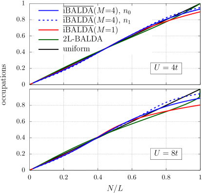
Figure 10: Impurity occupation(s) obtained self-consistently in P-SOET for different approximations, as a function of the exact uniform occupation $n=N/L$. We consider a system of $L=400$ sites with $U=4t$ (top panel) and $U=8t$ (bottom panel).

Interestingly, the occupations in Fig. 10 are really similar to the ones obtained from SOET (Figs. 7 and 8 of Ref. Senjean et al. (2018b)). This demonstrates the stability of this self-consistent procedure, which was not obvious considering the results of Table 1 showing that the impurity occupation obtained in P-SOET was not guaranteed to be the same as in SOET. Therefore, it seems that the self-consistent P-SOET is stable and gives similar results than SOET. To check this stability further, we start with other initial densities than the one obtained from the KS-SOFT calculation to determine the embedding potential in the effective problem [Eq. (II.2.2)]. Fig. 11 shows the impurity occupation within $\overline{\rm iBALDA}$($M$=1) at each iteration of the self-consistent procedure, starting from different initial densities. It is clear that the impurity occupation converges to the same value irrespective of the initial settings. Also, only a few number of iterations are needed, just like in self-consistent DMET but without the expensive fitting of the correlation potential at each iteration (for which alternatives have been recently developed Wu et al. (2019)). The difference between the converged occupation and the exact uniform one in Fig. 11 is mainly due to the use of approximate functionals, which determine the embedding potential [Eq. (8)].

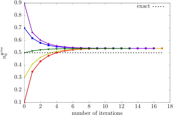
Figure 11: Impurity occupation within $\overline{\rm iBALDA}$($M$=1) at each iteration of the self-consistent procedure, starting from different uniform densities. The $L=400$ sites model is considered, with $N=200$ electrons and $U=10t$.

It is worth mentioning that convergence issues arise for $U\leqslant 1.8t$ at half-filling. Indeed, when the occupation is too close to 1, fluctuations of the occupations around 1 are known to appear due to the discontinuity in the potential Lima et al. (2003); Senjean et al. (2018b), as discussed in Sec. II.3. For $U\geqslant 1.8t$ the impurity occupations converge sufficiently far away from 1 to avoid this issue. Appart from that, we have not observed any convergence problem in this self-consistent formulation of P-SOET.

References

- Hohenberg and Kohn (1964) P. Hohenberg and W. Kohn, Phys. Rev. 136, B864 (1964).
- Kohn and Sham (1965) W. Kohn and L. Sham, Phys. Rev. 140, A1133 (1965).
- Cohen et al. (2011) A. J. Cohen, P. Mori-Sánchez, and W. Yang, Chem. Rev. 112, 289 (2011).
- Swart (2013) M. Swart, Int. J. Quantum Chem. 113, 2 (2013).
- Swart and Gruden (2016) M. Swart and M. Gruden, Acc. Chem. Res. 49, 2690 (2016).
- Sun and Chan (2016) Q. Sun and G. K.-L. Chan, Acc. Chem. Res. 49, 2705 (2016).
- Georges and Kotliar (1992) A. Georges and G. Kotliar, Phys. Rev. B 45, 6479 (1992).
- Georges et al. (1996) A. Georges, G. Kotliar, W. Krauth, and M. J. Rozenberg, Rev. Mod. Phys. 68, 13 (1996).
- Kotliar and Vollhardt (2004) G. Kotliar and D. Vollhardt, Phys. Today 57, 53 (2004).
- Kotliar et al. (2006) G. Kotliar, S. Y. Savrasov, K. Haule, V. S. Oudovenko, O. Parcollet, and C. A. Marianetti, Rev. Mod. Phys. 78, 865 (2006).
- Held (2007) K. Held, Adv. Phys. 56, 829 (2007).
- Vollhardt et al. (2012) D. Vollhardt, K. Byczuk, and M. Kollar, in Strongly Correlated Systems (Springer, 2012) pp. 203–236.
- Martin et al. (2016) R. M. Martin, L. Reining, and D. M. Ceperley, Interacting Electrons (Cambridge University Press, 2016).
- Kananenka et al. (2015) A. A. Kananenka, E. Gull, and D. Zgid, Phys. Rev. B 91, 121111 (2015).
- Lan et al. (2015) T. N. Lan, A. A. Kananenka, and D. Zgid, J. Chem. Phys. 143, 241102 (2015).
- Lan et al. (2016) T. N. Lan, A. A. Kananenka, and D. Zgid, J. Chem. Theory Comput. 12, 4856 (2016).
- Zgid and Gull (2017) D. Zgid and E. Gull, New J. Phys. 19, 023047 (2017).
- Lan et al. (2017) T. N. Lan, A. Shee, J. Li, E. Gull, and D. Zgid, Phys. Rev. B 96, 155106 (2017).
- Tran et al. (2018) L. N. Tran, S. Iskakov, and D. Zgid, J. Phys. Chem. Lett. 9, 4444 (2018).
- Rusakov et al. (2018) A. A. Rusakov, S. Iskakov, L. N. Tran, and D. Zgid, J. Chem. Theory Comput. 15, 229 (2018).
- Knizia and Chan (2012) G. Knizia and G. K.-L. Chan, Phys. Rev. Lett. 109, 186404 (2012).
- Bulik et al. (2014) I. W. Bulik, G. E. Scuseria, and J. Dukelsky, Phys. Rev. B 89, 035140 (2014).
- Welborn et al. (2016) M. Welborn, T. Tsuchimochi, and T. Van Voorhis, J. Chem. Phys. 145, 074102 (2016).
- Ricke et al. (2017) N. Ricke, M. Welborn, H.-Z. Ye, and T. Van Voorhis, Mol. Phys. 115, 2242 (2017).
- Ye et al. (2018) H.-Z. Ye, M. Welborn, N. D. Ricke, and T. Van Voorhis, J. Chem. Phys. 149, 194108 (2018).
- Mordovina et al. (2019) U. Mordovina, T. E. Reinhard, H. Appel, and A. Rubio, arXiv:1901.07658 (2019).
- Knizia and Chan (2013) G. Knizia and G. K.-L. Chan, J. Chem. Theory Comput. 9, 1428 (2013).
- Wouters et al. (2016) S. Wouters, C. A. Jiménez-Hoyos, Q. Sun, and G. K.-L. Chan, J. Chem. Theory Comput. 12, 2706 (2016).
- Zheng et al. (2017a) B.-X. Zheng, J. S. Kretchmer, H. Shi, S. Zhang, and G. K.-L. Chan, Phys. Rev. B 95, 045103 (2017a).
- Pham et al. (2018) H. Q. Pham, V. Bernales, and L. Gagliardi, J. Chem. Theory Comput. 14, 1960 (2018).
- Hermes and Gagliardi (2019) M. R. Hermes and L. Gagliardi, J. Chem. Theory Comput. 15, 972 (2019).
- LeBlanc et al. (2015) J. P. F. LeBlanc, A. E. Antipov, F. Becca, I. W. Bulik, G. K.-L. Chan, C.-M. Chung, Y. Deng, M. Ferrero, T. M. Henderson, C. A. Jiménez-Hoyos, E. Kozik, X.-W. Liu, A. J. Millis, N. V. Prokof’ev, M. Qin, G. E. Scuseria, H. Shi, B. V. Svistunov, L. F. Tocchio, I. S. Tupitsyn, S. R. White, S. Zhang, B.-X. Zheng, Z. Zhu, and E. Gull, Phys. Rev. X 5, 041041 (2015).
- Zheng and Chan (2016) B.-X. Zheng and G. K.-L. Chan, Phys. Rev. B 93, 035126 (2016).
- Tsuchimochi et al. (2015) T. Tsuchimochi, M. Welborn, and T. Van Voorhis, J. Chem. Phys. 143, 024107 (2015).
- Fan and Jie (2015) Z. Fan and Q.-l. Jie, Phys. Rev. B 91, 195118 (2015).
- Gunst et al. (2017) K. Gunst, S. Wouters, S. De Baerdemacker, and D. Van Neck, Phys. Rev. B 95, 195127 (2017).
- Zheng et al. (2017b) B.-X. Zheng, C.-M. Chung, P. Corboz, G. Ehlers, M.-P. Qin, R. M. Noack, H. Shi, S. R. White, S. Zhang, and G. K.-L. Chan, Science 358, 1155 (2017b).
- Sandhoefer and Chan (2016) B. Sandhoefer and G. K.-L. Chan, Phys. Rev. B 94, 085115 (2016).
- Reinhard et al. (2019) T. E. Reinhard, U. Mordovina, C. Hubig, J. S. Kretchmer, U. Schollwöck, H. Appel, M. A. Sentef, and A. Rubio, J. Chem. Theory Comput. 15, 2221 (2019).
- Mukherjee and Reichman (2017) S. Mukherjee and D. R. Reichman, Phys. Rev. B 95, 155111 (2017).
- Chen et al. (2014) Q. Chen, G. H. Booth, S. Sharma, G. Knizia, and G. K.-L. Chan, Phys. Rev. B 89, 165134 (2014).
- Booth and Chan (2015) G. H. Booth and G. K.-L. Chan, Phys. Rev. B 91, 155107 (2015).
- Kretchmer and Chan (2018) J. S. Kretchmer and G. K.-L. Chan, J. Chem. Phys. 148, 054108 (2018).
- Fertitta and Booth (2018) E. Fertitta and G. H. Booth, Phys. Rev. B 98, 235132 (2018).
- Lee et al. (2019a) T.-H. Lee, T. Ayral, Y.-X. Yao, N. Lanata, and G. Kotliar, Phys. Rev. B 99, 115129 (2019a).
- Fromager (2015) E. Fromager, Mol. Phys. 113, 419 (2015).
- Senjean et al. (2017) B. Senjean, M. Tsuchiizu, V. Robert, and E. Fromager, Mol. Phys. 115, 48 (2017).
- Senjean et al. (2018a) B. Senjean, N. Nakatani, M. Tsuchiizu, and E. Fromager, Phys. Rev. B 97, 235105 (2018a).
- Senjean et al. (2018b) B. Senjean, N. Nakatani, M. Tsuchiizu, and E. Fromager, Theor. Chem. Acc. 137, 169 (2018b).
- Senjean (2018) B. Senjean, Development of new embedding techniques for strongly correlated electrons : from in-principle-exact formulations to practical approximations., Ph.D. thesis, Université de Strasbourg (2018).
- Gunnarsson and Schönhammer (1986) O. Gunnarsson and K. Schönhammer, Phys. Rev. Lett. 56, 1968 (1986).
- Schönhammer et al. (1995) K. Schönhammer, O. Gunnarsson, and R. Noack, Phys. Rev. B 52, 2504 (1995).
- Note (1) We have tried to use a different projector generated from the ground-state of the effective Hamiltonian [Eq. (II.2.2)] instead of the KS Hamiltonian [Eq. (II.2.2)], but it led to insufficiently accurate results.
- Ayral et al. (2017) T. Ayral, T.-H. Lee, and G. Kotliar, Phys. Rev. B 96, 235139 (2017).
- Wu et al. (2019) X. Wu, Z.-H. Cui, Y. Tong, M. Lindsey, G. K.-L. Chan, and L. Lin, arXiv:1905.00886 (2019).
- Lima et al. (2002) N. Lima, L. Oliveira, and K. Capelle, Europhys. Lett. 60, 601 (2002).
- Lima et al. (2003) N. A. Lima, M. F. Silva, L. N. Oliveira, and K. Capelle, Phys. Rev. Lett. 90, 146402 (2003).
- Capelle et al. (2003) K. Capelle, N. Lima, M. Silva, and L. Oliveira, in The Fundamentals of Electron Density, Density Matrix and Density Functional Theory in Atoms, Molecules and the Solid State (Springer, 2003) p. 145.
- Chan and Head-Gordon (2002) G. K.-L. Chan and M. Head-Gordon, J. Chem. Phys. 116, 4462 (2002).
- Chan (2004) G. K.-L. Chan, J. Chem. Phys. 120, 3172 (2004).
- Ghosh et al. (2008) D. Ghosh, J. Hachmann, T. Yanai, and G. K.-L. Chan, J. Chem. Phys. 128, 144117 (2008).
- Sharma and Chan (2012) S. Sharma and G. K.-L. Chan, J. Chem. Phys. 136, 124121 (2012).
- Olivares-Amaya et al. (2015) R. Olivares-Amaya, W. Hu, N. Nakatani, S. Sharma, J. Yang, and G. K.-L. Chan, J. Chem. Phys. 142, 034102 (2015).
- (64) B. Senjean, [Online]. https://github.com/bsenjean/P-SOET.
- Lieb and Wu (1968) E. H. Lieb and F. Y. Wu, Phys. Rev. Lett. 20, 1445 (1968).
- Shiba (1972) H. Shiba, Phys. Rev. B 6, 930 (1972).
- Lieb and Wu (2003) E. H. Lieb and F. Y. Wu, Physica A 321, 1 (2003).
- Capone et al. (2004) M. Capone, M. Civelli, S. Kancharla, C. Castellani, and G. Kotliar, Phys. Rev. B 69, 195105 (2004).
- Ying et al. (2014) Z.-J. Ying, V. Brosco, and J. Lorenzana, Phys. Rev. B 89, 205130 (2014).
- Vilela et al. (2019) L. N. Vilela, K. Capelle, L. N. Oliveira, and V. L. Campo, arXiv:1904.10529 (2019).
- Franca et al. (2012) V. V. Franca, D. Vieira, and K. Capelle, New J. Phys. 14, 073021 (2012).
- Akande and Sanvito (2012) A. Akande and S. Sanvito, J. Phys. Condens. Matter 24, 055602 (2012).
- Xianlong et al. (2012) G. Xianlong, A.-H. Chen, I. Tokatly, and S. Kurth, Phys. Rev. B 86, 235139 (2012).
- Tran et al. (2019) H. K. Tran, T. Van Voorhis, and A. J. Thom, J. Chem. Phys. 151, 034112 (2019).
- Verdozzi (2008) C. Verdozzi, Phys. Rev. Lett. 101, 166401 (2008).
- Kurth et al. (2010) S. Kurth, G. Stefanucci, E. Khosravi, C. Verdozzi, and E. K. U. Gross, Phys. Rev. Lett. 104, 236801 (2010).
- Karlsson et al. (2011) D. Karlsson, A. Privitera, and C. Verdozzi, Phys. Rev. Lett. 106, 116401 (2011).
- Kurth and Stefanucci (2017) S. Kurth and G. Stefanucci, J. Phys. Condens. Matter 29, 413002 (2017).
- Carrascal et al. (2018) D. J. Carrascal, J. Ferrer, N. Maitra, and K. Burke, Eur. Phys. J. B 91, 142 (2018).
- Kurth and Stefanucci (2018) S. Kurth and G. Stefanucci, Eur. Phys. J. B 91, 118 (2018).
- Zgid and Chan (2011) D. Zgid and G. K.-L. Chan, J. Chem. Phys. 134 (2011), 10.1063/1.3556707.
- Wesolowski et al. (2015) T. A. Wesolowski, S. Shedge, and X. Zhou, Chem. Rev. 115, 5891 (2015).
- Lee et al. (2019b) S. J. Lee, M. Welborn, F. R. Manby, and T. F. Miller III, Acc. Chem. Res. 52, 1359 (2019b).
- Bauer et al. (2016) B. Bauer, D. Wecker, A. J. Millis, M. B. Hastings, and M. Troyer, Phys. Rev. X 6, 031045 (2016).
- Rubin (2016) N. C. Rubin, arXiv:1610.06910 (2016).
- Reiher et al. (2017) M. Reiher, N. Wiebe, K. M. Svore, D. Wecker, and M. Troyer, Proc. Natl. Acad. Sci. U.S.A. 114, 7555 (2017).
- Yamazaki et al. (2018) T. Yamazaki, S. Matsuura, A. Narimani, A. Saidmuradov, and A. Zaribafiyan, arXiv:1806.01305 (2018).
- McArdle et al. (2018) S. McArdle, S. Endo, A. Aspuru-Guzik, S. Benjamin, and X. Yuan, arXiv:1808.10402 (2018).
- Coe (2019) J. P. Coe, Phys. Rev. B 99, 165118 (2019).
- Mosquera et al. (2019) M. A. Mosquera, L. O. Jones, C. H. Borca, M. A. Ratner, and G. C. Schatz, J. Phys. Chem. A 123, 4785 (2019).
- Carrascal et al. (2015) D. J. Carrascal, J. Ferrer, J. C. Smith, and K. Burke, J. Phys. Condens. Matter 27, 393001 (2015).