Wormhole as a possible accelerator of high-energy cosmic-ray particles

Abstract

We present the simplest topological classification of wormholes and demonstrate that in open Friedmann models the genus $n\geq 1$ wormholes are stable and do not require the presence of exotic forms of matter, or any modification of general relativity. We show that such wormholes may also possess magnetic fields. It is found that when the wormhole gets into a galaxy or a surrounding region, it works as an accelerator of charged particles. If the income of the energy from radiation is small, such a wormhole works simply as a generator of synchrotron radiation. Estimates show that the threshold energy of such an accelerator may vary from sufficiently modest energies of the order of a few Gev, up to enormous energies of the Planckian order and even higher, depending on wormhole parameters.

I Introduction

One of the great challenges of modern astrophysics is the origin of the observed high-energy cosmic-ray particles (HECRs) Pierre Auger Collaboration (2010); DAMPE Collaboration (2017). There are a number of high-energy processes in galaxies which may serve as likely candidates of such extremely energetic particles, e.g., active galactic nuclei, jets in radio galaxies, etc. Hillas (1984); Eichmann et. al. (2018). HECRs may also be related to the decay of dark matter particles Feng (2010); Grib & Pavlov (2009); Belotsky, et al. (2014, 2015). Still the nature of their origin is not firmly established. In the present paper we suggest a new possible mechanism which may allow to accelerate charged particles till extremely high energies. Such a mechanism involves wormholes whose existence is predicted by general relativity and essentially by different extensions of gravity e.g., see Visser (1996); Hochberg et al. (1997); Harko et al. (2013); Myrzakulov et al. (2016); Lobo (2017).

It is expected that relic cosmological wormholes were created from virtual wormholes on quantum stage, or during the inflationary period of evolution of the Universe. In general relativity without exotic matter spherically symmetric wormholes are non-static objects e.g., see Arellano & Lobo (2006), and they presumably collapse very rapidly. However they may be static in various extended theories where the role of exotic matter is played by a modification of general relativity. It was recently shown that in the Einstein’s theory stable quasi-stationary wormholes without exotic matter do exist in open Friedmann models Kirillov & Savelova (2016). Such wormholes have a more general structure and have throat sections in the form of tori or more complicated surfaces. General consideration shows that in the flat space static wormholes of such a kind also require the presence of some portion of exotic matter. In the absence of exotic forms of matter such wormholes do evolve. Still it is not clear how rapid is the rate of their evolution.

Some encouraging results were obtained in the limit when one radius of a torus-like throat tends to infinity. Then the geometry acquires cylindrical configuration. In particular, in a series of papers Bronnikov et al. (2013); Bronnikov & Lemos (2009); Bronnikov & Krechet (2019a); Bronnikov et al. (2019b) static and stationary cylindrical wormhole solutions were found and it was demonstrated that asymptotically flat wormhole configurations do not require exotic matter violating the weak energy condition.

Primordial wormholes may initially capture some electric and magnetic lines of force. Therefore, from the formal standpoint every entrance into wormhole throat will look as if it were carrying some electric and magnetic charges, e.g., see exact solutions in Arellano & Lobo (2006). Of course the two entrances into the same wormhole have charges of opposite signs as it should be. In other words, it is more correct here to speak of electric and magnetic poles of different entrances. Therefore, in the general case every entrance into such primordial wormholes can be described by a mass, an angular momentum, an electric charge, and a magnetic charge as well. During the evolution the electric charge decays very rapidly, since the electric field transmits straightforwardly its energy to charged particles in the primordial plasma. The magnetic part however do not perform the work and retains. Therefore, it is natural to expect that magnetic fields (magnetic lines captured by wormholes) survive and may play the role of the seeds which generate magnetic fields in intergalactic medium. For example, this may explain the origin of observed magnetic fields in voids Planck Collaboration (2016).

It turns out that in galaxies such a wormhole may work as an accelerator of charged particles or simply as a generator of the synchrotron radiation. Indeed, charged particles captured by magnetic field of a wormhole may move only along magnetic lines which start from one entrance and end on the another entrance. Therefore, they are captured by such a wormhole. The galactic wind produced by a galaxy and the active galactic nuclear push such particles and speeds them up. Part of the received energy reradiates as the synchrotron radiation. This acceleration continues till the moment when particles reach the stationary state (when the received and reradiated energies become equal), or till the moment when they gain enough energy to escape the magnetic trap. In general there exists some threshold for the energy of such particles (the maximal possible value) which is completely determined by wormhole parameters and the activity of the galaxy. Moreover, the same wind acts on the magnetic field of the wormhole and may rotate it to the equilibrium position, when the direction of magnetic lines coincides with the direction of the wind. This makes the accelerator to work more efficiently. We may expect that at least part of high-energy cosmic rays may be produced by such a scheme. This also may explain the recently reported break in the teraelectronvolt cosmic-ray spectrum of electrons and positrons DAMPE Collaboration (2017). Indeed the two branches of such a spectrum correspond simply to two different such wormhole accelerators, while the position of the brake corresponds to the threshold energy for the nearest wormhole.

II Topological structure of a general genus $n$ wormhole

According to the Geroch theorem Geroch (1967) in general relativity the topological structure of space does not change. Indeed, consider the Hamiltonian formulation of general relativity. The metric of the space-time has the form

$$ds^{2}=N^{2}dt-g_{\alpha\beta}\left(dx^{\alpha}+N^{\alpha}dt\right)\left(dx^{\beta}+N^{\beta}dt\right),$$ (1)

where  $N$ is the lapse function, $N^{\alpha}$ is the shift vector and $g_{\alpha\beta}$ is the metric of a space-like manifold $S$. In the Hamiltonian picture functions $N$ and $N^{\alpha}$ have no dynamic character and they play the role of Lagrange multipliers, while the Hamiltonian is

$$H=\int\limits_{S}\left(NC+N^{\alpha}C_{\alpha}\right)d^{3}x,$$ (2)

where

$$C=\frac{1}{\sqrt{g}}\left[\pi^{\alpha\beta}\pi_{\alpha\beta}-\frac{1}{2}\left(\pi_{\alpha}^{\alpha}\right)^{2}+g\left(-P\right)\right],$$ (3)

$$C_{\alpha}=-2\nabla_{\beta}\pi_{\alpha}^{\beta}.$$ (4)

Here $P$ is the curvature scalar with the 3-dimensional metric $g_{\alpha\beta}$, $\nabla_{\alpha}$ defines the covariant derivative with the metric $g_{\alpha\beta}$, and we assume that $S$ is closed space-like hypersurface (to avoid surface terms in the action). In the presence of matter fields one has to add respective terms to the Hamiltonian. The equations of motion have the standard form

$$\frac{dg_{\alpha\beta}}{dt}=\frac{\delta H}{\delta\pi^{\alpha\beta}},\ \ \frac{d\pi^{\alpha\beta}}{dt}=-\frac{\delta H}{\delta g_{\alpha\beta}},$$ (5)

while the variation of the action with respect to lapse and shift gives the constraints ($G_{\alpha}^{0}$ components of the Einstein equations)

$$C=0,\ \ C_{\alpha}=0.$$ (6)

Taken the initial values $\left(g_{\alpha\beta},\pi^{\alpha\beta}\right)$ on $S$ at some moment of time $t=t_{0}$, the above equations define in a unique way the subsequent evolution of the dynamic functions $\left(g_{\alpha\beta}(t),\pi^{\alpha\beta}(t)\right)$. This defines the map of the space-like hypersurfaces $S(t_{0})\rightarrow S(t)$ which is a diffeomorphism between $S(t_{0})$ and $S(t)$ (differentiable one-to-one map). Thus in the Hamiltonian picture we see that the topological structure of the total space-time always represents the direct product of the topology of the initial hypersurface $S(t_{0})$ and the time line $t\in R^{1}$. This is roughly constitute the famous Geroch theorem, which states that in general relativity topology changes do not occur. We point out that there exist some speculations based on the fact that choosing different space-like sections of a single maximally extended space-time we may obtain different topologies of space-like sections. Some authors try to interpret this as ”topology changes”. But the observer may try different reference frames and easily verify that such a change is nothing more, than the effect related to a specific frame. Therefore, such interpretations are not self-consistent from the physical standpoint.

In this manner we see that in general relativity topological structure of space is determined by onset, as additional initial conditions. In other words, it is specified by hands. In conclusion of this section we define topologies which correspond to a general genus $n$ wormhole (e.g., see the books Fomenko (1999); Hempel (1976); Visser (1996)).

Consider two copies $\partial M_{n}^{\pm}$ of an arbitrary two dimensional closed surface $\partial M_{n}$ in $S$. From the topological standpoint the surface $\partial M_{n}$ represents a sphere with $n$ handles on it. The portion of space $S$ which gets inside such surfaces $x\in M_{n}^{\pm}$ is removed, while points on respective two copies of the surfaces $\partial M_{n}^{\pm}$ are glued. This corresponds to the so-called Hegor diagrams Fomenko (1999); Hempel (1976). Thus, we get a wormhole whose throat section is $\partial M_{n}$ which is sphere with $n$ handles. The number of handles $n$ is called the genus of two dimensional surface and we keep this name for the wormhole. Thus we get a wormhole of the genus $n$. The resulting space is $S_{n}=S/M_{n}^{\pm}$ and it’s structure determines properties of possible initial conditions $\left(g_{\alpha\beta}(t_{0}),\pi^{\alpha\beta}(t_{0})\right)$ which can be specified on $S_{n}$. In particular, since points on surfaces $\partial M_{n}^{+}$ and $\partial M_{n}^{-}$ are identical, the admissible functions $\left(g_{\alpha\beta}(t_{0}),\pi^{\alpha\beta}(t_{0})\right)$ should obey the respective periodic conditions, namely, they should coincide on $\partial M_{n}^{+}$ and $\partial M_{n}^{-}$ and possess the necessary number of derivatives. The subsequent evolution is completely determined by the above Hamiltonian equations.

In the case when the distance between surfaces $\partial M_{n}^{+}$ and $\partial M_{n}^{-}$ is sufficiently big, the influence of the entrances into the wormhole on each other can be neglected. In this case we may restrict to a wormhole which connects two different copies of the space $S$. We may call them as two-wold wormholes, contrary to the previous case when both entrances lay in the same space. The two-wold wormholes are more simple for the investigation and gain more popularity in literature.

We point out that topology of space was formed (tempered) during quantum stage of the evolution of our Universe and a priory all kind of wormholes are admissible as initial conditions. However subsequent evolution is quite different. In particular, the simplest wormholes of the genus $n=0$ are highly unstable. To be stable they requite the presence of exotic matter which does not exist in nature. Genus $n=0$ wormholes may be made stable in modified theories in which exotic matter is replaced by an appropriate modification. In other words, in the standard Einstein’s general relativity such wormholes collapse and are undistinguished from black holes. This means that in spite the widespread popularity of such solutions (i.e., spherically symmetric wormholes) we should not expect to find such objects in astrophysics unless the appropriate modification is experimentally established.

III Stable relic wormholes

In general relativity stable relic wormhole cannot have the genus $n=0$. There is an extended literature on this subject and we may send readers to respective books and reviews, e.g., Visser (1996); Lobo (2017).

In this section we demonstrate that genus $n\geq 1$ wormholes can be made stable in open Friedmann models, as it was first shown in Kirillov & Savelova (2016). The basic idea comes out from very simple qualitative consideration as follows. Since the section of a wormhole throat $\partial M_{n}$ is closed, its size is always restricted in space. When we consider the scattering of a thin ray of particles on such a wormhole it always diverges upon scattering. This means that the wormhole throat has always a negative curvature. Therefore, to find the simplest realization of such a topology we should use the open cosmological model in which space has a constant negative curvature. We recall that observational bounds allow our Universe to have very small negative curvature (within the observational errors Planck Collaboration (2016, 2018) $\Omega_{k}=0.001\pm 0.002$). Moreover, even if our Universe is exactly flat, it contains both overdense regions which possess a positive curvature and underdense regions with a negative curvature. The latter in some approximation can be viewed as parts of the Lobachevsky space. Then, as it was first demonstrated in Kirillov & Savelova (2016) an arbitrary number of genus $n\geq 1$ wormholes can be constructed simply by factorization of the Lobachevsky space (the space of the open Friedmann model) over a discrete subgroup of the group of motion of the Lobachevsky space.

We point out that the genus $n=0$ wormhole cannot be obtained by such a factorization, since the sphere does not admit the metric with a negative curvature. When we try to specify a negative curvature on the sphere, it will contain at least one singular point. The simplest wormhole (whose existence do not require exotic matter) has the genus $n=1$ which corresponds to the throat section in the form of a torus. For details we send readers to our paper mentioned before.

For the illustration of the basic idea we describe the realization of the simplest two-dimensional wormhole which connects two different spaces by a factorization of the Lobachevsky plane. Consider the open Friedmann model which is described by the metric

$$ds^{2}=c^{2}dt^{2}-a^{2}(t)\frac{4(dx^{2}+dy^{2}+dz^{2})}{\left(1-r^{2}\right)^{2}}.$$ (7)

Here the space metric $dl^{2}=\frac{4dx^{2}}{\left(1-x^{2}\right)^{2}}$ corresponds to the Lobachevsky space. In 2D case the space can be realized as a upper complex half -plane Fig1, when the metric takes the form ($z=x+iy$, $y>0$)

$$dl^{2}=\frac{dx^{2}+dy^{2}}{y^{2}}.$$ (8)

In this metric the line $y=0$ corresponds to the absolute, i.e., the infinity of the Lobachevsky plane). Consider now two an arbitrary geodesic lines on the Lobachevsky plane. To avoid misunderstanding we stress that we are speaking here of space-like geodesics on the Lobachevsky plane (do not mix them with space-time geodesics that correspond to motions of probe particles). Recall that geodesics on the plane are semi-circles with centers on the absolute $y=0$ and perpendicular to the absolute rays ($y=const$). Using the group of motions of the plane we may choose the coordinate frame on the plane in such a way that the both geodesics become semi-circles with centers at the origin $z=0$ but having different radii $R_{1}$ and $R_{2}$. For definiteness we assume $R_{1}>R_{2}$. Then the geodesic line $y=0$ determines the shortest distance between these two geodesics. According to (8) we see that the distance is simply $a=\ln\left(R_{1}/R_{2}\right)$. The simplest wormhole is obtained by making the cut of the stripe between these two geodesics and the subsequent gluing of the boundaries (the two geodesics) see Fig 1. The regions on the plane which are restricted by auxiliary two geodesic lines with the radius $r=\left(R_{1}-R_{2}\right)/2$ and centers at the positions $x_{\pm}=\pm(R_{2}+r)$ correspond to two different Lobachevsky spaces (any geodesic there has infinite length). The rest part of the stripe has a finite square/volume and corresponds to the throat of the wormhole.

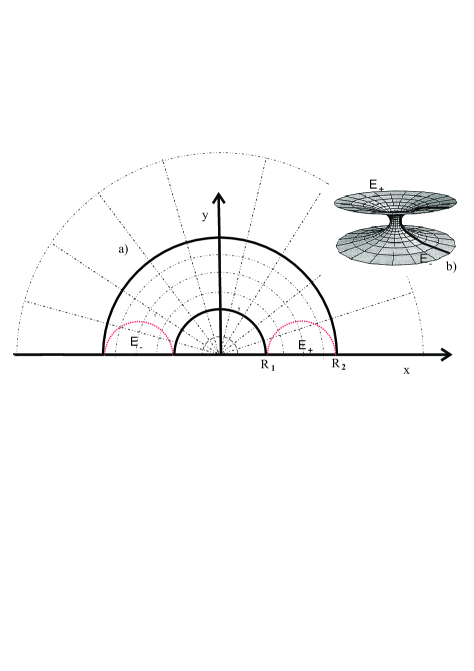
Figure 1: a)The Lobachevsky plane. Dashed lines give the polar frame. The stripe between the two geodesic lines $r=R_{1}$ and $r=R_{2}$ corresponds to the wormhole region. Regions below red dashed geodesics (semi-circles) correspond to two unrestricted Lobschevsky spaces $E_{\pm}$. b) The same wormhole which connects two Lobachevsky spaces $E_{\pm}$. Thick solid line corresponds to the two geodesics $r=R_{1,2}$ on the plane which are glued.

Consider the particular motion $T_{a}$ of the plane that transforms one geodesic (of the radius $R_{2}$) to the other ($R_{1}$). This is reached by the transformation

$$z^{\prime}=T_{a}(z)=\frac{R_{1}}{R_{2}}z=e^{a}z.$$ (9)

This transformation corresponds to the shift of the plane along the geodesic line $y=0$ on the distance $a$. One can straightforwardly verify that this transformation does not change the metric (8) and, therefore, it is one of particular admissible motions of the plane. Using $T_{a}$ as the basis element we define the discrete subgroup $G_{a}$ of the group of motions of the plane which consists of all elements of the form $\{T_{a}^{n}\}$, where $n=0,\pm 1,\pm 2,...$. Then the wormhole is merely the factorization of the plane over $G_{a}$. This means that any two points of the plane $z$ and $z^{\prime}$ correspond to the same single point of the wormhole, if they can be related by the transformation $z^{\prime}=\left(R_{1}/R_{2}\right)^{n}z=e^{na}z$ with any integer $n$.

The basic difference between the wormhole and the total Lobachevsky plane is that now we cannot specify an arbitrary functions on the plane. Those are restricted by a specific ”periodic” conditions. For example, if we consider perturbations of the metric $\delta g_{\alpha\beta}(z)$, then they should obey the ”periodic” property

$$\delta g_{\alpha\beta}(z)=\delta g_{\alpha\beta}(\frac{R_{1}}{R_{2}}z).$$ (10)

In particular, our attempts to describe dark matter phenomena by wormholes Kirillov & Savelova (2008, 2011) owe to this feature. Indeed, if we have a point source $M$ at some position $z_{0}$ (the density is $\varrho=\frac{M}{\sqrt{g}}\delta(z-z_{0})$), then the condition (10) produces a countable set of ”additional” sources ($\varrho\rightarrow\varrho=\frac{M}{\sqrt{g}}\sum_{n}\delta(z-e^{na}z_{0})$) and this essentially changes the ”expected” standard Newton’s potential produced by the source, while the transformation $\delta(z-z_{0})\rightarrow\sum_{n}\delta(z-e^{na}z_{0})$ we call the topological bias of sources. This additional images may play the role of dark matter particles.

We point out that in the case of 3D Lobachevsky space the simplest 3D wormhole is obtained by analogous factorization over the discrete subgroup that is formed from two such generators $T_{a}(l_{1})$ and $T_{b}(l_{2})$ which describe two such shifts in orthogonal directions ($l_{1}$ and $l_{2}$ denote two orthogonal geodesics). In this case the minimal section of the throat will have the form of a torus $T^{2}$.

Such a factorization can be straightforwardly seen in terms of new coordinate frame which can be introduced on the Lobachevsky space. Indeed, consider realization of 3D Lobachevsky space in the form of half space analogous to (8) which is given by the metric

$$dl^{2}=\frac{dx^{2}+dy^{2}+dz^{2}}{z^{2}}$$ (11)

where $z>0$. Consider first the transformation $T_{a}(l_{1})$. Using possible motions of the space any map $T_{a}(l_{1})$ can be realized as the conformal transformation $T_{a}\left(r,\phi,\theta\right)=\left(\frac{R_{1}}{R_{2}}r,\phi,\theta\right)$, where we have used the spherical coordinate frame $x=r\cos\phi\sin\theta$, $y=r\sin\phi\sin\theta$, $z=r\cos\theta$, with variables ranges as $r>0$, $0<\theta<\frac{\pi}{2}$, and $0<\phi<2\pi$. In this coordinates the 2D Lobachevsky plane Fig 1. corresponds to any section $\phi=const$. In this realization the geodesic line $l_{1}$ corresponds simply to the axis $z$ ($l_{1}=(0,0,z)$). Then we may use the subsequent transformation in the form $r=R_{2}$ $\exp\left(\frac{a}{2\pi}\chi_{1}\right)$ which transforms the line element into

$$dl^{2}=\frac{1}{\cos^{2}\theta}\left(\left(\frac{a}{2\pi}\right)^{2}d\chi_{1}^{2}+\sin^{2}\theta d\phi^{2}+d\theta^{2}\right).$$ (12)

The region $R_{2}<r<R_{1}$ corresponds to the range of the new angle variable $0<\chi_{1}<2\pi$, while the total space corresponds to the unrestricted range of the variable $\chi_{1}$, i.e., $-\infty<\chi_{1}<+\infty$. In this case the transformation $T_{a}(l_{1})$ acts simply as the the shift of $\chi_{1}$

$$T_{a}\left(\chi_{1},\phi,\theta\right)=\left(\chi_{1}+2\pi,\phi,\theta\right).$$ (13)

The factorization means that all functions are periodic in the terms of the new angle variable $\chi_{1}$, i.e., $\delta g_{\alpha\beta}(\chi_{1})=\delta g_{\alpha\beta}(\chi_{2}+2\pi n)$, with $n=0,\pm 1,\pm 2,...$. Absolutely analogously the transformation $T_{b}(l_{2})$ allows to introduce the second angle-like variable $\chi_{2}$, which gives $T_{b}\left(\chi_{2},\widetilde{\phi},\widetilde{\theta}\right)=\left(\chi_{2}+2\pi,\widetilde{\phi},\widetilde{\theta}\right)$. Taking now $\chi_{1}$ and $\chi_{2}$ as basic coordinates and adding an arbitrary independent complimentary coordinate variable $\chi_{3}$ we obtain 3D wormhole as the factorization of the Lobachevsky space in which all points of the type $\left(\chi_{1}+2\pi n_{1},\chi_{2}+2\pi n_{2},\chi_{3}\right)$ correspond to the same single point $\left(\chi_{1},\chi_{2},\chi_{3}\right)$. We point out that in terms of coordinates $\left(\chi_{1},\chi_{2},\chi_{3}\right)$ the metric (12) has a rather complex form and we do not present it here. In particular, the fact that the factorization does not induce additional curvature terms (and therefore it does not require exotic matter) can be seen straightforwardly from the metric (12).

It is important that such a factorization allows us to obtain an arbitrary number of wormholes Kirillov & Savelova (2016). In conclusion of this section we point out that perturbations in the space which contains such wormholes develop in the standard way as it is described by the Lifshitz theory Lifshitz (1946), e.g., see Ref. Mukhanov (2005). The basic difference is that admissible functions obey to the periodic conditions (10) (some part of modes is absent). This may put some restrictions on possible shapes of structures formed. In any case we may state that some portions of space which may contain the wormhole throats can form gravitationally bounded systems (galaxies). The evolution of wormholes in sufficiently dense regions of space requires the further investigations. However, we may expect that the rate of evolution of such objects is not crucially differs from that of regions without wormholes and, therefore, they may survive till present days.

We also point out that in the case of a genus $n\geq 1$ wormhole the spherical symmetry of such an object can be restored, if we perform averaging over possible orientations of the throat in space. In some calculations this allows us to use the simplest spherically symmetric $n=0$ wormhole as a basic ”first order” model of the standard (genus $n\geq 1$) wormhole.

IV Vacuum magnetic fields of wormholes

Nontrivial topology of space which contains a wormhole allows us to get additional nontrivial solutions of basic physical field equations, equations of motion, and, in particular, of static vacuum Maxwell equations. This means that already in the absence of real sources (charged particles, electric currents) space may possess nontrivial quasi-static magnetic and electric fields. The physical mechanism is rather clear, during the quantum period of the Universe when the wormhole forms, it may capture some portion of closed magnetic or electric lines. Such lines cannot simply leave the wormhole. Electric fields perform work and, therefore, they decay very rapidly, since in the primordial plasma they transform their energy to charged particles. However magnetic fields may survive till the present days. For exact solutions which involve magnetic field and wormholes see e.g., Arellano & Lobo (2006); Bronnikov (2018).

In this section for the sake of simplicity we assume that sufficiently far from the wormhole entrances the space is flat. Generalization to the curved spacetime and consideration of magnetic fields in the Friedmann model can be found, e.g., in Subramanian (2016). Consider first the simplest genus $n=0$ wormhole. Then the space-time metric can be taken as

$$dl^{2}=c^{2}dt^{2}-h^{2}(r)\left(dx^{2}+dy^{2}+dz^{2}\right).$$ (14)

We shall use the Ellis–Bronnikov massless wormhole Bronnikov (1973); Ellis (1973) when the scale function is simply $h=1+\frac{R^{2}}{r^{2}}$. In what follows for simplicity we may replace this function with the model

$$h(r)=\left\{\begin{array}[]{c}1,\ r>R\\ \frac{R^{2}}{r^{2}},\ r<R\end{array}\right..$$ (15)

This thin–shell model of a wormhole is described by two Euclidean spaces $E_{+}$ as $r>R$ and $E_{-}$ as $r<R$. The transformation $\widetilde{r}=R^{2}/r$ does not change the above metric but interchanges the spaces $E_{+}\leftrightarrow E_{-}$. Both spaces are glued by the surface of the sphere $r=R$. Since the space is flat (only on the throat at $r=R$ it has delta-like curvature scalar $\sim\frac{-1}{R^{2}}\delta(r-R)$), the Maxwell equations for magnetic field take the standard form

$$rot\mathbf{B}=div\mathbf{B}=0.$$ (16)

These equations possess a nontrivial solution in the form

$$\mathbf{B}=-\frac{Q}{r^{2}h}\mathbf{n}$$ (17)

with an arbitrary constant value $Q$, where $\mathbf{n}=\mathbf{r}/r$ is the unit vector. Indeed, vacuum magnetic field can be expressed via the magnetic scalar potential $\mathbf{B}=-\mathbf{\nabla}\phi$ which obeys the equation

$$\Delta\phi=0.$$ (18)

In the spherically symmetric case this equation reduces to

$$\frac{1}{r^{2}h^{3}}\partial_{r}r^{2}h\partial_{r}\phi=0$$ (19)

and has the solution as

$$\phi=\int_{0}^{r}\frac{Q}{r^{2}h}dr+\phi_{0}.$$ (20)

This defines the magnetic field

$$\mathbf{B}=-\mathbf{\nabla}\phi=-\frac{Q}{r^{2}h}\mathbf{\nabla}r=-\frac{Q}{r^{2}h}\mathbf{n.}$$ (21)

This solution works for any spherically symmetric wormhole with an arbitrary scale function $h(r)$ in (14).

In the region $E_{+}$ ($r>R$) it describes the field of the magnetic charge $Q$ homogeneously distributed over the sphere $r=R$ (Coulomb law). In the region $E_{-}$ ($r<R$) transformation $\widetilde{r}=R^{2}/r$ interchanges the inner and outer regions of the sphere $r=R$ and we get the same field with the magnetic charge $-Q$.

In the case when both entrances are in the same space this transforms to the dipole field. Let the positions of the two spheres are $\mathbf{x}_{+}$ and $\mathbf{x}_{-}$ then the field can be taken as ($h_{\pm}=h(r_{\pm})\sim 1$ as $r_{\pm}=\left|\mathbf{x}-\mathbf{x}_{\pm}\right|\gg R$)

$$\mathbf{B(x)}=\frac{Q\left(\mathbf{x}-\mathbf{x}_{+}\right)}{h_{+}\left|\mathbf{x}-\mathbf{x}_{+}\right|^{3}}-\frac{Q\left(\mathbf{x}-\mathbf{x}_{-}\right)}{h_{-}\left|\mathbf{x}-\mathbf{x}_{-}\right|^{3}}.$$ (22)

Consider now the genus $n=1$ wormhole. In the flat space such a wormhole can be constructed by means of cutting two solid tori and gluing along their surfaces. In this case we have two different new kinds of solutions. First is obtained by placing an arbitrary magnetic charge density $\rho(x)$ in the internal region of one torus and the opposite density $-\rho(x)$ in the internal region of the second torus. Then we solve the system

$$rot\mathbf{B}=0,\ \ div\mathbf{B}=4\pi\rho.$$ (23)

Recall that internal regions of tori correspond to fictitious points, while $\rho(x)=0$ as $x$ lies outside the tori. Therefore, such a system coincides exactly with (16). In this case the exact form of the magnetic field is rather complicated. However averaging over orientations of the tori we restore the spherical symmetry of the wormhole and get exactly the same solution as (22). In this sense for the sake of simplicity we may always restrict to the spherically symmetric wormholes (i.e., consider $n=0$ wormhole as the first order approximation).

Solutions of the second kind can be obtained by placing an arbitrary current density $\mathbf{j}(x)$ and $-\mathbf{j}(x)$ within the two tori and solving the system

$$rot\mathbf{B}=\frac{4\pi}{c}\mathbf{j},\ \ div\mathbf{B}=0.$$ (24)

Again here the non-vanishing current density corresponds only to fictitious points, while in physical regions of space such a system represents the same system (16). The system (24) corresponds to the field generated by a couple of electric loops. We point also out that solutions of this system cannot be reduced to the spherically symmetric case.

In conclusion of this section we point out that the new two classes of vacuum solutions reflect the topological non-triviality of space. Indeed, according to the Stocks theorem the system (16) implies $\oint\mathbf{Bdl}=0$ for any loop which can be pulled to a point. In the case of a non-trivial topology of space there appear new classes of loops $\Gamma_{a}$ which cannot be contracted to a point and, therefore, to fix the unique solution we have to fix additional boundary data $\oint_{\Gamma_{a}}\mathbf{Bdl}=C_{a}$. In general $C_{a}\neq 0$. In the case of genus $n=0$ wormhole there is only one such a non-trivial loop which goes through the wormhole throat. In the case of genus $n=1$ wormhole we have already two such loops, one goes through the throat (it corresponds to the system (23)) and one additional crosses the torus (the system (24)).

V wormhole as an accelerator

In galaxies charged particles undergo an acceleration when interacting with galactic radiation. For definiteness we shall speak of electrons. Indeed, by means of the Compton scattering photons transmit part of their momentum to electrons. Upon the scattering the momentum obtained by the electron from the incident photon is

$$\mathbf{\Delta p}=\mathbf{p^{\prime}-p}=\frac{h\nu}{c}\left(\mathbf{n}-\frac{\nu^{\prime}}{\nu}\mathbf{n}^{\prime}\right)$$ (25)

where $\mathbf{n}$ and $\mathbf{n}^{\prime}$ are the direction of the photon before and after scattering and

$$\frac{\nu^{\prime}}{\nu}=\frac{\left(1-\frac{c}{E}\mathbf{pn}\right)}{\left(1+\frac{h\nu}{E}\left(1-\mathbf{nn^{\prime}}\right)-\frac{c}{E}\mathbf{pn^{\prime}}\right)}.$$ (26)

Upon averaging over possible orientations of $\mathbf{n}^{\prime}$ we get for the average momentum transmitted from the incident photon

$$\mathbf{\Delta p}=\frac{1}{c}\beta_{\nu}(\mathbf{p})h\nu\mathbf{n}.$$ (27)

Here the spectral coefficient $\beta_{\nu}(\mathbf{p})=1-\left\langle\frac{\nu^{\prime}}{\nu}\mathbf{nn}^{\prime}\right\rangle$ is given by

$$\beta_{\nu}(\mathbf{p})=1-\frac{1}{4\pi}\int\left(\frac{\nu^{\prime}}{\nu}\mathbf{nn}^{\prime}\right)d\Omega^{\prime},$$ (28)

where $\frac{\nu^{\prime}}{\nu}$ is determined by (26). In the case when $\mathbf{p}=p\mathbf{n}$, it reduces to the form

$$\beta_{\nu}=1+\frac{1}{2x}\left[2-\left(1+\frac{1}{x}\right)\ln\left(1+2x\right)\right],$$

where $x=\left(h\nu+cp\right)\left(E+cp\right)/m^{2}c^{4}$. We plot this function on Fig2.

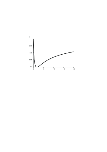
Figure 2: The spectral coefficient $\beta_{\nu}$ as the function of $x=\left(h\nu+cp\right)\left(E+cp\right)/m^{2}c^{4}$.

Now multiplying (27) on the number density of photons with the frequency $\nu$ and on the cross section we get the spectral force which accelerates the electron in the form

$$\mathbf{f}_{\nu}=\frac{\Delta\mathbf{p}}{\Delta t}=c\sigma_{T}N_{\nu}\frac{1}{c}\beta_{\nu}(p)h\nu\mathbf{n=}\frac{\sigma_{T}\beta_{\nu}(p)}{c}\mathbf{P}_{\nu}$$ (29)

where $\mathbf{P}_{\nu}$ is the spectral component of the Poynting vector $\mathbf{P_{\nu}=}\frac{c}{4\pi}\mathbf{E_{\nu}\times B}_{\nu}$ and $\sigma_{T}$ is the Thomson cross section. The total force is given by $\mathbf{F=}\int\mathbf{f}_{\nu}d\nu$.

It is important that the force is determined by the Poynting’s vector $\mathbf{P}_{\nu}$. In a quite (quasi-stationary or steady state) galaxy both the Poynting’s vector and the force have the potential character, i.e., they can be presented as $\mathbf{P_{\nu}=-\nabla}\Psi_{\nu}$. Non-stationary processes in active galactic nuclei may produce some additional acceleration, e.g., the stochastic Fermi acceleration, etc., which we do not discus here. For the quasi-stationary galaxy the Poynting’s theorem gives the discontinuity equation

$$div\mathbf{P_{\nu}=\ell}_{\nu}$$ (30)

where $\ell_{\nu}(x)$ is the spectral density of sources of radiation (stars, hot gas, dust, etc.) or the radiative capability of a unite volume in the galaxy. If the topology is simple, then sufficiently far from the galaxy we get

$$\mathbf{P_{\nu}=}\frac{M_{\nu}}{4\pi r^{2}}\mathbf{l,}$$ (31)

where $\mathbf{l=r/}r$, $\mathbf{r}$ is the distance from the center of the galaxy, and $M_{\nu}$ is the total spectral energy emitted by the galaxy in the unit time. Observations show that the intergalactic medium possesses a magnetic field Planck Collaboration (2016); Jones et. al. (2019). Therefore, the electron may have a closed trajectory. It is easy to verify that the total energy obtained by the electron from the galactic radiation during the cycle is exactly zero, i.e., $\oint\mathbf{f_{\nu}dl}\equiv 0$. This means that in the case when topology is simple, the only possible mechanism of the electron acceleration relates to high-energy non-stationary processes (jets, shock waves, supernovae explosions, active galactic nuclei, etc.).

The situation changes when the galaxy is accompanied with a wormhole. In the presence of the wormhole the Poynting’s field also admits non-trivial solutions of (30). For the sake of simplicity we consider the spherically symmetric (genus $n=0$) wormhole. For a more general wormhole the rough picture remains the same, at least from the qualitative standpoint. We point out that the genus $n\geq 1$ wormholes are more preferred from the astrophysical standpoint, since they may work as accelerators even in the case when a wormhole is not traversable (e.g., when the length of the trajectories which go through the throat are too big).

Indeed, the scattering of the radiation on the wormhole (e.g., see Kirillov & Savelova (2018, 2019)) produces an additional field in the dipole form

$$\delta\mathbf{P_{\nu}=}\frac{\delta M_{\nu}}{4\pi r_{-}^{2}}\mathbf{\mathbf{n}_{-}-}\frac{\delta M_{\nu}}{4\pi r_{+}^{2}}\mathbf{n}_{+}$$ (32)

where $\mathbf{n}_{\pm}=\mathbf{r}_{\pm}/r_{\pm}$, $\mathbf{r}_{\pm}=\mathbf{r}-\mathbf{x}_{\pm}$, $\mathbf{x}_{\pm}$ are positions of the wormhole entrances (we assume that $r_{+}\ll r_{-}$), $\delta M_{\nu}\simeq\frac{M_{\nu}\pi R^{2}}{4\pi r_{+}^{2}}$ is the portion of the spectral energy absorbed by the closest entrance into the wormhole throat and $R$ is the radius of the throat. If the wormhole possesses a magnetic field in the form (22), it forms a magnetic trap for the electron, while the Poynting’s vector field $\delta\mathbf{P_{\nu}}$ in form (32) forms the accelerating force which acts exactly along the magnetic lines. On every cycle the electron will gain the energy from radiation $A=\int A_{\nu}d\nu>0$, where $A_{\nu}=\oint\delta\mathbf{f_{\nu}dl}$, whose exact value depends on the length of the trajectory of the electron and on all the rest parameters of the wormhole (distance to the galaxy, throat size, etc.). Some part of this energy will be spent on the synchrotron radiation of electrons and, therefore, there is a competition between the acceleration produced by the galactic radiation and loss of energy on the reradiation. The reradiation can be accounted for by adding the standard force of the radiation friction.

VI Conclusions

In this manner we see that the system which consists of a galaxy and a wormhole endowed with a magnetic field works as an eternal accelerator. While particles have sufficiently small energy they are trapped and the system accelerates them. Particles of sufficiently high energies may leave the trap and contribute to the observed high-energy cosmic rays. The maximal possible energy which can be reached in such an accelerator depends on two basic factors.

The first factor is that due to the curvature of the magnetic lines electrons always have the component of the velocity which is orthogonal to the magnetic field. This causes the synchrotron radiation which gives the loss of the energy. For sufficiently high energies such a radiation becomes very strong and this restricts the maximal possible energy reached by such an accelerator (the exact value depends on all parameters of the accelerator). If the equilibrium between the acceleration and the loss of energy is reached, the wormhole starts to work simply as a generator of synchrotron radiation. Such objects should be directly seen on sky (the map of such sources is presented by Planck Collaboration (2016)). The problem of relating such sources to wormholes requires further and more rigorous investigation.

The second factor appears when such a limit is not reached (i.e., when the loss of the energy still does not exceed the obtained from the radiation value), then the absolute estimate of the threshold energy can be found as follows. The magnetic field reaches the maximal value at the throat and it is given by

$$B_{w}=\frac{Q}{R^{2}}.$$ (33)

Now consider the relation

$$V_{\perp}=r_{B}\omega_{B}=r_{B}\frac{eQ\gamma}{mcR^{2}}=r_{B}\frac{eB_{w}c}{E},$$ (34)

where $V_{\perp}$ is the component of the velocity transversal to the magnetic field (one may assume that $V_{\perp}\sim V_{\|}\sim c$), $\omega_{B}$ and $r_{B}$ are the Larmor’s frequency and radius respectively, $\gamma=(1-V^{2}/c^{2})^{1/2}$ is the relativistic factor, $e$ and $m$ are the electron charge and mass respectively, and $R$ is the size of the wormhole throat. To undergo the acceleration the electron should always get into the wormhole throat. This means that the Larmor’s radius should be smaller than the throat radius $r_{B}=c/(\omega_{B})=(cE)/(eB_{w}c)\leq R$. For ultra-relativistic particles this inequality determines the absolute threshold energy as

$$E\leq E_{th}=eB_{w}R.$$

Particles of higher energies cannot get into the throat and stop receiving the energy from the radiation. To find estimates we point out that the value $B_{w}$ can be related to the observed value in galaxies and clusters by the relation

$$B_{obs}\sim B_{w}(\frac{R}{L})^{2},$$

where $R$ is the radius of the throat and $L$ is the distance between the wormhole entrances. Then for the threshold energy we get the estimate energy as

$$E_{th}=eLB_{obs}\frac{L}{R}.$$

Now taking $R_{\bigodot}$ be the Sun radius, $L=L_{5}\times 5kpc$ (in dark matter models based on wormholes this corresponds to the scale when dark matter starts to show up Kirillov & Savelova (2008, 2011)), and $B_{obs}=B_{-9}nG=B_{-9}10^{-9}$ Gauss, we get the estimate

$$E_{th}\sim L^{2}_{5}B_{-9}\frac{R_{\bigodot}}{R}\times 10^{17}Gev.$$

We see that from the formal standpoint the threshold may reach and even exceed the Planckian value $\sim 10^{19}Gev$. However, for sufficiently small values of the throat radius we may expect that the matter density in the throat is very high. Therefore, the scattering on baryons in the throat will close such an accelerator for particles. In this sense the throat will be not traversable for charged particles. Consider now the estimate for torus-like (genus $n=1$) wormhole. In this case we may expect the value $R\sim 10^{-3}pc$ which gives the factor $R_{\bigodot}/R\sim 2.3\times 10^{-15}$ and the threshold energy estimate becomes

$$E_{th}\sim 2\L_{5}B_{-9}\times 100Gev.$$

This is already close to the reported in DAMPE Collaboration (2017) value for the break energy $E_{b}=(9.14\pm 0.98)100$Gev.

The intensity of the flow of high-energy particles leaving such an accelerator is determined by the luminosity of the galaxy, the distance between the wormhole and the galactic center, and the cross-section of the wormhole which has the order $\sim\pi R^{2}$.

In conclusion we point out that if we have two such wormholes near the same galaxy (or even in two different galaxies), then they should produce different contributions to the high-energy cosmic-ray spectrum depending on parameters of the wormholes, activity of the galaxy, etc. This allows us to interpret the break of the high-energy spectrum observed in DAMPE Collaboration (2017) as contributions from different wormholes. In general wormholes have different threshold energies. The break indicates that at least one of wormholes has the threshold energy $E_{th}\simeq E_{b}$. This however still does not allow us to derive rigorous estimates to all wormhole parameters $L$, $R$, and $B_{w}$.

References

- Pierre Auger Collaboration (2010) Abraham J. et al. (Pierre Auger Collaboration) Measurement of the Depth of Maximum of Extensive Air Showers above eV , Phys. Rev. Lett. 104, 091101 (2010).
- DAMPE Collaboration (2017) DAMPE Collaboration: Direct detection of a break in the teraelectronvolt cosmic-ray spectrum of electrons and positrons, Nature 552, 24475 (2017).
- Eichmann et. al. (2018) Eichmann B., et. al., Ultra-high-energy cosmic rays from radio galaxies, J. Cosmol. Astroparticle Physics 02 2018, 036 (2018).
- Hillas (1984) Hillas A.M., The Origin of Ultra-High-Energy Cosmic Rays, Ann. Rev. Astron. Astrophys. 22, 425 (1984).
- Feng (2010) Feng J.L., Dark Matter Candidates from Particle Physics and Methods of Detection, Annu. Rev. Astron. Astrophys. 48, 495 (2010).
- Grib & Pavlov (2009) Grib A.A., Pavlov Yu.V., Active Galactic Nuclei and Transformation of Dark Matter into Visible Matter, Gravitation and Cosmology 15, 44 (2009).
- Belotsky, et al. (2014) Belotsky K., Khlopov M., Laletin M., Kouvaris C., Decaying Dark Atom Constituents and Cosmic Positron Excess, Advances in High Energy Physics, 2014 214258 (2014).
- Belotsky, et al. (2015) Belotsky K., Khlopov M., Laletin M., Kouvaris C., High-Energy Positrons and Gamma Radiation from Decaying Constituents of a Two-component Dark Atom Model, Int. J. Mod. Phys. D 24 1545004 (2015).
- Visser (1996) Visser M., Lorentzian wormholes, Springer-Verlag, New-York, Inc. (1996).
- Hochberg et al. (1997) Hochberg D., Popov A., Sushkov S.V., Self-Consistent Wormhole Solutions of Semiclassical Gravity, Phys. Rev. Lett. 78, 2050 (1997).
- Harko et al. (2013) Harko T., Lobo F.S.N., Mak M.K., Sushkov S.V., Modified-Gravity Wormholes without Exotic Matter, Phys. Rev. D 87, 067504 (2013).
- Myrzakulov et al. (2016) R. Myrzakulov, L. Sebastiani, S. Vagnozzi, and S. Zerbini, Static spherically symmetric solutions in mimetic gravity: rotation curves & wormholes, Class. Quant. Grav. 33 125005 (2016).
- Lobo (2017) Lobo, F.S.N., Wormholes, Warp Drives and Energy Conditions, Fundam. Theor. Phys. 189 (2017).
- Arellano & Lobo (2006) Arellano A. V. B., Lobo, F.S.N., Evolving wormhole geometries within nonlinear electrodynamics, Class. Quant. Grav. 23, 5811 (2006).
- Kirillov & Savelova (2016) Kirillov A.A. & Savelova E.P., Cosmological wormholes, Int. J. Mod. Phys. D 25, 1650075 (2016).
- Bronnikov et al. (2013) Bronnikov K.A., Krechet V.G., and Lemos J.P.S., Rotating cylindrical wormholes, Phys. Rev. D 87, 084060 (2013).
- Bronnikov & Lemos (2009) Bronnikov K.A. & Lemos J.P.S., Cylindrical wormholes, Phys. Rev. D 79, 104019 (2009).
- Bronnikov & Krechet (2019a) Bronnikov K.A.& Krechet V.G., Potentially observable cylindrical wormholes without exotic matter in general relativity, Phys. Rev. D 99, 084051 (2019).
- Bronnikov et al. (2019b) Bronnikov K.A., Bolokhov S.V., and Skvortsova M.V., Cylindrical wormholes: a search for viable phantom-free models in GR, Int. J. Mod. Phys. D 28, 1941008 (2019).
- Planck Collaboration (2016) Planck Collaboration: Planck 2015 results XIII. Cosmological parameters, Astron. Astrophys. 594, A13 (2016).
- Geroch (1967) Geroch R.P., Topology in general relativity, J. Math. Phys. 8, 782 (1967).
- Fomenko (1999) Fomenko A.T., 1999, Differential geometry and topology. Additional chapters, Izhevsk, ”Regular and chaotic dynamics” [in russian] www.rcd.com.ru
- Hempel (1976) Hempel J., 1976, Topology of 3-Manifolds, Princeton University Press.
- Planck Collaboration (2018) Planck Collaboration: Planck 2018 results. VI. Cosmological parameters, arXiv:1807.06209
- Jones et. al. (2019) Jones T.J. et. al., SOFIA Far-infrared Imaging Polarimetry of M82 and NGC 253: Exploring the Supergalactic Wind, Astr. Journ. Lett. 870, L9 (2019)
- Kirillov & Savelova (2008) Kirillov A.A. & Savelova E.P., Dark matter from a gas of wormholes, Phys. Lett. B 660, 93 (2008).
- Kirillov & Savelova (2011) Kirillov A.A. & Savelova E.P., Density perturbations in a gas of wormholes, Mon. Not. RAS 412, 1710 (2011).
- Kirillov & Savelova (2018) Kirillov A.A. & Savelova E.P., Effects of Scattering of Radiation on Wormholes, Universe 4, 35 (2018).
- Kirillov & Savelova (2019) Kirillov A.A. & Savelova E.P., On distortion of the background radiation spectrum by wormholes: kinematic Sunyaev-Zel’dovich effect, Astr. Sp. Sc. 364, 1 (2019).
- Lifshitz (1946) Lifshitz E., On the gravitational stability of the expanding universe, J. Phys. (USSR) 10, 116–129 (1946), republication in: Gen. Relativ. Gravit. 49:18 (2017).
- Mukhanov (2005) Mukhanov V.F. Physical foundations of cosmology (CUP, 2005)(ISBN 0521563984) p.442
- Bronnikov (2018) Bronnikov K. A., Nonlinear electrodynamics, regular black holes and wormholes, Int. J. Mod. Phys. D 27 1841005 (2018).
- Subramanian (2016) Subramanian K., The origin, evolution and signatures of primordial magnetic fields, Rep. Prog. Phys. 79, 076901 (2016).
- Bronnikov (1973) Bronnikov K. A., Scalar-Tensor Theory and Scalar Charge, Acta Physica Polonica  4, 251(1973).
- Ellis (1973) Ellis H. G., Ether flow through a drainhole – a particle model in general relativity, J. Math. Phys. 14, 104 (1973).