Energy Efficiency Fairness Beamforming Designs for MISO NOMA Systems

Abstract

In this paper, we propose two beamforming designs for a multiple-input single-output non-orthogonal multiple access system considering the energy efficiency (EE) fairness between users. In particular, two quantitative fairness-based designs are developed to maintain fairness between the users in terms of achieved EE: max-min energy efficiency (MMEE) and proportional fairness (PF) designs. While the MMEE-based design aims to maximize the minimum EE of the users in the system, the PF-based design aims to seek a good balance between the global energy efficiency of the system and the EE fairness between the users. Detailed simulation results indicate that our proposed designs offer many-fold EE improvements over the existing energy-efficient beamforming designs.

I Introduction

Non-orthogonal multiple access (NOMA) has been recently envisioned as a promising multiple access technique to be used in future wireless networks for addressing the issue of low spectral efficiency in conventional orthogonal multiple access (OMA) and to provide massive connectivity [1]. In this novel multiple access scheme, multiple users share the same orthogonal resources (i.e., time, frequency and spreading codes) by exploiting power-domain multiplexing [2]. In particular, superposition coding (SC) is employed at the transmitter to multiplex the signals of multiple users in the power domain [2], and then, the successive interference cancellation (SIC) technique is used at the receiving ends to eliminate inter-user interference and to decode the signals [3, 4].

To facilitate a practical implementation of NOMA in dense networks, and to further improve the spectral efficiency [5], NOMA is incorporated with multiple antenna techniques to exploit their additional degrees of freedom offered by the different spatial multiplexing schemes [6] [7]. As such, NOMA has the potential capabilities to support the extensive deployment of the Internet-of-Things (IoT) in fifth generation (5G) and beyond wireless networks [3]. However, the limitation of the available power resources becomes one of the major challenges in the development of future technologies. This should be taken into account in the design of new transmission techniques [8]. The energy efficiency (EE), defined as the ratio between the achieved sum rate in the system and the total power consumption to achieve those rates at users [9], is a useful metric for comparing and characterizing different schemes, such as beamforming designs. Furthermore, the EE can also help to strike a good balance between the achieved rate in the system and the total power consumption [10]. Note that the terms EE and global energy efficiency (GEE) carry the same meaning in this paper. In particular, GEE considers the overall EE of the system without taking the performance of the individual users into account. Hence, the users with weaker channel conditions (i.e., cell-edge users) might achieve a very low EE compared to those users with stronger channel conditions (near users). To overcome such a fairness issue among the users, the transmitter should be able to incorporate the performance of the individual users in the design rather than optimizing the GEE of the system. Furthermore, while there is no unique definition for fairness, this could be generally defined in terms of allocating the resources between the users to provide a reasonable quality-of-service at all of them [11].

Motivated by the prominence of the fairness in terms of the achieved EE for each user, we consider energy-efficient fairness-based beamforming designs for a multiple-input single-output (MISO) NOMA system. The beamforming design with GEE is considered for a MISO NOMA system in [9]. In particular, we present two fairness based designs in this paper, namely, max-min energy efficiency (MMEE) and proportional fairness (PF) based designs. First, MMEE is considered as the bottleneck fairness design [12] [13]. As such, MMEE is achieved if any performance increment in the EE of the $i^{th}$ user (EE_i) causes a deterioration of the EE of the $j^{th}$ user (i.e., EE_j) which already has lower performance [14]. Despite the fact that the MMEE design aims to achieve the same EE for all users by maximizing the minimum EE of a user, the fairness in this design comes at the cost of GEE degradation. Therefore, we consider another approach, namely the PF-based design, which has the capability to finding a good balance between GEE and achieved EE for each user [12]. Assume that a design achieves an EE of EE_i at the $i^{th}$ user in a system with $K$ users by allocating an amount of $\Gamma_{i}$ resources. Then, the resource allocation $\{\Gamma^{*}_{i}\}_{i=1}^{K}$ is considered to be a proportionally fair if the following condition holds for any other feasible resource allocation $\{\Gamma_{i}\}_{i=1}^{K}$ [11]:

$$\sum_{i=1}^{K}\frac{\text{EE}_{i}-\text{EE}^{*}_{i}}{\text{EE}^{*}_{i}}\leq 0,$$ (1)

where $\text{EE}_{i}^{*}$ corresponds to $\Gamma^{*}_{i}$. It is worth mentioning that the condition in (1) can be satisfied through determining the feasible set $\{\Gamma^{*}_{i}\}_{i=1}^{K}$ that maximizes $\sum_{i=1}^{K}\log(\text{EE}_{i})$ [15]. In this paper, we formulate fairness-based beamforming designs (i.e., MMEE and PF) for a MISO NOMA system with total power constraint at the base station (BS) and minimum rate requirement at each user. However, these optimization problems are non-convex in nature in terms of beamforming vectors. Hence, we employ the sequential convex approximation (SCA) technique to tackle the non-convexity issues associated with these optimization problems. In addition, we demonstrate the effectiveness of the proposed designs by evaluating and comparing their performances with that of the existing beamforming designs in the literature.

The rest of the paper is organized as follows. In Section II, the system model and problem formulations are introduced. Section III presents the SCA technique as an effective approach to solve the original non-convex optimization problems. To validate the performance of the proposed designs, numerical results are provided in Section IV. Finally, conclusions of this work are presented in Section V.

Notations

We use lower case boldface letters for vectors and upper case boldface letters for matrices. $(\cdot)^{H}$ denotes complex conjugate transpose. $\Re(\cdot)$ and $\Im(\cdot)$ stand for real and imaginary parts of a complex number, respectively. The symbols $\mathbb{C}^{N}$ and $\mathbb{R}^{N}$ denote $N$-dimensional complex and real space, respectively. $||\cdot||_{2}$ and $|\cdot|$ represent the Euclidean norm of a vector and absolute value of a complex number, respectively.

II System Model And Problem Formulations

A) System Model

We consider a downlink transmission of a MISO NOMA system, in which a BS equipped with $N$ multiple antennas communicates simultaneously with $K$ single-antenna users. It is assumed that BS has the perfect channel state information of each user. The BS encodes the message of the $i^{th}$ user ($s_{i}$) by scaling the message using linear precoding vector (beamforming vector) $\mathbf{w}_{i}$ $\in$ $\mathbb{C}^{N\times 1}$. Thus, the transmitted signal $\mathbf{x}\in\mathbb{C}^{N\times 1}$ from the BS can be written as

$$\mathbf{x}=\sum_{i=1}^{K}\mathbf{w}_{i}s_{i}.$$ (2)

The received signal at the $i^{th}$ user ($U_{i})$ can be expressed as

$$y_{i}=\sum_{j=1}^{K}\mathbf{h}_{i}^{H}\mathbf{w}_{j}s_{j}+n_{i},\forall i\in\mathcal{K}\overset{\bigtriangleup}{=}\{1,2,3,\cdots,K\},$$ (3)

where $\mathbf{h}_{i}$ $\in$ $\mathbb{C}^{N\times 1}$ represents the channel vector between $U_{i}$ and BS. The channel coefficients are modeled as $\mathbf{h}_{i}=\sqrt{d_{i}^{-\kappa}}\mathbf{v}_{i}$, where $\kappa$ and $d_{i}$ are the path loss exponent and the distance between $U_{i}$ and BS in meter, respectively. Furthermore, $\mathbf{v}_{i}$ and $n_{i}$ represent the small scale fading and the zero-mean circularly symmetric complex additive white Gaussian noise with variance $\sigma_{i}^{2}$, respectively. In downlink transmission of a NOMA system, the stronger users employ SIC by firstly decoding and eliminating the interference from the signals of the users with weaker channel conditions, and then detect their own signals [2]. Here, we assume that $U_{1}$ is the strongest user with the most favourable channel condition, whereas $U_{K}$ is the weakest user. In particular, the users are ordered based on their channel strengths such that

$$||\mathbf{h}_{1}||^{2}\geq||\mathbf{h}_{2}||^{2}\geq\cdots\geq||\mathbf{h}_{K}||^{2}.$$ (4)

Based on this user ordering, the received signal at $U_{i}$ after successfully eliminating the interference from the weaker users through SIC can be written as

$$\overset{\sim}{y_{i}}=\mathbf{h}_{i}^{H}\mathbf{w}_{i}s_{i}+\sum_{j=1}^{i-1}\mathbf{h}_{i}^{H}\mathbf{w}_{j}s_{j}+n_{i},\forall i\in\mathcal{K}.$$ (5)

In particular, the message intended for the $i^{th}$ user is decoded at the stronger user $U_{k}$ (i.e., $k\leq i$) with the following signal-to-interference plus noise ratio (SINR):

$$\text{SINR}^{(i)}_{k}=\frac{|\mathbf{h}_{k}^{H}\mathbf{w}_{i}|^{2}}{\sum_{j=1}^{i-1}|\mathbf{h}_{k}^{H}\mathbf{w}_{j}|^{2}+\sigma_{k}^{2}},\quad\forall i\in\mathcal{K},k\leq i.$$ (6)

Note that the signal intended for $U_{i}$ could not be correctly decoded unless the SINR of the corresponding signal is larger than a certain threshold ($\eta_{i}^{min}$). This explicitly means that the SINR of decoding the $i^{th}$ user signal at the stronger users should be greater than this threshold (i.e., $\eta_{i}^{min}$). Therefore, the SINR of the $i^{th}$ user can be defined as in [16]

$$\text{SINR}_{i}=\text{minimum}({\text{SINR}^{(i)}_{1},\cdots,\text{SINR}^{(i)}_{i}}),\forall i\in\mathcal{K}.$$ (7)

Hence, the achieved rate at $U_{i}$ can be expressed as

$$R_{i}=B_{w}\log_{2}(1+\text{SINR}_{i})\forall i\in\mathcal{K},$$ (8)

where $B_{w}$ denotes the available bandwidth for the transmission. For notational simplicity, we select $B_{w}$ to be 1. To ensure that the power assigned to each user in the system is inversely proportional to its channel strengths [17], and to allow SIC to be successfully implemented at the strong users [16], the following conditions should be considered in the design:

$$|\mathbf{h}_{i}^{H}\mathbf{w}_{K}|^{2}\geq\cdots\geq|\mathbf{h}_{i}^{H}\mathbf{w}_{1}|^{2},\forall i\in\mathcal{K}.$$ (9)

In this MISO NOMA system, the achieved EE at the $i^{th}$ user (i.e., EE_i) is defined as the ratio between the achieved rate at $U_{i}$ and the consumed power at the BS to achieve this rate [10], which can be expressed as

$$\text{EE}_{i}=\frac{R_{i}}{\frac{1}{\epsilon_{0}}P_{i}+P_{l,i}},\forall i\in\mathcal{K},$$ (10)

where $P_{i}$ and $P_{l,i}$ denote the transmit power allocated to $U_{i}$ and the corresponding power losses associated with that user at the BS, respectively. Note that $P_{i}=||\mathbf{w}_{i}||_{2}^{2},$ and $\epsilon_{0}$ represents the efficiency of the amplifiers at the BS. Furthermore, the GEE of the system can be defined as

$$\text{GEE}=\frac{\sum_{j=1}^{K}R_{j}}{\frac{1}{\epsilon_{0}}P+P_{l}},$$ (11)

where $P_{l}$ represents the total power losses at the BS and $P$ denotes the total transmit power required for data transmission from the BS. The available total transmit power at the BS is limited to $P_{ava}$, which can be represented by the following constraint:

$$P=\sum_{i=1}^{K}P_{i}\leq P_{ava}.$$ (12)

In the conventional GEE maximization (GEE-Max)-based design, the beamforming vectors are determined by maximizing the GEE under the SIC constraints in (9), and with a minimum rate requirement at each user ($R_{i}^{min}$). This minimum rate requirement at the $i^{th}$ user can be imposed by the following constraint:

$$R_{i}\geq R_{i}^{min},\forall i\in\mathcal{K}.$$ (13)

The GEE-Max problem can be formulated as

$$OP_{GEE}\!: \underset{\{\mathbf{w}_{i}\}_{i=1}^{K}}{\text{max }}$$ GEE (14a)

s.t. $$\!\!\!\!\!\!\!\!\!\!\!\!\!\!\!\!\!\!\!\!\!\!\!\!\!(\ref{channels}),(\ref{power1}),(\ref{mon}).$$ (14b)

This GEE-Max problem $OP_{GEE}$ is solved in our previous work using the SCA technique and the Dinkelbach’s algorithm  [9]. In this paper, we consider the fairness-based beamforming designs, which are discussed in detail in the following subsection.

B) Problem Formulations

In this subsection, two fairness-based beamforming designs are proposed, namely MMEE and PF designs.

B)1 Max-min energy efficiency (MMEE)

Unlike the GEE-Max-based design in $OP_{GEE}$, the MMEE design aims for maximizing the minimum EE of users in the system while satisfying the associated constraints [18]. In particular, the MMEE achieves its ideal solution while all the users experience the same EE. However, this is not a universal condition owing to the minimum rate and SIC constraints. The MMEE-based design for the MISO NOMA system is formulated as follows:

$$OP_{1}: \underset{\{\mathbf{w}_{i}\}_{i=1}^{K}}{\text{max}} \text{min\leavevmode\nobreak\ }\{\text{EE}_{1},\text{EE}_{2},\cdots,\text{EE}_{K}\}$$ (15a)

s.t. $$(\ref{channels}),(\ref{power1}),(\ref{mon}).$$ (15b)

This max-min problem is not convex due to the non-convex objective function in (15a), the SIC constraint in (9), and the minimum rate requirement in (13). Therefore, the solution to the problem $OP_{1}$ cannot easily be determined through existing convex optimization techniques [19].

B)2 Proportional Fairness (PF)

Next, we consider a PF-based design to seek a good balance between the beamforming designs without any fairness and with ideal fairness conditions, namely GEE-Max design and MMEE design, respectively. The PF design can be defined into the following optimization framework [11]:

$$OP_{2}: \underset{\{\mathbf{w}_{i}\}_{i=1}^{K}}{\text{max}} \!\!\!\!\!\!\!\!\!\!\!\!\!\!\!\!\!\!\!\sum_{i=1}^{K}\log(\text{EE}_{i})$$ (16a)

s.t. $$\!\!\!\!\!\!\!\!\!\!\!\!\!\!\!\!\!\!\!(\ref{channels}),(\ref{power1}),(\ref{mon}).$$ (16b)

The solutions for the non-convex problems $OP_{1}$ and $OP_{2}$ are presented in the following section.

III Proposed methodology

In this section, we exploit different techniques to convert the original non-convex functions in $OP_{1}$ and $OP_{2}$ to convex ones. In particular, the SCA technique is used to approximate those functions into linear convex functions [9, 20, 21]. In the SCA technique, a set of convex lower bounds are defined with a number of slack variables to approximate the non-convex objective function or constraint [21] into a convex objective function. As such, the SCA will be implemented to handle the non-convexity of (15) and (16).

Non-convex constraints in $OP_{1}$ and $OP_{2}$

As both $OP_{1}$ and $OP_{2}$ share the same constraints, we first show how to formulate the non-convex constraints in (15) and (16). Without loss of generality, the minimum rate constraint in (13) can be equivalently expressed in terms of SINR as

$$\frac{|\mathbf{h}_{k}^{H}\mathbf{w}_{i}|^{2}}{\sum_{j=1}^{i-1}|\mathbf{h}_{k}^{H}\mathbf{w}_{j}|^{2}+\sigma_{k}^{2}}\geq\eta_{i}^{min},i\in\mathcal{K},k\leq i,$$ (17)

where $\eta_{i}^{min}=2^{R_{i}^{min}}-1$. Furthermore, this constraint can be easily reformulated into a second order cone (SOC) as [22]:

$$\frac{1}{\sqrt{\eta_{i}^{min}}}\Re(\mathbf{h}_{k}^{H}\mathbf{w}_{i})\geq\\ ||[\mathbf{h}_{k}^{H}\mathbf{w}_{1}\leavevmode\nobreak\ \mathbf{h}_{k}^{H}\mathbf{w}_{2}\leavevmode\nobreak\ \cdots\leavevmode\nobreak\ \mathbf{h}_{k}^{H}\mathbf{w}_{i-1}\leavevmode\nobreak\ \sigma_{k}]^{T}||_{2},i\in\mathcal{K},k\leq i.$$ (18)

Next, the non-convexity of the SIC constraint in (9) is handled by using minorization-maximization algorithm (MMA) [16] [23]. In particular, the non-convex function is approximated by linear terms at a given set of values using convex-concave procedure. Furthermore, we use the first-order Taylor series expansion to approximate the constraint in (9), where each term in the inequality is replaced by a lower bounded linear function $f_{k,j}$ such that $|\mathbf{h}_{k}^{H}\mathbf{w}_{j}|^{2}\geq f_{k,j}$, where

$$f_{k,j}=||[\Re{(\mathbf{h}_{k}^{H}\mathbf{w}_{j}^{(n)})}\leavevmode\nobreak\ \Im{(\mathbf{h}_{k}^{H}\mathbf{w}_{j}^{(n)})}]||^{2}_{2}\\ +2[\Re{(\mathbf{h}_{k}^{H}\mathbf{w}_{j}^{(n)})}\leavevmode\nobreak\ \Im{(\mathbf{h}_{k}^{H}\mathbf{w}_{j}^{(n)})}]^{T}[(\Re{(\mathbf{h}_{k}^{H}\mathbf{w}_{j})}\\ -\Re{(\mathbf{h}_{k}^{H}\mathbf{w}_{j}^{(n)})})\leavevmode\nobreak\ (\Im{(\mathbf{h}_{k}^{H}\mathbf{w}_{j})}-\Im{(\mathbf{h}_{k}^{H}\mathbf{w}_{j}^{(n)})})]^{T},$$ (19)

where $\mathbf{w}_{i}^{(n)}$ represents the approximation of $\mathbf{w}_{i}$ at the $n^{th}$ iteration. Note that the function in (19) is linear in terms of $\mathbf{w}_{i}$. Based on this approximation, the non-convex constraint in (9) can be approximated as the following convex constraint:

$$f_{i,K}\geq\cdots\geq f_{i,1},\forall i\in\mathcal{K}.$$ (20)

To this end, we have approximated the non-convex constraints in the original optimization problems $OP_{1}$ and $OP_{2}$ by convex constraints.

MMEE Design

In the following, we transform the original non-convex objective function of the MMEE design in $OP_{1}$ by introducing a new slack variable $\alpha$ as

$$\text{min\leavevmode\nobreak\ }\{\text{EE}_{1},\text{EE}_{2},\cdots,\text{EE}_{K}\}\geq\alpha.$$

Without loss of generality, the optimization problem in $OP_{1}$ can be equivalently written as

$$\overset{\sim}{OP_{1}}\!\!: \underset{\{\mathbf{w}_{i}\}_{i=1}^{K}}{\text{max }} \!\!\!\!\!\!\!\!\!\!\!\!\!\!\!\alpha$$ (21a)

s.t. $$\!\!\!\!\!\!\!\!\!\!\!\!\!\!\!\!\!(\ref{channeld}),(\ref{power1}),(\ref{const112}),$$ (21b)

$$\!\!\!\!\!\!\!\!\!\!\!\!\!\!\!\!\!\text{EE}_{i}\geq\alpha,i\in\mathcal{K}.$$ (21c)

To handle the non-convexity of the constraint in (21c), we re-formulate this with a new slack variable $\beta_{i}$ into two sets of constraints as follows:

$$R_{i}\geq{\alpha\beta_{i}^{2}},\forall i\in\mathcal{K},k\leq i,$$ (22a)

$$\frac{1}{\epsilon_{0}}||\mathbf{w}_{i}||^{2}_{2}+P_{l,i}\leq{\beta_{i}^{2}},\forall i\in\mathcal{K}.$$ (22b)

Following a similar formulation as in (18), the constraint in (22b) can be cast as the following standard convex SOC:

$$\beta_{i}\geq||[\frac{\mathbf{w}_{i}}{\sqrt{\epsilon_{0}}}\leavevmode\nobreak\ \sqrt{P_{l,i}}]^{T}||_{2},\quad\forall i\in\mathcal{K}.$$ (23)

Furthermore, we introduce a new set of slack variables $\delta_{i}$ and $\tau_{i}$ to approximate the non-convex constraint in (22a) as

$$\log(1+\text{SINR}_{k}^{(i)})\geq\delta_{i},\forall i\in\mathcal{K},k\leq i,$$ (24a)

$$(1+\text{SINR}_{k}^{(i)})\geq\tau_{i},\forall i\in\mathcal{K},k\leq i,$$ (24b)

which can be equivalently represented as the following set of constraints:

$$(\ref{eqn1s1})\Leftrightarrow \frac{|\mathbf{h}_{k}^{H}\mathbf{w}_{i}|^{2}}{\sum_{j=1}^{i-1}|\mathbf{h}_{k}^{H}\mathbf{w}_{j}|^{2}+\sigma_{k}^{2}}\geq\tau_{i}-1,k\leq i,$$ (25a)

$$(\ref{eqn1s1})\Leftrightarrow \tau_{i}\geq 2^{\delta_{i}},\quad\forall i\in\mathcal{K}$$ (25b)

$$(\ref{eqn1s1})\Leftrightarrow \delta_{i}\geq{\alpha\beta_{i}^{2}},i\in\mathcal{K}.$$ (25c)

The non-convexity of the constraint in (25a) is handled by incorporating a new slack variable $\rho_{i,k}^{2}$ and splitting it into the following two sets of constraints:

$$|\mathbf{h}_{k}^{H}\mathbf{w}_{i}|^{2}\geq(\tau_{i}-1)\rho_{i,k}^{2},\forall i\in\mathcal{K},k\leq i,$$ (26a)

$$\rho_{i,k}^{2}\geq{\sum_{j=1}^{i-1}|\mathbf{h}_{k}^{H}\mathbf{w}_{j}|^{2}+\sigma_{k}^{2}},\forall i\in\mathcal{K},k\leq i.$$ (26b)

Following the same approach in (18), the constraint in (26b) can be transformed into a standard convex SOC constraint as

$$\rho_{i,k}\geq||[\mathbf{h}_{k}^{H}\mathbf{w}_{1}\leavevmode\nobreak\ \mathbf{h}_{k}^{H}\mathbf{w}_{2}\leavevmode\nobreak\ \cdots\leavevmode\nobreak\ \mathbf{h}_{k}^{H}\mathbf{w}_{i-1}\leavevmode\nobreak\ \sigma_{k}]^{T}||_{2},\\ \forall i\in\mathcal{K},k\leq i.$$ (27)

Furthermore, the constraint in (26a) can be represented as the following convex constraint:

$$\Re({\mathbf{h}_{k}^{H}\mathbf{w}_{i}})\geq\\ \sqrt{(\tau_{i}^{{(n)}}-1)}\rho_{i,k}^{{(n)}}+0.5\frac{1}{\sqrt{(\tau_{i}^{{(n)}}-1)}}\rho_{i,k}^{{(n)}}(\tau_{i}-\tau_{i}^{{(n)}})+\\ \sqrt{(\tau_{i}^{{(n)}}-1)}(\rho_{i,k}-\rho_{i,k}^{{(n)}}),\forall i\in\mathcal{K},k\leq i.$$ (28)

Finally, we employ the first-order Taylor series expansion to approximate the right hand-side of (25c) as follows:

$$\delta_{i}\geq{\alpha^{(n)}(\beta_{i}^{2})^{(n)}}+(\beta_{i}^{2})^{(n)}(\alpha-\alpha^{(n)})\\ +2\beta_{i}^{(n)}\alpha^{(n)}(\beta_{i}-\beta_{i}^{(n)}),\quad i\in\mathcal{K}.$$ (29)

After introducing these multiple slack variables, the original non-convex MMEE optimization problem $OP_{1}$ is approximated as the following optimization problem:

$$\overset{\approx}{OP_{1}}\!\!\!:\leavevmode\nobreak\ \leavevmode\nobreak\ \underset{\chi}{\text{max }} \!\!\!\!\!\!\!\!\!\!\!\!\!\alpha$$ (30a)

s.t. $$\!\!\!\!\!\!\!\!\!\!\!\!\!(\ref{kog}),$$ (30b)

$$\!\!\!\!\!\!\!\!\!\!\!\!\!(\ref{fg}),(\ref{sec}),(\ref{dsd}),(\ref{cuma}),(\ref{najw}),$$ (30c)

where $\chi$ includes all the optimization variables involved in the MMEE problem: $\chi\overset{\bigtriangleup}{=}\{\mathbf{w}_{k},\rho_{i,k},\tau_{i},\beta_{i},\delta_{i},\alpha\}_{i=1}^{K}$.

PF Design

Next, we consider the PF maximization problem $OP_{2}$. The non-convex constraints in $OP_{2}$ have been already reformulated as convex constraints in previous subsection. However, the non-convexity of the objective function in $OP_{2}$ can be tackled by introducing new slack variables $\mu_{i}$ and $\varsigma_{i}$ as

$$\log\text{EE}_{i}\geq{\varsigma_{i}},\forall i\in\mathcal{K},$$ (31a)

$$\text{EE}_{i}\geq\mu_{i},\forall i\in\mathcal{K}.$$ (31b)

With these new slack variables, $OP_{2}$ can be equivalently expressed as

$$\overset{\sim}{OP_{2}}\!\!: \underset{\{\mathbf{w}_{i}\}_{i=1}^{K}}{\text{max }} \!\!\!\!\!\!\!\!\!\!\!\!\!\!\!\!\!\!\!\!\sum_{i=1}^{K}\varsigma_{i}$$ (32a)

s.t. $$\!\!\!\!\!\!\!\!\!\!\!\!\!\!\!\!\!\!\!\!\mu_{i}\geq 2^{\varsigma_{i}},i\in\mathcal{K},$$ (32b)

$$\!\!\!\!\!\!\!\!\!\!\!\!\!\!\!\!\!\!\!\!\text{EE}_{i}\geq\mu_{i},i\in\mathcal{K},$$ (32c)

$$\!\!\!\!\!\!\!\!\!\!\!\!\!\!\!\!\!\!\!\!(\ref{kog}).$$ (32d)

Without loss of generality, we can convert the non-convex constraint in (32c) to a convex one by using the same approach as in (21c). This could be implemented by replacing $\alpha$ in (21c) by $\mu_{i}$, and then applying the corresponding approximations. Hence, the problem $\overset{\sim}{OP_{2}}$ can be written in a convex form as

$$\overset{\approx}{OP_{2}}\!\!:\leavevmode\nobreak\ \leavevmode\nobreak\ \underset{\varphi}{\text{max}} \sum_{i=1}^{K}\varsigma_{i}$$ (33a)

s.t. $$(\ref{kog}),$$ (33b)

$$\mu_{i}\geq 2^{\varsigma_{i}},i\in\mathcal{K},$$ (33c)

$$(\ref{alam}),$$ (33d)

where $\varphi$ consists of all the optimization variables: $\varphi\overset{\bigtriangleup}{=}\{\varsigma_{i},\mathbf{w}_{i},\rho_{i,k},\tau_{i},\beta_{i},\delta_{i},\mu_{i}\}_{i=1}^{K}$. Note that $\alpha$ is replaced by $\mu_{i}$ at all constraints in (33d).
It is worth noting that the solutions of $\overset{\approx}{OP_{1}}$ and $\overset{\approx}{OP_{2}}$ depend on the appropriate selection of the initial parameters: $\chi^{(0)}$ and $\varphi^{(0)}$. These initial parameters are chosen by determining the beamforming vectors ($\{\mathbf{w}_{i}^{(0)}\}_{i=1}^{K}$) that minimize the total transmit power (i.e., $P=\sum_{i=1}^{K}||\mathbf{w}_{i}||_{2}^{2}$) subject to the minimum SINR constraint in (13) and the SIC constraint in (9) [24]. Then, all initial parameters (i.e., $\chi^{(0)}$ and $\varphi^{(0)}$) are evaluated by replacing the inequality with equality at each constraint.

On the other hand, it is obvious that the solutions of $\overset{\approx}{OP_{1}}$ and $\overset{\approx}{OP_{2}}$ can be iteratively obtained. This iterative approach can be terminated by comparing the difference of the objective values at two successive iterations against a predefined threshold $\varepsilon$. We summarize the developed algorithms to determine the solutions of the original MMEE and PF designs in Algorithm 1 and Algorithm 2, respectively.

Algorithm 1: MMEE design using SCA

Step 1: Initialization of $\chi^{(0)}$

Step 2: Repeat

1. Solve the optimization problem $\overset{\approx}{OP_{1}}$ in (30).

2. Update $\chi^{(n)}$ .

Step 3: Until required accuracy is achieved.

Algorithm 2: PF design using SCA

Step 1: Initialization of $\varphi^{(0)}$

Step 2: Repeat

1. Solve the optimization problem $\overset{\approx}{OP_{2}}$ in (33).

2. Update $\varphi^{(n)}$ .

Step 3: Until required accuracy is achieved.

IV Numerical Results

To demonstrate the effectiveness of the two proposed designs, namely the MMEE- and PF-based designs, we perform a number of detailed simulations. In presenting the results, we use the conventional GEE-Max-based design as baseline. In our simulation studies, we consider a downlink transmission where a BS equipped with three transmit antennas ($N=3$) sends signals to three users ($K=3$). It is assumed that the users are located at the distance of 1, 5.5, and 25 meters from the BS, respectively. The relevant parameters of the simulation setup are shown in Table I.

Table I: Parameters used in simulations.

Param.	Description	Value(s)
$\kappa$	Path loss exponent	$2.0$
$\sigma_{i}^{2}$	Noise variance for user $i$	$2.0$
$\eta_{i}^{min}$	SINR threshold	$10^{-3}$
$P_{l,i}$	Power loss at the BS	$45$ dBm
$\epsilon_{0}$	Amplifier efficiency at BS	$0.65$
$B_{w}$	Available bandwidth	$1$ MHz
$\varepsilon$	Thresholds for the algorithms	$0.001$
$\mathbf{v}_{i}$	Small scale fading	Rayleigh fading

In addition to these parameter settings, we define the normalized transmit power (TX-SNR) in dB as TX-SNR (dB)= $10{\log}_{10}\frac{P_{ava}}{\sigma_{i}^{2}}$. It is worth mentioning that all simulations in this section are carried out using the CVX toolbox.

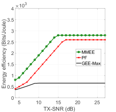
Figure 1: The performance of the weakest user with different beamforming designs.

Firstly, in Fig. 1 we present the achieved EE of the weakest user in the system with different beamforming designs, namely GEE-Max, PF, and MMEE designs. As can be seen in Fig. 1, the performance of the weakest user is significantly improved in terms of EE when considering the MMEE and PF-based designs compared to the conventional GEE-Max-based design. For example, at TX-SNR=20 dB, the weakest user experiences an EE of around $2800$ bits/Joule with the MMEE design, which is almost five times that of the EE that can be achieved with the GEE-Max-based design. Similarly, the PF-based design outperforms the GEE-Max-based design in terms of the performance for the weakest user. However, MMEE achieves the best EE for the weakest user compared to the other two designs. This is because MMEE maximizes the minimum achievable EE between all the users and attains the same EE for all users.

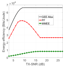
Figure 2: EE of the system (i.e., GEE) with different EE-based designs.

Next, we compare the achieved EE of the system (i.e., GEE) for different designs in Fig. 2. As expected, the GEE-Max design outperforms the other fairness-based designs in terms of the EE of the system, whereas the MMEE-based design shows the worst GEE performance between the three schemes presented in Fig. 2. However, the PF-based design attains a good balance between the EE at the system level and the achieved individual EE for each user. In other words, the PF-based design shows a better GEE compared to that of the MMEE-based design. The same design significantly improves EE of the weakest user compared to that of the GEE-Max-based design.

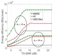
Figure 3: The weakest user’s performance with different designs at different weak users’ distances from the BS.

Finally, Fig. 3 illustrates the effect of weakest user distance (i.e., $d_{3}$) on its EE performance via different beamforming designs. As seen, the EE of the weakest user decreases as the distance from the BS increases.

V Conclusions

In this paper, we proposed two beamforming designs for a MISO NOMA system considering the EE fairness between users. The proposed designs are based upon the MMEE and PF. In particular, we formulated the designs as optimization problems, and applied the SCA technique to address the non-convexity nature of the original problems. Furthermore, simulation results showed that the MMEE-based design offers the best performance in terms of the weakest user EE when compared to the other designs. However, this improvement was attained at the cost of the GEE degradation of the system. Furthermore, the PF-based design shows a good balance between the GEE performance and the achieved EE of the weakest user.

References

- [1] Y. Saito, Y. Kishiyama, A. Benjebbour, T. Nakamura, A. Li, and K. Higuchi, “Non-orthogonal multiple access (NOMA) for cellular future radio access,” in Proc. IEEE VTC Spring, 2013, pp. 1–5.
- [2] S. Tomida and K. Higuchi, “Non-orthogonal access with SIC in cellular downlink for user fairness enhancement,” in Proc. Inter. Symp. on Intell. Signal Process. and Comm. Systems (ISPACS), 2011, pp. 1–6.
- [3] S. R. Islam, N. Avazov, O. A. Dobre, and K.-S. Kwak, “Power-domain non-orthogonal multiple access (NOMA) in 5G systems: potentials and challenges,” IEEE Commun. Surveys Tuts., 2017.
- [4] F. Alavi, K. Cumanan, Z. Ding, and A. G. Burr, “Beamforming techniques for non-orthogonal multiple access in 5G cellular networks,” IEEE Trans. Veh. Technol., vol. 67, no. 10, pp. 9474–9487, Oct. 2018.
- [5] Z. Chen, Z. Ding, P. Xu, and X. Dai, “Optimal precoding for a QoS optimization problem in two-user MISO-NOMA downlink,” IEEE Commun. Lett., vol. 20, no. 6, pp. 1263–1266, Jun. 2016.
- [6] Z. Ding, F. Adachi, and H. V. Poor, “The application of MIMO to non-orthogonal multiple access,” IEEE Trans. Wireless Commun., vol. 15, no. 1, pp. 537–552, Jan. 2016.
- [7] F. Alavi, K. Cumanan, Z. Ding, and A. G. Burr, “Robust beamforming techniques for non-orthogonal multiple access systems with bounded channel uncertainties,” IEEE Commun. Lett., vol. 21, no. 9, pp. 2033–2036, 2017.
- [8] R. Vannithamby and S. Talwar, Towards 5G applications: requirements and candidate technologies. John Wiley & Sons, 2017.
- [9] H. Alobiedollah, K. Cumanan, J. Thiyagalingam, A. G. Burr, Z. Ding, and O. A. Dobre, “Energy efficient beamforming design for MISO non-orthogonal multiple access systems,” Accepted on IEEE Trans. Commun., Feb. 2019.
- [10] A. Zappone and E. Jorswieck, “Energy efficiency in wireless networks via fractional programming theory,” Found. Trends Commun. Inf. Theory, vol. 11, no. 3-4, pp. 185–396, Jan. 2015.
- [11] H. Shi, R. V. Prasad, E. Onur, and I. Niemegeers, “Fairness in wireless networks: Issues, measures and challenges,” IEEE Commun. Surveys Tuts., vol. 16, no. 1, pp. 5–24, 2014.
- [12] D. Bertsimas, V. F. Farias, and N. Trichakis, “The price of fairness,” Operations Research, vol. 59, no. 1, pp. 17–31, 2011.
- [13] K. Cumanan, R. Krishna, Z. Xiong, and S. Lambotharan, “Sinr balancing technique and its comparison to semidefinite programming based qos provision for cognitive radios,” in Proc. VTC Spring. IEEE, 2009, pp. 1–5.
- [14] B. Radunović and J.-Y. L. Boudec, “A unified framework for max-min and min-max fairness with applications,” IEEE/ACM Trans. Netw. (TON), vol. 15, no. 5, pp. 1073–1083, Oct. 2007.
- [15] F. Kelly, “Charging and rate control for elastic traffic,” Trans. on Emerging Telecommunications Techn., vol. 8, no. 1, pp. 33–37, Feb. 1997.
- [16] M. F. Hanif, Z. Ding, T. Ratnarajah, and G. K. Karagiannidis, “A minorization-maximization method for optimizing sum rate in the downlink of non-orthogonal multiple access systems,” IEEE Trans. Signal Process., vol. 64, no. 1, pp. 76–88, Jan. 2016.
- [17] S. Vanka, S. Srinivasa, Z. Gong, P. Vizi, K. Stamatiou, and M. Haenggi, “Superposition coding strategies: Design and experimental evaluation,” IEEE Trans. Wireless Commun., vol. 11, no. 7, pp. 2628–2639, Jul. 2012.
- [18] P. Xu, K. Cumanan, and Z. Yang, “Optimal power allocation scheme for noma with adaptive rates and alpha-fairness,” in Proc. IEEE GLOBECOM, 2017, pp. 1–6.
- [19] M. Grant, S. Boyd, and Y. Ye, “CVX: Matlab software for disciplined convex programming,” [Online]. Available: http://www.stanford.edu/boyd/cvx.
- [20] O. Tervo, L.-N. Tran, and M. Juntti, “Optimal energy-efficient transmit beamforming for multi-user MISO downlink,” IEEE Trans. Signal Process., vol. 63, no. 20, pp. 5574–5588, Oct. 2015.
- [21] A. Beck, A. Ben-Tal, and L. Tetruashvili, “A sequential parametric convex approximation method with applications to nonconvex truss topology design problems,” J. Global Optimiz., vol. 47, no. 1, pp. 29–51, 2010.
- [22] Z.-Q. Luo and W. Yu, “An introduction to convex optimization for communications and signal processing,” IEEE J. Sel. Areas Commun., vol. 24, no. 8, pp. 1426–1438, Aug. 2006.
- [23] H. Alobiedollah, K. Cumanan, J. Thiyagalingam, A. G. Burr, Z. Ding, and O. A. Dobre, “Sum rate fairness trade-off-based resource allocation technique for MISO NOMA systems,” in Proc. IEEE WCNC’19.
- [24] K. Cumanan, R. Krishna, V. Sharma, and S. Lambotharan, “Robust interference control techniques for multiuser cognitive radios using worst-case performance optimization,” in Proc. Asilomar Conf. Signal, Syst. Comput. IEEE, 2008, pp. 378–382.