Numerical initial data deformation exploiting a gluing construction: I. Exterior asymptotic Schwarzschild

Abstract.

In this work a new numerical technique to prepare Cauchy data for the initial value problem (IVP) formulation of Einstein’s field equations is presented. Directly inspired by the exterior asymptotic gluing (EAG) result of Corvino [24] our (pseudo)-spectral scheme is demonstrated under the assumption of axisymmetry so as to fashion composite Hamiltonian constraint satisfying initial data featuring internal binary black holes (BBH) as glued to exterior Schwarzschild initial data in isotropic form. The generality of the method is illustrated in a comparison of the ADM mass of EAG initial data sets featuring internal BBHs as modelled by Brill-Lindquist and Misner data. In contrast to the recent work of Doulis and Rinne [28], and Pook-Kolb and Giulini [74] we do not make use of the York-Lichnerowicz conformal framework to reformulate the constraints.

1. Introduction

Gluing techniques provide for a powerful method of geometric analysis (GA) which may be exploited to combine multiple, distinct, solutions to a (system of) PDE of interest through their gradual deformation over some open set $\Omega$ so as to furnish a new, composite solution that approximately coincides with the original solutions away from $\Omega$ [16, 25, 17].

In this work we focus on the vacuum Einstein constraint equations $\mathcal{C}^{\mathrm{ADM}}[g,\,K]=0$ [22, 5, 72, 44, 80]. For concreteness, recall that the constraints split into the scalar Hamiltonian constraint $\mathcal{H}^{\mathrm{ADM}}[g,\,K]=0$ and the vectorial momentum constraint $\mathcal{M}{}_{j}^{\mathrm{ADM}}[g,\,K]=0$. In general, these are to be satisfied on a Riemannian manifold $\Sigma$ by a spatial metric $g_{ij}$, together with extrinsic curvature $K_{ij}$. From the perspective of the (numerical) evolution problem, a triplet $(\Sigma,\,g_{ij},\,K_{ij})$ constitutes an initial data set.

Consider a moment-in-time (MIT) symmetry (where $K_{ij}=0$), such that the constraints reduce to the single, scalar-flat condition $\mathcal{R}[g]=0$. In this setting, by exploiting a GA based technique of scalar curvature deformation, Corvino [24] has shown the following: let $g$ be an arbitrary asymptotically flat metric on $\mathbb{R}^{3}$, satisfying the Hamiltonian constraint $\mathcal{R}[g]=0$, with positive ADM-mass $m_{0}$. Then there exists another asymptotically flat metric $\hat{g}$ satisfying the constraint which agrees with $g$ on a compact set $K_{1}$ and is identical to a Schwarzschild solution (with, in general, a different ADM-mass and a shifted centre of mass) outside another compact set $K_{2}$ with $K_{1}\Subset K_{2}$. Thus, the new metric may be regarded as a composite metric obtained by gluing the original metric to the Schwarzschild metric in the transition region $\Omega:=K_{2}\backslash K_{1}$. The truly novel feature of this exterior asymptotic gluing (EAG) construction is that the new composite initial data set exactly coincides with its respective constituents outside the “transition region” $\Omega$ (which, as an example, may be imagined to be a spherical shell of finite thickness). This possibility of local gluing, where the region over which two initial data sets are spliced together is of compact support, is entirely due to the underdeterminedness of the constraint equations. The assumption of asymptotic flatness for the interior metric seems to have been made for technical reasons in order to guarantee that the non-linear operator in question is surjective. In the present work we stick with this assumption and glue only metrics which are asymptotically flat. It would be interesting, however, to see whether Corvino’s approach would also allow us to glue arbitrary scalar-flat metrics.

By relaxing the MIT condition and applying a similar gluing strategy it has been shown that the Corvino-Schoen technique may also be used to glue to exact Kerr exteriors [26]. Thus, quite general interior gravitational configurations may be glued to exterior Schwarzschild or Kerr regions forming a composite solution with precise asymptotics.

A striking variant of the above, where $\Omega$ is replaced by a conical region of infinite extent, is Carlotto-Schoen gluing [15] (see also [17]). In principle, effective screening is allowed for by manipulation of vacuum initial data alone. Furthermore, the Corvino-Schoen and Carlotto-Schoen gluings may be utilised so as to construct $N$-body initial data sets [18].

Related to the above is the method of connected sum or IMP gluing [53, 52, 54]. Here the conformal (Lichnerowicz-York) framework is adopted and consequently a determined elliptic system results. Given any two solutions of the constraints: $(\check{\Sigma}_{0},\,\check{g}_{ij},\,\check{K}_{ij})$ and $(\hat{\Sigma}_{0},\,\hat{g}_{ij},\,\hat{K}_{ij})$, say, a new solution may be produced by first removing small neighbourhoods $\check{N}$ and $\hat{N}$ about the points $\check{p}\in\check{\Sigma}_{0}$ and $\hat{p}\in\hat{\Sigma}_{0}$ respectively. Then, new data $(\Sigma_{0},\,g_{ij},\,K_{ij})$ is found by connecting $\partial\check{N}$ along an interpolating tube to $\partial\hat{N}$ with $\Sigma_{0}$ resulting in a connected sum manifold with the topology of $\check{\Sigma}_{0}\#\hat{\Sigma}_{0}$. By suitable interpolation of the pairs $(\check{g}_{ij},\,\check{K}_{ij})$ and $(\hat{g}_{ij},\,\hat{K}_{ij})$ a composite constraint satisfying solution $(\Sigma_{0},\,g_{ij},\,K_{ij})$ may be found.

Alternatively, identifying $\check{\Sigma}_{0}$ and $\hat{\Sigma}_{0}$ allows for a handle (wormhole) to be introduced to a given initial data set. On account of the determinedness this leads to a global deformation of the initial data set which is small away from the gluing site. By combining the results of [24, 19] it was shown in [20, 21] how the deformation may be localised. To date there do not appear to have been attempts made to prepare numerical initial data based on the IMP approach.

Aside from the ability to control asymptopia of initial data sets, engineering of exotic properties is interesting in its own right and, indeed, a robust scheme for fashioning numerical solutions could prove useful in endowing the associated space-time with a particular, desired phenomenology. For example, inspired by the result of [24], a potential path towards minimisation of so-called “spurious” gravitational radiation content was provided in [41]. We refer the reader there for further details.

While the above gluing results have intriguing properties, an unfortunate aspect is that the GA flavour of proof technique is quite technical in nature. It is not entirely clear how to proceed if direct numerical preparation of an initial data set based on such methods is desired. This is evidenced by the fact that there exists only a single attempt [41] based on formal perturbation theory to “embed” within the conformal framework a problem that seeks to mimic the setup of Corvino’s result [24].

Briefly, the idea in [41] was to work at an MIT symmetry, assume axisymmetry and fix internal Brill-Lindquist (BL) data. Then, over an annular $\Omega$ a conformally transformed Brill-Wave [12] ansatz on the form of the conformal factor $\psi$ is made. It was claimed that composite solutions exist to this problem when the exterior is a suitably chosen Schwarzschild initial data set. This approach requires a further, ad hoc treatment of the decay rates of $\psi$ as $\partial\Omega$ is approached. Following this programme, it appears that a numerical solution may be constructed [28] (see however, the modified, Newton-Krylov based approach of [74]).

An additional insight is offered in [28] as to how consistent selection of exterior data (or parameters on valid internal data) may be made by exploitation of an integrability condition. Such arguments are not required in the proof of [24]. It does not appear that numerical evolution has been performed based on the results of [28, 74]. Indeed, we are not aware of any numerical evolution of initial data sets which have been prepared based on gluing techniques.

More broadly, the technique of scalar curvature deformation may be of potential interest in studies involving geometric curvature flow. Such flows were introduced to general relativity in [37] and the idea built upon in [55] to rule out a class of counterexamples to the cosmic censorship hypothesis proposed by Penrose in [70] as encapsulated by an inequality relating black hole (ADM) mass and the area of its apparent horizon. The veracity of this inequality in a special case was first established rigorously in [51] by exploiting the inverse mean curvature flow for MIT data sets. The more general problem without this restriction remains open and numerical investigation utilising the weak formulation approach of [51] may help shed light on the matter. The related Ricci flow [47] has also been studied numerically [35, 78] where in [35] preliminary evidence for critical behaviour along the flow was presented. Another potentially novel scenario to consider may be whether scalar curvature deformation can be employed as a mechanism to control the appearance of such critical behaviour.

Our goal in this work is to provide some insight as to how the proof in [24] may be more directly adapted to a numerical technique itself without making use of the conformal programme for reformulation of the constraint equations as in [41, 28, 74]. In so doing, we shall numerically construct initial data as composite solutions with an MIT symmetry. To begin, we elaborate upon Corvino’s method at a formal level in §2. Scalar curvature deformation over $\Omega\Subset\Sigma$ and construction of a solution metric describing it, is effected iteratively, through solution of a sequence of linear sub-problems. The basic ingredient of this is described in §2.1. How the iteration is to proceed, together with an obstruction that occurs in the particular case of solving the constraints themselves and our proposed remedy is detailed in §2.2.

Having outlined the problem at the abstract level we next turn our attention to providing a robust description of geometric quantities required for the problem that is suitable for numerical work. To this end, a frame based approach is introduced in §3. In particular, $\Sigma$ is viewed as foliated by topological $2$-spheres. With a view towards efficient numerical implementation, the intrinsic geometry is described through the $\eth$-formalism, which is briefly recounted in §3.1. Details on how it may be adapted to treat topological $2$-spheres are provided in §3.2. For convenience, the relation between intrinsic and ambient quantities adapted to our discussion is touched upon in §3.3.

The success and versatility of pseudo-spectral methods [45] motivates our numerical approach in §4. In particular, function approximation of intrinsic quantities cast in the $\eth$-formalism is discussed in §4.1. Approximation of more general quantities over $\Sigma$ is described in §4.2. For the deformation problem at hand, we supplement the discussion with some complex analytic considerations that can assist in improving numerical solution quality in §4.3.

With particulars of the physical problem and numerical technique fixed we subsequently investigate prototype problems in §5. As an initial test, the case of scalar curvature deformation in the context of spherical symmetry is initially investigated in §5.1, and self-consistent convergence tests performed in §5.2. Following this, a relaxation to the class of axisymmetric problems is set up in §5.3 and explored in §5.4. In §5.5 all previously introduced material is brought together and we perform gluing of internal BBH data (for Brill-Lindquist and Misner initial data) to exterior Schwarzschild initial data. Numerical performance of the approach together with properties of the physical construction are investigated. Finally §6 concludes.

2. Corvino’s method

The argument for solving the Einstein constraints $\mathcal{C}^{\mathrm{ADM}}[g,\,K]=0$ presented in [24] by virtue of exterior asymptotic gluing (EAG) is quite technical in nature and consequently how one should proceed in order to fashion a numerical technique is somewhat opaque. Our goal here is to provide a sketch of the idea adapted to the aforementioned context (cf. the general discussions of [3, 17, 16, 25]). The physical setting is vacuum with vanishing cosmological constant at an MIT symmetry $(K_{ij}=0)$ and in what follows $\Sigma$ is to be understood as an initial Cauchy slice. Under these assumptions $\mathcal{C}^{\mathrm{ADM}}[g,\,K]=0$ reduces to the single, non-trivial, scalar-flat condition $\mathcal{R}[g]=0$ and $(\Sigma,\,g)$ is sought.

To explain EAG and fix the desired behaviour of $g$ recall that asymptotically flat (AF) data are characterised by the existence of a diffeomorphism between the “end” of $\Sigma$ and $\mathbb{R}^{3}$ with a ball $\mathbb{B}$ removed. Let $\delta_{\mathrm{Euc}}$ be the Euclidean metric. For AF $(\Sigma,\,g_{E})$, end coordinates $\{x^{i}\}_{i=1:3}$ may be introduced such that decay of $g_{E}$ (and derivatives thereof) to $\delta_{\mathrm{Euc}}$ is controlled by negative powers of $|x|$ (see [3, 17]).

The result of [24] concerns an equivalence class of Schwarzschild initial data where a representative in isotropic form is provided by:

$$g_{S}=\left(1+\frac{M_{\mathrm{ADM}}}{2|\mathbf{x}-\mathbf{C}|}\right)^{4}\delta_{\mathrm{Euc}},$$ (2.1)

and the $(1+3)$-parameter tuple $(\mathrm{M}_{\mathrm{ADM}},\,C^{i})$ describes the ADM mass and centre of mass. We identify $\Sigma$ with its image in $\mathbb{R}^{3}$. Let $\mathbb{B}_{\rho}\subset\Sigma$ be the ball of radius $\rho>0$. Introduce the compactly contained domain $\Sigma\Supset\Omega_{\rho}:=\mathbb{B}_{2\rho}\setminus\mathbb{B}_{\rho}$ the closure of which is a spherical shell of thickness $\rho$ and serves as a “transition region”. A selection of sufficiently large $\rho$ allows one to smoothly combine any AF $(\mathbb{B}_{\rho},\,{g}_{E})$ satisfying the scalar-flat condition ${\mathcal{R}}[g_{E}]=0$ with $(\Sigma\setminus\mathbb{B}_{2\rho},\,{g}_{S})$ over $\Omega_{\rho}$ via judicious selection of $g_{S}$. This latter is accomplished through tuning of the parameters $(\mathrm{M}_{\mathrm{ADM}},\,C^{i})$ and iterative correction of a smooth, interpolating “background metric” $\overline{g}_{\Omega_{\rho}}$. To understand the procedure, introduce the smooth cut-off function $\chi$ equal to $1$ on $\mathbb{B}_{\rho}$ and $0$ outside $\mathbb{B}_{2\rho}$, and on $\Omega_{\rho}$ set:

$$\overline{g}_{\Omega_{\rho}}:=\chi g_{E}+(1-\chi)g_{S}.$$ (2.2)

Clearly, ${\mathcal{R}}[\overline{g}_{\Omega_{\rho}}]=0$ on $\Sigma\setminus\Omega_{\rho}$ whereas on $\Omega_{\rho}$ we have ${\mathcal{R}}[\overline{g}_{\Omega_{\rho}}]=\delta$ where $\delta$ is a compactly supported function. Furthermore, we shall assume that ${\mathcal{R}}[\overline{g}_{\Omega_{\rho}}]$ is non-constant on $\Omega_{\rho}$ to avoid a technical issue outlined in §7.

To proceed further, the problem is now viewed as a local (i.e., compactly supported) deformation of the scalar curvature. Consider the change $\delta\rightarrow\check{\delta}:={\mathcal{R}}[\overline{g}_{\Omega_{\rho}}]+\tilde{\delta}$ for $\tilde{\delta}$ sufficiently small. The idea is to seek a suitable correction $h$ to the background metric such that ${\mathcal{R}}[\overline{g}_{\Omega_{\rho}}+h]=\check{\delta}$ is satisfied. The approach of [24] is to linearise about the background metric:

$${\mathcal{R}}[\overline{g}_{\Omega_{\rho}}+h]\simeq{\mathcal{R}}[\overline{g}_{\Omega_{\rho}}]+{L}_{\overline{g}_{\Omega_{\rho}}}[h],$$ (2.3)

where the linear problem ${L}_{\overline{g}_{\Omega_{\rho}}}[h]=\tilde{\delta}$ is investigated so as to characterise properties of the underdetermined elliptic operator $L_{\overline{g}_{\Omega_{\rho}}}$. Unfortunately, ${L}_{\overline{g}_{\Omega_{\rho}}}$ fails to be injective and the question of surjectivity of ${L}_{\overline{g}_{\Omega_{\rho}}}$ is addressed with a demonstration of injectivity of the formal adjoint ${L}^{*}_{\overline{g}_{\Omega_{\rho}}}$ which is overdetermined. This latter is then utilised, working within weighted function spaces yielding a so-called “basic estimate” over $\Omega_{\rho}$ where a certain growth (decay) rate of functions near $\partial\Omega_{\rho}$ is permitted. Thus, boundary behaviour of functions is implicitly controlled by a weight-function $\omega$ allowing for a variational based solution to the above linear problem. The control on properties of the linear solution turns out to be sufficiently strong to also allow for a Picard iteration scheme to obtain the solution $h$ to the nonlinear local deformation problem.

In principle, the problem of finding $h$ with ${\mathcal{R}}[\overline{g}_{\Omega_{\rho}}+h]=0$ may also be pursued in this way. However, an obstruction exists in that an approach to the scalar-flat condition, as for instance when ${\overline{g}}_{\Omega_{\rho}}\rightarrow{g}_{S}$, induces an approximate, non-trivial kernel $\mathscr{K}[{\overline{g}_{\Omega_{\rho}}}]:=\ker({L}_{\overline{g}_{\Omega_{\rho}}}^{*})$ of the formal linear adjoint. This may be ameliorated through judicious selection of $(M_{\mathrm{ADM}},C^{i})$ so as to work in a space transverse to $\ker({L}_{\delta_{\mathrm{Euc}}}^{*})$ when solving the previously described variational problem at the linearised level. Unfortunately, while [24] demonstrates that such a selection exists a method for a priori specification of the parameters is not provided and hence we instead adopt a direct, numerical linear-algebraic strategy.

We now proceed to provide further details of the variational approach to solving the linearised problem in §2.1 with sufficient detail for our numerical scheme. The nonlinear deformation shall be addressed in §2.2 together with our method for approaching the issue of non-trivial kernel.

2.1. Linear corrections via weak-formulation

For the sake of exposition we shall assume geometric quantities to be defined with respect to $\Omega:=\Omega_{\rho}$. Background quantities will be denoted by an over-bar. Furthermore, we shall assume that $\overline{\mathcal{R}}$ is non-constant. Suppose that a sufficiently small, smooth, local deformation (i.e. of compact support) of the scalar curvature is made $\mathcal{R}[\overline{g}]\rightarrow\mathcal{R}[g]:=\mathcal{R}[\overline{g}]+\tilde{\delta}$ and a metric correction $h$ satisfying $g=\overline{g}+h$ is sought. The problem may be investigated perturbatively by noting that formally $\overline{g}_{ij}\rightarrow g_{ij}=\overline{g}_{ij}+\varepsilon h_{ij}$ induces a corresponding linear-order correction to the scalar curvature $\mathcal{R}[g+\varepsilon h]=\mathcal{R}[\overline{g}]+\varepsilon L_{\overline{g}}[h]$ where standard methods yield [84]:

$$L_{\overline{g}}[h]=-h^{ij}\overline{\mathrm{Ric}}_{ij}-\overline{\nabla}^{2}\left[h^{k}{}_{k}\right]+\overline{\nabla}_{i}\overline{\nabla}_{j}h^{ij}.$$ (2.4)

Thus, solution of $L_{\overline{g}}[h]=\tilde{\delta}$ is required and hence properties of the linear operator $L_{\overline{g}}$ are investigated in [24]. While it turns out that $L_{\overline{g}}$ is underdetermined elliptic one may instead work with the formal $\mathrm{L}^{2}$ adjoint $\mathrm{L}{}^{*}_{\overline{g}}[\cdot]_{ij}$ as identified from the inner product $\langle\mathrm{L}{}_{\overline{g}}[h],\,f\rangle_{\mathrm{L}^{2}(\Omega)}=\langle h,\,\mathrm{L}{}^{*}_{\overline{g}}[f]\rangle_{\mathrm{L}^{2}(\Omega)}$:

$$\left(L_{\overline{g}}^{*}[f]\right)_{ij}=-\overline{\mathrm{Ric}}_{ij}f-\overline{g}_{ij}\overline{\nabla}^{2}\left[f\right]+\overline{\nabla}_{(i}\overline{\nabla}_{j)}[f],$$ (2.5)

which is injective [24] (see also §7). Introduce the weighted, Sobolev space functional $\mathcal{V}:H^{2}_{\omega}(\Omega)\rightarrow\mathbb{R}$ defined by:

$$\mathcal{V}[u]=\int_{\Omega}\left(\frac{1}{2}\|L_{\overline{g}}^{*}u\|^{2}-\tilde{\delta}u\right)\omega\,\mathrm{d}{\mu_{\overline{g}}},$$ (2.6)

where $\tilde{\delta}\in\mathrm{L}^{2}_{\omega}(\Omega)$, $\omega$ is a weight function (to be defined) and $\mathrm{d}{\mu}_{\overline{g}}$ is the integration measure induced by $\overline{g}$. To find the unique $u$ satisfying (2.6), we introduce the test-function $\eta\in C^{\infty}_{c}(\Omega)$ and consider the variation:

$$0=\left.\frac{d}{dt}\left[\mathcal{V}[u+t\eta]\right]\right|_{t=0}\quad\Longrightarrow\quad\int_{\Omega}\left[L_{\overline{g}}^{*}\eta\right]^{ij}\left[L_{\overline{g}}^{*}u\right]_{ij}\omega\,\mathrm{d}{\mu_{\overline{g}}}=\int_{\Omega}\eta\tilde{\delta}\omega\,\mathrm{d}{\mu_{\overline{g}}},$$ (2.7)

where the compact support of $\eta$ (or alternatively a presumed decay rate for $\omega$ towards $\partial\Omega$) enables us to drop all boundary terms. Equation (2.7) is the so-called weak-formulation [30, 67, 38] of the following strong-form problem [24]):

$$L_{\overline{g}}\left[\omega L_{\overline{g}}^{*}\left[u\right]\right]=\tilde{\delta}\omega=\delta,\quad\left(\delta\in C^{k,\,\alpha}_{\omega^{-1}}(\Omega)\right),$$ (2.8)

where $C^{k,\,\alpha}_{\omega^{-1}}(\Omega)$ is a weighted Hölder space [24]. In light of this equivalence and later use of Eq.(2.7) to iteratively construct $h$ we shall refer to $u$ as a “potential function”. In order to ensure future enforcement of $u\in H{}^{2}_{\omega}(\Omega)$ in Eq.(2.7) at the numerical level — indeed allowing for controlled growth of $u$ towards $\partial\Omega$ — an explicit rewriting exploiting the decay properties of the weight term $\omega$ can be made and viewed as a solution ansatz.

Suppose $x$ is a boundary defining function in a neighbourhood of $\partial\Omega$, i.e., $x\geq 0$ with $x=0$ and $\mathrm{d}x\neq 0$ on $\partial\Omega$. Suppose $\omega\sim x^{2N}$ for $N$ sufficiently large. The condition $\partial{}^{k}_{x}[u]\in L^{2}_{\omega}(\Omega)$ where $k\in\{0,\,1,\,2\}$ leads to:

$$u =\mathcal{N}\tilde{u}\omega^{\beta}, \beta =-\frac{1}{2};$$ (2.9)

where $\mathcal{N}$ is a function with quadratic decay in $x$ towards $\partial\Omega$ and $\tilde{u}$ shall be assumed to be bounded and smooth. We shall defer explicit specification of $\omega$ to §5.

2.2. Nonlinear local $\mathcal{R}$ deformation and gluing

The problem we would now like to solve is: On $\Sigma$ fix a choice of $\overline{g}$ and hence $\overline{\mathcal{R}}$ and $L{}_{\overline{g}}$ together with $\delta$ of compact support on $\Omega$. Assume that $\overline{\mathcal{R}}$ is non-constant. Find a symmetric $2$-tensor $h\in\mathcal{S}_{2}(\Sigma)$ with compact support on $\Omega$ such that $\mathcal{R}[\overline{g}+h]=\mathcal{R}[\overline{g}]+\delta$.

Theorem $1$ of [24] allows us to proceed as follows: Set ${}^{(0)}\delta:=\mathcal{R}[g]-\mathcal{R}[\overline{g}]$, solve Eq.(2.7) for ${}^{(0)}u$, and hence construct ${}^{(0)}h_{ij}=\omega L{}_{\overline{g}}^{*}[{}^{(0)}u]_{ij}$. This yields ${}^{(1)}g_{ij}=\overline{g}_{ij}+{}^{(0)}h_{ij}$ with ${}^{(0)}h_{ij}$ small in an appropriate Hölder space. Now, it would be natural to apply Newton’s method and linearise about the new metric ${}^{(1)}g_{ij}$. However, it turns out [24] that this would apparently result in a loss of differentiability. Instead the proof technique leverages Picard iteration with the linearisation fixed at the background $\overline{g}_{ij}$ and the approximate solution is iteratively improved via:

$${}^{(k)}\delta=\mathcal{R}[g_{ij}]-\mathcal{R}\left[\overline{g}_{ij}+\omega\sum^{k-1}_{m=0}{}^{(m)}\tilde{h}_{ij}\right],$$ (2.10)

where ${}^{(m)}\tilde{h}_{ij}:=L_{\overline{g}}^{*}\left[{}^{(m)}u\right]$ and the solution (metric) is given by $g_{ij}=\overline{g}_{ij}+\lim_{N\rightarrow\infty}\omega\sum_{m=0}^{N}{}^{(m)}\tilde{h}_{ij}$.

An issue remains when $\overline{\mathcal{R}}$ is constant and correspondingly a non-trivial kernel $\mathscr{K}[\overline{g}]:=\ker(L_{\overline{g}}^{*})$ exists. This must be addressed if exterior asymptotic gluing (EAG) to a time-symmetric slice of Schwarzschild $g_{S}$ is to be achieved and a solution to the constraints found. Consider $\overline{g}_{\Omega_{\rho}}$ of Eq.(2.2). The dimension of $\mathscr{K}[\overline{g}_{\Omega_{\rho}}]$ is related to the underlying (approximate) symmetries of $\overline{g}_{\Omega_{\rho}}$ and due to the assumption of $\overline{g}_{\Omega_{\rho}}$ being asymptotically Euclidean must approach that of $\mathscr{K}[\delta_{\mathrm{Euc}}]$ in the asymptotic regime (described below) [16, 25]. It is also known that in linearisation of the full vacuum constraints (no longer at an MIT) a further contribution to the kernel of the corresponding formal linear adjoint arises, which is comprised of the generators of translation and rotation of $\mathbb{R}^{3}$ [16, 25]. Collectively, elements of the non-trivial kernel in this latter case are called Killing initial data (KID) due to the one-to-one correspondence with Killing vectors in the vacuum space-time obtained by evolving the initial data set [66].

Thus for EAG on Schwarzschild we clearly encounter an obstruction as $\rho$ is increased due to the fall-off properties of $\overline{g}_{\Omega_{\rho}}$ and approach to the non-trivial $\mathscr{K}[g_{S}]$. As a preliminary, notice that we can identify $\mathscr{K}_{0}:=\mathscr{K}[\delta_{\mathrm{Euc}}]=\mathrm{span}(1,\,x^{1},\,x^{2},\,x^{3})$. This can be seen by observing Eq.(2.5) implies:

$$L_{\delta_{\mathrm{Euc}}}^{*}[f]{}^{i}{}_{j}=-\delta{}^{i}{}_{j}\partial^{k}[\partial_{k}[f]]+\partial{}^{i}\partial{}_{j}[f],$$ (2.11)

and hence $L_{\delta_{\mathrm{Euc}}}^{*}[\cdot]_{ij}$ annihilates affine functions of the form $f=a+b_{k}x^{k}$ where $a\in\mathbb{R}$ and $b_{k}\in\mathbb{R}^{3}$. That these are the only possible functions then follows from considering the finite-dimensional space of initial data for Eq.(7.8).

Returning to EAG on Schwarzschild, note that we are only approximately approaching a non-trivial kernel. To account for this [24] proceeds by introducing an approximating kernel $\mathscr{K}_{*}:=\zeta\mathscr{K}_{0}$ where $\zeta$ is a smooth, spherically symmetric bump function of compact support on $\Omega_{\rho}$. The idea is then to solve a projected nonlinear local deformation problem based on $\overline{g}_{\Omega_{\rho}}$ as above but working with functions in the $\mathrm{L}^{2}(\Omega_{\rho})$ orthogonal complement of $\mathscr{K}_{*}$. When carried out at sufficiently large $\rho$ this yields a glued solution $g$ with $\mathcal{R}[g]\in\mathscr{K}_{*}$ and a choice of $(M_{\mathrm{ADM}},\,C^{i})$ is shown to exist (though it is not demonstrated how to select these parameters a priori) such that a $g$ with $\mathcal{R}[g]=0$ may be found.

For our numerical approach a slightly different strategy shall be pursued. An alternative way to construct an appropriately projected problem that treats non-trivial $\mathscr{K}_{0}$ indirectly is provided by linear algebraic techniques. The idea here is to consider evaluation of the weak-formulation statement of Eq.(2.7) with a suitably chosen dense, approximating collection of test space and solution (trial) space functions. A singular value decomposition (SVD) of the ensuing linear system may then be inspected and any (approximate) kernel directly removed [79].

During numerical calculations involving EAG on Schwarzschild (to be performed in §5.5) symmetry conditions shall be imposed. A precise identification of the dimension of the non-trivial kernel in this context may be motivated as follows: Consider the affine functions $f$ as annihilated by $L{}^{*}_{\delta_{\mathrm{Euc}}}[\cdot]_{ij}$. According to [3] the parameters $a$ and $b_{k}$ entering $f$ as above primarily affect how $M_{\mathrm{ADM}}$ and centre of mass $C^{i}$ should be chosen in the composite (numerical) solution. Thus in a context with a high degree of symmetry the effective dimension of the kernel may be reduced.

3. Frame-formalism treatment of $\Sigma$-geometry

With the physical problem and geometric preliminaries outlined in §2 we now turn our attention to concretising the formulation for numerical work. Given a $\Sigma$ with underlying symmetries a chart selection exploiting this property allows for a description of geometric quantities that can lead to more efficient numerical schemes (see §4). In order to accomplish this in a robust fashion, such that issues of regularity do not arise from the choice of coordinatisation we adopt a frame based approach that leverages the so-called $\eth$-formalism. It shall be assumed that $\Sigma$ is endowed with metric $g_{ij}$ and that $(\Sigma,\,g_{ij})$ may be smoothly foliated by a one-parameter family of non-intersecting topological $2$-spheres $\mathbb{S}{}^{2}_{\rho}$ which are to be viewed as the level surfaces of a smooth function $\rho:\Sigma\rightarrow\mathbb{R}$. Denote the Levi-Civita connection associated with $g_{ij}$ by ${\nabla}$.

Following the standard prescription of ADM decomposition adapted to a spatial manifold, the normalised 1-form $n_{i}=N{\nabla}_{i}[\rho]$ provides a normal to $\mathbb{S}{}^{2}_{\rho}$. Recall that the ambient metric induces the metric $\gamma_{ij}$ on the submanifolds $\mathbb{S}{}^{2}_{\rho}$ via $g_{ij}=\gamma_{ij}+n_{i}n_{j}$ and gives rise to the projector $\mathcal{P}{}^{i}{}_{j}:=\gamma{}^{i}{}_{j}-n^{i}n_{j}$. Supplementation with $\mathcal{N}{}^{i}{}_{j}:=n^{i}n_{j}$ allows for decomposition of type $(q,\,r)$ tensor fields, collectively denoted $\mathcal{T}{}^{q}_{r}(\Sigma)$, into intrinsic and normal parts. Introduce a smooth vector field $\rho^{i}\in\mathfrak{X}(\Sigma)$ satisfying $\rho^{i}{\nabla}{}_{i}[\rho]=1$. Then $\rho^{i}=Nn^{i}+N^{i}$ where $N^{i}=\mathcal{P}{}^{i}{}_{j}\rho^{j}$ and consequently the ambient metric may be decomposed via:

$$g_{ij}=(1-N^{-2}N_{K}N^{K})n_{i}n_{j}+2N^{-1}n{}_{(i}N_{j)}+\delta{}^{I}_{i}\delta{}^{J}_{j}\gamma_{IJ},$$ (3.1)

where capital Latin indices take values in $\{2,\,3\}$ and here $\delta$ is the Kronecker delta.

3.1. Intrinsic $2$-geometry and spin-weight

In order to further adapt the intrinsic $\mathbb{S}{}^{2}_{\rho}$ part of the geometry we take the view of [8, 7, 29]. Without going into too much detail we mention that the $\eth$-formalism is based on the fundamental relationships between the unit 2-sphere $\mathbb{S}^{2}$, its frame bundle and the group $\mathrm{SO}(3)$. In what follows we regard the 2-sphere as the unit-sphere equipped with the usual Euclidean metric. The bundle of frames over $\mathbb{S}^{2}$ is diffeomorphic to the rotation group since every rotation matrix consists of three orthonormal vectors which form an oriented basis of $\mathbb{R}^{3}$. Interpreting the first vector as a point $\mathbf{e}$ on $\mathbb{S}^{2}$, the other two vectors yield an orthonormal basis in the tangent space $T_{\mathbf{e}}\mathbb{S}^{2}$. Keeping $\mathbf{e}$ fixed we see that all frames at $\mathbf{e}$ are related by a 2-dimensional rotation, i.e., an element of $\mathrm{SO}(2)$. It is easily seen that this correspondence between frames on the 2-sphere and a rotation matrix is bijective and that it allows us to regard the $2$-sphere as the factor space $\mathrm{SO}(3)/{\mathrm{SO}(2)}$. The projection map $\pi:\mathrm{SO}(3)\rightarrow\mathbb{S}^{2}$ is called the Hopf map.

Every tensor field defined at a point $\mathbf{e}\in\mathbb{S}^{2}$ can be decomposed into components with respect to a basis in $T_{\mathbf{e}}\mathbb{S}^{2}$ and we may regard these components as functions defined at a particular point on $\mathrm{SO}(3)$. Since they are components of a tensor field they change in a very characteristic way when we change the basis in $T_{\mathbf{e}}\mathbb{S}^{2}$. In this way we can describe every tensor field on the sphere by a set of functions with special behaviour under change of basis. By regarding this set as a whole we have eliminated the need for referring to a particular choice of basis on the 2-sphere. This is the main advantage in this formalism since it is well known that there are no globally well defined frames on $\mathbb{S}^{2}$ — a fact, which creates many problems for numerical simulations involving the 2-sphere.

Next, we introduce appropriate Euler angles for rotations and polar coordinates on the 2-sphere so that we can express these well defined global relationships in local coordinates. The Hopf map can be expressed in these coordinates as $\pi:(\theta,\,\psi,\,\phi)\mapsto(\vartheta,\,\varphi)=(\theta,\,\phi)$.

Consider the open subset $U\subset\mathbb{S}^{2}$ away from the poles ($\vartheta=0,\,\pi$) such that the Hopf map with respect to the given coordinates is well-defined. A smooth (real) orthonormal frame $\hat{\mathbf{e}}_{(I)}$ on $U$ may be introduced where the parentheses indicate distinct frame fields. Define the complex field $\mathbf{m}:=\left(\hat{\mathbf{e}}_{(2)}+i\hat{\mathbf{e}}_{(3)}\right)/\mathchoice{{\hbox{$\displaystyle\sqrt{2\,}$}\lower 0.4pt\hbox{\vrule height=6.44444pt,depth=-5.15558pt}}}{{\hbox{$\textstyle\sqrt{2\,}$}\lower 0.4pt\hbox{\vrule height=6.44444pt,depth=-5.15558pt}}}{{\hbox{$\scriptstyle\sqrt{2\,}$}\lower 0.4pt\hbox{\vrule height=4.51111pt,depth=-3.6089pt}}}{{\hbox{$\scriptscriptstyle\sqrt{2\,}$}\lower 0.4pt\hbox{\vrule height=3.22221pt,depth=-2.57779pt}}}$. In terms of this complex linear combination we can express the action of $\mathrm{SO}(2)$ as multiplication with a phase $\mathbf{m}\mapsto\mathbf{m}^{\prime}=e^{i\psi}\mathbf{m}$ inducing rotation of the complex frame $(\mathbf{m},\,\overline{\mathbf{m}})$ together with its dual coframe ($\boldsymbol{\omega},\,\overline{\boldsymbol{\omega}})$ which leads to the notion of spin-weight [8]. Given a smooth tensor field $T\in\mathcal{T}{}^{q}_{r}(U)$ its (equivalent) spin-weighted representation is provided by:

$${}_{s}T:=T(\underbrace{\boldsymbol{\omega},\,\cdots\boldsymbol{\omega}}_{\mbox{\small$q_{1}$ times}};\,\underbrace{\overline{\boldsymbol{\omega}},\,\cdots,\,\overline{\boldsymbol{\omega}}}_{\mbox{\small$q_{2}$ times}};\,\underbrace{\mathbf{m},\,\cdots\mathbf{m}}_{\mbox{\small$r_{1}$ times}};\,\underbrace{\overline{\mathbf{m}},\,\cdots,\,\overline{\mathbf{m}}}_{\mbox{\small$r_{2}$ times}}),$$ (3.2)

where $s=r_{1}-r_{2}-q_{1}+q_{2}$ is the spin-weight.

The unit-sphere metric $\overset{\circ}{\gamma}$ on $\mathbb{S}^{2}$ when expressed in these coordinates acquires the form:

$$\overset{\circ}{\gamma} =\overset{\circ}{\gamma}_{IJ}\mathrm{d}{x}^{I}\otimes\mathrm{d}{x}^{J}=\mathrm{d}{\vartheta}\otimes\mathrm{d}{\vartheta}+\sin^{2}\vartheta\,\mathrm{d}{\varphi}\otimes\mathrm{d}{\varphi},$$ (3.3)

where the choice of coordinatisation entails that orthonormal frame vectors may be selected as $\hat{\mathbf{e}}_{(2)}=\partial_{\vartheta}$ and $\hat{\mathbf{e}}_{(3)}=\csc\vartheta\,\partial_{\varphi}$. The associated complex reference (co)frame becomes:

$$m^{I}=\frac{1}{\mathchoice{{\hbox{$\displaystyle\sqrt{2\,}$}\lower 0.4pt\hbox{\vrule height=6.44444pt,depth=-5.15558pt}}}{{\hbox{$\textstyle\sqrt{2\,}$}\lower 0.4pt\hbox{\vrule height=6.44444pt,depth=-5.15558pt}}}{{\hbox{$\scriptstyle\sqrt{2\,}$}\lower 0.4pt\hbox{\vrule height=4.51111pt,depth=-3.6089pt}}}{{\hbox{$\scriptscriptstyle\sqrt{2\,}$}\lower 0.4pt\hbox{\vrule height=3.22221pt,depth=-2.57779pt}}}}\left(\partial_{\vartheta}^{I}-i\csc\vartheta\,\partial_{\varphi}^{I}\right)\Longrightarrow\omega_{I}=\frac{1}{\mathchoice{{\hbox{$\displaystyle\sqrt{2\,}$}\lower 0.4pt\hbox{\vrule height=6.44444pt,depth=-5.15558pt}}}{{\hbox{$\textstyle\sqrt{2\,}$}\lower 0.4pt\hbox{\vrule height=6.44444pt,depth=-5.15558pt}}}{{\hbox{$\scriptstyle\sqrt{2\,}$}\lower 0.4pt\hbox{\vrule height=4.51111pt,depth=-3.6089pt}}}{{\hbox{$\scriptscriptstyle\sqrt{2\,}$}\lower 0.4pt\hbox{\vrule height=3.22221pt,depth=-2.57779pt}}}}\left(\mathrm{d}{\vartheta}_{I}+i\sin\vartheta\,\mathrm{d}{\varphi}_{I}\right),$$ (3.4)

subject to the complex orthonormality conditions:

$$m^{I}\overline{\omega}_{I}= 0, m^{I}\omega_{I}= 1; m^{I}m^{J}\overset{\circ}{\gamma}{}_{IJ}= 0, \omega_{I}\omega_{J}\overset{\circ}{\gamma}{}^{IJ}= 0; m^{I}\overline{m}^{J}\overset{\circ}{\gamma}{}_{IJ}= 1, \omega_{I}\overline{\omega}_{J}\overset{\circ}{\gamma}{}^{IJ}= 1.$$ (3.5)

On account of Eqs. 3.3, 3.4 and 3.5 we thus have:

$$\overset{\circ}{\gamma}{}_{IJ}= 2\omega_{(I}\overline{\omega}_{J)}, \overset{\circ}{\gamma}{}^{IJ}= 2m{}^{(I}\overline{m}{}^{J)}, \overset{\circ}{\gamma}{}^{I}{}_{J}= \overline{m}{}^{I}\overline{\omega}{}_{J}+\omega{}_{J}m{}^{I}=\delta{}^{I}_{J}.$$ (3.6)

Denote the Levi-Civita connection associated with $\overset{\circ}{\gamma}$ by $\overset{\circ}{\mathfrak{D}}$. We will now use this to define derivative operators which are adapted to the notion of spin-weight, mapping spin-weighted quantities to spin-weighted quantities. Suppose ${}_{s}f$ is a spin-weighted quantity in the sense of Eq.(3.2). We define the $\eth$ operators as components of the corresponding tensor field in the direction of $\mathbf{m}$ and $\overline{\mathbf{m}}$ as follows:

$$\mathbf{m}\left[{}_{s}f\right]= m^{I}\overset{\circ}{\mathfrak{D}}_{I}\left[{}_{s}f\right]=\frac{1}{\mathchoice{{\hbox{$\displaystyle\sqrt{2\,}$}\lower 0.4pt\hbox{\vrule height=6.44444pt,depth=-5.15558pt}}}{{\hbox{$\textstyle\sqrt{2\,}$}\lower 0.4pt\hbox{\vrule height=6.44444pt,depth=-5.15558pt}}}{{\hbox{$\scriptstyle\sqrt{2\,}$}\lower 0.4pt\hbox{\vrule height=4.51111pt,depth=-3.6089pt}}}{{\hbox{$\scriptscriptstyle\sqrt{2\,}$}\lower 0.4pt\hbox{\vrule height=3.22221pt,depth=-2.57779pt}}}}\eth\left[{}_{s}f\right]+{}_{s}fs\overset{\circ}{\Gamma}, \overline{\mathbf{m}}\left[{}_{s}f\right]= \overline{m}^{I}\overset{\circ}{\mathfrak{D}}_{I}\left[{}_{s}f\right]=\frac{1}{\mathchoice{{\hbox{$\displaystyle\sqrt{2\,}$}\lower 0.4pt\hbox{\vrule height=6.44444pt,depth=-5.15558pt}}}{{\hbox{$\textstyle\sqrt{2\,}$}\lower 0.4pt\hbox{\vrule height=6.44444pt,depth=-5.15558pt}}}{{\hbox{$\scriptstyle\sqrt{2\,}$}\lower 0.4pt\hbox{\vrule height=4.51111pt,depth=-3.6089pt}}}{{\hbox{$\scriptscriptstyle\sqrt{2\,}$}\lower 0.4pt\hbox{\vrule height=3.22221pt,depth=-2.57779pt}}}}\overline{\eth}\left[{}_{s}f\right]-{}_{s}fs\overset{\circ}{\Gamma};$$ (3.7)

where $\overset{\circ}{\Gamma}=m^{I}\overline{m}^{J}\overset{\circ}{\mathfrak{D}}_{J}\left[\omega_{I}\right]$ and for the choice of Eqs. 3.3 and 3.4 we have $\overset{\circ}{\Gamma}=\cot\vartheta/\mathchoice{{\hbox{$\displaystyle\sqrt{2\,}$}\lower 0.4pt\hbox{\vrule height=6.44444pt,depth=-5.15558pt}}}{{\hbox{$\textstyle\sqrt{2\,}$}\lower 0.4pt\hbox{\vrule height=6.44444pt,depth=-5.15558pt}}}{{\hbox{$\scriptstyle\sqrt{2\,}$}\lower 0.4pt\hbox{\vrule height=4.51111pt,depth=-3.6089pt}}}{{\hbox{$\scriptscriptstyle\sqrt{2\,}$}\lower 0.4pt\hbox{\vrule height=3.22221pt,depth=-2.57779pt}}}$ together with:

$$\eth\left[{}_{s}f(\vartheta,\varphi)\right]= (\sin\vartheta)^{s}\left(\partial_{\vartheta}-i\csc\vartheta\,\partial_{\varphi}\right)\left[(\sin\vartheta)^{-s}{}_{s}f(\vartheta,\varphi)\right],$$ (3.8)

$$\overline{\eth}\left[{}_{s}f(\vartheta,\varphi)\right]= (\sin\vartheta)^{-s}\left(\partial_{\vartheta}+i\csc\vartheta\,\partial_{\varphi}\right)\left[(\sin\vartheta)^{s}{}_{s}f(\vartheta,\varphi)\right].$$

Explicit translation formulae for covariant derivatives may be arrived at by virtue of Eq.(3.7) (see appendix of [76], but note conventions differ):

$$\mathchoice{{\hbox{$\displaystyle\sqrt{2\,}$}\lower 0.4pt\hbox{\vrule height=6.44444pt,depth=-5.15558pt}}}{{\hbox{$\textstyle\sqrt{2\,}$}\lower 0.4pt\hbox{\vrule height=6.44444pt,depth=-5.15558pt}}}{{\hbox{$\scriptstyle\sqrt{2\,}$}\lower 0.4pt\hbox{\vrule height=4.51111pt,depth=-3.6089pt}}}{{\hbox{$\scriptscriptstyle\sqrt{2\,}$}\lower 0.4pt\hbox{\vrule height=3.22221pt,depth=-2.57779pt}}}m^{J}m^{I_{1}}\cdots m^{I_{n}}\overset{\circ}{\mathfrak{D}}_{J}\left[W_{(I_{1}\cdots I_{n})}\right]= \eth\left[{}_{n}W\right], \mathchoice{{\hbox{$\displaystyle\sqrt{2\,}$}\lower 0.4pt\hbox{\vrule height=6.44444pt,depth=-5.15558pt}}}{{\hbox{$\textstyle\sqrt{2\,}$}\lower 0.4pt\hbox{\vrule height=6.44444pt,depth=-5.15558pt}}}{{\hbox{$\scriptstyle\sqrt{2\,}$}\lower 0.4pt\hbox{\vrule height=4.51111pt,depth=-3.6089pt}}}{{\hbox{$\scriptscriptstyle\sqrt{2\,}$}\lower 0.4pt\hbox{\vrule height=3.22221pt,depth=-2.57779pt}}}\overline{m}^{J}m^{I_{1}}\cdots m^{I_{n}}\overset{\circ}{\mathfrak{D}}_{J}\left[W_{(I_{1}\cdots I_{n})}\right]=\overline{\eth}\left[{}_{n}W\right].$$ (3.9)

Finally, we note that if the tensor field $W$ is real then under complex conjugation ${}_{+s}W^{*}={}_{-s}W$ and furthermore the operator actions $\eth\leftrightarrow\overline{\eth}$ are interchanged.

3.2. Topological $2$-spheres

In order to relax our treatment to more general geometries the assumption of §3.1 shall be modified and instead we shall consider working with a manifold $\mathbb{S}^{2}_{\rho}$ which is diffeomorphic to $\mathbb{S}^{2}$ but is equipped with a different metric. The approach we follow is based on [43, 76] and hence we shall only briefly summarise the idea here.

Consider the manifold $(\mathbb{S}{}^{2}_{\rho},\,\gamma{}_{IJ})$ endowed with metric:

$$\gamma{}_{IJ}={}_{-2}\gamma\overline{\omega}_{I}\overline{\omega}_{J}+2\,{}_{0}\gamma\omega_{(I}\overline{\omega}_{J)}+{}_{+2}\gamma\omega_{I}\omega_{J},$$ (3.10)

where the coframe is that of Eq.(3.4) and the expression follows from consideration of the irreducible decomposition of a type $(0,\,2)$ tensor field [43, 71]. The $\overset{\circ}{\gamma}$ of Eq.(3.3) is now demoted to the status of an auxiliary field. Thus, to be explicit, while the conditions of Eq.(3.5) continue to hold, indicial manipulations of tensorial quantities are now to be performed with $\gamma{}_{IJ}$. The inverse metric is given by:

$$\gamma^{IJ}={}_{0}\tilde{\gamma}\left(-{}_{-2}\gamma m^{I}m^{J}+2{}_{0}\gamma m^{(I}\overline{m}^{J)}-{}_{+2}\gamma\overline{m}^{I}\overline{m}^{J}\right),$$ (3.11)

where [43]:

$${}_{0}\tilde{\gamma}=\left({}_{0}\gamma^{2}-{}_{-2}\gamma{}_{+2}\gamma\right)^{-1}=\det(\overset{\circ}{\gamma}_{IJ})/\det\left(\gamma_{IJ}\right).$$ (3.12)

Note that:

$$\overline{\omega}^{I}=\gamma^{IJ}\omega_{J}= {}_{0}\tilde{\gamma}\left(-{}_{-2}\gamma m^{I}+{}_{0}\gamma\overline{m}^{I}\right), \omega^{I}=\gamma^{IJ}\overline{\omega}_{J}= {}_{0}\tilde{\gamma}\left({}_{0}\gamma m^{I}-{}_{+2}\gamma\overline{m}^{I}\right).$$ (3.13)

If coordinate components $(\vartheta,\,\varphi)$ are specified as:

$$\gamma_{IJ}=\begin{bmatrix}\Gamma_{1}&\Gamma_{2}\\ \Gamma_{2}&\Gamma_{3}\sin^{2}\vartheta\end{bmatrix},$$ (3.14)

then comparison with Eq.(3.4) and Eq.(3.10) yields:

$${}_{-2}\gamma= \frac{1}{2}(\Gamma_{1}-\Gamma_{3}+2i\Gamma_{2}\csc\vartheta), {}_{0}\gamma= \frac{1}{2}(\Gamma_{1}+\Gamma_{3}), {}_{+2}\gamma= \frac{1}{2}(\Gamma_{1}-\Gamma_{3}-2i\Gamma_{2}\csc\vartheta);$$ (3.15)

and $\Gamma_{i}\in\mathbb{R}$ implies ${}_{-2}\gamma={}_{+2}\gamma^{*}$. In order to complete the ingredients for a manifestly regular treatment of quantities in $\mathcal{T}{}^{q}_{r}(\mathbb{S}^{2}_{\rho})$ we require description of the covariant derivative operator in this new setting. Denote the Levi-Civita connection associated with $(\mathbb{S}{}^{2}_{\rho},\,\gamma_{IJ})$ by ${\mathfrak{D}}$. Then ${\mathfrak{D}}$ and $\overset{\circ}{\mathfrak{D}}$ may be uniquely related by introduction of a $(1,\,2)$ tensor field $C{}^{K}{}_{IJ}$ [84]:

$$C^{K}{}_{IJ}=C^{K}{}_{(IJ)}=\frac{1}{2}\gamma^{KL}\left(\overset{\circ}{\mathfrak{D}}_{I}[\gamma_{LJ}]+\overset{\circ}{\mathfrak{D}}_{J}[\gamma_{IL}]-\overset{\circ}{\mathfrak{D}}_{L}[\gamma_{IJ}]\right).$$ (3.16)

The tensor field $C^{K}{}_{IJ}$ arises as the difference between Christoffel symbols associated with each connection and consequently in evaluating the action of ${\mathfrak{D}}$ on a given field the pattern of additional terms matches that of the usually required $\Gamma{}^{K}{}_{IJ}$. For example, let $V\in\mathcal{T}{}^{0}_{1}(\mathbb{S}^{2}_{\rho})$ and $T\in\mathcal{T}{}^{0}_{2}(\mathbb{S}^{2}_{\rho})$ then:

$${\mathfrak{D}}_{I}[V_{J}]= \overset{\circ}{\mathfrak{D}}_{I}[V_{J}]-C^{K}{}_{IJ}V_{K},$$ (3.17)

$${\mathfrak{D}}_{I}[T_{JK}]= \overset{\circ}{\mathfrak{D}}_{I}[T_{JK}]-C^{L}{}_{IJ}T_{LK}-C^{L}{}_{IK}T_{JL}.$$

Furthermore, $C{}^{K}{}_{IJ}=\gamma{}^{KL}C{}_{LIJ}$ may itself be described in terms of spin-weighted components of the metric $\gamma$ and $\eth$ derivatives thereof via projection exploiting Eq.(3.2) and Eq.(3.9):

$$2\mathchoice{{\hbox{$\displaystyle\sqrt{2\,}$}\lower 0.4pt\hbox{\vrule height=6.44444pt,depth=-5.15558pt}}}{{\hbox{$\textstyle\sqrt{2\,}$}\lower 0.4pt\hbox{\vrule height=6.44444pt,depth=-5.15558pt}}}{{\hbox{$\scriptstyle\sqrt{2\,}$}\lower 0.4pt\hbox{\vrule height=4.51111pt,depth=-3.6089pt}}}{{\hbox{$\scriptscriptstyle\sqrt{2\,}$}\lower 0.4pt\hbox{\vrule height=3.22221pt,depth=-2.57779pt}}}C_{KIJ}= \left(\eth\left[{}_{+2}\gamma\right]\omega_{K}+\left(2\eth\left[{}_{0}\gamma\right]-\overline{\eth}\left[{}_{+2}\gamma\right]\right)\overline{\omega}_{K}\right)\omega_{I}\omega_{J}+2\left(\overline{\eth}\left[{}_{+2}\gamma\right]\omega_{K}+\eth\left[{}_{-2}\gamma\right]\overline{\omega}_{K}\right)\omega_{(I}\overline{\omega}_{J)}$$ (3.18)

$$\left(\left(2\overline{\eth}\left[{}_{0}\gamma\right]-\eth\left[{}_{-2}\gamma\right]\right)\omega_{K}+\overline{\eth}\left[{}_{-2}\gamma\right]\overline{\omega}_{K}\right)\overline{\omega}_{I}\overline{\omega}_{J}.$$

Thus translation formulae for construction of manifestly regular expressions (in the sense of coordinates) may also be derived in the present context for description of Eq.(3.17) and more general geometric quantities. In particular, see [43] for explicit calculations and expressions involving the scalar curvature $\mathcal{R}[\gamma]$.

3.3. $\Sigma$ decomposition

A frame formalism based description of geometric quantities exploiting the preferred selections made in §3.1 and §3.2 may now be constructed as follows. An element of the foliation of $\Sigma$ by $\mathbb{S}{}^{2}_{\rho}$ is fixed by selecting some $\rho_{0}$ wherein local coordinates $x^{I}=(\vartheta,\,\varphi)$ may be chosen. These coordinates may then be Lie dragged along the integral curves of $\rho^{i}$ to other leaves of the foliation [76, 6] resulting in $x^{i}=(\rho,\,\vartheta,\,\varphi)$. The preferred orthonormal complex (co)frame introduced in Eq.(3.4) is extended as $\omega_{i}:=\delta^{I}_{i}\omega_{I}$ and $m^{i}:=\delta^{i}_{I}m^{I}$ and further supplemented with $\hat{\mathbf{e}}_{(1)}=\partial_{\rho}$ which allows for spin-weighted decomposition of fields in $\mathcal{T}{}^{q}_{r}(\Sigma)$.

We briefly demonstrate how this pieces together in decomposition of the ambient metric of $(\Sigma,\,g_{ij})$. The normalisation condition on $n_{i}$ together with the fact that $N^{i}$ is an intrinsic vector leads to:

$$n^{i}= \left(N^{-1},\,-N^{-1}N^{I}\right), n_{i}= \left(N,\,\mathbf{0}\right), N^{i}= \left(0,\,N^{I}\right), N_{i}= \left(\gamma_{IJ}N^{I}N^{J},\,\gamma_{IJ}N^{J}\right),$$ (3.19)

which may be written by virtue of Eqs. 3.2, 3.4 and 3.5 as:

$$n^{i}= -\frac{1}{{}_{0}N}\left(-1,\,{}_{+1}\tilde{N}\overline{m}^{I}+{}_{-1}\tilde{N}m^{I}\right), n_{i}= \left({}_{0}N,\,\mathbf{0}\right);$$ (3.20)

where we have set ${}_{0}N:=N$. Similarly,

$$N_{I}= {}_{-1}N\overline{\omega}_{I}+{}_{+1}N\omega_{I}, N^{I}= {}_{+1}\tilde{N}\overline{m}^{I}+{}_{-1}\tilde{N}m^{I};$$ (3.21)

where:

$${}_{-1}N= N_{I}\overline{m}^{I}, {}_{+1}N= N_{I}m^{I};$$ (3.22)

$${}_{-1}\tilde{N}:= {}_{0}\tilde{\gamma}\left({}_{-1}N{}_{0}\gamma-{}_{+1}N{}_{-2}\gamma\right), {}_{+1}\tilde{N}:= {}_{0}\tilde{\gamma}\left(-{}_{-1}N{}_{+2}\gamma+{}_{+1}N{}_{0}\gamma\right).$$

We expand $g_{ij}$ (or indeed any covariant symmetric tensor field) with respect to the coframe as:

$$g_{ij}=\mathfrak{g}_{\rho\rho}\,\mathrm{d}{\rho}_{i}\mathrm{d}{\rho}_{j}+2{}_{-1}\mathfrak{g}\,\mathrm{d}{\rho}_{(i}\overline{\omega}_{j)}+2{}_{+1}\mathfrak{g}\,\mathrm{d}{\rho}_{(i}\omega_{j)}+{}_{-2}\mathfrak{g}\,\overline{\omega}_{i}\overline{\omega}_{j}+2{}_{0}\mathfrak{g}\,\omega_{(i}\overline{\omega}_{j)}+{}_{+2}\mathfrak{g}\,\omega_{i}\omega_{j},$$ (3.23)

and with Eq.(3.1) it is found that:

$$\mathfrak{g}_{\rho\rho}= {}_{0}N^{2}+{}_{-1}\tilde{N}{}_{+1}N+{}_{+1}\tilde{N}{}_{-1}N, {}_{\pm 2}\mathfrak{g} ={}_{\pm 2}\gamma, {}_{\pm 1}\mathfrak{g} ={}_{\pm 1}N, {}_{0}\mathfrak{g} ={}_{0}\gamma.$$ (3.24)

A similar, though more laborious approach of projection may be used to find explicit decompositions for more general elements of $\mathcal{T}{}^{q}_{r}(\Sigma)$. In particular, Eq.(3.17) and Eq.(3.18) lead to a representation of the action of the ambient Levi-Civita connection $\nabla:\mathcal{T}{}^{q}_{r}(\Sigma)\rightarrow\mathcal{T}{}^{q}_{r+1}(\Sigma)$ in terms of the (complex) frame and thus spin-weighted components together with terms involving the extrinsic curvature $K_{IJ}:=\frac{1}{2}\pounds_{\mathbf{n}}[\gamma_{IJ}]$. Consequently manifestly regular, frame representations of the formal, linear adjoint $L_{\overline{g}}^{*}[\cdot]_{ij}$ appearing in Eq.(2.5) and indeed all related, required quantities for the scalar curvature deformation problem may be constructed [27].

4. Numerical method

In considering the numerical solution of the deformation problem described in §2 as adapted to the frame-formalism of §3 we exploit (pseudo)-spectral (PS) methods [81, 14, 49, 11] as they give rise to highly efficient techniques for solution approximation as the differentiability class of functions increases. In brief, the idea is that given a square-integrable function $f\in L^{2}(\Omega)$, global approximation of $f$ over $\Omega$ is made by truncating a representation of $f$ in terms of a suitably chosen complete orthonormal basis $(\Phi_{n}){}_{n=0}^{\infty}$ of $L^{2}(\Omega)$ as $\tilde{f}:=\sum_{n=0}^{N}f_{n}\Phi_{n}$. Numerical derivatives may thus be evaluated directly through their action on basis functions or embedded via recursion relations involving the expansion coefficients $(f_{n}){}_{n=0}^{N}$. The details of how the approximation is enforced and hence how the aforementioned coefficients are to be selected is controlled through a choice of test functions $(\Psi_{n}){}_{n=0}^{N}$ and the inner product associated with the natural function space for $f$.

4.1. Function approximation on $\mathbb{S}{}^{2}_{\rho}$

In order to numerically treat functions over $\Sigma$ we begin by considering (as in §3.2) the submanifold with metric $(\mathbb{S}^{2}_{\rho^{*}},\,\gamma_{IJ})$ of $\Sigma$ where $\rho^{*}$ has been fixed. We shall assume square integrability with respect to the measure induced by $\overset{\circ}{\gamma}$ (Eq.(3.3)) for sufficiently regular scalar fields ${}_{0}f:=f$ or more generally, upon projection via Eq.(3.2) and Eq.(3.4), spin-weighted components ${}_{s}f$ of tensor fields $f\in\mathcal{T}{}^{q}_{r}(\mathbb{S}^{2}_{\rho^{*}})$. Leveraging the well-known spin-weighted spherical harmonics (SWSH) $({}_{s}Y_{lm})_{l,m}$ allows us to write [42, 71]:

$${}_{s}f(\vartheta,\,\varphi)=\lim_{L\rightarrow\infty}\sum_{l=|s|}^{L}\sum_{m=-l}^{l}{}_{s}f_{lm}\,{}_{s}Y_{lm}(\vartheta,\,\varphi),$$ (4.1)

which converges in the $L^{2}$ sense described in [8]. The band-limit $L$ appearing in Eq.(4.1) is fixed at some finite value to provide a truncated approximation ${}_{s}\tilde{f}$. On account of the SWSH orthonormality relation (note commensurate $s$) [42, 71]:

$$\left\langle{{}_{s}Y_{l_{1}m_{1}}},\,{{}_{s}Y_{l_{2}m_{2}}}\right\rangle=\int_{0}^{2\pi}\int_{0}^{\pi}{}_{s}Y_{l_{1}m_{1}}(\vartheta,\varphi)\overline{{}_{s}Y_{l_{2}m_{2}}(\vartheta,\varphi)}\sin\vartheta\,\mathrm{d}{\vartheta}\,\mathrm{d}{\varphi}=\delta_{l_{1}l_{2}}\delta_{m_{1}m_{2}}.$$ (4.2)

an invertible map $\mathcal{F}:{}_{s}f\mapsto{}_{s}f_{lm}$ may be constructed allowing one to transform between nodal (sampled function) and modal (coefficient) descriptions of an approximated function. Due to ${}_{0}Y_{00}(\vartheta,\,\varphi)=1/\mathchoice{{\hbox{$\displaystyle\sqrt{2\,}$}\lower 0.4pt\hbox{\vrule height=6.44444pt,depth=-5.15558pt}}}{{\hbox{$\textstyle\sqrt{2\,}$}\lower 0.4pt\hbox{\vrule height=6.44444pt,depth=-5.15558pt}}}{{\hbox{$\scriptstyle\sqrt{2\,}$}\lower 0.4pt\hbox{\vrule height=4.51111pt,depth=-3.6089pt}}}{{\hbox{$\scriptscriptstyle\sqrt{2\,}$}\lower 0.4pt\hbox{\vrule height=3.22221pt,depth=-2.57779pt}}}$ [8], the relation of Eq.(4.2) together with $\mathcal{F}$ also may be viewed as supplying a general quadrature rule for functions of spin-weight $0$.

During the course of our numerical work, the fast Fourier transformation (FFT) based algorithm of [8] is used to compute $\mathcal{F}$ and its inverse with an overall algorithmic complexity of $\mathcal{O}(L^{3})$. In this approach the function ${}_{s}f(\vartheta,\,\varphi)$ is sampled on a finite, product grid in $\vartheta$ and $\varphi$ of uniform spacing, and subsequently, data is periodically extended – the details of which are controlled by the value of $s$ and the choice of $L$. With a view towards later imposition of axisymmetry in §5.3 note that if the $\varphi$ dependence appearing in ${}_{s}f(\vartheta,\,\varphi)$ is trivial then algorithmic complexity may be further improved in accordance with the usual $\mathcal{O}(L\log L)$ scaling associated with a one-dimensional FFT [23]. While it is straightforward to modify the SWSH transformation algorithm of [8] such that the sampling in the $\varphi$ direction is reduced or varied adaptively, a few points must be sampled on account of various auxiliary quantities appearing in the implementation.

The transformation gives us the freedom to describe functions in two ways. This freedom is crucial for our scheme insofar as the $\eth$ and $\overline{\eth}$ operators introduced in §3.1 when evaluated on SWSH reduce to an algebraic action [8] (see also Eq.(4.15.122) of [71]):

$$\eth\left[{}_{s}Y_{lm}(\vartheta,\varphi)\right] =-\mathchoice{{\hbox{$\displaystyle\sqrt{(l-s)(l+s+1)\,}$}\lower 0.4pt\hbox{\vrule height=7.5pt,depth=-6.00003pt}}}{{\hbox{$\textstyle\sqrt{(l-s)(l+s+1)\,}$}\lower 0.4pt\hbox{\vrule height=7.5pt,depth=-6.00003pt}}}{{\hbox{$\scriptstyle\sqrt{(l-s)(l+s+1)\,}$}\lower 0.4pt\hbox{\vrule height=5.25pt,depth=-4.20003pt}}}{{\hbox{$\scriptscriptstyle\sqrt{(l-s)(l+s+1)\,}$}\lower 0.4pt\hbox{\vrule height=3.75pt,depth=-3.00002pt}}}{}_{s+1}Y_{lm}(\vartheta,\varphi),$$ (4.3)

$$\overline{\eth}\left[{}_{s}Y_{lm}(\vartheta,\varphi)\right] =\mathchoice{{\hbox{$\displaystyle\sqrt{(l+s)(l-s+1)\,}$}\lower 0.4pt\hbox{\vrule height=7.5pt,depth=-6.00003pt}}}{{\hbox{$\textstyle\sqrt{(l+s)(l-s+1)\,}$}\lower 0.4pt\hbox{\vrule height=7.5pt,depth=-6.00003pt}}}{{\hbox{$\scriptstyle\sqrt{(l+s)(l-s+1)\,}$}\lower 0.4pt\hbox{\vrule height=5.25pt,depth=-4.20003pt}}}{{\hbox{$\scriptscriptstyle\sqrt{(l+s)(l-s+1)\,}$}\lower 0.4pt\hbox{\vrule height=3.75pt,depth=-3.00002pt}}}{}_{s-1}Y_{lm}(\vartheta,\varphi);$$

which in turn allows for numerical derivative calculation to be embedded in the modal representation of a numerically sampled spin-weighted function. Consequently, by making use of the SWSH in a truncated approximation ${}_{s}\tilde{f}(\vartheta,\,\varphi)$ based on Eq.(4.1) the adapted action of Eq.(4.3) shunts away any issues that may have arisen due to apparent singularities introduced by our choice of coordinatisation. Given two spin-weighted functions ${}_{s_{1}}f$ and ${}_{s_{2}}g$ where $s_{1}$ and $s_{2}$ may be distinct the SWSH transformation also allows for decomposition of the nodal, point-wise product ${}_{s_{1}}f{}_{s_{2}}g$ in terms of a linear combination of SWSH with spin-weight $s=s_{1}+s_{2}$ [8].

A final remark with respect to efficiency mentioned in the section introduction when working with spin-weighted functions is in order. Define the averaged coefficient $F_{l}:=\langle{}_{s}f_{lm}\rangle_{m}$ where ${}_{s}f_{lm}$ is as in Eq.(4.1). Suppose ${}_{s}f(\vartheta,\,\varphi)$ is smooth, then there exist $\mathcal{A},\,\mathcal{B}>0$ such that for sufficiently large $l$ we have $|F_{l}|\sim\mathcal{A}\exp(-\mathcal{B}l)$ [56, 11].

4.2. Function approximation on $\Sigma\simeq\mathbb{R}\times\mathbb{S}{}^{2}_{\rho}$

Since our goal is the numerical solution of the deformation problem outlined in §2 and formulated with respect to $\Omega\Subset\Sigma$ we shall now focus on the domain $\Omega:=[\rho_{\mathrm{min}},\,\rho_{\mathrm{max}}]\times\mathbb{S}^{2}_{\rho}$. In order to approximate fields in $\mathcal{T}{}^{q}_{r}(\Omega)$ the expansion of Eq.(4.1) is generalised by allowing $\rho^{*}$ to vary over the closed interval $[\rho_{\mathrm{min}},\,\rho_{\mathrm{max}}]$ such that the expansion coefficients acquire an additional univariate $\rho$ dependence for each fixed $l$ (and $m$ if axisymmetry is not assumed). As a preliminary we map the interval $[\rho_{\mathrm{min}},\,\rho_{\mathrm{max}}]$ to the standard interval $[-1,1]$ with coordinate $\nu$ via:

$$\rho(\nu)=\frac{1}{2}\left[\left(\rho_{\mathrm{max}}-\rho_{\mathrm{min}}\right)\nu+\left(\rho_{\mathrm{min}}+\rho_{\mathrm{max}}\right)\right]\Longleftrightarrow\nu(\rho)=\frac{2\rho-\left(\rho_{\mathrm{min}}+\rho_{\mathrm{max}}\right)}{\left(\rho_{\mathrm{max}}-\rho_{\mathrm{min}}\right)}.$$ (4.4)

If a function $f$ is continuous and either of bounded-variation or satisfies a Dini-Lipschitz condition on $[-1,\,1]$ then the Chebyshev series converges uniformly [63, 11]:

$$f_{N}(\nu):= \sum_{n=0}^{N-1}f_{n}T_{n}(\nu), \lim_{N\rightarrow\infty}\left\|f(\nu)-f_{N}(\nu)\right\|_{2}= 0.$$ (4.5)

Note that in Eq.(4.5) a factor of $1/2$ has been absorbed into $f_{0}$:

$$\tilde{f}_{n}= \frac{2}{\pi}\int_{-1}^{1}\frac{f(\nu)T_{n}(\nu)}{\mathchoice{{\hbox{$\displaystyle\sqrt{1-\nu^{2}\,}$}\lower 0.4pt\hbox{\vrule height=6.44444pt,depth=-5.15558pt}}}{{\hbox{$\textstyle\sqrt{1-\nu^{2}\,}$}\lower 0.4pt\hbox{\vrule height=6.44444pt,depth=-5.15558pt}}}{{\hbox{$\scriptstyle\sqrt{1-\nu^{2}\,}$}\lower 0.4pt\hbox{\vrule height=4.51111pt,depth=-3.6089pt}}}{{\hbox{$\scriptscriptstyle\sqrt{1-\nu^{2}\,}$}\lower 0.4pt\hbox{\vrule height=3.44165pt,depth=-2.75334pt}}}}\,\mathrm{d}{\nu}, f_{n}:= \frac{1}{1+\delta_{0n}}\tilde{f}_{n},$$ (4.6)

where $\delta_{0n}=1$ if $n=0$ and is $0$ otherwise. The rate of convergence of the truncated approximant $f_{N}$ is controlled by function differentiability. For $f\in C^{m+1}([-1,\,1])$ the bound $\left|f(\nu)-f_{N}(\nu)\right|=\mathcal{O}(N^{-m})$ for all $\nu\in[-1,\,1]$ holds [63]. Combining Eq.(4.1) and Eq.(4.5) allows for the spin-weighted representation of $X\in\mathcal{T}{}^{q}_{r}(\Omega)$ to be approximated as:

$${}_{s}X(\rho,\,\vartheta,\,\varphi)=\sum_{l=|s|}^{L_{\vartheta}}\sum_{m=-\mathrm{min}(l,\,L_{\varphi})}^{\mathrm{min}(l,\,L_{\varphi})}\sum_{n=0}^{N_{\rho}-1}{}_{s}X_{lmn}T_{n}(\nu(\rho))\,{}_{s}Y_{lm}(\vartheta,\,\varphi),$$ (4.7)

where we have allowed for the possibility of adaptivity in $\varphi$ (indeed axisymmetry) when using [8]. As we shall actually restrict to axisymmetry in §5.3 it is convenient to further rewrite Eq.(4.7) as:

$${}_{s}X(\rho,\,\vartheta)=\sum_{l=|s|}^{L_{\vartheta}}\sum_{n=0}^{N_{\rho}-1}{}_{s}X_{ln}T_{n}(\nu(\rho))\,{}_{s}Y_{l}(\vartheta),$$ (4.8)

where ${}_{s}Y_{l}(\vartheta)$ are real functions [8] and this expansion is to be understood as implicitly evaluated via Eq.(4.7).

4.3. Complex analytic tools

In principle we now have the ingredients required to turn Eq.(2.7) subject to the ansatz on $u$ offered by Eq.(2.9) into a numerical, linear-algebraic problem. However, imposing $u=\mathcal{N}\tilde{u}\omega^{\beta}$ requires various ratios of weight function terms (and their derivatives) to be computed. Additionally, a method is required for accurate determination of $\mathcal{N}\delta/\mathchoice{{\hbox{$\displaystyle\sqrt{\omega\,}$}\lower 0.4pt\hbox{\vrule height=4.30554pt,depth=-3.44446pt}}}{{\hbox{$\textstyle\sqrt{\omega\,}$}\lower 0.4pt\hbox{\vrule height=4.30554pt,depth=-3.44446pt}}}{{\hbox{$\scriptstyle\sqrt{\omega\,}$}\lower 0.4pt\hbox{\vrule height=3.01389pt,depth=-2.41113pt}}}{{\hbox{$\scriptscriptstyle\sqrt{\omega\,}$}\lower 0.4pt\hbox{\vrule height=2.15277pt,depth=-1.72223pt}}}$ when only the numerical result of the product $\delta=f\omega$ is known. Recall that $\omega\rightarrow 0$ as $\partial\Omega$ is approached (see §2.1). Consequently division of two quantities that vanish towards $\partial\Omega$ in a manner that is known from analytical results to yield a quotient of well-defined (finite) value must be computed using only numerical data. A further issue occurs in that high-order derivatives (up to fourth order in Eq.(2.8) for example) are required which is known to be ill-posed when formulae are restricted to finite precision calculations with real arithmetic.

The concern of derivative accuracy for analytic functions may be mitigated by transformation to integrals in the complex plane through the use of the Cauchy representation formula (CRF) [61, 33, 9, 36]. This approach also potentially provides a solution to the division problem. To concretise the idea suppose that the real function $f$ possesses a complex analytic extension such that $f:U\rightarrow\mathbb{C}$ is holomorphic on an open set $U\subset\mathbb{C}$. Suppose the closed disc of radius $R$ satisfies $\overline{D}_{R}\subset U$. Recall the CRF allows for the value of $f$ (and complex derivatives thereof) to be calculated at a base point $z_{0}\in D_{R}$ through integration over a piecewise $C^{1}$ closed curve $\Gamma$ equipped with counter-clockwise orientation in $U\setminus\{z_{0}\}$ that can be continuously deformed in $U\setminus\{z_{0}\}$ to $\partial D_{R}$ [46]. In particular, if $\Gamma$ circumscribes a base point $z_{0}$ on the real line then $f$ may also be described implicitly at $z_{0}$ without recourse to direct sampling at the point. Immediately this provides a potential mechanism to avoid the numerically unstable division process.

Pursuing the problem of derivative conditioning further, Bornemann [9] investigates stability properties of computing the Taylor series coefficients $(\tilde{f}_{n}){}_{n=0}^{\infty}$ of $f$, which when evaluated by the CRF on an origin centered, circular contour $\Gamma=\Gamma_{C}$ of radius $r>0$ take the form:

$$\tilde{f}_{n}=\frac{1}{2\pi r^{n}}\int_{0}^{2\pi}f(re^{i\theta})e^{-in\theta}\,\mathrm{d}{\theta}.$$ (4.9)

Since the integrand in Eq.(4.9) is periodic and analytic its approximation via the $m$-point trapezoidal rule:

$$\tilde{f}_{n}(m,\,r)=\frac{1}{mr^{n}}\sum_{j=0}^{m-1}\exp\left(-2\pi i\frac{jn}{m}\right)f\left(r\exp\left(2\pi i\frac{j}{m}\right)\right),$$ (4.10)

converges exponentially [83] (cf. the final remark of §4.1). This approach for calculating $\tilde{f}_{n}$ was advocated for by [61] together with the identification of $r^{n}\tilde{f}_{n}$ as got from Eq.(4.10) being readily evaluated via the FFT [62]. A delicate question of how to select the order dependent $r(n)\in(0,\,R)$ now arises. From the perspective of the CRF any choice is valid however numerical stability degrades in the limits $r\rightarrow 0$ and $r\rightarrow R$ [9]. While an early algorithm exists for determination of $r$ by a search procedure [33, 32] it has disadvantages due to the assumption that $(r^{n}\tilde{f}_{n})_{n=0}^{m-1}$ be approximately proportional to a geometric sequence (which may not be the case generally) and a requirement for judicious selection of starting value in the search [32].

The stability issues of evaluating Eq.(4.10) when working at finite precision arise from small, finite error in evaluation of $f$ amplifying to large error in evaluation of the sum. To analyse this [9] examines both the absolute and relative error associated with calculating the coefficients $\tilde{f}_{n}$. By considering a perturbation $\hat{f}$ of $f$ within a bound of the absolute error $\epsilon$ with respect to the $L^{\infty}$ norm over the contour $\Gamma_{C}$ it is found that the normalised coefficients $r^{n}\tilde{f}_{n}$ of Eq.(4.9) and their approximations $r^{n}\tilde{f}_{n}(m,r)$ by Eq.(4.10) remain within the same $\epsilon$ bound which follows from noting that the integral and sum are both rescaled mean values of $f$. Thus normalised Taylor coefficients are well conditioned with respect to absolute error. It is the relative error of coefficients that is shown to be crucial [9]; indeed the relative condition number $\kappa$ of the CRF evaluated over $\Gamma_{C}$ for each coefficient is considered and through minimisation of $\kappa$ the existence of and a method for identification of an optimal $r_{*}(n)\in(0,\,R)$ is provided. Optimal here entails selection of $r_{*}(n)$ such that round-off error is minimised during numerical work.

The recent work of [85] extends this analysis to the case of Chebyshev expansion coefficients which may be considered to be embedded as the Taylor coefficients of a particular integral transformation there described. As a preliminary, define the Bernstein ellipse $\Gamma_{E}$ with foci at $\pm 1$ and major and minor semi-axis lengths summing to the “radius” parameter $r_{B}$:

$$\Gamma_{E}(r_{B}):= \left\{z\in\mathbb{C}\,\vphantom{\frac{1}{2}}\right|\left.\,z=\frac{1}{2}\left(r_{B}e^{i\theta}+r_{B}^{-1}e^{-i\theta}\right),\,(0\leq\theta\leq 2\pi)\right\},$$ (4.11)

where it is assumed that $r_{B}\geq 1$. Set $u=r_{B}e^{i\theta}$ then for $z\in\Gamma_{E}(r_{B})$ and $|u|\geq 1$ the relation $u(z)=z+\mathchoice{{\hbox{$\displaystyle\sqrt{z^{2}-1\,}$}\lower 0.4pt\hbox{\vrule height=6.44444pt,depth=-5.15558pt}}}{{\hbox{$\textstyle\sqrt{z^{2}-1\,}$}\lower 0.4pt\hbox{\vrule height=6.44444pt,depth=-5.15558pt}}}{{\hbox{$\scriptstyle\sqrt{z^{2}-1\,}$}\lower 0.4pt\hbox{\vrule height=4.51111pt,depth=-3.6089pt}}}{{\hbox{$\scriptscriptstyle\sqrt{z^{2}-1\,}$}\lower 0.4pt\hbox{\vrule height=3.44165pt,depth=-2.75334pt}}}$ holds [63]. The Chebyshev polynomials of the first kind of degree $n$ may be defined by [63]:

$$T_{n}(\cos(\theta)) :=\cos(n\theta), (n\geq 0),$$ (4.12)

Introducing $w:=e^{i\theta}$ and making use of Eq.(4.12) yields:

$$T_{n}(w)=\frac{1}{2}\left(w^{n}+w^{-n}\right).$$ (4.13)

Which motivates extension of the domain of definition for $T_{n}$ to $\Gamma_{E}(r_{B})$ as provided by [63, 85]:

$$T_{n}(z(\theta;\,r_{B})) =\frac{1}{2}\left(r_{B}^{n}e^{in\theta}+r_{B}^{-n}e^{-in\theta}\right), z \in\Gamma_{E}(r_{B}).$$ (4.14)

Suppose that $f$ is analytic on the domain interior to $\Gamma_{E}(r_{B})$, i.e., $\mathrm{int}(\Gamma_{E}(r_{B}))$. Then the Chebyshev series (Eq.(4.5)) is convergent on $\mathrm{int}(\Gamma_{E}(r_{B}))$ [82] and Chebyshev coefficients $f_{n}$ can be given a complex analytic representation [85]:

$$f_{n}=\frac{1}{\pi r_{B}^{n}}\int_{0}^{2\pi}f\left(\frac{1}{2}\left(r_{B}e^{i\theta}+r_{B}^{-1}e^{-i\theta}\right)\right)e^{-in\theta}\,\mathrm{d}{\theta}.$$ (4.15)

Periodicity and analyticity of the integrand again allow for efficient approximation of $f_{n}$ through the $m$-point trapezoidal rule (cf. Eq.(4.10)):

$$f_{n}(m,\,r_{B})=\frac{2}{mr_{B}^{n}}\sum_{j=0}^{m-1}\exp\left(-2\pi i\frac{jn}{m}\right)f\left(\frac{1}{2}\left(r_{B}\exp\left(2\pi i\frac{j}{m}\right)+r_{B}^{-1}\exp\left(-2\pi i\frac{j}{m}\right)\right)\right).$$ (4.16)

In complete analogy to [9] the absolute and relative stability of the above approximation are then considered by [85]. It is shown that evaluation of the Chebyshev coefficients is absolutely stable. However, the relative error depends on the $r_{B}$ selected and is controlled by the relative condition number $\kappa(\Gamma_{E}(r_{B}),\,n)$.

The determination of $r_{*}(n)$ for general $f$ which optimises the relative stability is crucial for the computation of approximations to derivatives of (the truncated approximation of) $f$ in terms of the coefficients directly which involves the evaluation of the recursion relation [11]:

$$f_{n-1}^{(k)}= f_{n+1}^{(k)}+2nf_{n}^{(k-1)}, n\in \{N-k+1,\,\dots,\,1\};$$ (4.17)

initialised as $f_{n}^{(0)}:=f_{n}$ ($0\leq n\leq N$) and subject to the condition $f_{N-k+2}^{(k)}=f_{N-k+1}^{(k)}=0$. Unfortunately, the search for $r_{*}(n)$ requires extensive use of asymptotic approximations to infer the condition number $\kappa$ directly [9, 85].

In order to provide a practical, numerical method for the approximate determination of $\kappa$ we propose to instead approximate $\kappa$ on some $\Gamma_{E}(r_{B})$ via the $m$-point trapezoidal rule of Eq.(4.16). The convexity of $\log(\kappa)$ together with monotonicity of $r_{*}(n)$ [9, 85] allows for us to employ the downhill simplex minimisation algorithm [75]. We initialise the search at $n=0$ with $r_{B}=1$ constructing $r_{*}(0)$. For $n\geq 1$ the search is initialised with $r_{*}(n-1)$, which once complete yields $r_{*}(n)$. Thus an order-dependent sequence $(r_{*}(n))_{n=0}$ is iteratively generated.

If the replacement $r_{B}\rightarrow r_{*}(n)$ is made in the expression for ${f}_{n}$ of Eq.(4.16) then usage of the FFT to simultaneously compute the result for all orders $n$ is precluded – thus we propose a compromise: on account of the rapid convergence of Chebyshev series for smooth functions we consider instead the average $\langle r_{*}(n)\rangle_{n\leq n_{\sigma}}$ where:

$$n_{\sigma}:=\operatorname*{arg\,max}_{n\leq N}\left(\frac{{f}_{n}}{|\max_{n}\tilde{f}_{n}|}>\sigma\right),$$ (4.18)

and $\sigma$ is a tolerance corresponding to a normalised coefficient magnitude. As only the scaled, absolute value of ${f}_{n}$ is required in Eq.(4.18) we may determine $n_{\sigma}$ by making use of Eq.(4.16) with $r_{B}=1$ and subsequently recalculate for an improved (relative) accuracy.

5. Prototype problems and EAG for interior BBH data

We are now in a position to numerically carry out scalar curvature deformation and provide composite, scalar-flat, initial data.

Explicit expressions for the cut-off functions $\chi$ appearing in §2, together with prototype weight functions $\omega$ are required. Based on the discussion in [68], define $\chi:[0,\,1]\rightarrow[0,\,1]$ by:

$$\chi(x)=\frac{f(x)}{f(x)+f(1-x)},$$ (5.1)

where in order to avoid steep numerical gradients $f(x):=x^{N}$ $(N>0)$ shall be selected here. This serves (approximately) the role of a cut-off function. Let $\rho\in\Omega_{\rho}:=[\rho_{\mathrm{min}},\,\rho_{\mathrm{max}}]$ and define $\Delta\rho:=\rho_{\mathrm{max}}-\rho_{\mathrm{min}}$. For later convenience, we immediately (linearly) map so as to introduce $\chi_{L}:\Omega_{\rho}\to\mathbb{R}$ growing from $0$ to $1$ over $[\rho_{\mathrm{min}},\,\rho_{\mathrm{min}}+\mathfrak{f}\Delta\rho]$ and, similarly, $\chi_{R}$ decaying from $1$ to $0$ over $[\rho_{\mathrm{max}}-\mathfrak{f}\Delta\rho,\,\rho_{\mathrm{max}}]$ where $\mathfrak{f}>0$. Consequently, we may model a univariate, normalised, weight function $\hat{\omega}_{C}$ through:

$$\omega_{C}(\rho) :=\chi_{L}(\rho)\chi_{R}(\rho), \hat{\omega}_{C}(\rho):= \omega_{C}(\rho)/\max_{\rho}\omega_{C}(\rho).$$ (5.2)

Thus, explicit selection of $N$, together with $\mathfrak{f}$ allows for implicit control on the behaviour of the potential $u$ in the vicinity of $\partial\Omega_{\rho}$ when Eq.(2.7) is solved numerically.

In order to close the details required to specify the ansatz of Eq.(2.9) we also introduce:

$$\mathcal{N}(\rho;\,\alpha):=\frac{(2\alpha+1)!}{(\rho_{\mathrm{max}}-\rho_{\mathrm{min}})^{2\alpha+1}(\alpha!)^{2}}(\rho-\rho_{\mathrm{min}})^{\alpha}(\rho_{\mathrm{max}}-\rho)^{\alpha},$$ (5.3)

where the prefactor choice is motivated through integration of the polynomial terms over $\rho\in\Omega_{\rho}$ so as to mitigate the dependence of the overall magnitude of $\mathcal{N}$ on the extent of $\Omega_{\rho}$. Unless otherwise stated, $\alpha=2$ will be selected in Eq.(5.3) throughout.

To demonstrate the numerical properties of our scheme we begin by considering the simpler setting of spherical symmetry in §5.1, which allows for self-consistent, convergence tests during numerical construction of the potential in §5.2 to be performed. The more physically interesting case of axisymmetry is described in §5.3 and a test problem investigated in §5.4. In §5.5 we demonstrate the gluing construction numerically in axisymmetry.

5.1. Spherical symmetry reduction

We now fix the region over which the deformation takes place as $\Omega:=[\rho_{\mathrm{min}},\,\rho_{\mathrm{max}}]\times\mathbb{S}^{2}$. Spherical symmetry is imposed via the metric ansatz:

$$\overline{g}_{ij}=\mathrm{diag}(\overline{F}(\rho),\,\overline{G}(\rho),\,\overline{G}(\rho)\sin^{2}(\vartheta)).$$ (5.4)

One finds that upon inserting this $\overline{g}_{ij}$ into Eq.(2.7) (i.e., the weak-formulation) together with the assumption that $u$ and $\eta$ have a univariate dependence on $\rho$ an effective, one-dimensional problem results due to angular dependence integrating out. This observation motivates formal expansion of test and trial space functions respectively through:

$${}_{0}\eta(\rho) =\sum_{n=0}^{L_{\rho}-1}{}_{0}\eta_{n}\Psi_{n}(\rho), {}_{0}u(\rho) =\sum_{n=0}^{L_{\rho}-1}{}_{0}u_{n}\Phi_{n}(\rho).$$ (5.5)

In order to incorporate the solution ansatz of Eq.(2.9) the function families are taken to be:

$$\Psi_{n}(\rho)=\Phi_{n}(\rho)=\mathcal{N}(\rho;\,\alpha)\omega(\rho)^{\beta}T_{n}(\nu(\rho)),$$ (5.6)

where $\mathcal{N}$ is defined in Eq.(5.3), $T_{n}$ is a Chebyshev polynomial and $\nu(\rho)$ is the grid mapping of Eq.(4.4).

Description of $L^{*}_{\overline{g}}[\cdot]_{ij}$ in the frame formalism (conventions of Eq.(3.23)) gives rise to coframe coefficient terms $\mathfrak{l}_{\rho\rho}$ and ${}_{s}\mathfrak{l}$ with integer $s$ satisfying $|s|\leq 2$. With the $\overline{g}_{ij}$ of Eq.(5.4) fixed during evaluation of $L^{*}_{\overline{g}}[\cdot]_{ij}$ only the coefficients $\mathfrak{l}_{\rho\rho}$ and ${}_{0}\mathfrak{l}$ are non-zero. Schematically the weak formulation subject to Eq.(5.5) becomes:

$$\begin{aligned} \sum_{j=0}^{L_{\rho}-1}A_{ij}\,{}_{0}u_{j}=\,&\tilde{\delta}_{i};\end{aligned}$$ (5.7)

$$\begin{aligned} A_{ij}&:=\int_{\rho_{\mathrm{min}}}^{\rho_{\mathrm{max}}}\left(\mathfrak{m}[\Phi_{i}]\omega^{|\beta|}\mathfrak{m}[\Phi_{j}]\omega^{|\beta|}+\mathfrak{n}[\Phi_{i}]\omega^{|\beta|}\mathfrak{n}[\Phi_{j}]\omega^{|\beta|}\right)\,\mathrm{d}{\rho},&\tilde{\delta}_{i}&:=\int_{\rho_{\mathrm{min}}}^{\rho_{\mathrm{max}}}\Phi_{i}\tilde{\delta}\omega^{2|\beta|}\,\mathrm{d}{\rho};\end{aligned}$$

where $\mathfrak{m}[\cdot]$ and $\mathfrak{n}[\cdot]$ are linear functionals depending on $\overline{g}_{ij}$ and contain up to second order derivative operators in $\rho$. If the deformation is constructed based on a potential via $\delta[u]=\tilde{\delta}[u]\omega=L_{\overline{g}}\left[\omega L{}_{\overline{g}}^{*}[u]\right]$ then up to fourth order derivatives in $\rho$ are also required.

Once $A_{ij}$ and $\tilde{\delta}_{i}$ are assembled the solution coefficients ${}_{0}u_{j}$ may be extracted via standard, numerical, linear-algebraic techniques. Unfortunately the function family $(\Phi_{n})_{n=0}$ involves $\omega(\rho)^{\beta}$ with $\beta<0$ and hence some care is required in the assembly process itself so as to preserve numerical stability during the course of evaluation. Define the weighted operator:

$$D{}^{n}_{\rho}[\zeta,\,\eta,\,\theta][\cdot]:=\omega(\rho)^{\zeta}(\omega^{\prime}(\rho))^{\eta}(\omega^{\prime\prime}(\rho))^{\theta}\partial{}^{n}_{\rho}[\cdot].$$ (5.8)

Substitution of Eq.(5.6) into $\mathfrak{m}[\Phi_{i}]\omega^{|\beta|}$ (or $\mathfrak{n}[\Phi_{i}]\omega^{|\beta|}$) appearing in $A_{ij}$ of Eq.(5.7) and expansion allows for a refactoring of expressions into products of $D{}^{n}_{\rho}[\zeta,\,\eta,\,\theta][\cdot]$ with manifestly regular functions involving the background metric coefficient terms and polynomials but excluding $\omega^{(n)}(\rho)$. Though involved, the manipulations are straightforward and provide for a mechanism to individually regularise terms containing the weight function.

During solution of the (local) nonlinear deformation problem as described in §2.2 the background metric of Eq.(5.4) is fixed and $g$ satisfying ${\mathcal{R}}[g]-{\mathcal{R}}[\overline{g}]=\delta$ for a given choice of $\delta$ is sought. The iterative scheme of §2.2 is implemented through construction of a sequence of solutions ${}^{(k)}_{\hphantom{(}0}u_{i}$ to Eq.(5.7) with $(\overline{F}(\rho),\,\overline{G}(\rho))$ fixed throughout. At each iterate the replacement $\tilde{\delta}\omega=\delta\rightarrow{}^{(k)}\delta$ is made, where ${}^{(k)}\delta$ is defined in accordance with Eq.(2.10). Corrections to the potential allow for updated metric functions to be formed through:

$${}^{(k+1)}F(\rho)= \overline{F}(\rho)+\omega(\rho)\mathfrak{l}_{\rho\rho}\left[\sum_{l=0}^{k}{}^{(l)}u(\rho);\,\overline{F},\,\overline{G}\right],$$ (5.9)

$${}^{(k+1)}G(\rho)= \overline{G}(\rho)+\omega(\rho){}_{0}\mathfrak{l}\left[\sum_{l=0}^{k}{}^{(l)}u(\rho);\,\overline{F},\,\overline{G}\right];$$

where we have emphasised the background dependence of $\mathfrak{l}_{\rho\rho}$ and ${}_{0}\mathfrak{l}$.

During numerical construction of an update it is ${}^{(m)}\delta(\rho)={}^{(m)}\tilde{\delta}(\rho)\omega(\rho)$ that is known and hence a term of the form ${}^{(m)}\delta(\rho)\omega(\rho)^{\beta}$ with $\beta<0$ must be explicitly evaluated. This may potentially lead to numerical instability as $\rho\rightarrow\partial\Omega$ on account of the behaviour of $\omega$ in this limit. One method to alleviate this is provided in the tools of §4.3. Numerical calculation of the truncated family $\left(\partial_{\rho}^{m}\left[T(\nu(\rho))\right]\right)_{n=0}^{L_{\rho}-1}$ we continue to perform with real arithmetic based on recursion. The background metric coefficients $(\overline{F},\,\overline{G})$ however will be represented by sampling on a mapped Bernstein ellipse $\Gamma_{E}$ (see Eq.(4.11)) so as to provide a spectral representation (as in Eq.(4.16)) with radius parameter $r_{B}$ selected for each function according to the averaged, optimal radius $\langle r_{*}(n)\rangle_{n\leq n_{\sigma}}$. Derivatives of the background metric coefficients are to be prepared via the recursion relation of Eq.(4.17). Products of weight function terms appearing in $D{}^{n}_{\rho}[\zeta,\,\eta,\,\theta]$ together with polynomials shall be evaluated on $\Gamma_{E}$ with a radius parameter $r_{\circ}$ selected (uniformly for all basis function orders). During construction of terms such as the corrected metric coefficients $\left({}^{(i+1)}F(\rho(z)),\,{}^{(i+1)}G(\rho(z))\right)$ appearing in Eq.(5.9) or updated scalar curvature ${}^{[3]}{\mathcal{R}}\left[{}^{(i+1)}g\right]$ individual terms may initially be sampled on contours with distinct radii. In order to combine such terms an initial transformation to their respective modal representations is made, which allows for a subsequent, complex, nodal representation on a single, contour of commensurate radius (i.e., $r_{\circ}$) to be computed. When required, numerical quadrature is computed based on the real nodal representation of functions via the Clenshaw-Curtis rule [81] with the number of samples selected as $2L_{\rho}+2$.

5.2. Spherical symmetry: SCCT and local nonlinear deformation

We now perform self-consistent convergence tests (SCCT) on prototype problems. At the linear level, this entails selection of a background metric $\overline{g}_{ij}$, weight function $\omega$, and a “seed” potential function $u$ which allows for generation of a deformation $\delta$ analytically via Eq.(2.8). We now demonstrate that our numerical scheme is robust by showing that solution of the weak formulation yields $\tilde{u}$ which converges to $u$ as resolution is increased.

Introduce the background metric functions:

$$\overline{F}_{A}(\rho;\,M,\,P)=\, 1+M\sin^{2}(P\pi\rho), \overline{G}_{A}(\rho)=\, \rho^{2};$$ (5.10)

the selection of which is motivated by both simplicity and construction of a prototype problem with non-constant background scalar curvature such that for $M\neq 0$ and $P\neq 0$ non-triviality of the kernel of $L_{\overline{g}}^{*}$ is avoided.

Define the seed potentials:

$$u_{1}(\rho)= \frac{1}{2\times 10^{5}}\left(\cos(4\pi\rho)\rho^{2}-\sin(6\pi\rho)\rho\right), u_{2}(\rho)= 15\cos^{4}\left(\frac{\pi}{16}\left(2\rho-6\right)\right)\exp\left(\sin\left(\frac{\pi\rho}{8}\right)\right).$$ (5.11)

Furthermore, we supplement the usual linear SCCT with direct specification of a target scalar curvature so as to provide prototypical scalar curvature deformation problems by introducing:

$$R_{1}(\rho)= \frac{1}{10}\sin(4\rho), R_{2}(\rho)= \frac{1}{10}\left(\frac{1}{20}\rho-\frac{1}{8}\cos(2\rho)\right);$$ (5.12)

where with Eq.(5.12) the target scalar curvature becomes:

$${}^{[3]}{\mathcal{R}}_{k}[g]:={}^{[3]}{\mathcal{R}}[\overline{g}]+\underbrace{R_{k}(\rho)\omega(\rho)}_{=:\delta\left[\overline{g},\,R_{k},\,\omega\right]}.$$ (5.13)

For convenience, remaining parameters are collected into the map:

$$\mathcal{P}_{C}:j\mapsto\begin{cases}\left(\mathfrak{f},\,N,\,\beta\right)\mapsto\left(1.2,\,4,\,-1/2\right),&j=0;\\ \left(\mathfrak{f},\,N,\,\beta\right)\mapsto\left(1.2,\,2,\,-1\right),&j=1;\\ \left(\mathfrak{f},\,N,\,\beta\right)\mapsto\left(0.8,\,2,\,-1\right),&j=2;\end{cases}$$ (5.14)

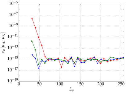
Results of numerical calculations involving a variety of numerical parameters with the complex analytic approach are provided in Fig.1. We find that while linear SCCT may be carried out with excellent accuracy the sequence of linear solutions entering the deformation problem is far more susceptible to instability. We ascribe this latter to the numerical division process involved in the calculation of ${}^{(m)}\tilde{\delta}/\omega^{|\beta|}$ where (small) local error in the vicinity of $\partial\Omega$ accumulates and is represented by spuriously populating high-order modes which in turn grow in scale with each iterate and gradually pollute low-order modes. Suppression of this is provided by filtering. While it is the case that either choice of $\beta=1$ or $\beta=-1/2$ in the ansatz on the potential $u$ appears to lead to convergence, unfortunately, as can be seen in Fig.1 (right) saturation in convergence still presents before numerical round-off.

Figure 1. Numerical complex-analytic approach applied to calculating scalar curvature deformation. Parameters selected according to $\mathcal{P}_{C}$ of Eq.(5.14) and $r_{\circ}=1.05$. The physical domain is selected with $\rho\in[1,\,2]$. Background metric coefficients $\left(\overline{F}(\rho(z)),\,\overline{G}(\rho(z)\right)$ are as in Eq.(5.10) with $M=1=P$ wherein we determine optimal radii parameters as $\langle r_{*}(F;\,n)\rangle_{n\leq n_{\sigma}}=3.3$ and $\langle r_{*}(G;\,n)\rangle_{n\leq n_{\sigma}}=1.2$ with $\sigma=10^{-10}$ (see Eq.(4.18)). (Left) Linear SCCT based on the seed potential $u_{1}$ defined in Eq.(5.11) where evaluation of Eq.(5.7) is based on refactoring involving the operators $D^{m}_{\rho}[\zeta,\,\eta,\,\theta][\cdot]$ and individual weight function terms which are calculated on an elliptic contour with $r_{\circ}$ as described in §5.1. Optimal radius of the potential function is given by $\langle r_{*}(u_{1};\,n)\rangle_{n\leq n_{\sigma}}=1.9$. Remaining parameter choices are denoted by: (red “$\blacklozenge$”): $\mathcal{P}_{C}(0)$; (blue “$\blacktriangleleft$”): $\mathcal{P}_{C}(1)$; (green “$\blacktriangleright$”): $\mathcal{P}_{C}(2)$. Even at moderate band-limit ($L_{\rho}\simeq 64$) we find that convergence to numerical round-off is attained. (Right) Absolute maximum of deformation over the real grid when the target ${}^{[3]}{\mathcal{R}}[g]$ is provided by Eq.(5.12) and Eq.(5.13) with number of iterations taken as $I=25$ (saturation in convergence verified by doubling). Deformation function $R_{i}(\rho(z))$ (Eq.(5.12)) optimal radii determined as $\langle r_{*}(R_{1};\,n)\rangle_{n\leq n_{\sigma}}=1.9$ and $\langle r_{*}(R_{2};\,n)\rangle_{n\leq n_{\sigma}}=6.4$. Denoted by: (red “$\blacklozenge$”): $R_{1}[\rho(z)]$ and $\mathcal{P}_{C}(0)$; (blue “$\blacktriangleleft$”): $R_{1}[\rho(z)]$ and $\mathcal{P}_{C}(1)$; (green “$\blacktriangleright$”): $R_{1}[\rho(z)]$ and $\mathcal{P}_{C}(2)$; (black “$\blacktriangledown$”): $R_{2}[\rho(z)]$ and $\mathcal{P}_{C}(0)$; (red “$\bullet$”): $R_{2}[\rho(z)]$ and $\mathcal{P}_{C}(1)$; (blue “$\blacksquare$”): $R_{2}[\rho(z)]$ and $\mathcal{P}_{C}(2)$. In order that the deformation sequence maintains stability we apply an Orszag-style low-pass filter via ${}^{(i)}u_{n}=0$ ($n>\frac{2}{3}L_{\rho}$) [49, 11]. Note: in both subfigures prior to saturation linear tails clearly indicate the property of exponential convergence.

As an alternative we pursue a hybrid scheme where terms involving $\partial_{\rho}^{n}[\omega]$ and $\partial_{\rho}^{n}[\mathcal{N}]$ that enter the factorisation of the integrand describing $A_{ij}$ in Eq.(5.7) are computed using arbitrary precision. All other quantities are calculated using standard, complex, floating-point arithmetic with the techniques of §4. An upshot of this approach is that for more generic weight functions such as:

$$C^{\infty}_{c}([-1,\,1])\ni\omega_{B}(\nu)=\begin{cases}\exp\left(1-[1-\nu^{2}]^{-1}\right),&\nu\in(-1,\,1);\\ 0,&\nu\notin(-1,\,1);\end{cases}$$ (5.15)

entering the deformation term $\delta$ no inconveniences due to complex analytic extensions or essential singularities arise.

We introduce further metric coefficient functions (cf. Eq.(5.10)):

$$\begin{aligned} (\overline{F}_{A}(\rho),\,\overline{G}_{A}(\rho)):=&\left(1+\sin^{2}(\pi\rho),\,\rho^{2}\right),&(\overline{F}_{B}(\rho),\,\overline{G}_{B}(\rho)):=&\left(1+\sin^{2}\left(\frac{\pi\rho}{3}\right),\,\rho^{2}\right);\end{aligned}$$ (5.16)

$$\begin{aligned} (\overline{F}_{C}(\rho),\,\overline{G}_{C}(\rho)):=&\left(2+\rho+2\cos^{2}(4\rho),\,1+\rho^{4}\exp(-\rho)\right);\end{aligned}$$

to which the metrics $\overline{g}_{A}$, $\overline{g}_{B}$ and $\overline{g}_{C}$ are associated. For convenience, set:

$$\mathcal{P}_{H}:j\mapsto\begin{cases}\left(\mathfrak{f},\,N,\,\beta\right)\mapsto\left(1.2,\,4,\,-1/2\right),&j=0;\\ \left(\mathfrak{f},\,N,\,\beta\right)\mapsto\left(1.2,\,2,\,-1\right),&j=1;\\ \left(\mathfrak{f},\,N,\,\beta\right)\mapsto\left(0.8,\,4,\,-1/2\right),&j=2;\\ \left(\mathfrak{f},\,N,\,\beta\right)\mapsto\left(0.4,\,4,\,-1/2\right),&j=3.\end{cases}$$ (5.17)

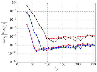
Results of numerical calculations making use of the hybrid scheme are shown in Fig.2 for various test deformation problems.

Figure 2. Numerical hybrid approach applied to calculating scalar curvature deformation. The maximum of the absolute value of the deformation on the real grid after $I=50$ iterations have been performed (saturation verified by doubling). In (red “$\blacklozenge$”): Target deformation $\delta$ constructed based on the seed potential $u_{1}$ of Eq.(5.11) and $\omega_{B}$ of Eq.(5.15) with background metric coefficients those of Eq.(5.10) where $(M,\,P)=(1,\,1)$ and $\rho_{\mathrm{min}}=1$ and $\rho_{\mathrm{max}}=2$. Parameters of $\hat{\omega}_{C}$ are selected via $\mathcal{P}_{H}$ of Eq.(5.17) where for this case $\mathcal{P}_{H}(0)$ is chosen. Now consider $\delta[{u}_{2}]$ constructed based on Eq.(5.11) with background metric $\overline{g}_{C}$ (see Eq.(5.16)). The physical domain is selected with $\rho\in[10,\,20]$. Remaining parameters chosen as: (blue “$\blacktriangleleft$”): $\mathcal{P}_{H}(0)$; (green “$\blacktriangleright$”): $\mathcal{P}_{H}(1)$. Now consider $\delta[\overline{g}_{B},\,R_{1},\,\hat{\omega}_{C}]$ constructed based on Eq.(5.12) and Eq.(5.13). Taking $\rho\in[5,\,10]$ where in: (black “$\blacktriangledown$”): $\mathcal{P}_{H}(0)$; (red “$\bullet$”): $\mathcal{P}_{H}(2)$. Finally consider $\delta[\overline{g}_{C},\,R_{2},\,\hat{\omega}_{C}]$ with $\rho\in[10,\,20]$ then in: (blue “$\blacksquare$”): $\mathcal{P}_{H}(1)$; (green “$\bigstar$”): $\mathcal{P}_{H}(3)$. Note: In all cases tested approximate exponential convergence is a clear feature.

As in Fig.1 we find that the results of calculations based on the hybrid approach presented in Fig.2 all lead to exponential convergence with a saturation in $\max_{j}\left|{}^{(I)}\delta(\rho_{j})\right|$ that is near numerical round-off. In contrast we find that no filtering is required and there does not appear to be much sensitivity with respect to how parameters of $\hat{\omega}_{C}$ are selected. Indeed, even with $\delta$ prepared such that $\omega_{B}$ is utilised we find convergence in the hybrid approach that does not degrade with increasing $L_{\rho}$. Due to these properties we henceforth shall only make use of this hybrid scheme and fix $\beta=-1/2$. We emphasise however that in the case of assembling $A_{ij}$ (see Eq.(5.7)) explicit refactoring of the integrand as described previously is required in order for numerical solutions to be found (linear or otherwise) based on both of the approaches investigated.

5.3. Axisymmetric deformation

Having investigated our numerical approach under the imposition of spherical symmetry in §5.1 we now turn our attention to scalar curvature deformation when the underlying metric is axisymmetric. It shall be assumed that this metric is of the form of Eq.(3.23) and that the coefficients appearing in Eq.(3.24) carry no $\varphi$ dependence. On account of the success of the mixed complex-analytic floating-point and arbitrary precision arithmetic hybrid approach a similar strategy shall be pursued here. As metric coefficients now carry a $\vartheta$ dependence that does not integrate out decompositions of fields shall be made by leveraging the SWSH functions and transformation algorithm described in §4.1.

Set $\Omega_{\rho}:=[\rho_{\mathrm{min}},\,\rho_{\mathrm{max}}]$, $\Omega_{\vartheta}:=[0,\,\pi]$ and $\Omega_{\varphi}:=\mathbb{S}^{1}$ then the full domain of interest is $\Omega_{\rho}\times\Omega_{\vartheta}\times\Omega_{\varphi}$; however, the $\varphi$ dependence is trivial and shall henceforth be suppressed. Taking the view that $\omega$ serves to impose boundary conditions by inducing decay towards $\partial\Omega_{\rho}$ on salient fields we shall continue to assume the dependence $\omega=\omega(\rho)$.

Thus, immediately we expand test and trial space functions respectively:

$${}_{0}\eta(\rho,\,\vartheta)= \sum_{m=0}^{L_{\rho}-1}\sum_{k=0}^{L_{\vartheta}}{}_{0}\eta_{mk}{}_{0}\Psi_{mk}(\rho,\,\vartheta), {}_{0}u(\rho,\,\vartheta)= \sum_{n=0}^{L_{\rho}-1}\sum_{l=0}^{L_{\vartheta}}{}_{0}u_{nl}{}_{0}\Phi_{nl}(\rho,\,\vartheta),$$ (5.18)

with expansion functions of both spaces treated symmetrically:

$${}_{0}\Psi_{nl}(\rho,\,\vartheta)={}_{0}\Phi_{nl}(\rho,\,\vartheta)=\Phi_{n}(\rho){}_{0}Y_{l}(\vartheta),$$ (5.19)

where $\Phi_{n}(\rho)$ is defined in Eq.(5.6) and ${}_{0}Y_{l}:={}_{0}Y_{l0}$ is an axisymmetric SWSH function as in §4.1. In the present context, the weak formulation of Eq.(2.7) becomes:

$$\sum_{n=0}^{L_{\rho}-1}\sum_{l=0}^{L_{\vartheta}}A_{mknl}\,{}_{0}u_{nl}=\tilde{\delta}_{mk},$$ (5.20)

where we have defined:

$$A_{mknl} :=\int_{\Omega}\left(L^{*}_{\overline{g}}\left[{}_{0}\Psi_{mk}(\rho,\,\vartheta)\right]\right)^{ij}\left(L^{*}_{\overline{g}}\left[{}_{0}\Phi_{nl}(\rho,\,\vartheta)\right]\right)_{ij}\omega(\rho)\mathchoice{{\hbox{$\displaystyle\sqrt{\overline{g}(\rho,\,\vartheta)\,}$}\lower 0.4pt\hbox{\vrule height=7.5pt,depth=-6.00003pt}}}{{\hbox{$\textstyle\sqrt{\overline{g}(\rho,\,\vartheta)\,}$}\lower 0.4pt\hbox{\vrule height=7.5pt,depth=-6.00003pt}}}{{\hbox{$\scriptstyle\sqrt{\overline{g}(\rho,\,\vartheta)\,}$}\lower 0.4pt\hbox{\vrule height=5.67776pt,depth=-4.54224pt}}}{{\hbox{$\scriptscriptstyle\sqrt{\overline{g}(\rho,\,\vartheta)\,}$}\lower 0.4pt\hbox{\vrule height=5.67776pt,depth=-4.54224pt}}}\,\mathrm{d}{\rho}\mathrm{d}{\vartheta},$$ (5.21)

$$\tilde{\delta}_{nl} :=\int_{\Omega}{}_{0}\Psi_{nl}(\rho,\,\vartheta)\tilde{\delta}(\rho,\,\vartheta)\omega(\rho)\mathchoice{{\hbox{$\displaystyle\sqrt{\overline{g}(\rho,\,\vartheta)\,}$}\lower 0.4pt\hbox{\vrule height=7.5pt,depth=-6.00003pt}}}{{\hbox{$\textstyle\sqrt{\overline{g}(\rho,\,\vartheta)\,}$}\lower 0.4pt\hbox{\vrule height=7.5pt,depth=-6.00003pt}}}{{\hbox{$\scriptstyle\sqrt{\overline{g}(\rho,\,\vartheta)\,}$}\lower 0.4pt\hbox{\vrule height=5.67776pt,depth=-4.54224pt}}}{{\hbox{$\scriptscriptstyle\sqrt{\overline{g}(\rho,\,\vartheta)\,}$}\lower 0.4pt\hbox{\vrule height=5.67776pt,depth=-4.54224pt}}}\,\mathrm{d}{\rho}\mathrm{d}{\vartheta};$$

and $\overline{g}(\rho,\,\vartheta)$ is the determinant of the background metric. To evaluate the internal contraction between $L_{\overline{g}}^{*}$ operators and implement a regularisation scheme analogous to that of §5.1 define the vector operator:

$$\boldsymbol{\mathcal{L}}[{}_{0}u]:=\left({}_{0}u,\,\partial_{\rho}\left[{}_{0}u\right],\,\partial_{\rho}^{2}\left[{}_{0}u\right],\,\overline{\eth}\left[\overline{\eth}\left[{}_{0}u\right]\right],\,\overline{\eth}\left[{}_{0}u\right],\,\partial_{\rho}\left[\overline{\eth}\left[{}_{0}u\right]\right],\,\eth\left[\overline{\eth}\left[{}_{0}u\right]\right]\right);$$ (5.22)

and introduce:

$$\mathcal{C}[{}_{0}\eta,\,{}_{0}u]=\sum_{q=1}^{7}\sum_{r=1}^{7}\boldsymbol{\mathcal{L}}[{}_{0}\eta]_{q}\,{}_{s}\mathcal{C}_{qr}\boldsymbol{\mathcal{L}}[{}_{0}u]_{r};$$ (5.23)

where the ($\omega$ independent) functions ${}_{s}\mathcal{C}_{qr}$ now complete specification of the contraction: they are the coefficients in front of all possible products of the derivatives of ${}_{0}u$. Each ${}_{s}\mathcal{C}_{qr}$ carries a spin-weight $s$ such that when combined with both $\boldsymbol{\mathcal{L}}[\cdot]$ the product has resultant spin-weight $0$.

The aforementioned factoring serves an additional purpose beyond numerical regularisation in the assembly of $A_{mknl}$. As the expansions of Eq.(5.18) are truncated such that for $m$ and $n$ together there is a storage requirement of $L_{\rho}^{2}$ elements, each of which in turn requires $k$ and $l$ to be specified, the number of elements appearing in $A_{mknl}$ (ignoring symmetry) scales as $\mathcal{O}(L_{\rho}^{2}(L_{\vartheta}+1)^{2})$. Thus, if all elements are immediately constructed and sampled then naive intermediate calculations involving $A_{mknl}$ result in a storage requirement scaling as $\mathcal{O}\left(2L_{\rho}^{2}(2L_{\rho}+2)(L_{\vartheta}+1)^{2})(L_{\vartheta}+2)\right)\sim\mathcal{O}(L_{\rho}^{3}L_{\vartheta}^{3})$.

Embedding a quadrature evaluation at the intermediate stage is more efficient. To accomplish this we perform a further regrouping of individual terms in the integrand of $A_{mknl}$. On account of the tensor product basis utilised the action of the weighted operator $\tilde{\boldsymbol{\mathcal{L}}}[\cdot]:=\omega(\rho)^{1/2}\boldsymbol{\mathcal{L}}[\cdot]$ may be decoupled to $\rho$ and $\vartheta$ specific subspaces where with Eq.(5.6) and Eq.(5.19):

$$\tilde{\boldsymbol{\mathcal{L}}}\left[{}_{0}\Phi_{nl}\right]=\sum_{q=1}^{7}\boldsymbol{\mathcal{L}}_{\rho}[\Phi_{n}]_{q}\boldsymbol{\mathcal{L}}_{\vartheta}[{}_{0}Y_{l}]_{q};$$ (5.24)

and the individual components of $\mathcal{\boldsymbol{\mathcal{L}}}_{\rho}[\Phi_{n}]_{q}$ are of the form of $D^{m}_{\rho}\left[\frac{1}{2},\,0,\,0\right][\Phi_{n}]$ (see Eq.(5.8)). Set:

$${}_{s}\tilde{\mathcal{C}}_{qr}(\rho,\,\vartheta):=\mathchoice{{\hbox{$\displaystyle\sqrt{\overline{g}(\rho,\,\vartheta)\,}$}\lower 0.4pt\hbox{\vrule height=7.5pt,depth=-6.00003pt}}}{{\hbox{$\textstyle\sqrt{\overline{g}(\rho,\,\vartheta)\,}$}\lower 0.4pt\hbox{\vrule height=7.5pt,depth=-6.00003pt}}}{{\hbox{$\scriptstyle\sqrt{\overline{g}(\rho,\,\vartheta)\,}$}\lower 0.4pt\hbox{\vrule height=5.67776pt,depth=-4.54224pt}}}{{\hbox{$\scriptscriptstyle\sqrt{\overline{g}(\rho,\,\vartheta)\,}$}\lower 0.4pt\hbox{\vrule height=5.67776pt,depth=-4.54224pt}}}{}_{s}\mathcal{C}_{qr}(\rho,\,\vartheta)\csc{\vartheta}={}_{0}\overline{N}(\rho,\,\vartheta)\mathchoice{{\hbox{$\displaystyle\sqrt{{}_{0}\overline{\gamma}(\rho,\,\vartheta)^{2}-{}_{-2}\overline{\gamma}(\rho,\,\vartheta){}_{+2}\overline{\gamma}(\rho,\,\vartheta)\,}$}\lower 0.4pt\hbox{\vrule height=9.30444pt,depth=-7.44359pt}}}{{\hbox{$\textstyle\sqrt{{}_{0}\overline{\gamma}(\rho,\,\vartheta)^{2}-{}_{-2}\overline{\gamma}(\rho,\,\vartheta){}_{+2}\overline{\gamma}(\rho,\,\vartheta)\,}$}\lower 0.4pt\hbox{\vrule height=9.30444pt,depth=-7.44359pt}}}{{\hbox{$\scriptstyle\sqrt{{}_{0}\overline{\gamma}(\rho,\,\vartheta)^{2}-{}_{-2}\overline{\gamma}(\rho,\,\vartheta){}_{+2}\overline{\gamma}(\rho,\,\vartheta)\,}$}\lower 0.4pt\hbox{\vrule height=6.53888pt,depth=-5.23112pt}}}{{\hbox{$\scriptscriptstyle\sqrt{{}_{0}\overline{\gamma}(\rho,\,\vartheta)^{2}-{}_{-2}\overline{\gamma}(\rho,\,\vartheta){}_{+2}\overline{\gamma}(\rho,\,\vartheta)\,}$}\lower 0.4pt\hbox{\vrule height=5.67776pt,depth=-4.54224pt}}}{}_{s}\mathcal{C}_{qr}(\rho,\,\vartheta),$$ (5.25)

then $A_{mknl}$ of Eq.(5.21) becomes:

$$A_{mknl}=\sum_{q=1}^{7}\sum_{r=1}^{7}\int_{0}^{\pi}\underbrace{\left[\int_{\rho_{\mathrm{min}}}^{\rho_{\mathrm{max}}}\boldsymbol{\mathcal{L}}_{\rho}[{\Psi_{m}}]_{q}\,{}_{s}\mathcal{\tilde{C}}_{qr}\boldsymbol{\mathcal{L}}_{\rho}[{\Phi_{n}}]_{r}\,\mathrm{d}{\rho}\right]}_{=:{}_{s}A_{mn}(\vartheta)}\boldsymbol{\mathcal{L}}_{\vartheta}[{}_{0}Y_{k}]_{q}\boldsymbol{\mathcal{L}}_{\vartheta}[{}_{0}Y_{l}]_{r}\sin\vartheta\,\mathrm{d}{\vartheta}.$$ (5.26)

The inner quadrature ${}_{s}A_{mn}(\vartheta)$ is numerically evaluated with a Clenshaw-Curtis rule [81] whereupon expansion with the family $({}_{s}Y_{j}(\vartheta))_{j=0}^{L_{\vartheta}}$ allows for evaluation of the outer quadrature.

Linear SCCT requires evaluation of $\delta(\rho,\,\vartheta)=\tilde{\delta}(\rho,\,\vartheta)\omega(\rho)$ appearing in the integrand of $\tilde{\delta}_{nl}$ of Eq.(5.21) for a given choice of seed potential $u(\rho,\,\vartheta)=\mathcal{N}(\rho)\tilde{u}(\rho,\,\vartheta)\omega(\rho)^{-1/2}$. This we accomplish by expressing $\partial_{\rho}^{m}\left[\omega(\rho)L_{\overline{g}}^{*}[u(\rho,\,\vartheta)]\right]$ for $m=0,\,1,\,2$ via the (non-zero) spin-weighted terms $\partial_{\rho}^{m}\left[\omega(\rho)\mathfrak{l}_{\rho\rho}[u(\rho,\,\vartheta)]\right]$ and $\partial_{\rho}^{m}\left[\omega(\rho){}_{s}\mathfrak{l}[u(\rho,\,\vartheta)]\right]$ based on the decomposition technique described in §3.3. In accordance with Eq.(2.8), $\delta(\rho,\,\vartheta)$ is formed by application of the frame representation of $L_{\overline{g}}[\cdot]$. Finally, resultant terms are expanded and regrouped such that all $\omega$ containing terms are collected and represented solely via the weighted operators $D^{n}_{\rho}$ introduced in Eq.(5.8). This is possible due to the assumption of the univariate $\rho$ dependence of $\omega$.

To close this section, we provide an update rule for metric coefficient functions when represented in terms of the spin-weighted components $\left({}_{0}\overline{N},\,{}_{\pm 1}\overline{N},\,{}_{0}\overline{\gamma},\,{}_{\pm 2}\overline{\gamma}\right)$. On account of the underlying axisymmetry we may drop the distinction between $\pm|s|$. This is a consequence of the particular properties of the coordinate representation of the SWSH and the $\eth$ operators: in axisymmetry the representations of ${}_{\pm s}Y_{l0}$ are real and agree even though, abstractly, these quantities have different spin-weight and therefore lie in different spaces.

Given a sequence of potential function solutions ${}^{(k)}u_{nl}$ define the update functional:

$$\mathcal{U}[\overline{f},\,\mathfrak{l};\,i](\rho,\,\vartheta):=\overline{f}(\rho,\,\vartheta)+\omega(\rho)\mathfrak{l}\left[\sum_{j=0}^{i}{}^{(j)}u(\rho,\,\vartheta);\,{}_{0}\overline{N},\,{}_{-1}\overline{N},\,{}_{0}\overline{\gamma},\,{}_{-2}\overline{\gamma}\right],$$ (5.27)

where $\mathfrak{l}$ is a general component of $L^{*}_{\overline{g}}[\cdot]_{ij}$ in the frame formalism (conventions of Eq.(3.23)). We may now write:

$$\prescript{(i+1)}{s\hphantom{)}}{\gamma}(\rho,\,\vartheta)= \mathcal{U}[{}_{s}\overline{\gamma},\,{}_{s}\mathfrak{l};\,i](\rho,\,\vartheta), \prescript{(i+1)}{-1\hphantom{)}}{N}(\rho,\,\vartheta)= \mathcal{U}[{}_{-1}\overline{N},\,{}_{-1}\mathfrak{l};\,i](\rho,\,\vartheta).$$ (5.28)

In order to update ${}_{0}\overline{N}$ first compute:

$${}^{(i+1)}\mathfrak{g}_{\rho\rho}(\rho,\,\vartheta)=\mathcal{U}[\overline{\mathfrak{g}}_{\rho\rho},\,\mathfrak{l}_{\rho\rho};\,i](\rho,\,\vartheta),$$ (5.29)

together with:

$$\prescript{(i+1)}{0\hphantom{)}}{\tilde{\gamma}}(\rho,\,\vartheta)=\left(\prescript{(i+1)}{0\hphantom{)}}{\gamma}(\rho,\,\vartheta)^{2}-\bigl{|}\prescript{(i+1)}{-2\hphantom{)}}{\gamma}(\rho,\,\vartheta)\bigr{|}^{2}\right)^{-1}.$$ (5.30)

Finally, based on Eq.(3.22) and Eq.(3.24) set:

$$\prescript{(i+1)}{0\hphantom{)}}{N}(\rho,\,\vartheta)^{2}= {}^{(i+1)}\mathfrak{g}_{\rho\rho}(\rho,\,\vartheta)+2\prescript{(i+1)}{0\hphantom{)}}{\tilde{\gamma}}(\rho,\,\vartheta)$$ (5.31)

$$\times\left(\prescript{(i+1)}{-1\hphantom{)}}{N}(\rho,\,\vartheta)^{2}\prescript{(i+1)}{+2\hphantom{)}}{\gamma}(\rho,\,\vartheta)-\left|\prescript{(i+1)}{-1\hphantom{)}}{N}(\rho,\,\vartheta)\right|^{2}\prescript{(i+1)}{0\hphantom{)}}{\gamma}(\rho,\,\vartheta)\right),$$

whereupon the positive root is taken.

5.4. Axisymmetric deformation: Test problem

On account of the restriction $\omega:=\omega(\rho)$ convergence properties in the axisymmetric case are largely controlled by the resolution selected in $\rho$. Essentially, for a sufficiently large, fixed $L_{\vartheta}$ behaviour as in §5.2 was observed. Hence, for the sake of expediency we will only provide an illustrative test problem here.

Introduce the background metric:

$$\overline{g}=\frac{\rho}{25}F(\vartheta)\mathrm{d}{\rho}\otimes\mathrm{d}{\rho}+\frac{\rho^{2}}{100}\left[F(\vartheta)(\omega\otimes\overline{\omega}+\overline{\omega}\otimes\omega)+G(\vartheta)\omega\otimes\omega+\overline{G}(\vartheta)\overline{\omega}\otimes\overline{\omega}\right],$$ (5.32)

where:

$$F(\vartheta):=1+{}_{0}Y_{1}(\vartheta),\qquad G(\vartheta):={}_{2}Y_{2}(\vartheta).$$ (5.33)

We now represent $\overline{g}$ in terms of the spin-weighted components $\left({}_{0}\overline{N},\,{}_{-1}\overline{N},\,{}_{0}\overline{\gamma},\,{}_{-2}\overline{\gamma}\right)$. According to the decomposition of Eq.(3.23) and Eq.(3.24) we may immediately take ${}_{-1}\overline{N}=0$, and it follows that ${}_{0}\overline{N}(\rho,\,\vartheta)=\rho\mathchoice{{\hbox{$\displaystyle\sqrt{F(\vartheta)\,}$}\lower 0.4pt\hbox{\vrule height=7.5pt,depth=-6.00003pt}}}{{\hbox{$\textstyle\sqrt{F(\vartheta)\,}$}\lower 0.4pt\hbox{\vrule height=7.5pt,depth=-6.00003pt}}}{{\hbox{$\scriptstyle\sqrt{F(\vartheta)\,}$}\lower 0.4pt\hbox{\vrule height=5.25pt,depth=-4.20003pt}}}{{\hbox{$\scriptscriptstyle\sqrt{F(\vartheta)\,}$}\lower 0.4pt\hbox{\vrule height=3.75pt,depth=-3.00002pt}}}/5$. The intrinsic metric expression provided by Eq.(3.14) together with the maps of Eq.(3.15) yields:

$${}_{-2}\overline{\gamma}(\rho,\,\vartheta)= \frac{\rho^{2}}{50}{}_{-2}Y_{2}(\vartheta), {}_{0}\overline{\gamma}(\rho,\,\vartheta)= \frac{\rho^{2}}{100}\left(1+{}_{0}Y_{1}(\vartheta)\right).$$ (5.34)

The target scalar curvature shall be defined by:

$${\mathcal{R}}[g]:={\mathcal{R}}[\overline{g}]+\delta(\rho,\,\vartheta;\,\omega),$$ (5.35)

where in this section we take $\delta$ as:

$$\delta(\rho,\,\vartheta;\,\omega)= \frac{401}{47}\sin(4\rho){}_{0}Y_{4}(\vartheta)\omega(\rho).$$ (5.36)

Spin-weighted metric coefficients shall be sampled in $\Omega_{\rho}$ with mapped $\Gamma_{E}$ at fixed $r_{B}=1.6$ in order to numerically determine partial derivatives in $\rho$ based on the techniques discussed in §4.3 which are then sampled back to the real, mapped Chebyshev-Gauss-Lobatto grid (see [81] for a definition). Approximation in $\Omega_{\vartheta}$ is based on the axisymmetric SWSH algorithm discussed in §4.2.

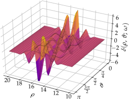
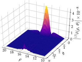
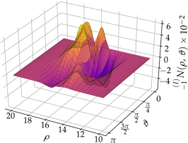
A representative calculation for local scalar-curvature deformation is inspected in Fig.3 where geometric quantities are updated as described at the end of §5.3.

Figure 3. Background scalar curvature ${\mathcal{R}}[\overline{g}]$ associated with spin-weighted metric coefficients of $\overline{g}$ as in the text. The deformation $\delta(\rho,\,\vartheta)$ of Eq.(5.36) used to generate the target ${\mathcal{R}}[g]$ defined by Eq.(5.35) and magnitude of updated deformation $\left|{}^{(I)}\delta(\rho,\,\vartheta)\right|$ where $I=80$ iterations have been taken (saturation verified by doubling) is also depicted. The weight function is $\hat{\omega}_{C}(\rho)$ of Eq.(5.2) with parameters provided via $\mathcal{P}_{H}(0)$ of Eq.(5.17); this enforces $\delta\rightarrow 0$ as $\rho\rightarrow\partial\Omega_{\rho}$. Band-limits are selected as $L_{\rho}=128$ and $L_{\vartheta}=64$. Note the comparable magnitudes of ${\mathcal{R}}[\overline{g}]$ and $\delta$. Colouring of all subfigures corresponds to function values.

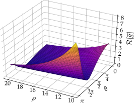
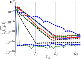
A further remark is in order: while we have selected $\overline{g}$ such that ${}_{-1}\overline{N}=0$ there is no reason a priori to inhibit non-zero updates to this quantity during the iterative construction of ${\mathcal{R}[g]}$. Indeed we find this is the case for the present example (see Fig.4 (left)). Furthermore, on account of $\left|{}^{(i)}\delta(\rho,\,\vartheta)\right|$ accumulating towards $\partial\Omega_{\vartheta}$ when $\rho\simeq\frac{1}{2}(\rho_{\mathrm{max}}-\rho_{\mathrm{min}})$ we inspect how modal representations in $\rho$ decay when averaging is performed over $\vartheta$ and vice versa for background and updated metric coefficients together with the spin-weighted contraction coefficients ${}_{s}\mathcal{C}_{mn}$ of Eq.(5.23). In order to compactly represent ${}_{s}\mathcal{C}_{mn}$ an additional average over $m$ and $n$ is taken over all coefficients of fixed $s$. Coefficient decay is displayed in Fig.4 (middle, right). It is clear that on average coefficients do not display any spurious growth – this was also verified by inspecting individual ${}_{s}\mathcal{C}_{mn}$.

Figure 4. (Left) Resulting ${}^{(I)}_{-1}N(\rho,\,\vartheta)$ where $I=80$ for scalar curvature deformation with $\overline{g}$ and target $\delta$ of the text. Color selected according to ${}^{(I)}_{-1}N(\rho,\,\vartheta)$ value. (Middle) Normalised (by maximum absolute value) modal representations of functions with RMS over nodal $\vartheta$ samples where the function ${}_{s}f$ in (green “$\blacktriangleright$”, blue “$\blacktriangleleft$”, red “$\blacklozenge$”): ${}_{-2}\mathcal{C}_{mn}$, ${}_{-1}\mathcal{C}_{mn}$ and ${}_{0}\mathcal{C}_{mn}$ are selected respectively; (black solid, dashed “$\blacktriangledown$”): ${}_{0}\overline{N}$ and ${}^{(I)}_{\;\,0}{\overline{N}}$ respectively; (red “$\bullet$”): ${}^{\;(I)}_{-1}{N}$; (green solid, dashed “$\bigstar$”): ${}_{-2}\overline{\gamma}$ and ${}^{\;(I)}_{-2}{\gamma}$ respectively; (blue solid, dashed “$\blacksquare$”): ${}_{0}\overline{\gamma}$ and ${}^{(I)}_{\;\,0}{\gamma}$ respectively. (Right) Legend as before; normalised, RMS is now performed over nodal $\rho$ samples. Note: While construction of the Picard iteration damps the original exponential decay we find that coefficient magnitudes are sufficiently small at larger band-limits to accurately represent functions.

5.5. Gluing: Internal binary black holes and external Schwarzschild

We finally turn our attention to a problem of physical interest, namely the gluing of binary black hole (Brill-Lindquist [13] and Misner [65]) data to an exterior asymptotic Schwarzschild end. As in [28] our approach shall be construction of initial data on a spherical shell $\Omega=\Omega_{\rho}\times\Omega_{\vartheta}\times\Omega_{\varphi}$. On the interior ball bounded by $\Omega$ for which $\rho<\rho_{\mathrm{min}}$ a vacuum constraint (at a MIT symmetry) satisfying, asymptotically Euclidean metric $g_{E}$ is prescribed whereas to the exterior of $\Omega$ where $\rho>\rho_{\mathrm{max}}$ Schwarzschild initial data are chosen. For $g_{\Omega}$ where $\rho\in\Omega_{\rho}$ we select a suitably truncated combination of these choices (see Eq.(5.41)). In contrast to [28] our numerical scheme does not follow the proposal of [41]. We rather attempt to follow the construction of Corvino’s proof [24] as closely as possible.

For convenience, recall the Euclidean metric with $\dim(\Sigma)=3$ in spherical coordinates:

$$\delta_{\mathrm{Euc}}=\mathrm{d}{\rho}\otimes\mathrm{d}{\rho}+\rho^{2}\left(\mathrm{d}{\vartheta}\otimes\mathrm{d}{\vartheta}+\sin^{2}\vartheta\,\mathrm{d}{\varphi}\otimes\mathrm{d}{\varphi}\right).$$ (5.37)

We can use conformal transformations so as to provide an interesting $g_{E}$ by rescaling $\delta_{\mathrm{Euc}}$ via the factor (function) $\psi$ as [6, 1]:

$$g_{E}=\psi^{4}\delta_{\mathrm{Euc}}.$$ (5.38)

Selection of initial data that can be interpreted as corresponding to a quantity of $\Xi$ black holes is provided by the Brill-Lindquist (BL) choice [13, 6]:

$$\psi =1+\sum_{\xi=1}^{\Xi}\frac{m_{\xi}}{2r_{\xi}}, r_{\xi} =|x^{i}-C^{i}_{\xi}|;$$ (5.39)

where $r_{\xi}$ is the (coordinate) separation from the centre $C^{i}_{\xi}$ of the $\xi^{\mathrm{th}}$ black hole. In order to compare with [28] we work within the context of axisymmetry where symmetrically spaced, on-axis, equal mass, binary black hole data, i.e., $\Xi=2$, $m=m_{1}=m_{2}$ and (in Cartesian coordinates) $C_{1}^{i}=(0,\,0,\,d/2)=-C_{2}^{i}$ is chosen.

Free parameters appearing in $g_{E}$ are fixed as $m=2$ and $d=10$ so as to facilitate comparison with [28]. A further reason for this selection is to have a scenario where the two interior black hole horizons do not intersect and to avoid the formation of a tertiary outer horizon which is the case if the inequality $m/d\lesssim 0.64$ is satisfied (see also [13]).

External to $\Omega$ we follow [24] and select Schwarzschild initial data in isotropic form [6]:

$$g_{S}=\left(1+\frac{M_{\mathrm{ADM}}}{2r}\right)^{4}\delta_{\mathrm{Euc}},$$ (5.40)

where $M_{\mathrm{ADM}}$ is the mass of the full $g$ on $\Sigma$ which is to satisfy ${\mathcal{R}}[g]=0$. The underlying axisymmetry together with invariance under $z\rightarrow-z$ for $g_{E}$ entails that $g_{S}$ need not be shifted from the origin and the only physical parameter to be adjusted for the gluing construction is $M_{\mathrm{ADM}}$.

On $\Omega$ put:

$$\overline{g}_{\Omega}=\chi_{R}g_{E}+(1-\chi_{R})g_{S},$$ (5.41)

where $\chi_{R}$ is the mapped cut-off function described at the start of §5. The $\omega$ entering the metric coefficient update formulae together with the weak formulation of Eq.(5.21) is selected as $\hat{\omega}_{C}$ of Eq.(5.2) with $\mathfrak{f}=6/5$ and in both $\chi_{R}$ and $\hat{\omega}_{C}$ polynomial decay with $N=4$ is chosen.

In the present context a further complication resulting from constant (i.e. zero) ${\mathcal{R}}$ exists. Specifically, if $g\rightarrow\delta_{\mathrm{Euc}}$ then as explained in §2.2 the kernel of the formal adjoint $L_{g}^{*}[\cdot]_{ij}$ becomes non-trivial and a modified, projected problem must instead be treated. In order to avoid extensive changes to our numerical scheme we propose to solve Eq.(5.20) via truncated singular-value decomposition (TSVD) [79]. For a more general choice of axisymmetric $g_{E}$ (no longer invariant under $z\rightarrow-z$) the centre of $g_{S}$ may also need adjustment during the gluing process thus we have two degrees of freedom if we view $g_{S}$ as a parameterised family of candidate solutions – accordingly all but the two smallest singular values $\sigma_{i}$ shall be retained.

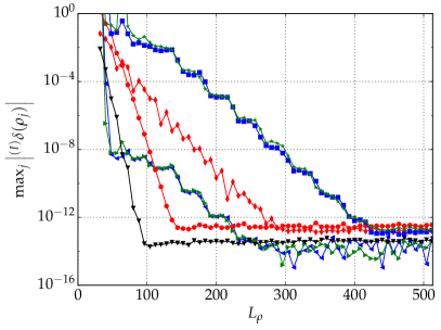
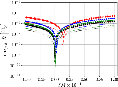
In Fig.5 we display the results of a numerical calculation where the gluing constructed is implemented as previously described. In addition to determination of all updated geometric quantities we must further fix the “optimal” $M_{\mathrm{ADM}}$ in the sense that the resulting scalar curvature is minimised (and ideally $0$). This is accomplished by varying about $2m$.

Figure 5. Maximum absolute value of scalar curvature after deformation for gluing of BL data. The domain $\Omega_{\rho}$ and $M_{\mathrm{ADM}}$ of $g_{S}$ is varied $M_{\mathrm{ADM}}\rightarrow 2m+\delta M$ where the background $\overline{g}_{\Omega}$ is that of Eq.(5.41). In both subfigures the number of iterations taken is $I=20$ (saturation verified by doubling) where solid lines correspond to $(L_{\rho},\,L_{\vartheta})=(128,\,32)$ and dotted lines to $(L_{\rho},\,L_{\vartheta})=(64,\,16)$. For $(L_{\rho},\,L_{\vartheta})=(128,\,32)$ with $\delta M$ selected such that the resulting scalar curvature is minimised put $\overline{r}:=\max_{\rho,\,\vartheta}\left|{\mathcal{R}}[\overline{g}_{\Omega}]\right|$. (Left) Internal value $\rho_{\mathrm{min}}$ fixed at $25$. Set $\Omega_{\rho}=\Omega_{\rho}(\mu):=[25,\,30+15\mu]$. Denoted in (red “$\blacklozenge$”): $\Omega_{\rho}(1)$, $\overline{r}=7.6\times 10^{-5}$; (blue “$\blacktriangleleft$”): $\Omega_{\rho}(2)$, $\overline{r}=1.5\times 10^{-5}$; (green “$\blacktriangleright$”): $\Omega_{\rho}(3)$, $\overline{r}=4.9\times 10^{-6}$; (black “$\blacktriangledown$”): $\Omega_{\rho}(4)$, $\overline{r}=2.0\times 10^{-6}$. (Right) Scaling applied to both end-points in the radial extent of $\Omega$. Set $\Omega_{\rho}=\Omega_{\rho}(\mu):=2^{\mu-1}[25,\,50]$. Denoted in (red “$\blacklozenge$”): $\Omega_{\rho}(0)$, $\overline{r}=4.1\times 10^{-5}$; (blue “$\blacktriangleleft$”): $\Omega_{\rho}(1)$, $\overline{r}=1.5\times 10^{-6}$; (green “$\blacktriangleright$”): $\Omega_{\rho}(2)$, $\overline{r}=4.8\times 10^{-8}$; (black “$\blacktriangledown$”): $\Omega_{\rho}(3)$, $\overline{r}=1.6\times 10^{-9}$. In both subfigures it is clear that $2m$ is approached from above with $M_{\mathrm{ADM}}\rightarrow 2m$ as $\Omega_{\rho}$ is enlarged. Furthermore, increasing band-limit does not significantly alter the value of $\delta M$ that minimises the resultant scalar curvature.

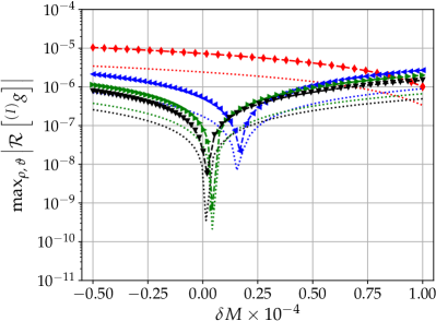
In agreement with [28] we find that the mass parameter entering $g_{S}$ must satisfy $M_{\mathrm{ADM}}\geq 2m$ for the gluing construction to proceed. Qualitatively, similar behaviour is found when parameters selected for $\hat{\omega}_{C}$ and $\chi_{R}$ are modified.

In consideration of an MIT symmetry an alternative option for $g_{E}$ is possible. By making use of Eq.(5.38) and Eq.(5.39) with $\Xi=2$ in construction of $g_{E}$ we implicitly assumed a three-sheeted topology, i.e., black hole throats are disconnected and not isometric [6]. Instead, one may work with Misner data [65], which, based on the technique of spherical inversion images allows for a symmetric identification of the throats resulting in a “wormhole” within what is now a single, asymptotically flat, multiply connected manifold. For an observer external to a horizon the consequence of this topological manipulation is a modification to the interaction energy [39, 40] and hence we investigate this within the context of the gluing construction.

For concreteness, in cylindrical coordinates $(r,\varphi,z)$ the Euclidean metric takes the form:

$$\delta_{\mathrm{Euc}}=\mathrm{d}{r}\otimes\mathrm{d}{r}+r^{2}\mathrm{d}{\varphi}\otimes\mathrm{d}{\varphi}+\mathrm{d}{z}\otimes\mathrm{d}{z}.$$ (5.42)

Misner data representing two equal-mass black holes aligned with $z$ and symmetrically situated about the origin is provided by [65, 6]:

$$\psi_{M}=1+\sum_{n=1}^{\infty}\frac{1}{\sinh(n\mu)}\left(\frac{1}{\mathchoice{{\hbox{$\displaystyle\sqrt{r^{2}+(z+z_{n})^{2}\,}$}\lower 0.4pt\hbox{\vrule height=9.30444pt,depth=-7.44359pt}}}{{\hbox{$\textstyle\sqrt{r^{2}+(z+z_{n})^{2}\,}$}\lower 0.4pt\hbox{\vrule height=9.30444pt,depth=-7.44359pt}}}{{\hbox{$\scriptstyle\sqrt{r^{2}+(z+z_{n})^{2}\,}$}\lower 0.4pt\hbox{\vrule height=6.53888pt,depth=-5.23112pt}}}{{\hbox{$\scriptscriptstyle\sqrt{r^{2}+(z+z_{n})^{2}\,}$}\lower 0.4pt\hbox{\vrule height=5.03888pt,depth=-4.03113pt}}}}+\frac{1}{\mathchoice{{\hbox{$\displaystyle\sqrt{r^{2}+(z-z_{n})^{2}\,}$}\lower 0.4pt\hbox{\vrule height=9.30444pt,depth=-7.44359pt}}}{{\hbox{$\textstyle\sqrt{r^{2}+(z-z_{n})^{2}\,}$}\lower 0.4pt\hbox{\vrule height=9.30444pt,depth=-7.44359pt}}}{{\hbox{$\scriptstyle\sqrt{r^{2}+(z-z_{n})^{2}\,}$}\lower 0.4pt\hbox{\vrule height=6.53888pt,depth=-5.23112pt}}}{{\hbox{$\scriptscriptstyle\sqrt{r^{2}+(z-z_{n})^{2}\,}$}\lower 0.4pt\hbox{\vrule height=5.03888pt,depth=-4.03113pt}}}}\right),$$ (5.43)

where $z_{n}:=\coth(n\mu)$ and $\mu$ is a free parameter which may be identified with the total mass:

$$\mu_{\mathrm{ADM}}=4\sum_{n=1}^{\infty}\frac{1}{\sinh(n\mu)}.$$ (5.44)

In fact any representative in this family of data is completely characterised by selection of $\mu$ on account of the proper length $L$ of a geodesic loop through the wormhole being [6]:

$$L=2\left(1+2\mu\sum_{n=1}^{\infty}\frac{n}{\sinh(n\mu)}\right).$$ (5.45)

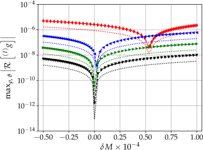
To provide a direct comparison with the previous setup we solve Eq.(5.44) for $\mu$ when $\mu_{\mathrm{ADM}}=4$ using standard numerical techniques to find $\mu=1.14960525757536$. This in turn fixes $\psi_{M}$ of Eq.(5.43) which, upon mapping to spherical coordinates allows us to take $g_{E}=\psi_{M}^{4}\delta_{\mathrm{Euc}}$. The results of this numerical calculation are shown in Fig.6.

Figure 6. Calculation of Fig.5 repeated with $g_{E}$ constructed based on Misner data (see text for details); all salient parameters as there unless otherwise stated. (Left) Internal value $\rho_{\mathrm{min}}$ fixed at $25$. Set $\Omega_{\rho}=\Omega_{\rho}(\mu)=[25,\,30+15\mu]$. Denoted in (red “$\blacklozenge$”): $\Omega_{\rho}(1)$, $\overline{r}=2.6\times 10^{-5}$; (blue “$\blacktriangleleft$”): $\Omega_{\rho}(2)$, $\overline{r}=5.2\times 10^{-6}$; (green “$\blacktriangleright$”): $\Omega_{\rho}(3)$, $\overline{r}=1.7\times 10^{-6}$; (black “$\blacktriangledown$”): $\Omega_{\rho}(4)$, $\overline{r}=6.8\times 10^{-7}$. (Right) Scaling applied to both end-points in the radial extent of $\Omega$. Set $\Omega_{\rho}=\Omega_{\rho}(\mu):=2^{\mu-1}[25,\,50]$. Denoted in (red “$\blacklozenge$”): $\Omega_{\rho}(0)$, $\overline{r}=1.4\times 10^{-5}$; (blue “$\blacktriangleleft$”): $\Omega_{\rho}(1)$, $\overline{r}=4.9\times 10^{-7}$; (green “$\blacktriangleright$”): $\Omega_{\rho}(2)$, $\overline{r}=1.6\times 10^{-8}$; (black “$\blacktriangledown$”): $\Omega_{\rho}(3)$, $\overline{r}=5.3\times 10^{-10}$. In both subfigures it is clear that $2m$ is again approached from above with $M_{\mathrm{ADM}}\rightarrow 2m$ as $\Omega_{\rho}$ is enlarged; efficiency is improved in contrast to Fig.5.

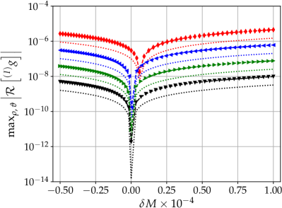
While it is the case that the new internal data reduces the required $\delta M$ and thus may be thought of as being more “efficient” we again find that the $M_{\mathrm{ADM}}$ parameterising the external Schwarzschild representative must be tuned to exceed the mass of $g_{E}$, that is, the metric on $\Omega$ tends to introduce additional energy to the gluing construction.

For both Brill-Lindquist and Misner data we numerically determined optimising masses (see Fig.5 and Fig.6 respectively) that allowed for gluing to exterior Schwarzschild to proceed at a variety of parameters. Recall that the kernel of $L_{\overline{g}_{\Omega}}^{*}[\cdot]_{ij}$ is only approximate and our TSVD procedure always discards the two smallest $\sigma_{i}$ associated with $A_{mknl}$ of Eq.(5.21) constructed based on $\overline{g}_{\Omega}$. It is thus important to inspect the full singular value spectrum of $A_{mknl}$ directly. Doing so (with values $\sigma_{i}$ ordered in descending magnitude) reveals distinct, discrete jumps in magnitude for the smallest two values however these are not particularly pronounced and as $\rho_{\mathrm{min}}$ or the extent of $[\rho_{\mathrm{min}},\,\rho_{\mathrm{max}}]$ is reduced a gradual decay is instead found. This is not unexpected for it is the case that ${\mathcal{R}}[\overline{g}_{\Omega}]\rightarrow 0$ only when $\rho\rightarrow\infty$, i.e., we are only working with an approximate kernel for $L_{\overline{g}_{\Omega}}^{*}[\cdot]_{ij}$. This may be responsible for the larger values of $\max_{\rho,\,\vartheta}\left|\mathcal{R}\left[{}^{(I)}g\right]\right|$ observed during use of smaller gluing regions. On account of this, a potential alternative approach to treat the kernel numerically may be to make use of the controlled filtering offered by a Tikhonov regularisation scheme [86, 69, 48], which we shall consider elsewhere.

6. Discussion and conclusion

In this work we have demonstrated a new numerical technique directly inspired by and based on the exterior asymptotic gluing (EAG) construction result of Corvino [24] that does not rely on a conformal Lichnerowicz-York decomposition of the constraints nor the Brill-wave ansatz approach of [41, 28, 74]. Our technique enabled fashioning of new solutions to the Einstein constraints in vacuum at a moment-in-time (MIT) symmetry based on a choice of internal Brill-Lindquist (BL) or Misner data glued over a transition region to a Schwarzschild exterior $g_{S}$. It appears that quite general asymptotically Euclidean, internal data may be glued in this sense. Unfortunately, for all calculations we performed, $M_{\mathrm{ADM}}$ of the interior set appeared as a lower bound in the sense that to construct composite initial data $(\Sigma,\,g)$ the parameter $M=M_{\mathrm{ADM}}+\delta M$ entering $g_{S}$ and enabling the gluing to proceed satisfied $\delta M\geq 0$. Thus a reduction of $M_{\mathrm{ADM}}$ based on BL internal data as claimed by [41] to be possible could not be found. This conclusion agrees with the general indications provided by the numerical results of [28, 74].

It would be of considerable interest to extend our numerical technique to incorporate a generalisation of Corvino’s result to EAG on Kerr as in [26]. For EAG on Kerr the proof technique remains similar albeit the MIT symmetry condition is relaxed. In particular, this means that the full constraint system must be considered inasmuch as the momentum constraint is no longer trivially satisfied due to the appearance of extrinsic curvature $K_{ij}$. From the point of view of numerical technique it should be feasible to employ a similar approach as in the EAG Schwarzschild scenario demonstrated here. However, clearly the system is considerably more involved. Potentially, while the technique of truncated singular value decomposition may still be feasible in treatment of the approximate kernel appearing in the adjoint linearisation of the full constraints a more geometric approach based on the Killing initial data interpretation (briefly described in §2.2) may be required.

An upshot of the increase in intricacy is a reduction in the rigidity of the possible composite $(\Sigma,\,g_{ij},\,K_{ij})$ forming initial data sets. For instance an analogous investigation to that made in this work could be based on internal Bowen-York initial data [10] and a similar question as to whether spurious gravitational wave content may be reduced could be asked. As we have not made use of conformal techniques (other than for the sake of convenience in specifying data to glue) this question is not obstructed by the results of [34, 59, 58] and may be worthwhile exploring further in this new setting.

Finally, composite data sets based on EAG would be of great interest to evolve numerically in order to better understand their dynamical properties. A potential path towards this end has been proposed in [28] where the property of an exact Schwarzschild exterior is exploited to allow for a hyperboloidal evolution scheme to proceed. We leave such investigations open to future work.

7. Appendix

Suppose $\overline{g}\neq\delta_{\mathrm{Euc}}$ then the $L_{\overline{g}}^{*}[\cdot]_{ij}$ of Eq.(2.5) can be seen to have trivial kernel provided that $\overline{\mathcal{R}}$ is non-constant with the following formal calculation based on [31, 24]. Assume $f\in\ker(L_{\overline{g}}^{*})$ then by contraction of Eq.(2.5):

$$0=\left(L_{\overline{g}}^{*}[f]\right)_{ij}\Longleftrightarrow \overline{\nabla}_{(i}\overline{\nabla}_{j)}f=\overline{\mathrm{Ric}}_{ij}f+\overline{g}_{ij}\overline{\nabla}^{2}[f],$$ (7.1)

$$\Longrightarrow \overline{\nabla}^{2}[f]=-\frac{1}{2}\overline{\mathcal{R}}f.$$

Whereas taking the divergence yields:

$$\overline{\nabla}{}^{j}[\overline{\nabla}{}_{i}[\overline{\nabla}{}_{j}[f]]] =\overline{\nabla}^{j}[\overline{\mathrm{Ric}}{}_{ij}]f+\overline{\mathrm{Ric}}{}_{ij}\overline{\nabla}^{j}[f]+\overline{\nabla}{}_{i}[\overline{\nabla}{}^{k}[\overline{\nabla}{}_{k}[f]]],$$ (7.2)

$$=\overline{g}^{kj}\left(\overline{R}{}_{kij}{}^{l}\overline{\nabla}_{l}[f]+\overline{\nabla}{}_{i}[\overline{\nabla}{}_{k}[\overline{\nabla}{}_{j}[f]]]\right)=\overline{\mathrm{Ric}}{}_{ij}\overline{\nabla}{}^{j}[f]+\overline{\nabla}{}_{i}[\overline{\nabla}{}^{k}[\overline{\nabla}{}_{k}[f]]],$$

$$\Longrightarrow 0 =\overline{\nabla}{}^{j}[\overline{\mathrm{Ric}}{}_{ij}]f.$$

To rewrite this in terms of the scalar curvature we make use of the Bianchi identity [84]:

$$\overline{\nabla}{}_{[i}\overline{R}{}_{jk]l}{}^{m}=0,$$ (7.3)

which once contracted yields:

$$\overline{\nabla}{}_{i}\left[\overline{R}{}_{jkl}{}^{i}\right]+\overline{\nabla}{}_{j}\left[\overline{\mathrm{Ric}}{}_{kl}\right]-\overline{\nabla}{}_{k}\left[\overline{\mathrm{Ric}}{}_{jl}\right]=0,$$ (7.4)

and once further:

$$\overline{\nabla}{}_{i}[\overline{\mathcal{R}}]=\frac{1}{2}\overline{\nabla}{}^{j}[\overline{\mathrm{Ric}}{}_{ij}].$$ (7.5)

Thus Eq.(7.2) and Eq.(7.5) show:

$$0=\overline{\nabla}{}_{i}[\overline{\mathcal{R}}]f.$$ (7.6)

That is, at points where $f$ does not vanish the gradient of $\overline{\mathcal{R}}$ must vanish. Consider now the behaviour of $f$ along an affinely parametrised geodesic $\gamma(s)$ with tangent vector $t^{i}$. Then directional derivatives $\overline{D}$ of $f$ along $\gamma$ are:

$$\overline{\mathrm{D}}_{s}\left[f(\gamma(s))\right] =f^{\prime}(s)=t^{i}\overline{\nabla}{}_{i}[f],$$ (7.7)

$$\overline{\mathrm{D}}^{2}_{s}\left[f(\gamma(s))\right] =f^{\prime\prime}(s)=t^{j}\overline{\nabla}{}_{j}[t^{i}\overline{\nabla}{}_{i}[f]]=\underbrace{t^{j}\left(\overline{\nabla}{}_{j}[t{}^{i}]\right)}_{=0}\overline{\nabla}{}_{i}[f]+t^{j}t^{i}\overline{\nabla}{}_{j}[\overline{\nabla}{}_{i}[f]];$$

where we made use of the geodesic equation [73]. With Eqs. 2.5 and 7.1 we find an ODE for the behaviour of $f$ along $\gamma$:

$$f^{\prime\prime}(s)=t^{i}t^{j}\left(\overline{\mathrm{Ric}}{}_{ij}-\frac{1}{2}\overline{g}_{ij}\overline{\mathcal{R}}\right)f(s).$$ (7.8)

Now when $f$ and $\overline{\nabla}{}_{i}[f]$ vanish at $x_{0}:=\gamma(0)$ then $f(\gamma(0))=0=f^{\prime}(\gamma(0))$ and hence by Eq.(7.8) $f(\gamma(s))=0$. It follows that $f$ must vanish in an entire neighbourhood of $x_{0}$. Due to the elliptic condition of Eq.(7.1) Aronszajn’s unique continuation theorem [2] implies that $f$ must vanish everywhere which would result in a trivial $\ker(L_{\overline{g}}^{*})$.

Suppose instead $f(x_{0})=0$ and $\overline{\nabla}_{i}[f](x_{0})\neq 0$. Then $x_{0}$ is a regular value and the zero-set of $f$ is an embedded submanifold $\mathscr{S}$ of co-dimension $1$, i.e., an embedded surface in $\Omega$ [60]. Finally, this implies that $\overline{\nabla}_{i}[\overline{\mathcal{R}}]=0$ on $\Omega\setminus\mathscr{S}$ and by continuity $\overline{\mathcal{R}}$ is constant on all $\Omega$.

Therefore when $\overline{\mathcal{R}}$ is not constant $\ker(L_{\overline{g}}^{*})$ is trivial and consequently $L_{\overline{g}}^{*}$ must be injective.

References

- [1] Alcubierre, M. Introduction to 3+1 Numerical Relativity. International Series of Monographs on Physics. OUP Oxford, 2012.
- [2] Aronszajn, N. A unique continuation theorem for solutions of elliptic partial differential equations or inequalities of second order. J. Math. Pures Appl. 36 (1957), 235–249.
- [3] Ashtekar, A., Berger, B., Isenberg, J., and MacCallum, M. General Relativity and Gravitation: A Centennial Perspective. Cambridge University Press, 2015.
- [4] Avila, G. A. Asymptotic staticity and tensor decompositions with fast decay conditions. PhD thesis, Universität Potsdam, 2011.
- [5] Bartnik, R., and Isenberg, J. The Constraint Equations. In The Einstein Equations and the Large Scale Behavior of Gravitational Fields. Birkhäuser, Basel, 2004, pp. 1–38.
- [6] Baumgarte, T. W., and Shapiro, S. Numerical Relativity: Solving Einstein’s Equations on the Computer. Cambridge University Press, 2010.
- [7] Beyer, F., Daszuta, B., and Frauendiener, J. A spectral method for half-integer spin fields based on spin-weighted spherical harmonics. Classical and Quantum Gravity 32, 17 (2015), 175013.
- [8] Beyer, F., Daszuta, B., Frauendiener, J., and Whale, B. Numerical evolutions of fields on the 2-sphere using a spectral method based on spin-weighted spherical harmonics. Classical and Quantum Gravity 31, 7 (2014), 075019.
- [9] Bornemann, F. Accuracy and Stability of Computing High-order Derivatives of Analytic Functions by Cauchy Integrals. Foundations of Computational Mathematics 11, 1 (Feb. 2011), 1–63.
- [10] Bowen, J. M., and York, Jr., J. W. Time-asymmetric initial data for black holes and black-hole collisions. Physical Review D 21, 8 (Apr. 1980), 2047–2056.
- [11] Boyd, J. P. Chebyshev and Fourier Spectral Methods, 2 ed. Dover Books on Mathematics. Dover Publications, 2013.
- [12] Brill, D. R. On the positive definite mass of the Bondi-Weber-Wheeler time-symmetric gravitational waves. Annals of Physics 7, 4 (Aug. 1959), 466–483.
- [13] Brill, D. R., and Lindquist, R. W. Interaction Energy in Geometrostatics. Physical Review 131, 1 (July 1963), 471–476.
- [14] Canuto, C., Hussaini, M., Quarteroni, A., and Zang, T. Spectral Methods: Fundamentals in Single Domains. Scientific Computation. Springer Berlin Heidelberg, 2007.
- [15] Carlotto, A., and Schoen, R. Localizing solutions of the Einstein constraint equations. Inventiones mathematicae 205, 3 (Sept. 2016), 559–615.
- [16] Chruściel, P., Galloway, G., and Pollack, D. Mathematical general relativity: A sampler. Bulletin of the American Mathematical Society 47, 4 (2010), 567–638.
- [17] Chruściel, P. T. Anti-gravity à la Carlotto-Schoen. Séminaire Bourbaki, Exposé 1120 (Nov. 2016).
- [18] Chruściel, P. T., Corvino, J., and Isenberg, J. Construction of N-Body Initial Data Sets in General Relativity. Communications in Mathematical Physics 304, 3 (June 2011), 637.
- [19] Chruściel, P. T., and Delay, E. Existence of non-trivial, vacuum, asymptotically simple spacetimes. Classical and Quantum Gravity 19, 9 (2002), L71.
- [20] Chruściel, P. T., Isenberg, J., and Pollack, D. Gluing Initial Data Sets for General Relativity. Physical Review Letters 93, 8 (Aug. 2004), 081101.
- [21] Chruściel, P. T., Isenberg, J., and Pollack, D. Initial Data Engineering. Communications in Mathematical Physics 257, 1 (May 2005), 29–42.
- [22] Cook, G. B. Initial Data for Numerical Relativity. Living Rev. Relativity 3 (2000).
- [23] Cooley, J. W., and Tukey, J. W. An algorithm for the machine calculation of complex Fourier series. Mathematics of Computation 19, 90 (1965), 297–301.
- [24] Corvino, J. Scalar Curvature Deformation and a Gluing Construction for the Einstein Constraint Equations. Communications in Mathematical Physics 214, 1 (2000), 137–189.
- [25] Corvino, J., and Pollack, D. Scalar Curvature and the Einstein Constraint Equations. arXiv:1102.5050 [gr-qc] (Feb. 2011). arXiv: 1102.5050.
- [26] Corvino, J., and Schoen, R. M. On the Asymptotics for the Vacuum Einstein Constraint Equations. J. Differential Geom. 73, 2 (06 2006), 185–217.
- [27] Daszuta, B. Numerical scalar curvature deformation and a gluing construction. PhD thesis, University of Otago, 2018.
- [28] Doulis, G., and Rinne, O. Numerical construction of initial data for Einstein’s equations with static extension to space-like infinity. Classical and Quantum Gravity 33, 7 (2016), 075014.
- [29] Dray, T. A unified treatment of Wigner D functions, spin-weighted spherical harmonics, and monopole harmonics. Journal of Mathematical Physics 27, 3 (Mar. 1986), 781–792.
- [30] Evans, L. Partial Differential Equations. Graduate studies in mathematics. American Mathematical Society, 1998.
- [31] Fischer, A. E., and Marsden, J. E. Deformations of the scalar curvature. Duke Mathematical Journal 42, 3 (1975), 519–547.
- [32] Fornberg, B. Algorithm 579: CPSC: Complex Power Series Coefficients [D4]. ACM Trans. Math. Softw. 7, 4 (Dec. 1981), 542–547.
- [33] Fornberg, B. Numerical Differentiation of Analytic Functions. ACM Trans. Math. Softw. 7, 4 (Dec. 1981), 512–526.
- [34] Garat, A., and Price, R. H. Nonexistence of conformally flat slices of the Kerr spacetime. Physical Review D 61, 12 (May 2000). arXiv: gr-qc/0002013.
- [35] Garfinkle, D., and Isenberg, J. Critical behavior in Ricci flow, 2003.
- [36] Gautschi, W. Numerical Analysis. SpringerLink : Bücher. Birkhäuser Boston, 2011.
- [37] Geroch, R. Energy Extraction. Annals of the New York Academy of Sciences 224, 1 (Dec. 1973), 108–117.
- [38] Gilbarg, D., and Trudinger, N. Elliptic Partial Differential Equations of Second Order. Classics in Mathematics. Springer Berlin Heidelberg, 2015.
- [39] Giulini, D. Interaction energies for three-dimensional wormholes. Classical and Quantum Gravity 7, 8 (1990), 1271.
- [40] Giulini, D. On the Construction of Time-Symmetric Black Hole Initial Data. In Black Holes: Theory and Observation, Lecture Notes in Physics. Springer, Berlin, Heidelberg, 1997, pp. 224–243.
- [41] Giulini, D., and Holzegel, G. Corvino’s construction using Brill waves. arXiv:gr-qc/0508070 (Aug. 2005). arXiv: gr-qc/0508070.
- [42] Goldberg, J. N., Macfarlane, A. J., Newman, E. T., Rohrlich, F., and Sudarshan, E. C. G. Spin-s Spherical Harmonics and . Journal of Mathematical Physics 8, 11 (Nov. 1967), 2155–2161.
- [43] Gómez, R., Lehner, L., Papadopoulos, P., and Winicour, J. The eth formalism in numerical relativity. Classical and Quantum Gravity 14, 4 (1997), 977.
- [44] Gourgoulhon, E. Construction of initial data for 3+1 numerical relativity. Journal of Physics: Conference Series 91, 1 (Nov. 2007), 012001.
- [45] Grandclément, P., and Novak, J. Spectral Methods for Numerical Relativity. Living Rev. Relativity 12 (2009).
- [46] Greene, R., and Krantz, S. Function Theory of One Complex Variable. Graduate studies in mathematics. American Mathematical Society, 2006.
- [47] Hamilton, R. S. Three-manifolds with positive Ricci curvature. Journal of Differential Geometry 17, 2 (1982), 255–306.
- [48] Hansen, P., Nagy, J., and O’Leary, D. Deblurring Images: Matrices, Spectra, and Filtering. Fundamentals of Algorithms. SIAM, Society for Industrial and Applied Mathematics, 2006.
- [49] Hesthaven, J., Gottlieb, S., and Gottlieb, D. Spectral Methods for Time-Dependent Problems. Cambridge Monographs on Applied and Computational Mathematics. Cambridge University Press, 2007.
- [50] Hohmann, A., and Deuflhard, P. Numerical Analysis in Modern Scientific Computing: An Introduction. Texts in Applied Mathematics. Springer New York, 2012.
- [51] Huisken, G., and Ilmanen, T. The Inverse Mean Curvature Flow and the Riemannian Penrose Inequality. Journal of Differential Geometry 59, 3 (Nov. 2001), 353–437.
- [52] Isenberg, J., Maxwell, D., and Pollack, D. A gluing construction for non-vacuum solutions of the Einstein-constraint equations. Advances in Theoretical and Mathematical Physics 9, 1 (Jan. 2005), 129–172.
- [53] Isenberg, J., Mazzeo, R., and Pollack, D. Gluing and Wormholes for the Einstein Constraint Equations. Communications in Mathematical Physics 231, 3 (Dec. 2002), 529–568.
- [54] Isenberg, J., Mazzeo, R., and Pollack, D. On the Topology of Vacuum Spacetimes. Annales Henri Poincaré 4, 2 (Mar. 2003), 369–383.
- [55] Jang, P. S., and Wald, R. M. The positive energy conjecture and the cosmic censor hypothesis. Journal of Mathematical Physics 18, 1 (Jan. 1977), 41–44.
- [56] Katznelson, Y. An Introduction to Harmonic Analysis, 3 ed. Cambridge University Press, 2004.
- [57] Knowles, I., and Wallace, R. A variational method for numerical differentiation. Numerische Mathematik 70, 1 (Mar. 1995), 91–110.
- [58] Kroon, J. A. V. Asymptotic expansions of the Cotton-York tensor on slices of stationary spacetimes. Classical and Quantum Gravity 21, 13 (2004), 3237.
- [59] Kroon, J. A. V. Nonexistence of Conformally Flat Slices in Kerr and Other Stationary Spacetimes. Physical Review Letters 92, 4 (Jan. 2004), 041101.
- [60] Lee, J. Introduction to Smooth Manifolds. Graduate Texts in Mathematics. Springer, 2003.
- [61] Lyness, J. N. Numerical Algorithms Based on the Theory of Complex Variable. In Proceedings of the 1967 22Nd National Conference (New York, NY, USA, 1967), ACM ’67, ACM, pp. 125–133.
- [62] Lyness, J. N., and Sande, G. Algorithm 413: ENTCAF and ENTCRE: Evaluation of Normalized Taylor Coefficients of an Analytic Function. Commun. ACM 14, 10 (Oct. 1971), 669–675.
- [63] Mason, J., and Handscomb, D. Chebyshev Polynomials. CRC Press, 2002.
- [64] Miel, G., and Mooney, R. On the condition number of Lagrangian numerical differentiation. Applied Mathematics and Computation 16, 3 (Apr. 1985), 241–252.
- [65] Misner, C. W. The method of images in geometrostatics. Annals of Physics 24 (Oct. 1963), 102–117.
- [66] Moncrief, V. Spacetime symmetries and linearization stability of the Einstein equations. I. Journal of Mathematical Physics 16, 3 (Mar. 1975), 493–498.
- [67] Morrey, C. Multiple Integrals in the Calculus of Variations. Classics in Mathematics. Springer Berlin Heidelberg, 2009.
- [68] Nestruev, J. Smooth Manifolds and Observables. Graduate Texts in Mathematics. Springer New York, 2013.
- [69] O’Leary, D. Near-Optimal Parameters for Tikhonov and Other Regularization Methods. SIAM Journal on Scientific Computing 23, 4 (Jan. 2001), 1161–1171.
- [70] Penrose, R. Naked Singularities. Annals of the New York Academy of Sciences 224, 1 (Dec. 1973), 125–134.
- [71] Penrose, R., and Rindler, W. Spinors and Space-Time: Volume 1, Two-Spinor Calculus and Relativistic Fields. Cambridge Monographs on Mathematical Physics. Cambridge University Press, 1987.
- [72] Pfeiffer, H. P. The initial value problem in numerical relativity. Journal of Hyperbolic Differential Equations 02, 02 (June 2005), 497–520.
- [73] Poisson, E. A Relativist’s Toolkit. Cambridge University Press, 2004.
- [74] Pook-Kolb, D., and Giulini, D. Numerical Approach for Corvino-Type Gluing of Brill-Lindquist Initial Data. arXiv:gr-qc/1809.00935 (Sept. 2018). arXiv:gr-qc/1809.00935.
- [75] Press, W. Numerical Recipes 3rd Edition: The Art of Scientific Computing. Cambridge University Press, 2007.
- [76] Rácz, I., and Winicour, J. On solving the constraints by integrating a strongly hyperbolic system. arXiv:1601.05386 [gr-qc] (Jan. 2016). arXiv: 1601.05386.
- [77] Rivlin, T. An Introduction to the Approximation of Functions. Dover Books on Mathematics Series. Dover Publications, 2003.
- [78] Rubinstein, J. H., and Sinclair, R. Visualizing Ricci Flow of Manifolds of Revolution. Experimental Mathematics 14, 3 (Jan. 2005), 285–298.
- [79] Shores, T. Applied Linear Algebra and Matrix Analysis. Undergraduate Texts in Mathematics. Springer New York, 2007.
- [80] Tichy, W. The initial value problem as it relates to numerical relativity. Reports on Progress in Physics 80, 2 (2017), 026901.
- [81] Trefethen, L. Spectral Methods in MATLAB. Software, Environments, and Tools. Society for Industrial and Applied Mathematics, 2000.
- [82] Trefethen, L. Approximation Theory and Approximation Practice. Other Titles in Applied Mathematics. Siam, 2013.
- [83] Trefethen, L., and Weideman, J. The Exponentially Convergent Trapezoidal Rule. SIAM Review 56, 3 (Jan. 2014), 385–458.
- [84] Wald, R. General Relativity. University of Chicago Press, 1984.
- [85] Wang, H., and Huybrechs, D. Fast and accurate computation of Chebyshev coefficients in the complex plane. IMA Journal of Numerical Analysis (2016).
- [86] Yagle, E., A. Regularized Matrix Computations. Department of EECS, The University of Michigan, Ann Arbor, MI 48109-2122 (2005), 1–7.